Transfer Entropy on Rank Vectors

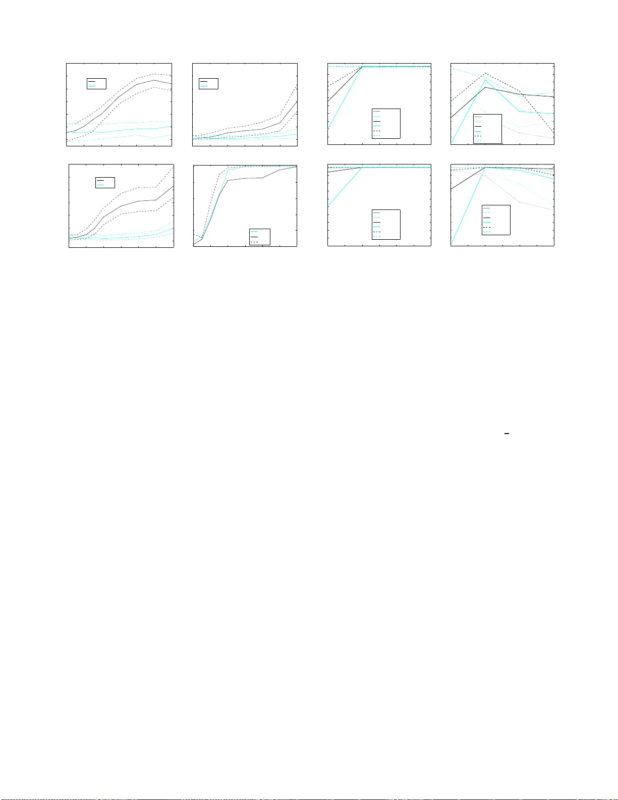
submitte d to Jour nal of Nonline ar Syst ems and Applic ations (Oct 2009) TRANSFER ENTR OPY ON RA NK VECTORS Dimitris Kugium tzis ∗ Abstract. T ransfer en trop y (TE) i s a p opular m easure of i nfor- mation flo w found to perform consisten tly w ell in different set tings. Sym boli c t ransfer en tropy (STE) is defined simi larly to TE but on the ranks of the componen ts of the reconstructed v ectors rather than the reconstructed v ectors themselves. First, w e corr ect STE b y f orming th e ranks for t he futu re sa mples o f th e response s ys- tem with regard to the curren t reconstructed v ector. W e give the grounds f or this mo dified v ersion of STE, which we call T ransfer En trop y on Rank V ectors (TER V). Then we prop ose to use more than one step ahead in the formation of the future of the resp onse in order to capture the inform ation flow from the driving system o v er a longer time hor i zon. T o assess the p erfor mance of STE, TE and TER V in detecting correctly the inf ormation flow w e use receiv er op erating cha racteristic (R OC) curv es form ed b y the mea- sure v alues in the tw o coupling dir ections computed on a n umber of realizations of known we akly coupled systems. W e also consider dif - ferent settings of state space r econstruction, time series length and observ ational noise. The results show that TER V indeed improv es STE and in some cases p erforms b etter than TE, particularly in the presence of noise, but ov erall TE gives more consisten t results. The use of multiple steps ahead i mprov es the accuracy of TE and TER V. Keywords. biv ari ate time series, coupling, causalit y , information measures, transf er en trop y , rank vec tors. 1 In tro duction The fundamental concept for the dep endence o f one v ari- able Y mea sured ov er time on ano ther v aria ble X mea- sured synchronously is the Granger c ausality [1]. While Granger defined the direction of interaction in terms of the co nt ribution of X in predicting Y , many v a riations of this concept hav e been developed, starting with linear approaches in the time and frequency domain (e.g. see [2, 3]) and ex tending to nonlinear a pproaches fo cusing on phase or even t synchronization [4 , 5, 6], comparing neigh- bo rho o ds of the reco nstructed p oints from the tw o time series [7, 8, 9, 10, 1 1, 12, 13], and measur ing the infor ma- tion flo w b etw ee n the time s eries [14, 15, 16, 1 7, 18]. Among the different prop osed measur es we c oncentrate here on the last clas s of measures, and particula r ly on the transfer entropy (TE) [14] and the most re cent v a riant of TE op er ating o n r ank vectors, called symbolic tra ns- ∗ D. Kugiumtzis is with the Departmen t of Mathematical, Ph ys- ical and Computational Sciences, F acult y of Engineering, A risto- tle Universit y of Thessaloniki, Thessaloniki 54124, Greece, e-mail: dkugiu@gen.auth.gr fer entrop y (STE) [1 7] (see also [19] for a simila r mea- sure). Ther e hav e b een a num b er of comparative studies on information flow measur es and other coupling mea- sures giving v ary ing re sults. In all the studies wher e TE was co nsidered, it p erformed a t leas t as go o d a s the other measures [20, 21, 22]. The STE measure is prop osed a s an improv emen t of TE in real world applications, where noise may mas k details of the fine structure, that can b e better treated by coarse discretization using ranks instead of sa mples . W e prop ose here a correction of STE. In the definition of TE the observ a ble of the resp onse at one time step ahead is a sca lar, but in STE it is taken as a rank vec- tor at this time index. W e modify STE to co nform with the definition of TE and give gro unds for the co r rectness of this mo dification. F urther, we allow for the future o f the res po nse to b e defined ov er mo re than o ne time steps. T o the b est of our knowledge this ha s not b een imple- men ted in TE, but it is the core element in the informa- tion flow mea sures of mea n c o nditional mutual info r ma- tion [18] and coarse-g rained transinforma tio n rate [15]. In many a pplica tions o n interacting flow systems, the sam- pling time may b e small and a sing le step ahead may no t regar d the time o f the resp o nse to the directed coupling, as in ele c tr o encephalogr aphy (EEG) [1 7, 23], and in the analysis of financial indices [1 6, 24]. The same may hold for maps: the transfer of information may b etter b e seen ov er more than one iteration of the interacting ma ps. W e compare TE, STE a nd o ur correc tio n of STE on mea- suring weak direc ted interaction in some k nown coupled systems a nd for different state spa ce reco nstructions, time series leng ths and also in the presence of no ise. W e also inv estiga te the change in the p erforma nce of these mea- sures when defining them for more than one step ahead. In the following, TE and STE mea sures ar e presented briefly in Section 2 , and the pr op osed mo dificatio n of TE is descr ibe d in Section 3. Then the r esults of the simu- lation s tudy compar ing the pr op osed measure to TE a nd STE are pre sented in Section 4, and discussed in Sec- tion 5. 2 Information flo w measures Let us supp os e that a r epresentativ e quan tit y of sys - tem X is measured giving a sca lar time series { x t } N t =1 and that w e have res pec tively { y t } N t =1 for Y , wher e X and Y po ssibly interact. Using the method of de- 1 2 Kugiumtzis D lays the r econstructed p oints from the tw o time se- ries are x t = [ x t , x t − τ x , . . . , x t − ( m x − 1) τ x ] a nd y t = [ y t , y t − τ y , . . . , y t − ( m y − 1) τ y ], allowing differen t delay pa- rameters τ x , τ y and embedding dimensions m x , m y for the s ystems X and Y , res pec tively . T ra nsfer entr opy (TE) is a measure of the information flow fro m the driving sys tem to the resp onse system. Spec ific a lly , TE estimates the entrop y in the resp onse system caused by its connection to the driving sy s tem, accounting for the entrop y generated internally in the r e - sp onse system [14]. TE for the causal effect of sys tem X on system Y can b e defined in terms o f the Shannon ent ropy H ( x ) = P p ( x ) log p ( x ) as TE X → Y = (1) − H ( y t +1 , x t , y t ) + H ( x t , y t ) + H ( y t +1 , y t ) − H ( y t ) , or directly in terms o f dis tribution functions as TE X → Y = X p ( y t +1 , x t , y t ) log p ( y t +1 | x t , y t ) p ( y t +1 | y t ) , (2) where p ( y t +1 , x t , y t ), p ( y t +1 | x t , y t ), and p ( y t +1 | y t ) a re the joint a nd co nditional proba bilit y mass functions (pmf ). The s ummation is ov er all the cells of a s uit- able par tition of the join t v a riable vectors a ppea ring as arguments in the pmfs o r entrop y terms. The estimation of TE req uires the estimation of the pmfs in eq.(2), o r the proba bilit y density functions as - suming the integral form and no binning . The pmfs are estimated dir ectly by the relative frequency of o cc ur rence of points in each ce ll, but finding a s uitable binning may be c hallenging [25, 26]. Moreov er, for high- dimens io nal reconstructio ns, the binning estimato rs are data demand- ing. Therefore estimators of the proba bilit y density func- tions are more appr opriate for TE estimation, suc h as kernels [27], nearest ne ig hbors [28], a nd c o rrelatio n sums [29]. W e follow the latter a pproach to estimate TE a nd recall first that without a ssuming discr etization e ach term of the form H ( x ) in (1) ex presses the differen tia l en- tropy of the vector v ariable x . The differential entropy can b e approximated from the corre la tion sum C ( x ) as H ( x ) ≃ ln C ( x ) + m ln r , wher e C ( x ) is the estimated cu- m ulative density o f inter-p oint distances at em bedding di- mension m and for a suitably small distance r [29]. Thus TE is estimated b y the cor relation sums as TE X → Y = lo g C ( y t +1 , x t , y t ) C ( y t ) C ( x t , y t ) C ( y t +1 , y t ) , (3) where C ( y t +1 , x t , y t ), C ( y t ), C ( x t , y t ) and C ( y t +1 , y t ) are the correla tio n sums for the po ints of the form [ y t +1 , x t , y t ], y t , [ x t , y t ] and [ y t +1 , y t ], re sp e ctively . The corres po nding v ector dimensio ns are 1 + m x + m y , m y , m x + m y and 1 + m y . T o acco un t for the differ e nt dimensions, we use the standar dized Euclidean norm for the dis tances. The so-ca lled symb olic tr ansfer entr opy (STE) is de- rived as the tr ansfer ent ropy defined on r ank vectors formed by the r econstructed p oints [17]. F or each p oint y t , the ranks of its comp onents in ascending order as- sign a rank vector ˆ y t = [ r 1 , r 2 , . . . , r m y ], where r j ∈ { 1 , 2 , . . . , m y } for j = 1 , . . . , m y , is the r a nk order of the comp onent y t − ( j − 1) τ y (for tw o equal co mp o nents of y t the smalle s t ra nk is as signed to the comp onent app ear ing first in y t ). Substituting also y t +1 in eq.(1) with the ra nk vector a t time t + 1, ˆ y t +1 , STE is defined as STE X → Y = (4) − H ( ˆ y t +1 , ˆ x t , ˆ y t ) + H ( ˆ x t , ˆ y t ) + H ( ˆ y t +1 , ˆ y t ) − H ( ˆ y t ) . The estimatio n of STE fro m eq.(4) is s traightforw ard as the pmfs a r e naturally defined on the rank vectors. There is a great adv antage o f using a rank vector ˆ y t ov er a bin- ning of y t , say using b bins for each comp onent: the pos- sible vectors from binning ar e b m y while the po ssible com- binations o f the rank vectors are m y !. F or exa mple, for b = m y = 4, there are 256 cells from binning and o nly 24 combinations of r ank vectors. Still, the estimation o f the probability of o ccur rence o f a rank vector b ecomes unsta- ble a s the dimension increases. Es pe cially , for the joint vector of ranks [ ˆ y t +1 , ˆ x t , ˆ y t ] the dimension is 2 m y + m x , for which the equiv a lent o f TE is [ y t +1 , x t , y t ] and ha s dimension 1 + m x + m y . 3 Mo dification of sym b olic trans- fer en trop y The conversion of the sca lar y t +1 to the rank vector ˆ y t +1 seems to hav e b een chosen in order to expres s y t +1 in terms o f rank s in [1 7]. Under this co n version, STE is not the direc t analo gue to TE using r anks instea d of s amples. The problem is no t so muc h the use of the s calar y t +1 or the vector y t +1 in the definition of TE in eq.(1) or eq.(2) b ecaus e for τ y = 1 p ( y t +1 , x t , y t ) = p ( y t +1 , x t , y t ), as all comp onents but y t +1 of the vector y t +1 are als o comp onents of y t . The same holds for the co nditional pmfs in eq .(2 ) and the tw o corr e lation sums in which y t +1 app ears in e q .(3). W e ela bo rate on the implication of the use of ˆ y t +1 below. Let us fir st assume that τ y = 1. A first problem lies in the fact that when deriving the ra nk vector ˆ y t +1 as- so ciated with y t +1 , the rank of the last comp onent of y t , y t − m y +1 , is not considere d. As an ex ample, co nsider the vector y t = [ y t , y t − 1 , y t − 2 , y t − 3 ] ′ with a co rresp ond- ing rank vector ˆ y t = [1 , 2 , 3 , 4 ], i.e. the sa mples decreas e with time. If the decrease contin ues a t the next time step then ˆ y t +1 = [1 , 2 , 3 , 4 ], if y t +1 is b et ween y t and y t − 1 then ˆ y t +1 = [2 , 1 , 3 , 4], if it is b etw ee n y t − 1 and y t − 2 then ˆ y t +1 = [3 , 1 , 2 , 4], a nd finally if y t +1 is lar g er than y t − 2 (the la rgest of all comp onents in y t +1 ) then ˆ y t +1 = [4 , 1 , 2 , 3]. The 4 p ossible scenario s are shown in Fig. 1. The definition of rank vector ˆ y t +1 accounts only for the p ossible rank p ositio ns of y t +1 with resp ect to the last m y − 1 samples, igno r ing the sample y t − m y +1 , her e T ra nsfer E ntrop y on Rank V ectors 3 y t t [1,2,3,4] t+1 t-1 t-2 t-3 y t+1 = ^ [2,1,3,4] y t+1 = ^ [3,1,2,4] y t+1 = ^ [4,1,2,3] y t+1 = ^ [4,1,2,3] y t+1 = ^ y t+1 ^ =1 y t+1 ^ =2 y t+1 ^ =3 y t+1 ^ =4 y t+1 ^ =5 y t+1 ^ Figure 1: Sketc h of a position of samples y t − 3 , y t − 2 , y t − 1 , y t and the p ossible rank p o s ition o f y t +1 together with the cor resp onding rank vector ˆ y t +1 defined for STE and the actua l ra nk of y t +1 considering all 5 samples. y t − 3 . With re gard to the same example, ˆ y t +1 = [4 , 1 , 2 , 3] assigns to b oth cases y t − 2 < y t +1 < y t − 3 and y t − 3 < y t +1 (see Fig. 1). In the e ntropy or proba bility terms of the definition of TE, y t +1 app ears together with y t , and there are 5 poss ible rank p ositions of y t +1 in the augment ed vec- tor [ y t +1 , y t , y t − 1 , y t − 2 , y t − 3 ], as s hown in Fig. 1. Thus for m y = 4 there are 5! = 1 20 different ra nk or der s for the joint vector [ y t +1 , y t ], but when for ming the join t rank vector [ ˆ y t +1 , ˆ y t ] (as in the computation of STE ) there are only 4! · (4! / 3 !) = 9 6 po s sible rank orde r s. In gen- eral, there ar e ( m y + 1)! p oss ible ra nk o rders for the joint vector [ y t +1 , y t ], but STE estimation repr e s ents them in m y ! · m y ! ( m y − 1)! rank orders of [ ˆ y t +1 , ˆ y t ]. The pmf o f the r ank vector derived fro m [ y t +1 , y t ] and the pmf of the r ank vector [ ˆ y t +1 , ˆ y t ] are shown in Fig. 2 for uniform white noise data a nd m y = 3. There are ( m y + 1)! = 24 e q uiprobable r ank or ders for [ y t +1 , y t ] (see Fig. 2a) but only m y ! · m y ! ( m y − 1)! = 18 different vectors [ ˆ y t +1 , ˆ y t ] are found, wher e m y ! = 6 of them have ab out double probabilit y , each corr esp onding to tw o distinct rank orders that could not b e distinguished (Fig. 2 b). This r esults in the under e stimation of the Shanno n en- 0 5 10 15 20 25 0 0.01 0.02 0.03 0.04 0.05 rank vector index i p(i) (a) 0 5 10 15 20 0 0.02 0.04 0.06 0.08 0.1 rank vector index i p(i) (b) Figure 2: (a) Estimated pmf for the r a nks of [ y t +1 , y t ] with m y = 3 (pro babilities ar e in ascending order ), where the samples y t are fro m a unifor m white noise time series of length N = 1 0 16 . (b) Same a s in (a) but for the ra nk vector [ ˆ y t +1 , ˆ y t ]. tropy . Using N = 10 16 samples and the ra nks of [ y t +1 , y t ] we found H = 4 . 5846 bits and using [ ˆ y t +1 , ˆ y t ] we found H = 4 . 0865 bits, while the true Shannon e n tropy is H = − log 2 (1 / 24) = 4 . 5850. Assuming a time s tep ahead T > 1, there are tw o scenarios to follow for the future s a mples of system Y : a single sample at time t + T , y t + T , o r all the sam- ples in the horizo n of length T , which we denote as y T t = [ y t +1 , . . . , y t + T ]. In the first ca se the po s sible rank orders of [ y t + T , y t ] are aga in ( m y + 1)! a nd for the seco nd case the p o ssible ra nk or ders of [ y T t , y t ] are ( m y + T )!. If instead we follow the for m in STE and s ubstitute ˆ y t + T to ˆ y t +1 , we hav e m y ! · m y ! ( m y − T )! po ssible rank s for [ ˆ y t + T , ˆ y t ], which regards neither of the tw o joint vector forms. F or example, for m y = 3 and T = 2, using the for m of STE [ ˆ y t + T , ˆ y t ] we ha ve 36 p ossible ra nk or ders, while for the joint vector form with a single sample T ahead, [ y t + T , y t ], the po ssible rank o rders are 24 and for all T s amples ahead, [ y T t , y t ], they are 120. F or uniform white noise data, the true entrop y for the ( m + 1)-dimensional aug- men ted vector is H = 4 . 5 850 and for ( m + T )-dimensional augmented vector is H = 6 . 90 69. Using the same esti- mation setup as b efore, we estimated correc tly these en- tropies a s H = 4 . 5847 a nd H = 6 . 9056 using the r ank orders o f [ y t + T , y t ] a nd [ y T t , y t ], resp ectively . Using the rank vector [ ˆ y t + T , ˆ y t ] we estimate H = 4 . 970 9 , which constitutes ov erestimation if co nsidering a single future sample at T time steps ahead and underestimation if con- sidering all the samples in the T time steps a head. F or the future resp onse at time T , we use the vector y T t of all the sa mples in the future ho rizon t + 1 , . . . , t + T . Thu s w e prop ose to substitute ˆ y t + T in STE of eq.(4) by ˆ y T t = [ ˆ y t +1 , . . . , ˆ y t + T ], the ranks o f y T t = [ y t +1 , . . . , y t + T ] in the augmented vector [ y T t , y t ]. The prop osed mea sure of trans fer entropy on rank vectors (TER V) for T steps ahead is TER V T X → Y = (5) − H ( ˆ y T t , ˆ x t , ˆ y t ) + H ( ˆ x t , ˆ y t ) + H ( ˆ y T t , ˆ y t ) − H ( ˆ y t ) . Since ˆ y T t app ears together with ˆ y t in the tw o entrop y terms in eq.(5), o ne ca n define [ ˆ y T t , ˆ y t ] as the r anks of the augmented vector [ y t + T , y t + T − 1 , . . . , y t +1 , y t ]. This is ac- tually equiv alent of taking the ranks of ˆ y t independently (as they app ear in the second and forth term in eq.(5)). The use of all the ranks for times t + 1 , . . . , t + T a ims at capturing the effect of X on the evolution of the time series of Y up to T time steps ahea d. Similar r easoning for T > 1 was used for other infor mation flow measur es [15, 18] and we hav e used T > 1 a lso for TE in [22]. The TER V mea sure is the direct analogue to TE using ranks and extends the measure o f infor mation flow from X to Y at time t for a range o f T time steps ahead t . The use of y T t instead o f y t + T increases the dimension of the joint space from m x + m y + 1 to m x + m y + T and can affect the stability of the estimation. Ho wev er , the results of a simulation study were in fav or of y T t against y t + T for bo th T E and TER V. Finally , we note that when a lag τ y > 1 is used for the state space reco ns truction of y t , there are up to m y ! · m y ! different rank vectors [ ˆ y t + T , ˆ y t ] in the co mputation 4 Kugiumtzis D of STE. On the other hand, for TER V there ar e ( T + m y )! different rank vectors [ ˆ y T t , ˆ y t ]. Thu s for τ y > 1, the distortion of the do ma in of the rank vectors b y STE may b e lar ge, e.g . for τ y = 2 a nd T = 1, the pmfs and ent ropies a re computed on ( m y + 1 )! different rank or ders for TE R V and m y ! · m y ! for STE. 4 Estimation of information mea- sures on sim ulated systems As it was s hown for the example of uniform white noise the dis tortion of the domain of the r ank vectors [ ˆ y T t , ˆ y t ] using the r a nk vectors [ ˆ y t + T , ˆ y t ] instead ha s a direct ef- fect on the estimation of e ntropy . While for uncoupled systems X and Y the entrop y terms involving [ ˆ y t + T , ˆ y t ] cancel out in the expr ession o f TER V (and resp ectively for STE), in the presenc e of co upling some bias is int ro- duced in the estimation of the co upling mea sure by STE. Using TE R V instead this bia s is removed. W e compare the estimation o f coupling (stre ngth and direction) with the mea sures TE, STE and TER V on sim- ulated systems. W e fir st standardize each time ser ies to hav e mean zero and standard deviation one, and this al- lows us to define a fixed radius for all systems in the computation o f TE , which we set r = 0 . 15. This choice is a trade-off of having enoug h p oints within a distance r to as sure stable es timation of the p oint distr ibutio n and maintaining s mall neighbor ho o ds to pr eserve details of the p o in t dis tribution. Still, for high- dimensional points, even this r adius may b e insufficient to provide stable es- timation. W e start with tw o unidirectionally coupled Henon maps [8] x t +1 = 1 . 4 − x 2 t + 0 . 3 x t − 1 y t +1 = 1 . 4 − cx t y t + (1 − c ) y 2 t + 0 . 3 y t − 1 with co upling strengths c =0,0.0 5,0.1,0.1 5,0.2,0 .3 ,0.4,0.5 and 0.6. The r esults on the coupling measur es TE, STE and TER V for T = 1, τ x = τ y = 1 and m x = m y = 2 are shown for 10 0 noise-free biv aria te time series of length N = 102 4 in Fig . 3. TE has the smallest v ariance and it seems to g ive the b est detection of the corre c t direction of coupling even for very weak coupling, whereas STE per forms worst. T o qua ntif y the level of discrimination of the corr ect direction of information flow, X → Y , often the net informa tio n flow is used, defined as the difference of the coupling mea sure in the tw o directions. Here, we assess the level of disc rimination in a statistical setting by computing the area under the r eceiver op era ting c harac- teristic (ROC) c urve on the 1 0 0 coupling measure v a lues for each direction, which we deno te A UR O C (e.g. see [30]). F or uncoupled systems, we ex p ect that AUR O C b e close to 0.5. F or a n info r mation flow measur e to detect coupling with grea t confidence A UR OC has to b e close to 1. In Fig. 3d, the AUR OC s hows that TE detects cou- pling with grea t confidence and obtains AUR O C=1 fo r 0 0.1 0.2 0.3 0.4 0.5 0.6 0 0.1 0.2 0.3 0.4 0.5 coupling TE (a) X−>Y Y−>X 0 0.1 0.2 0.3 0.4 0.5 0.6 0 0.01 0.02 0.03 0.04 0.05 0.06 coupling STE (b) X−>Y Y−>X 0 0.1 0.2 0.3 0.4 0.5 0.6 0 0.01 0.02 0.03 0.04 0.05 0.06 coupling TERV (c) X−>Y Y−>X 0 0.1 0.2 0.3 0.4 0.5 0.6 0.5 0.6 0.7 0.8 0.9 1 coupling AUROC (d) TE STE TERV Figure 3: (a) Median (so lid line) and 12 . 5 % and 87 . 5% per centiles (da s hed lines) of TE computed on 100 noise- free realiza tions o f length N = 1024 from the s ystem of tw o unidirectio nally coupled Heno n ma ps fo r v a rying coupling streng ths. The other parameter s a re T = 1, τ x = τ y = 1 and m x = m y = 2. The direction X → Y is shown with black lines and Y → X with grey (online cyan) lines, as shown in the legend. (b) Same as (a) but for STE. (c) Same as (a ) but for TER V. (d) AUR OC computed on the 100 rea lizations for each of the tw o di- rections and for the measures TE, STE and TE R V, as given in the legend. as low coupling strength as c = 0 . 1, follow ed by TE R V reaching the same level o f co nfidence at c = 0 . 15, while STE r eaches this level only a t stro ng co upling ( c = 0 . 5). The pe r formance of the coupling measur es changes in the presence o f no ise. F or the sa me setup as that in Fig. 3, but adding to the biv aria te time ser ie s 20% Gaus- sian white noise, w e obser ve that TER V per forms b est, follow ed by TE and having STE with the smalles t in- crease in the direction X → Y with the coupling strength (see Fig. 4). TER V has sma ller v ar iance than TE for small co upling strengths, which incre a ses its discriminat- ing power. Compar ing with the nois e-free case in Fig. 3 , TER V do es not seem to b e muc h affected by the addition of no ise, but TE do es not have the same robustness to noise. It is noted that using r = 0 . 15 was particular ly suitable to main tain some stability in TE o n the noisy data. The same s imu lations for r = 0 . 1 g av e much worse results [31]. The AUR OC curves in Fig. 3d ar e ordere d with TER V giving the hig hest and STE the low est AU- R OC for all coupling stre ng ths. W e have estimated TE, STE and TER V on the coupled Henon sys tem for different s ettings o f embedding dimen- sions, time steps a head T , time s eries length N and noise level. F or N s ma ll and m y large a nd mostly for no isy time s eries, the computation of TE was unstable due to the lack of p o ints within the given r adius. This expla ins T ra nsfer E ntrop y on Rank V ectors 5 0 0.1 0.2 0.3 0.4 0.5 0.6 0 0.1 0.2 0.3 0.4 0.5 coupling TE (a) X−>Y Y−>X 0 0.1 0.2 0.3 0.4 0.5 0.6 0 0.01 0.02 0.03 0.04 0.05 0.06 coupling STE (b) X−>Y Y−>X 0 0.1 0.2 0.3 0.4 0.5 0.6 0 0.01 0.02 0.03 0.04 0.05 0.06 coupling TERV (c) X−>Y Y−>X 0 0.1 0.2 0.3 0.4 0.5 0.6 0.5 0.6 0.7 0.8 0.9 1 coupling AUROC (d) TE STE TERV Figure 4: As Fig. 3, but with Gaussia n white noise with standard deviation 0.2 added to the standa rdized time series. that TE has s maller v ar iance for larger time serie s , a nd consequently b etter discr imina tion in the tw o directions of coupling . The measures do no t v ar y muc h with the embedding dimensio ns a nd STE shows the lar g est dep en- dency , es pe c ially when m x > m y . The b est re sults for all measures were o btained for m x = m y . In Fig. 5, the AUR OC is shown for the thre e mea- sures as a function of m y , where m x = m y , for very weak coupling ( c = 0 . 1), and for one and three s teps ahead, small and large time series and for nois e-free and no isy Henon data. It seems that estimating the informa tio n flow for T = 3 increases the detection of cor rect directio n of weak coupling for TE and TER V, but not for STE. F or the nois e-free data, the differences in AUR OC among the thr ee meas ures are small and all mea sures re a ch the highest level o f discriminatio n of the tw o dire c tions when m y > 2 . F o r m y = 2, A UR OC=1 is s till reached by TE and TER V but only with T = 3, w he r eas the AUR OC is m uc h smaller for STE r egardles s of T . This pattern is the s ame for b oth small and la rge N . F or nois y data, all measures p er form w orse and their A UR OC shows stro ng depe ndence on bo th m y and T . Similarly to the nois e - free case, the AUR OC is larger for T = 3 than fo r T = 1 for TE a nd TER V, but not for STE . The AUR O C of TE decreases with m y and for m y > 2 is lo w er than the A U- R OC for both STE and TER V. TER V obta ins the highest A UR OC v alues with T = 3 giving the overall b est results. The ab ov e res ults a re co nsistent for the tw o time series lengths shown in Fig. 5b a nd d with AUR O C v alues in- creasing from N = 1 024 to N = 4096 . Similar s imu lations have b een run for a R¨ ossler s ystem driving a Lor enz sy stem given a s (subsc r ipt 1 for R¨ ossler, 2 2.5 3 3.5 4 4.5 5 0.5 0.55 0.6 0.65 0.7 0.75 0.8 0.85 0.9 0.95 1 m y AUROC (a) TE T=1 TE T=3 STE T=1 STE T=3 TERV T=1 TERV T=3 2 2.5 3 3.5 4 4.5 5 0.5 0.55 0.6 0.65 0.7 0.75 0.8 0.85 0.9 0.95 1 m y AUROC (b) TE T=1 TE T=3 STE T=1 STE T=3 TERV T=1 TERV T=3 2 2.5 3 3.5 4 4.5 5 0.5 0.55 0.6 0.65 0.7 0.75 0.8 0.85 0.9 0.95 1 m y AUROC (c) TE T=1 TE T=3 STE T=1 STE T=3 TERV T=1 TERV T=3 2 2.5 3 3.5 4 4.5 5 0.5 0.55 0.6 0.65 0.7 0.75 0.8 0.85 0.9 0.95 1 m y AUROC (d) TE T=1 TE T=3 STE T=1 STE T=3 TERV T=1 TERV T=3 Figure 5: (a) AUR O C computed for different m y ( m x = m y ) on 100 realiza tions of the weakly coupled Henon sys- tem ( c = 0 . 1) for ea ch of the t w o directions, fo r the mea- sures TE, STE and TER V and for time steps ahead T , as g iven in the le g end. The time se r ies a re noise-free and N = 10 2 4. (b) As in (a) but fo r 20 % additive Ga ussian white no ise. (c) and (d) are as in (a) and (b) but for N = 4096. 2 for Lorenz) ˙ x 1 = − 6( y 1 + z 1 ) ˙ x 2 = 1 0( x 2 + y 2 ) ˙ y 1 = − 6( x 1 + 0 . 2 y 1 ) ˙ y 2 = 28 x 2 − y 2 − x 2 z 2 + cy 2 1 ˙ z 1 = − 6(0 . 2 + z 1 ( y 1 − 5 . 7)) ˙ z 2 = x 2 y 2 − 8 3 z 2 for coupling strengths c = 0 , 0 . 5 , 1 , 1 . 5 , 2 , 3 , 4 , 5 [32]. The observed v ar ia bles a re x 2 and y 2 and the sampling time is τ s = 0 . 1sec. Here, the res ults a re more v a rying than for the Henon system. First, there is strong er dependence of all mea sures, and particularly STE and TER V, on the t wo embedding dimensions. Again the bes t results are obtained for m x = m y , while fo r m x < m y the measure v alues in the cor rect direction X → Y ar e increased and for m x > m y the opp osite is observed leading to erroneous detection o f directio n of interaction. The effect of the dif- ferent formation of the rank future vector in STE and TER V can b e b etter s een for T > 1 and for small embed- ding dimensio ns . As shown in Fig. 6, for m x = m y = 3, while for T = 1 b oth rank measure s tend to give larg er v alues in the opp osite wrong direction Y → X , for T = 3 STE contin ues to give the same re sult but TER V p oints to the co rrect direction a t least for intermediate v alues of c . The ra nk meas ures s uffer fro m p ositive bias that in- creases with T and this is more obvious in TER V. When the tw o sy stems have different complexity the bias tends to be larger in the dir ection from the less complex (R¨ ossler) to the mo re complex (Lorenz) s ystem. F or T = 3 in Fig. 6b and d, the rank measur e v alues are larger for the direction X → Y when c = 0. This bias 6 Kugiumtzis D 0 1 2 3 4 5 −0.6 0 0.6 −0.6 0 0.6 −0.6 0 0.6 TERV STE TE coupling measure (a) X−>Y Y−>X 0 1 2 3 4 5 −0.6 0 0.6 −0.6 0 0.6 −0.6 0 0.6 TERV STE TE coupling measure (b) X−>Y Y−>X 0 1 2 3 4 5 −0.6 0 0.6 −0.6 0 0.6 −0.6 0 0.6 TERV STE TE coupling measure (c) X−>Y Y−>X 0 1 2 3 4 5 −0.6 0 0.6 −0.6 0 0.6 −0.6 0 0.6 TERV STE TE coupling measure (d) X−>Y Y−>X Figure 6: (a) Media n (solid line) a nd 12 . 5 % a nd 87 . 5 % per centiles (das he d lines) o f ea ch of the three cou- pling measure s computed on 10 0 nois e-free realizations of length N = 1024 from the R¨ ossle r–Lor e nz system for v arying coupling s tr engths. The o ther parameter s a re T = 1, τ x = τ y = 1 and m x = m y = 3. The direc- tion X → Y is shown with black lines and Y → X with grey (online cyan) lines, as shown in the legend, and the TE measure is at the top panel, STE in the middel, and TER V at the low pa nel. (b) As in (a) but for T = 3. (c) and (d) are a s in (a) and (b) but for 20% additive Gaussian white nois e. is present rega r dless of the coupling strength, so that the increase o f TE R V with the coupling strength still ca n b e observed. Ho wev er , AUR OC would not give useful re- sults as the discrimina tio n would be p er fect with TE R V for all c including c = 0. The p ositive bias of the r ank measures ca uses the lack of significa nce, i.e. obtaining po sitive v a lues in the absence of coupling, and this has serious implications in real world applications, where also the pr esence of interaction is in v estigated. The TER V mea sure has an a dv antage over TE in that it is more stable to noise. F o r the noise-free coupled R¨ ossler-Lor enz sys tem, TE detects clear ly the direction of coupling and its p erformance is enhanced when T in- creases from 1 to 3 . How ever, when noise is added to the data the estimation of TE is not stable and the large v ariance do es no t a llow to o bserve different levels o f TE in the t w o directio ns. The v ar iance is larger for T = 3 due to large r dimensio n of the state s pace vectors in the estimation o f the cor relation sums. W e hav e made the sa me s im ulations o n tw o weakly co u- pled Mac key-Glass systems given as d x d t = 0 . 2 x t − ∆ x 1 + x 10 t − ∆ x − 0 . 1 x t d y d t = 0 . 2 y t − ∆ y 1 + y 10 t − ∆ y + c 0 . 2 x t − ∆ x 1 + x 10 t − ∆ x − 0 . 1 y t , (6) where a gain the driving is from the first sy s tem X to the second system Y [33]. The tw o systems can hav e different complexity determined by the delay par ameters ∆ x and ∆ y . W e let ea ch ∆ para meter take the v alues 17, 30 , and 100 that, in the absence of coupling, regard systems of correla tion dimension at ab out 2 , 3 a nd 7, resp ectively [34]. Thus we hav e 9 different co upled Mackey-Glass sys- tems. All systems ar e solved using the function dd e23 of the computationa l e nvironment MA TL AB and are sam- pled at τ s = 4. The results are quite simila r to the r esults of the R¨ ossler-Lor enz system. Ther e is large v aria tio n of all measures, a nd pa rticularly the r ank measures, in the de- tection of direc tio n and streng th of coupling, dep ending on all tested facto rs: noise, embedding dimensions, fu- ture time horizon, and system complex it y . The effect of noise is la rge on TE but small on STE a nd TE R V. Re- garding the embedding dimensio n, m x < m y tends to increase the mea sure with c mor e in the corr ect dire c tion X → Y , m x > m y tends to increase the mea sure in the opp osite and false dir ection Y → X , and the b est bal- ance is obtained for m x = m y . The r ank mea sures take v alues at different p o s itive levels in the t w o direc tio ns at no coupling when the tw o sys tems hav e different com- plexity . Specifically , the dir ection from the less to mor e complex system is the o ne that has the larg est p ositive bias sugge sting erro neously causal effect in this dir ection when c = 0. This bias may mask the difference of the rank mea sure v a lue s in the t wo directions for c > 0. Th us better results can b e obta ined at small embedding dimen- sions m x = m y and also for T > 1. Results for the coupled Mackey-Glass system with ∆ x = ∆ y = 30 and m x = m y = 3 are shown in Fig. 7. F or T = 1 b oth rank mea sures do not find differences in the t wo directions, while TE takes lar ger v a lues fo r c > 0 in the cor rect directio n X → Y (see Fig . 7a). When T = 3 , b o th rank measure s increa se more in the co r rect direction and give significa nt differences in the tw o direc- tions, a s shown in Fig. 7b. F or this example, the rank measures obtain the same level for c = 0 a nd AUR OC can indeed illustrate the discrimination for c > 0 . As shown in Fig . 7e, the A UROC for b o th rank measures is at the level of the TE measur e only for T = 3. In the presence of noise, TE ag ain tends to have la rger v ariance (even la rger fo r T = 3) and the discrimination in the tw o directions is not that cle ar, par ticularly for large r cou- pling str engths ( c = 0 . 15 , 0 . 2), as shown in Fig. 7c and d. On the other hand, the r ank measur es p erfo rm similarly to the noise- free case, with TER V per forming b est a nd giving the larges t A UR OC, as shown in Fig. 7f. It should b e noted tha t the ov erall results on the cou- pled Mackey-Glass systems are in fav or of TE that turns out to be less sensitive tha n STE and TER V to the v ari- ations in system complexity and embedding dimensions, while on the other hand it is more sensitive to the pr es- ence of noise. T ra nsfer E ntrop y on Rank V ectors 7 0 0.05 0.1 0.15 0.2 0 0.25 0.50 0 0.25 0.50 0 0.25 0.50 TERV STE TE coupling measure (a) X−>Y Y−>X 0 0.05 0.1 0.15 0.2 0 0.25 0.50 0 0.25 0.50 0 0.25 0.50 TERV STE TE coupling measure (b) X−>Y Y−>X 0 0.05 0.1 0.15 0.2 0 0.25 0.50 0 0.25 0.50 0 0.25 0.50 TERV STE TE coupling measure (c) X−>Y Y−>X 0 0.05 0.1 0.15 0.2 0 0.25 0.50 0 0.25 0.50 0 0.25 0.50 TERV STE TE coupling measure (d) X−>Y Y−>X 0 0.05 0.1 0.15 0.2 0.5 0.55 0.6 0.65 0.7 0.75 0.8 0.85 0.9 0.95 1 c AUROC (e) TE T=1 TE T=3 STE T=1 STE T=3 TERV T=1 TERV T=3 0 0.05 0.1 0.15 0.2 0.5 0.55 0.6 0.65 0.7 0.75 0.8 0.85 0.9 0.95 1 c AUROC (f) TE T=1 TE T=3 STE T=1 STE T=3 TERV T=1 TERV T=3 Figure 7: (a-d) As in Fig. 6, but for the coupled Mack ey- Glass system with ∆ x = ∆ y = 30, N = 4096 and m x = m y = 3. The noise her e is at the level of 10%. (e) AU R OC computed on the mea sure v a lues display ed in (a) and (b) for the noise- free c a se and T = 1 and T = 3, res p ectively , as given in the leg end. (f ) The same as (e) but for the noisy data. 5 Discussion The use of ranks of consecutive samples instea d of sam- ples themselves in the estima tio n of the transfer entrop y (TE) seems to g a in ro bustness in the prese nc e of no is e, a condition often met in r eal world applications. This was confirmed by our res ults in the simulation study . Given that TE based on ranks c a n b e a useful meas ur e of in- formation flow and dire ction of coupling, we hav e s tud- ied the recently prop osed rank– based tra ns fer entropy , termed symbolic tr ansfer entrop y (STE), a nd sugge s ted a mo dified version o f STE, whic h we termed TE on rank vectors (TER V). The fir st mo dification is to use the r ank of y t +1 (one time step a head for the resp o ns e time ser ies) in the a ugmented vector comprise d of the recons tructed state vector at time t , y t , and y t +1 , instead of consider- ing the who le ra nk vector for y t +1 as do ne in STE . W e show ed that indeed this co rrection gives accura te estima- tion of the true entropy o f the rank vector derived from the jo in t vector of y t and y t +1 . F urther, w e sugges ted to allow the time step ahead to b e T > 1 and use the r anks of all sa mples a t the T fut ure times ( y t +1 , . . . , y t + T ) de- rived from the augmented vector containing the curr ent vector y t and these future samples. The prop osed TER V measure was compa red to TE and STE b y mea ns of s im ulations on some k nown coupled sys- tems, and the level of detection of the coupling direction was also a ssessed b y the a rea under the r eceiver op er- ating characteris tic curve (A UROC). W e found that the detection of the corr ect coupling dire c tion, as well as the correct identification of uncoupled systems a nd the es ti- mation of coupling str e ngth when present, v arie d a cross the three measures and dep ended on the presence of noise, the state space reconstruction (w e v aried bo th embedding dimensions m x and m y for the driver and the r esp onse system but used fixed delays τ x = τ y = 1), the future horizon T , the time series length, and the complexity of the systems. The results a re summarized as fo llows. 1. TE estima ted by correla tion sums has increased v ari- ance when noise is a dded to the data, which may mask the detection of the dir ection o f co upling . STE and TE R V ar e affected muc h less by noise and o ften per form b etter than TE on noisy data. 2. All measures ar e dep endent on the embedding di- mensions and the b est results ar e when e q ual span of informa tion fro m the tw o systems is passed to the reconstructed vectors, i.e. m x = m y , a condition set arbitrar ily , but apparently cor rectly as our simula- tions justify , in mos t works on coupling meas ures. If the embedding dimension for the driving sy s tem is larger the mea s ure tends to be larger in the wrong direction of interaction. Rank measur es (STE and TER V) tend to b e mo re se nsitive to the selection of the tw o embedding dimensions than TE. 3. When info r mation flow is mea sured b y TE and TER V over a future ho r izon o f length T > 1 it can detect b etter than for T = 1 the correct dir ection and str e ng th of coupling, pr ovided that the estima- tion of the entrop y terms is stable. Note that using a large r T increases the dimension of the future re- sp onse vector in the definition of TE and TER V and consequently the data r equirements. Thus the sta- bilit y of the es tima tio n dep ends on the length of the time series, the level o f noise in the data and the tw o embedding dimensions . STE do es not show not the same impr ov ement in p er formance when T > 1 due to the way the ra nk future vector of the resp onse is constructed. 4. The mea sures using ranks (STE a nd TER V) hav e larger p ositive bias than TE that dep ends on embed- ding dimension, time series length a nd system co m- plexity . F or example, a ll measures increase with the embedding dimensio n (also when m x = m y ), so that even in the absence of coupling there are s ignificantly larger than zero. In the simulations with incr easing coupling strength c , the difference of the measur es on 8 Kugiumtzis D uncoupled and coupled systems still could b e main- tained, but in applications where a single case of cou- pling is to b e in v estigated, the lack of sig nificance. 5. F o r differe nt c o mplexity there is different bias in the t wo directions a nd the rank measur es tend to differ at c = 0. TE shows this effect at a lesser extent. The lar g est bias is in the dir ection fro m the less to more complex system. When the tw o systems are of the s ame complexity , the bias is the same in b oth directions allowing the rank measures to detect well the c o upling dir ection a nd the strength o f coupling. Given the a bove finding, overall TER V g ave b etter dis- crimination of the dir ection o f coupling (higher A UR OC) than STE , and when the data were noisy als o b etter than TE in man y cases. In particula r, the use o f T > 1 im- prov ed the p erforma nc e of TE R V and TE but not STE. The results o n TE yield the particular estimate using correla tion s ums. A small sca le simulation has show ed that binning estimates p erfor med worse, esp ecially when the dimensio n increas ed (embedding dimensio n a nd T ), and this is attributed to the problem of binning for high state spa c e dimensions. On the other hand, the near e s t neighbor estimate [28] was more stable, par ticularly o n noisy data and high dimensions. F urther inv es tigation on the e s timates o f TE is obviously neede d. References [1] J. Granger, “In vestigating causal relations b y econo metric m o d- els and cross-sp ectral methods,” A cta Physic a Polonic a B , v ol. 37, pp. 424 - 438, 1969. [2] L. Baccala and K. Sameshima, “P artial directed coherence : a new concept in neural structure determination,” Biolo gica l Cy - b ernet ics , vol. 84, no. 6, pp. 463 – 474, 2001. [3] M. W int erhalder, B. Sc helter, W. Hesse, K. Sch wab, L. Leistritz, D. Klan, R. Bauer, J. Timmer , and H. Witte, “Comparison of li near s i gnal pro cessing technique s to i nfer directed i n terac- tions in m ultiv ariate neural systems,” Signal Pr o c essing , vol. 85 , no. 11, pp. 2137 – 2160, 2005. [4] M. Rosen bl um and A. Pik o vski, “Detect ing direction of cou pling in int eracting oscil lators,” Physic al Review E , vol. 64, no. 4, Article 045202, 2001. [5] R. Quian Quir oga, T. Kreuz, and P . Grassberger, “Even t syn- c hronization: A simple and f ast method to measure synchronic- ity and time delay patterns,” Physica l R e view E , v ol. 66, no. 4, Article 041904, 2002. [6] D. Smirnov and B. Bezruc hk o, “Estimation of interaction strength and direction fr om short and noisy time series,” Phys- ic al R eview E , vol. 68, no. 4, Articl e 046209, 2003. [7] A. Cenys, G. Lasiene, K. Pyr agas, J. Peink e, and J. Parisi, “Analysis of spatial co rrelations in c haotic systems,” A cta Phys- ic a Polonic a B , vol. 23, no. 4, pp. 357 – 365, 1992. [8] S. Schiff, P . So, T. Chang, R. Bur k e, and T. Sauer, “Detecting dynamical interdependence and generalized sync hron y through mut ual prediction i n a neural ensemb le,” Physic al R eview E , v ol. 54, pp. 6708 – 6724, 1996. [9] J. Arnhold, P . Grassb erger, K. Lehnertz, and C. Elger, “A ro- bust method for detecting interdependence s: Application to in- tracranially recorded E E G, ” Physic a D , vol. 134, pp. 419 – 430, 1999. [10] R. Quian Quiroga, J. Arnhold, and P . Grassb erger, “Learning driver-response r elationships f rom synchronization patterns,” Physic al R ev iew E , vol. 61, no. 5, pp. 5142 – 5148, 2000b. [11] R.G. Andrzejak, A. Kr asko v, H. St¨ ogbauer, F. Mormann, and T. Kreuz, “Biv ariate surrogate technique s: Necessity , strengths, and cav eats,” Physic al R ev iew E , vol. 68, Ar ticle 066202, 2003. [12] M. Romano, M. Thiel, J. Kurths, and G. C. , “Estimation of the direction of the coupling by conditional probabilities of r e- currence,” Physic al R ev iew E , vol. 76, no. 3, Article 036211, 2007. [13] D. Chicharro and R.G. Andrzejak, “Reliable Detection of Di- rectional Couplings Using Rank Statistics,” Physic al R eview E , v ol. 80, Article 026217, 2009. [14] T. Schreiber, “Measuring information transf er,” Physic al R e- view Letters , v ol. 85, no. 2, pp. 461 – 464, 2000. [15] M. Palu ˇ s, V. Kom´ arek, T. Pro ch´ azk a, Z. Hrnc ´ ır, and K. ˇ Sterbov´ a, “Synchronizat ion and information flow in EEGs of epileptic patients,” IEEE Engineering in Med icine and Biol- o gy Magazine , vol. 20, no. 5, pp. 65–71, 2001. [16] R. M arsch inski and H . Kan tz, “Analysing the information flo w betw een financial time series,” Eur op e an Physic al Journal B , v ol. 30, pp. 275 – 281, 2002. [17] M. Staniek and K. Lehnertz, “Sym b oli c transfer entrop y ,” Physic al R ev iew L et ters , vol. 100, no. 15, Ar ticle 158101, 2008. [18] M. V ejmelk a and M. Palu ˇ s, “Inferring the directionalit y of cou- pling with conditional mutua l information,” Physic al R ev iew E , v ol. 77, no. 2, A r ticle 026214, 2008. [19] A. Bahraminasab, F. Ghasemi, A. Stefanovsk a, P . V. E. M c- Clintoc k, and H. Kantz, “Direction of coupling from phases of int eracting oscillators: A p ermutation information approac h,” Physic al R ev iew L et ters , vol. 100, no. 8, Article 084101, 2008. [20] M. Lungarella, K. Ishiguro, Y . Kuniy oshi, and N. Otsu, “Meth- ods for quan tifying the causal structure of biv ariate time series,” Journal of Bif ur c ation and Chaos , v ol. 17, no. 3, pp. 903 – 921, 2007. [21] M. Palu ˇ s and M . V ejmelk a, “Directionalit y of coupling from biv ariate time series: How to av oid false causalities and missed connect ions,” Physic al R evie w E , vol. 75, no. 5, Article 056211, 2007. [22] A. Pap ana and D. K ugium tzis, “Detection of directionality of information transfer in nonlinear dynamical systems,”, T opics on Chaotic Syste ms, sele cte d p ap ers fr om CHAOS 2008 Inter- national Confer enc e , W orld Scientific, pp. 251 – 264, 2009. [23] S. Sabesan, L. B. Go o d, K. S. Tsak alis, A. Spanias, D. M. T reiman and L. D. Iasemidis, “Information Flo w and A p- plication to Epil eptogenic F o cus Lo calization from In tracranial EEG”, IEEE T r ansactions on Neur al Syste ms and R ehabilita- tion Engine ering , v ol. 17, no. 3, pp. 244 – 253, 2009. [24] O. Kwon and J.-S. Y ang, “Information Flo w betw een Stock In- dices”, EPL (Eur ophysics L etters) , v ol. 82, no. 6, A rticle 68003, 2008. [25] T. Cov er and J. Thomas, Element s of Information The ory . New Y ork: John Wiley and Sons, 1991. [26] A. Papana and D. Kugiumtz is, “Ev aluation of Mutual Infor- mation Estimators f or Time Series,” International Journal of Bifur c ation and Chaos , vol. 19, no. 12, pp. 4197 – 4215, 2009. [27] B. Silverman, De nsity Estimation for Statistic s and Data Ana lysis . London: Chapman and Hall, 1986. [28] A. Krasko v, H . St¨ ogbau er, and P . Grassb erger, “Estimating mut ual infor mation,” Physic al R ev iew E , vol. 69, no. 6, Article 066138, 2004. [29] C. Di ks and S. M anzan, “T ests for Serial Independence and Linearity Based on Correlation In tegrals,” Studies in Nonline ar Dynamics & Ec onometrics , vol. 6, no. 2, A rticle 2, 2002. T ra nsfer E ntrop y on Rank V ectors 9 [30] D. J. Hand and R. J. Till, “A simple generalization of the ar ea under the R OC curve to multiple class classification problems,” Machine L e arning , vol. 45, pp. 171 – 186, 2001. [31] D. Kugium tzis, “Improv ement of Sym boli c T r ansfer En- trop y”, 3r d International Confer e nc e on Complex Sy stems and Applic ations, Confer enc e Pr o c e e dings, Sp e ci al Sessions , Eds C. Bertelle, X. Li u and M. A. Aziz-Alaoui, pp. 338 – 342, 2009. [32] M. Le V an Quyen, J. Martinerie, C. Adam and F. J. V arela, “Nonlinear A nalyses of Interictal EEG Map the Br ain Inter- dependences in Human F ocal Epil epsy”, Physic a D: Nonline ar Phenomena , vo l. 127, no 3-4, pp. 250 – 266, 1999. [33] D. V. Senthilkumar, M. Lakshmanan and J. Kurths, “T ransi- tion from Phase to Generalized Sync hronization i n Tim e-Delay Systems”, Chaos: An Inter disciplinary Journal of Nonline ar Scienc e , vol. 18, no 2, Article 023118, 2008. [34] P . Grassb erger and I. Pro caccia, “Measuring t he St rangeness of Strange At tractors”, Physic a D: Nonline ar Phenomena , vol. 9, pp. 189 – 208, 1983.