Least Squares Superposition Codes of Moderate Dictionary Size, Reliable at Rates up to Capacity

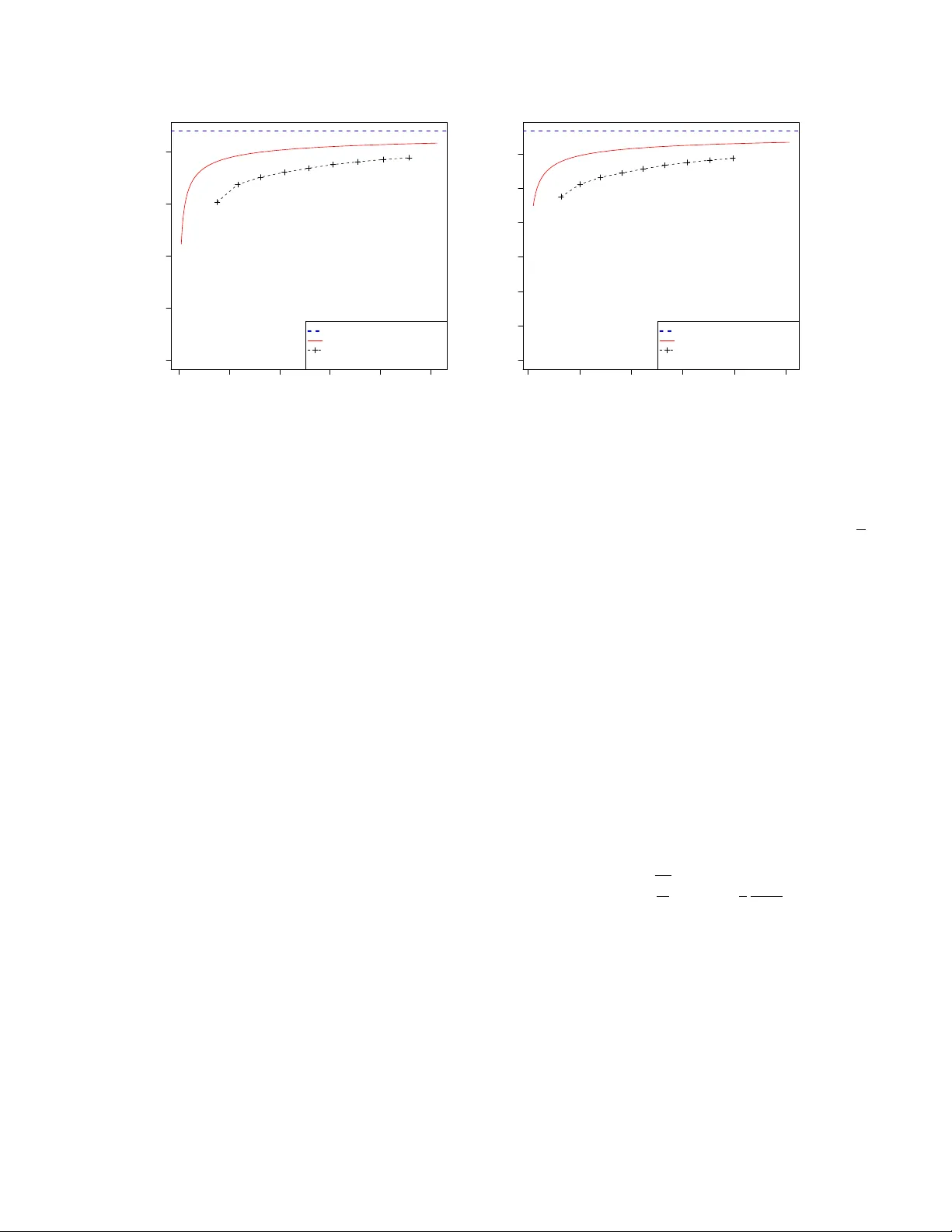
1 Least Squares Superposition Codes of Moderate Dictionary Size, Reliable at Rates up to Capacity Andre w R. Barron, Senior Member , IEEE, and Antony Joseph, Student Member , IEEE Submitted to IEEE T ransactions on Information Theory , June 4, 2010. Abstract —For the additive white Gaussian noise channel with av erage codeword power constraint, new coding methods are devised in which the codewords ar e sparse super positions, that is, linear combinations of subsets of vectors from a given design, with the possible messages indexed by the choice of subset. Decoding is by least squares, tailor ed to the assumed f orm of linear combination. Communication is shown to be reliable with error pr obability exponentially small f or all rates up to the Shannon capacity . I . I N T R O D U C T I O N The additiv e white Gaussian noise channel is basic to Shan- non theory and underlies practical communication models. W e introduce classes of superposition codes for this channel and analyze their properties. W e link theory and practice by showing superposition codes from polynomial size dictionaries with least squares decoding achie ve exponentially small error probability for any communication rate less than the Shannon capacity . A companion paper [7],[8] provides a fast decoding method and its analysis. The de velopments in v olve a mer ging of modern perspecti ves on statistical linear model selection and information theory . The familiar communication problem is as follows. An en- coder is required to map input bit strings u = ( u 1 , u 2 , . . . , u K ) of length K into codewords which are length n strings of real numbers c 1 , c 2 , . . . , c n , with norm expressed via the po wer (1 /n ) P n i =1 c 2 i . W e constrain the average of the po wer across the 2 K codew ords to be not more than P . The channel adds independent N (0 , σ 2 ) noise to the selected code word yielding a recei ved length n string Y . A decoder is required to map it into an estimate ˆ u which we want to be a correct decoding of u . Block error is the ev ent ˆ u 6 = u , bit error at position i is the ev ent ˆ u i 6 = u i , and the bit error rate is (1 /K ) P K i =1 1 { ˆ u i 6 = u i } . An analogous section error rate for our code is deﬁned below . The reliability requirement is that, with suf ﬁciently large n , the bit error rate or section error rate is small with high probability or , more stringently , the block error probability is small, averaged over input strings u as well as the distribution of Y . The communication rate R = K /n is the ratio of the input length to the codelength for communication across the channel. The supremum of reliable rates is the channel capacity C = (1 / 2) log 2 (1 + P /σ 2 ) , by traditional information theory as Andrew R. Barron and Antony Joseph are with the Department of Statistics, Y ale University , New Hav en, CT 06520 USA e-mail: { andrew .barron, antony .joseph } @yale.edu. Summary [9] of this paper was presented at the IEEE International Symposium on Information Theory , Austin, T exas, June 13-18, 2010. in [46], [29], [19]. Standard communication models, ev en in continuous-time, hav e been reduced to the above discrete-time white Gaussian noise setting, as in [29],[26]. This problem is also of interest in mathematics because of relationship to versions of the sphere packing problem as described in Conway and Sloane [16]. For practical coding the challenge is to achieve rates arbitrarily close to capacity with a codebook of moderate size, while guaranteeing reliable decoding in manageable computation time. W e introduce a new coding scheme based on sparse super- positions with a moderate size dictionary and analyze its per- formance. Least squares is the optimal decoder . Accordingly , we analyze the reliability of least squares and approximate least squares decoders. The analysis here is without concern for computational feasibility . In similar settings computational feasibility is addressed in the companion paper [7],[8], though the closeness to capacity at given reliability lev els is not as good as developed here. W e introduce sparse superposition codes and discuss the re- liability of least squares in Subsection I-A of this Introduction. Subsection I-B contrasts the performance of least squares with what is achieved by other methods of decoding. In Subsection I-C, we mention relations with work on sparse signal recovery in the high dimensional regression setting. Subsection I-D discusses other codes and Subsection I-E discusses some important forerunners to our de velopments here. Our reliability bounds are developed in subsequent sections. A. Sparse Superposition Codes W e dev elop the framework for code construction by lin- ear combinations. The story begins with a list (or book) X 1 , X 2 , . . . , X N of vectors, each with n coordinates, for which the codeword vectors tak e the form of superpositions β 1 X 1 + β 2 X 2 + . . . + β N X N . The vectors X j which are linearly combined provide the terms or components of the codew ords and the β j are the coefﬁcients. The receiv ed vector is in accordance with the statistical linear model Y = X β + ε where X is the matrix whose columns are the vec- tors X 1 , X 2 , . . . , X N and ε is the noise vector distributed Normal( 0 , σ 2 I ). In keeping with the terminology of that sta- tistical setting, the book X may be called the design matrix consisting of p = N v ariables, each with n observ ations, and this list of v ariables is also called the dictionary of candidate terms. 2 The coef ﬁcient vectors β are arranged to be of a speciﬁed form. F or subset superposition coding we arrange for a number L of the coordinates to be non-zero, with a speciﬁed positive value, and the message is con ve yed by the choice of subset. Denote B = N /L . If B is lar ge, it is a sparse superposition code . In this case, the number of terms sent is a small fraction of dictionary size. W ith some what greater freedom, one may arrange the non-zero coefﬁcients to be +1 or − 1 times a speciﬁed value, in which case the superposition code is said to be signed . Then the message is con veyed by the sequence of signs as well as the choice of subset. T o allow such forms of β , we do not in general take the set of permitted coefﬁcient vectors to be closed under a ﬁeld of linear operations, and hence our linear statistical model does not correspond to a linear code in the sense of traditional algebraic coding theory . In a specialization we call a partitioned superposition code , the book X is split into L sections of size B , with one term selected from each, yielding L terms in each code word out of a dictionary of size N = LB . Like wise, the coefﬁcient vector β is split into sections, with one coordinate non-zero in each section to indicate the selected term. Optionally , we hav e the additional freedom of choice of sign of this coefﬁcient, for a signed partitioned code. It is desirable that the section sizes be not larger than a moderate order polynomial in L or n , for then the dictionary is arranged to be of manageable size. Most con venient is the case that the sizes of these sections are powers of two. Then an input bit string of length K = L log 2 B splits into L substrings of size log 2 B . The encoder mapping from u to β is then obtained by interpreting each substring of u as simply giving the index of which coordinate of β is non-zero in the corresponding section. That is, each substring is the binary representation of the corresponding index. As we have said, the rate of the code is R = K/n input bits per channel uses and we arrange for R arbitrarily close to C . For the partitioned superposition code, this rate is R = ( L log B ) /n . For speciﬁed rate R , the codelength n = ( L/R ) log B . Thus, the length n and the number of terms L agree to within a log factor . W ith one term from each section, the number of possible codew ords 2 K is equal to B L = ( N/L ) L . Alternati vely , if we allo w for all subsets of size L , the number of possible codew ords would be  N L  , which is of order ( N e/L ) L = ( B e ) L , for L small compared to N . T o match the number of code words, it w ould correspond to reducing N by a factor of 1 /e . Though there would be the factor 1 /e savings in dictionary size from allowing all subsets of the speciﬁed size, the additional simplicity of implementation and simplicity of analysis with partitioned coding is such that we take advantage of it wherever appropriate. W ith signed partitioned coding the story is similar , now with (2 B ) L = (2 N /L ) L possible code words using the dictionary of size N = LB . The input string of length K = L log 2 (2 B ) = L (1 +log 2 B ) , splits into L sections with log 2 B bits to specify the non-zero term and 1 bit to specify its sign. For a rate R code this entails a codelength of n = ( L/R ) log(2 B ) . Control of the dictionary size is critical to computationally advantageous coding and decoding. Possible dictionary sizes are between the extremes K and 2 K dictated by the number and size of the sections, where K is the number of input bits. At one extreme, with 1 section of size B = 2 K , one has X as the whole codebook with its columns as the codew ords, but the exponential size makes its direct use impractical. At the other extreme we have L = K sections, each with two candidate terms in subset coding or two signs of a single term in sign coding with B = 1 ; in which case X is the generator matrix of a linear code. Between these extremes, we construct reliable, high-rate codes with codewords corresponding to linear combinations of subsets of terms in moderate size dictionaries. Design of the dictionary is guided by what is known from information theory concerning the distribution of symbols in the codew ords. By analysis of the conv erse to the channel coding theorem (as in [19]), for a reliable code at rate near capacity , with a uniform distribution on the sequence of input bits, the induced empirical distribution on coordinates of the codew ord must be close to independent Gaussian, in the sense that the resulting mutual information must be close to its maximum subject to the po wer constraint. W e dra w entries of X independently from a normal distri- bution with mean zero and a variance we specify , yielding the properties we want with high probability . Other distributions, such as independent equiprobable ± 1 , might also sufﬁce, with a near Gaussian shape for the code word distribution obtained by the con volutions associated with sums of terms in subsets of size L . For the vectors β , the non-zero coefﬁcients may be assigned to hav e magnitude p P /L , which with X ha ving independent entries of v ariance 1 , yields code words X β of average power near P . There is a freedom of scale that allo ws us to simplify the coefﬁcient representation. Henceforth, we arrange the coordinates of X j to ha ve variance P /L and set the non-zero coefﬁcients to ha ve magnitude 1 . Optimal decoding for minimal a verage probability of error consists of ﬁnding the codeword X β with coefﬁcient vector β of the assumed form that maximizes the posterior probability , conditioning on X and Y . This coincides, in the case of equal prior probabilities, with the maximum likelihood rule of seeking such a codew ord to minimize the sum of squared errors in ﬁt to Y . This is a least squares regression problem min β k Y − X β k 2 , with constraints on the coefﬁcient v ector . W e sho w for all R < C , that the least squares solution, as well as approximate least squares solutions such as may arise computationally , will have, with high probability , at most a negligible fraction of terms that are not correctly identiﬁed, producing a low bit error rate. The heart of the analysis shows that competing code words that dif fer in a fraction of at least α 0 terms are exponentially unlikely to hav e smaller distance from Y than the true codeword, provided that the section size B = L a is polynomially large in the number of sections L , where a sufﬁcient value of a is determined. For the partitioned superposition code there is a positiv e constant c such that for rates R less than the capacity C , with a positiv e gap ∆ = C − R not too large, the probability of a fraction of mistakes at least 3 0 200 400 600 800 1000 0.0 0.5 1.0 1.5 2.0 Blocklength, n Rate, R bits/ch. use Capacity PPV curve Superposition code (Partitioned) S N R = = 20 0 100 200 300 400 500 0.0 0.5 1.0 1.5 2.0 2.5 3.0 Blocklength, n Rate, R bits/ch. use Capacity PPV curve Superposition code (Partitioned) S N R = = 100 Fig. 1. Plot of comparison between achievable rates using our scheme and the theoretical best possible rates for block error probability of 10 − 4 and signal-to-noise ratio ( v ) values of 20 and 100. The curves for our partitioned superposition code were evaluated at points with number of sections L ranging from 20 to 100 in steps of 10, with corresponding B values taken to be L a v , where a v is as giv en in Lemma 4 later on. For the v values of 20 and 100 shown above, a v is around 2 . 6 and 1 . 6 , respectiv ely . α 0 is not more than exp {− nc min { ∆ 2 , α 0 }} . Consequently , for a target fraction of mistakes α 0 and target probability  , the required number of sections L or equi valently the codelength n = ( aL log L ) /R depends only polynomially on the reciprocal of the gap ∆ and on the reciprocal of α 0 . Indeed n of order [(1 /α 0 ) + (1 / ∆) 2 ] log(1 / ) suf ﬁces for the probability of the undesirable e vent to be less than  . Moreov er , an approach is discussed which completes the task of identifying the terms by arranging suf ﬁcient distance between the subsets, using composition with an outer Reed- Solomon (RS) code of rate near one. The Reed-Solomon code is arranged to have an alphabet of size B equal to a po wer of 2 . It is tailored to the partitioned code by ha ving the RS code symbols specify the terms selected from the sections. The outer RS code corrects the small fraction of remaining mistakes so that we end up not only with small section error rate but also with small block error probability . If R outer = 1 − δ is the rate of an RS code, with 0 < δ < 1 , then section error rate less than α 0 can be corrected, provided 2 α 0 < δ . Further , if R inner (or simply R ) is the rate associated with our inner (superposition) code, then the total rate after correcting for the remaining mistakes is gi ven by R total = R inner R outer . The end result, using our theory for the distribution of the fraction of mistakes of the superposition code, is that the block error probability is exponentially small. One may regard the composite code as a superposition code in which the subsets are forced to maintain at least a certain minimal separation, so that decoding to within a certain distance from the true subset implies exact decoding. Particular interest is giv en to the case that the rate R is made to approach the capacity C . Arrange R = C − ∆ n and α 0 = ∆ 2 n . One may let the rate gap ∆ n tend to zero (e.g. at a 1 / log n rate or any polynomial rate not faster than 1 / √ n ), then the overall rate R tot = (1 − 2 α 0 )( C − ∆ n ) continues to ha ve drop from capacity of order ∆ n , with the composite code having block error probability of order exp {− nc ∆ 2 n } . The e xponent abo ve, of order ( C − R ) 2 for R near C , is in agreement with the form of the optimal reliability bounds as in [28], [40], though here our constant c is not demonstrated to be optimal. In Figure 1 we plot curves of achiev able rates using our scheme for block error probability ﬁxed at 10 − 4 and signal to noise ratios of 20 and 100 . W e also compare this to a rate curve giv en in Polyanskiy , Poor and V erdu [40] (the PPV curve), where it is demonstrated that for a Gaussian channel with signal to noise ratio v , the block error probability  , codelength n and rate R with an optimal code can be well approximated by the following relation, R ≈ C − r V n Q − 1 (  ) + 1 2 log n n where V = ( v / 2)( v + 2) log 2 e/ ( v + 1) 2 is the channel dispersion and Q is the complementary Gaussian cumulative distribution function. For the superposition code curve, the y-axis gi ves the highest R comp for which the error probability stays below 10 − 4 . These curv es are based on the minimum of the bounds obtained by our lemma in Section III. W e see for the gi ven v and block error probability v alues, the achiev able rates using our scheme are reasonably close to the theoretically best scheme. Note that the PPV curve was computed with an approach that uses a codebook of size that is e xponential in blocklength, whereas our dictionary , of size LB , is of considerably smaller size. 4 B. Contrasting Methods of Decoding As we have said the least squares decoder minimizes || Y − X β || 2 with constraint on the form of coefﬁcient vector β . It is unkno wn whether approximate least squares decoding with rate R near the capacity C is practical in the equal power case studied here. Alternati ve methods include an iterati ve decoder that we discuss brieﬂy here and con vex optimization methods discussed here and in subsection I-C. The practical iterativ e decoder, for the partitioned super- position code, proposed and analyzed in [7],[8] is called an adaptive successive decoder . Decoding is broken into multiple steps, with the identiﬁcation of terms in a step achieved when the magnitude of the inner product between the corresponding X j ’ s and a computed residual vector is above a speciﬁed threshold. The residual vector for each step being obtained as the dif ference of Y and the contrib ution from columns decoded in previous steps. W ith a rate that is of order 1 / log B below capacity , the error probability attained there is exponentially small in L/ (log B ) 2 , to within a log log B factor . This error exponent is slightly smaller than the optimal n/ (log B ) 2 , obtained here by the least squares scheme. Moreover , as we saw above, the least squares decoder achiev es the optimal exponent for other orders ∆ n of drop from capacity . The sparse superposition codes achieving these performance lev els at rates near capacity , by least squares and by adapti ve successiv e decoding are dif ferent in an important aspect. For the present paper, we use a constant power allocation, with the same power P /L for each term. Howe ver in [7], to yield rates near capacity we needed a variable power allocation, achiev ed by a speciﬁc schedule of the non-zero β j ’ s. In contrast, if one were to use equal power allocation for the decoding scheme in [7], then reliable decoding holds only up to a threshold rate R 0 = (1 / 2) P / ( P + σ 2 ) , which is less than the capacity C , with the rate and capacity expressed in nats. The least squares optimization min || Y − X β || 2 is made challenging by the non-conv ex constraint that there be a speciﬁed number of non-zero coefﬁcients, one in each section. Nev ertheless, one can consider decoders based on projection to the con vex hull. This conv ex hull consists of the β vectors which have sum in each section equal to 1. (W ith signed cod- ing it becomes the constraint that the l 1 norm in each section is bounded by 1.) Geometrically , it pro vides a con ve x set of linear combinations in which the code words are the vertices. Decoding is completed with con ve x projection by moving to a vertex, e.g. with the largest coefﬁcient value in each section. This is a setting in which we initiated in vestigations, ho wev er, in that preliminary analysis, we found that such l 1 constrained quadratic optimization allows for successful decoding only for rates up to R thres for the equal power case. It is as yet unclear what its reliability properties would be at rates up to capacity C with variable po wer . C. Related W ork on Sparse Signal Recovery The conclusions regarding communication rate may be also expressed in the language of sparse signal r ecovery and com- pr essed sensing . A number of terms selected from a dictionary is linearly combined and subject to noise in accordance with the linear model framew ork Y = X β +  . Let N be the number of variables and L the number of non-zero terms. An issue dealt with by these ﬁelds, is the minimal number of observ ations n suf ﬁcient to reliably recover the terms. In our setting, the non-zero values of the coef ﬁcients are known and n satisﬁes the relationship n = (1 /R ) log  N L  for general subsets and n = (1 /R ) L log( N/L ) for the partitioned case. W e show that reliable recovery is possible provided R < C . The conclusions here complement recent work on sparse signal recovery [14],[20], [22] in the sparse noise case and [49],[48],[50],[24],[47],[13] in the Gaussian noise case. Con- nections between signal recovery and channel coding are also highlighted in [47]. A hallmark of work in signal reco very is allow ance for greater generality of signal coefﬁcient values. In the regime as treated here, where N  L and where there is a control on the sum of squares of the coefﬁcients as well as a control on the minimum coefﬁcient value, conclusions from this literature take the form that the best n is of the order L log( N /L ) , with upper and lo wer bounds on the constants deriv ed. It is natural to call (the reciprocal of) the best constant, for a given set of allowed signals and giv en noise distribution, the compr essed sensing capacity or signal r ecovery capacity . For the conv erse results in [48],[50], Fano’ s inequality is used to establish constants related to the channel capacity . Reﬁnements of this w ork can be found in [24]. Conv ex projection methods with l 1 constraints as in [49],[47],[13], hav e been used for achie vability results. The same order of performance is achiev ed by a maximum correlation estimator [24]. Analysis of constants achieved by least squares is in [48], [23]. The above analysis, when interpreted in our setting, correspond to saying that these schemes have communication rate that is positiv e, though at least a ﬁxed amount below the channel capacity . For our setting, a consequence of the result here is that the signal recovery capacity is equal to the channel capacity . D. Related Communication Issues and Schemes The de velopment here is speciﬁc to the discrete-time chan- nel for which Y i = c i + ε i for i = 1 , 2 , . . . , n with real- valued inputs and outputs and with independent Gaussian noise. Standard communication models, ev en in continuous- time, ha ve been reduced to this discrete-time white Gaussian noise setting, or to parallel uses of such, when there is a frequency band constraint for signal modulation and when there is a speciﬁed spectrum of noise ov er that frequency band, as in [29], [26]. Standard approaches, as discussed in [26], entail a decom- position of the problem into separate problems of coding and of shaping of a multiv ariate signal constellation. F or the low signal-to-noise re gime, binary codes sufﬁce for communication near capacity and there is no need for shaping. There is prior work concerning reliable communications near capacity for certain discrete input channels. Iterativ e decoding algorithms based on statistical belief propagation in loopy networks have been empirically sho wn in v arious works to provide reliable and moderately fast decoding at rates near the capacity for 5 such channels, and mathematically prov en to provide such properties in certain special cases, such as the binary erasure channel in [37], [38]. These include codes based on lo w density parity check codes [28] and turbo codes [11], [12]. See [43],[44] for some aspects of the state of the art with such techniques. A different approach to reliable and computationally feasi- ble decoding to achieve the rates possible with restriction to discrete alphabet signaling, is in the work on channel polariza- tion of Arikan and T elatar [3], [4]. They achie ve rates up to the mutual information I between a uniform input distribution and the output of the channel. Error probability is demonstrated there at a lev el exponentially small in n 1 / 2 for any ﬁxed R < I . In contrast for our codes the error probability is exponentially small in n ( C − R ) 2 for the least squared decoder and within a log factor of being exponentially small in n for the practical decoder in [7], [8]. Moreover , communication is permitted at higher rates beyond that associated with a uniform input distribution. W e are aware from personal con versation with Imre T elatar and Emanuel Abbe that they are in vestigating the extent to which channel polarization can be adapted to Gaussian signaling. In the high signal-to-noise regime, one needs a greater signal alphabet size. As explained in [26], along with coding schemes on such alphabets, additional shaping is required in order to be able to achieve rates up to capacity . Here shaping refers to making the codewords vectors approximate a good packing of points on the n dimensional sphere of square radius dictated by the power . An implication is that, marginally and jointly for any subset of codeword coordinates, the set of codewords should have empirical distribution not far from Gaussian. Notice that we b uild shaping directly into the coding scheme by the superposition strate gy yielding codew ords following a Gaussian distribution. Our ideas of sparse superposition coding are adapted to Gaussian vector quantization in, Kontoyiannis, Gitzenis and Rad [34]. Applicability to vector quantization is natural be- cause of the abov e-mentioned connection between packing and coding. E. Precur sors The analysis of concatenated codes in Forney [25] is an important forerunner to the dev elopment we giv e here. He identiﬁed beneﬁts of an outer Reed-Solomon code paired in theory with an optimal inner code of Shannon-Gallager type and in practice with binary inner codes based on linear combinations of orthogonal terms (for target rates K /n less than 1 such a basis is av ailable). The challenge concerning theoretically good inner codes is that the number of messages searched is exponentially large in the inner codelength. Forney made the inner codelength of logarithmic size compared to the outer codelength as a step tow ard practical solution. Howe ver , caution is required with such a strategy . Suppose the rate of the inner code has only a small drop from capacity , ∆ = C − R . For small inner code error probability , the inner codelength must be of order at least 1 / ∆ 2 . So with that scheme one has the undesirable consequence that the required outer codelength becomes exponential in 1 / ∆ 2 . For the Gaussian noise channel, our tactic to o vercome that difﬁculty uses a superposition inner code with a polynomial size dictionary . W e use inner and outer codelengths that are comparable, with the outer code used to correct errors in a small fraction of the sections of the inner code. The o verall codelength to achieve error probability  remains of the order (1 / ∆ 2 ) log(1 / ) . Another point of relationship of this w ork with other ideas is the problem of multiple comparisons in hypothesis tests. False discovery rate [10] for a giv en signiﬁcance le vel, rather than exclusi vely ov erall error probability is a recent focus in statistical de velopment, appropriate when considering very large numbers of hypotheses as arise with many variables in regression. Our theory for the distribution of the fraction of incorrectly determined terms (associated with bit error rate rather than block error rate) pro vides an additional glimpse of what is possible in a regression setting with a large number of subset hypotheses. The work of [32] is a recent e xample where subset selection within groups (sections) of variables is addressed by extension of false discovery methods. The idea of superposition coding for Gaussian noise chan- nels began with Cover [18] in the context of multiple-user channels. In that setting what is sent is a sum of codewords, one for each message. Here we are putting that idea to use for the original Shannon single-user problem. The purpose here of computational feasibility is dif ferent from the original multi- user purpose which was identiﬁcation of the set of achiev able rates. Another connection with that broadcast channel work by Cov er is that for such Gaussian channels, the power allocation can be arranged such that messages can be peeled off one at a time by successiv e decoding. Related rate splitting and successiv e decoding for superposition codes are developed for Gaussian multiple-access problems in [15] and [45], where in some cases to establish such reductions, rate splitting is applied to individual users. Howe ver , feasibility has been lack- ing in part due to the absence of demonstration of reliability at high rate with superpositions from polynomial size code designs. It is an attracti ve feature of our solution for the single-user channel that it should be amenable to extension to practical solution of the corresponding multi-user channels, namely , the Gaussian multiple access and Gaussian broadcast channel. Section II contains brief preliminaries. Section III provides core lemmas on the reliability of least squares for our super - position codes. Section IV analyzes the matter of section size sufﬁcient for reliability . Section V conﬁrms that the probability of more than a small fraction of mistakes is exponentially small. Section VI discusses properties of the composition of our code with a binary outer code for correction of any remaining small fraction of mistakes. The appendix collects some auxiliary matters. I I . P R E L I M I N A R I E S For vectors a, b of length n , let k a k 2 be the sum of squares of coordinates, let | a | 2 = (1 /n ) P n i =1 a 2 i be the a verage square and let a · b = (1 /n ) P n i =1 a i b i be the associated inner product. It is a matter of taste, but we ﬁnd it slightly more conv enient to work henceforth with the norm | a | rather than k a k . 6 Concerning the base of the logarithm ( log ) and associated exponential ( exp ), base 2 is most suitable for interpretation and base e most suitable for the calculus. For instance, the rate R = ( L log B ) /n is measured in bits if the log is base 2 and nats if the log is base e . T ypically , conclusions are stated in a manner that can be interpreted to be in variant to the choice of base, and base e is used for conv enience in the deriv ations. W e make repeated use of the follo wing moment generating function and its associated large de viation exponent in con- structing bounds on error probabilities. If Z and ˜ Z are normal with means equal to 0 , variances equal to 1 , and correlation coefﬁcient ρ then E ( e ( λ/ 2)( Z 2 − ˜ Z 2 ) ) takes the value 1 / [1 − λ 2 (1 − ρ 2 )] 1 / 2 when λ 2 < 1 / (1 − ρ 2 ) and inﬁnity otherwise. So the asso- ciated cumulant generating function of (1 / 2)( Z 2 − ˜ Z 2 ) is − (1 / 2) log(1 − λ 2 (1 − ρ 2 )) , with the understanding that the minus log is replaced by inﬁnity when λ 2 is at least 1 / (1 − ρ 2 ) . For positiv e ∆ we deﬁne the quantity D = D (∆ , 1 − ρ 2 ) giv en by D = max λ ≥ 0  λ ∆ + (1 / 2) log(1 − λ 2 (1 − ρ 2 ))  . This D matches the relativ e entropy D ( p ∗ k p ) between biv ariate normal densities, where p ( z , ˜ z ) is the joint density of Z, ˜ Z of correlation ρ and where p ∗ ( z , ˜ z ) is the joint normal obtained by tilting that density by e ( λ/ 2)( z 2 − ˜ z 2 ) , chosen to make (1 / 2)( Z 2 − ˜ Z 2 ) hav e mean ∆ , when there is such a λ . Let’ s gi ve D (∆ , 1 − ρ 2 ) explicitly as an increasing function of the ratio ∆ 2 / (1 − ρ 2 ) . W orking with logarithm base e , the deriv ativ e with respect to λ of the expression being maximized yields a quadratic equation which can be solv ed for the optimal λ ∗ = 1 2∆  p 1 + 4∆ 2 / (1 − ρ 2 ) − 1  . Let q = 4∆ 2 / (1 − ρ 2 ) and γ = √ 1 + q − 1 , which is near q / 2 when q is small and approximately √ q when q is large. Plug the optimized λ into the abov e expression and simplify to obtain D = (1 / 2)  γ − log (1 + γ / 2)  , which is at least γ / 4 . Thus D is the composition of strictly increasing non- negati ve functions (1 / 2)  γ − log(1 + γ / 2)  and γ = √ 1 + q − 1 ev aluated at q = 4∆ 2 / (1 − ρ 2 ) . For small values of this ratio, we see that D is near q / 8 = (1 / 2)∆ 2 / (1 − ρ 2 ) . The expression corresponding to D but with the maximum restricted to 0 ≤ λ ≤ 1 is denoted D 1 = D 1 (∆ , 1 − ρ 2 ) , that is, D 1 = max 0 ≤ λ ≤ 1  λ ∆ + (1 / 2) log(1 − λ 2 (1 − ρ 2 ))  . The corresponding optimal value of λ is min { 1 , λ ∗ } . When the optimal λ is less than 1 , the v alue of D 1 matches D as giv en abo ve. The λ = 1 case occurs when 1 + 4∆ 2 / (1 − ρ 2 ) ≥ (1 + 2∆) 2 , or equiv alently ∆ ≥ (1 − ρ 2 ) /ρ 2 . Then the exponent is D 1 = ∆ + (1 / 2) log ρ 2 , which is as least ∆ − (1 / 2) log (1 + ∆) . Consequently , in this regime D 1 is between ∆ / 2 and ∆ . The special case ρ 2 = 1 is included with D 1 = ∆ . I I I . P E R F O R M A N C E O F L E A S T S Q UA R E S As we ha ve said, least squares provides optimal decoding of superposition codes. In this section we examine the per- formance of this least squares choice in terms of rate and reliability . W e focus on partitioned superposition codes in which the code words are superpositions with one term from each section. Let S be an allowed subset of terms. W e examine ﬁrst subset coding in which to each such S there is a corresponding coefﬁcient vector β in which the non-zero coefﬁcients take a speciﬁed positi ve value as discussed abov e. W e may denote the corresponding code word X S = X β . Among such code words, least squares provides a choice for which | Y − X S | 2 is minimal. For a subset S of size L we measure how dif ferent it is from S ∗ , the subset that was sent. Let ` = car d ( S − S ∗ ) be the number of entries of S not in S ∗ . Equivalently , since S and S ∗ are of the same size, it is the number of entries of S ∗ not in S . Let ˆ S be the least squares solution, or an approximate least squares solution, achieving | Y − X ˆ S | 2 ≤ | Y − X S ∗ | 2 + δ 0 with δ 0 ≥ 0 . W e call card ( ˆ S − S ∗ ) the number of mistakes. Indeed, for a partitioned superposition code it is the number of sections incorrectly decoded. There is a role for the function C α = 1 2 log(1 + αv ) for 0 ≤ α ≤ 1 , where v = P /σ 2 is the signal-to-noise ratio and C 1 = C = (1 / 2) log(1 + v ) is the channel capacity . W e note that C α − αC is a non-neg ativ e concave function equal to 0 when α is 0 or 1 and strictly positiv e in between. The quantity C α − αR is larger by the additional amount α ( C − R ) , positive when the rate R is less than the Shannon capacity C . The function ψ α ( λ ) = − (1 / 2) log[1 − λ 2 αv / (1 + αv )] with 0 ≤ λ ≤ 1 is the cumulant generating function of a test statistic in our analysis. Our ﬁrst result on the distribution of the number of mistakes is the following. Lemma 1: Set α = `/L for an ` ∈ { 1 , 2 , . . . , L } . For approx- imate least squares with 0 ≤ δ 0 ≤ 2 σ 2 ( C α − αR ) / log e , the probability of a fraction α = `/L mistakes is upper bounded by  L αL  exp  − n max 0 ≤ λ ≤ 1  λ ∆ α − ψ α ( λ )   , or equiv alently ,  L αL  exp {− nD 1 (∆ α , αv / (1 + αv )) } , where ∆ α = C α − αR − ( δ 0 / 2 σ 2 ) log e and v is the signal- to-noise ratio. Remark 1: W e ﬁnd this Lemma 1 to be especially useful for α in the lower range of the interval from 0 to 1 . Lemma 2 below will reﬁne the analysis to provide an exponent more useful in the upper range of the interval. Proof of Lemma 1: T o incur ` mistakes, there must be an allowed subset S of size L which differs from the subset S ∗ sent in an amount car d ( S − S ∗ ) = car d ( S ∗ − S ) = ` which 7 undesirably has squared distance | Y − X S | 2 less than or equal to the value | Y − X S ∗ | 2 + δ 0 achiev ed by S ∗ . The analysis proceeds by considering an arbitrary such S , bounding the probability that | Y − X S | 2 ≤ | Y − X S ∗ | 2 + δ 0 , and then using an appropriately designed union bound to put such probabilities together . Consider the statistic T = T ( S ) gi ven by T ( S ) = 1 2  | Y − X S | 2 σ 2 − | Y − X S ∗ | 2 σ 2  . W e set a threshold for this statistic equal to t = δ 0 / (2 σ 2 ) . The ev ent of interest is that T ≤ t . The subsets S and S ∗ hav e an intersection S 1 = S ∩ S ∗ of size L − ` and difference S 2 = S − S 1 of size ` = αL . Giv en ( X j : j ∈ S ) the actual density of Y is normal with mean X S 1 = P j ∈ S 1 X j and variance ( σ 2 + αP ) I and we denote this density p ( Y | X S 1 ) . In particular , there is conditional independence of Y and X S 2 giv en X S 1 . Consider the alternative hypothesis of a conditional distri- bution for Y giv en X S 1 and X S 2 which is Normal( X S , σ 2 I ). It is the distribution which would have governed Y if S were sent. Let p h ( Y | X S 1 , X S 2 ) = p h ( Y | X S ) be the associated conditional density . W ith respect to this alternative hypoth- esis, the conditional distribution for Y giv en X S 1 remains Normal( X S 1 , ( σ 2 + α P ) I ). That is, p h ( Y | X S 1 ) = p ( Y | X S 1 ) . W e decompose the abov e test statistic as 1 2  | Y − X S 1 | 2 σ 2 + αP − | Y − X S ∗ | 2 σ 2  + 1 2  | Y − X S | 2 σ 2 − | Y − X S 1 | 2 σ 2 + αP  . Let’ s call the two parts of this decomposition T 1 and T 2 , respectiv ely . Note that T 1 = T 1 ( S 1 ) depends only on terms in S ∗ , whereas T 2 = T 2 ( S ) depends also on the part of S not in S ∗ . Concerning T 2 , note that we may express it as T 2 ( S ) = 1 n log p ( Y | X S 1 ) p h ( Y | X S ) + C α , where C α = 1 2 log σ 2 + αP σ 2 is the adjustment by the logarithm of the ratio of the normal- izing constants of these densities. Thus T 2 is equiv alent to a likelihood ratio test statistic between the actual conditional density and the constructed alternativ e hypothesis for the conditional density of Y giv en X S 1 and X S 2 . It is helpful to use Bayes rule to pro- vide p h ( X S 2 | Y , X S 1 ) via the equality of p h ( X S 2 | Y ,X S 1 ) p ( X S 2 | X S 1 ) and p h ( Y | X S 1 ,X S 2 ) p ( Y | X S 1 ) and to interpret this equality as providing an alternativ e representation of the likelihood ratio in terms of the rev erse conditionals for X S 2 giv en X S 1 and Y . W e are examining the event E ` that there is an allowed subset S = S 1 ∪ S 2 (with S 1 = S ∩ S ∗ of size L − ` and S 2 = S − S 1 of size ` ) such that that T ( S ) is less than t . For positiv e λ the indicator of this e vent satisﬁes 1 E ` ≤ X S 1 X S 2 e − n ( T ( S ) − t ) ! λ , because, if there is such an S with T ( S ) − t negati ve, then indeed that contributes a term on the right side of value at least 1 . Here the outer sum is over S 1 ⊂ S ∗ of size L − ` . For each such S 1 , for the inner sum, we hav e ` sections in each of which, to comprise S 2 , there is a term selected from among B − 1 choices other than the one prescribed by S ∗ . T o bound the probability of E ` , take the expectation of both sides, bring the expectation on the right inside the outer sum, and write it as the iterated e xpectation, where on the inside condition on Y , X S 1 and X S ∗ to pull out the factor in volving T 1 , to obtain that P [ E ` ] is not more than X S 1 E e − nλ ( T 1 ( S 1 ) − t ) E X S 2 | Y ,X S 1 ,X S ∗ X S 2 e − nT 2 ( S ) ! λ . A simpliﬁcation here is that the true density for X S 2 is independent of the conditioning v ariables Y , X S 1 and X S ∗ . W e arrange for λ to be not more than 1 . Then by Jensen’ s inequality , the conditional expectation may be brought inside the λ power and inside the inner sum, yielding P [ E ` ] ≤ X S 1 E e − nλ ( T 1 ( S 1 ) − t ) X S 2 E X S 2 | Y ,X S 1 e − nT 2 ( S ) ! λ . Recall that e − nT 2 ( S ) = p h ( X S 2 | Y , X S 1 ) p ( X S 2 ) e − nC α and that the true density for X S 2 is independent of the conditioning v ariables in accordance with the p ( X S 2 ) in denominator . So when we take the expectation of this ratio we cancel the denominator lea ving the numerator density which integrates to 1 . Consequently , the resulting expectation of e − nT 2 ( S ) is not more than e − nC α . The sum over S 2 entails less than B ` = e nR`/L choices so the bound is P [ E ` ] ≤ X S 1 E e − nλT 1 ( S 1 ) e − nλ [ C α − αR − t ] . Now nT 1 ( S 1 ) is a sum of n independent mean-zero random variables each of which is the difference of squares of normals for which the squared correlation is ρ 2 α = 1 / (1 + αv ) . So the e xpectation E e − nλT 1 ( S 1 ) is found to be equal to [1 / [1 − λ 2 αv / (1 + αv )]] n/ 2 . When plugged in above it yields the claimed bound optimized ov er λ in [0 , 1] . W e recognize that the exponent takes the form D 1 (∆ , 1 − ρ 2 ) with 1 − ρ 2 = αv / (1+ αv ) as discussed in the preliminaries. This completes the proof of Lemma 1. Some additional remarks: The exponent D 1 in Lemma 1 (and its reﬁnement in Lemma 2 to follow) depends on the fraction of mistakes α and the signal-to-noise ratio v only through ∆ α = C α − αR − t and 1 − ρ 2 α . As we ha ve seen, the λ < 1 case occurs when ∆ α < (1 − ρ 2 α ) /ρ 2 α and then D is near (1 / 2)∆ 2 α / (1 − ρ 2 α ) when it is small; whereas, the λ = 1 case 8 occurs when ∆ α ≥ (1 − ρ 2 α ) /ρ 2 α and then the exponent is as least ∆ α − (1 / 2) log(1 + ∆ α ) ≥ ∆ α / 2 . This behavior of the exponent is similar to the usual order ( C − R ) 2 for R close to C and order C − R for R farther from C associated with the theory in Gallager [29]. A difﬁculty with the Lemma 1 bound is that for α near 1 and for R correspondingly close to C , in the key quantity ∆ 2 α / (1 − ρ 2 α ) , the order of ∆ 2 α is (1 − α ) 2 , which is too close to zero to cancel the effect of the combinatorial coefﬁcient. The following lemma reﬁnes the analysis of Lemma 1, obtaining the same exponent with an improv ed correlation coefﬁcient. The denominator 1 − ρ 2 α = α (1 − α ) / (1 + αv ) is improv ed by the presence of the f actor (1 − α ) allo wing the conclusion to be useful also for α near 1 . The price we pay is the presence of an additional term in the bound. For the statement of Lemma 2 we again use the test statistic T ( S ) as deﬁned in the proof of Lemma 1. For interpretation of what follo ws with arbitrary base of logarithm, in that deﬁnition of T ( S ) multiply by log e and like wise take the threshold to be t = δ 0 2 σ 2 log e . Lemma 2: Let a positive integer ` ≤ L be gi ven and let α = `/L . Suppose 0 ≤ t < C α − αR . As abov e let E ` be the ev ent that there is an allowed L term subset S with S − S ∗ of size ` such that T ( S ) is less than t . Then P [ E ` ] is bounded by the minimum for t α in the interval between t and C α − αR of the following  L Lα  exp  − nD 1 ( C α − αR − t α , 1 − ρ 2 α )  + exp  − nD ( t α − t, α 2 v / (1 + α 2 v )]  . where 1 − ρ 2 α = α (1 − α ) v / (1 + αv ) . Proof of Lemma 2: Split the test statistic T ( S ) = ˜ T ( S ) + T ∗ where ˜ T ( S ) = 1 2  | Y − X S | 2 σ 2 − | Y − (1 − α ) X S ∗ | 2 σ 2 + α 2 P  and T ∗ = 1 2  | Y − (1 − α ) X S ∗ | 2 σ 2 + α 2 P − | Y − X S ∗ | 2 σ 2  Like wise we split the threshold t = ˜ t + t ∗ where t ∗ = − ( t α − t ) is negati ve and ˜ t = t α is positiv e. The e vent that there is an S with T ( S ) < t is contained in the union of the two ev ents ˜ E ` , that there is an S with ˜ T ( S ) < ˜ t , and the ev ent E ∗ ` , that T ∗ < t ∗ . The part T ∗ has no dependence on S so it can be treated more simply . It is a mean zero av erage of differences of squared normal random variables, with squared correlation 1 / (1 + α 2 v ) . So using its moment generating function, P [ E ∗ ` ] is exponentially small, bounded by the second of the two expressions abo ve. Concerning P [ ˜ E ` ] , its analysis is much the same as for Lemma 1. W e again decompose ˜ T ( S ) as the sum ˜ T 1 ( S 1 ) + ˜ T 2 ( S ) , where ˜ T 2 ( S ) = T 2 ( S ) is the same as before. The 0 20 40 60 80 α α error exponents 0 α α 0 0.2 0.4 0.6 0.8 1 P(# mistakes >l 0 ) = 1.8(10) −12 L = 100 B = 8192 P/ σ σ 2 = = 15 C = 2 R = 0.7C n = 929 N = 819200 −logP(E l ~ ) −logP(E * l ) d n, α α Fig. 2. Exponents of contributions to the error probability as functions of α = `/L using exact least squares, i.e., t = 0 , with L = 100 , B = 2 13 , signal- to-noise ratio v = 15 , and rate 70% of capacity . The red and blue curves are the − log P [ ˜ E ` ] and − log P [ E ∗ ` ] bounds, using the natural logarithm, from the two terms in Lemma 2 with optimized t α . The dotted green curve is d n,α explained below . With α 0 = 0 . 1 , the total probability of at least that fraction of mistakes is bounded by 1 . 8(10) − 12 . difference is that in forming ˜ T 1 ( S 1 ) we subtract | Y − (1 − α ) X S ∗ | 2 σ 2 + α 2 P rather than | Y − X S ∗ | 2 σ 2 . Consequently , ˜ T 1 ( S 1 ) = 1 2  | Y − X S 1 | 2 σ 2 + αP − | Y − (1 − α ) X S ∗ | 2 σ 2 + α 2 P  , which again in volves a dif ference of squares of standardized normals. But here the coefﬁcient (1 − α ) multiplying X S ∗ is such that we have maximized the correlations between the Y − X S 1 and Y − (1 − α ) X S ∗ . Consequently , we have reduced the spread of the distrib ution of the dif ferences of squares of their standardizations as quantiﬁed by the cumulant generating function. One ﬁnds that the squared correlation coefﬁcient is ρ 2 α = (1+ α 2 v ) / (1+ αv ) for which 1 − ρ 2 α = α (1 − α ) v / (1 + αv ) . Accordingly we have that the moment generating function is E e − nλ ˜ T ( S 1 ) = exp {− ( n/ 2) log[1 − λ 2 (1 − ρ 2 α )] } which giv es rise to the bound appearing as the ﬁrst of the two expressions abov e. This completes the proof of Lemma 2. The method of analysis also allows consideration of subset coding without partitioning. For , in this case all  N L  subsets of size L correspond to codew ords, so with the rate in nats we hav e e nR =  N L  . The analysis proceeds in the same manner , with the same number  L L − `  of choices of sets S 1 = S ∩ S ∗ where S and S ∗ agree on L − ` terms, but no w with  N − L `  choices of sets S 2 = S − S ∗ of size ` where they disagree. W e obtain the same bounds as above e xcept that where we hav e B ` = e nαR with the exponent αR it is replaced by  N − L `  = e nR ( α ) with the exponent R ( α ) deﬁned by R ( α ) = R log  N − L αL  / log  N L  . Thus we have the following conclusion. 9 Corollary 3: For subset superposition coding, the proba- bility of the ev ent E ` that there is a β that is incorrect in ` sections and has | Y − X β | 2 ≤ | Y − X β ∗ | 2 + δ 0 is bounded by the minimum of the same expressions given in Lemma 1 and Lemma 2 except that the term αR appearing in these expression be replaced by the quantity R ( α ) deﬁned abo ve. I V . S U FFI C I E N T S E C T I O N S I Z E W e come to the matter of suf ﬁcient conditions on the section size B for our exponential bounds to swamp the combinatorial coefﬁcient, for partitioned superposition codes. W e call a = (log B ) / (log L ) the section size rate , that is, the bits required to describe the member of a section relati ve to the bits required to describe which section. It is in variant to the base of the log. Equiv alently we ha ve B and L related by B = L a . Note that the size of a controls the polynomial size of the dictionary N = B L = L a +1 . In both cases the codelength may be written as n = aL log L R . W e do not want a requirement on the section sizes with a of order 1 / ( C − R ) for then the complexity would grow exponentially with this in verse of the gap from capacity . So instead let’ s decompose 4 α = ˜ 4 α + α ( C − R ) − t α where ˜ 4 α = C α − αC . W e inv estigate in this section the use of ˜ 4 α to swamp the combinatorial coefﬁcient. In the next section excess in ˜ 4 α , beyond that needed to cancel the combinatorial coefﬁcient, plus α ( C − R ) − t α are used to produce exponentially small error probability . Deﬁne D α,v = D 1 ( 4 α , 1 − ρ 2 α ) and ˜ D α,v = D 1 ( ˜ ∆ α , 1 − ρ 2 α ) . Now D 1 (∆ , 1 − ρ 2 ) is increasing as a function of ∆ , so D α,v is greater than ˜ D α,v whenev er 4 α > ˜ 4 α . Accordingly , we decompose the exponent D α,v as the sum of two components, namely , ˜ D α,v and the difference D α,v − ˜ D α,v . W e then ask whether the ﬁrst part of the exponent denoted ˜ D α,v is suf ﬁcient to wash out the af fect of the log combina- torial coefﬁcient log  L Lα  . That is, we want to arrange for the nonnegati vity of the difference d n,α = n ˜ D α,v − log  L Lα  . This dif ference is small for α near 0 and 1 . Furthermore, its constituent quantities hav e a shape comparable to multiples of α (1 − α ) . Consider ﬁrst ˜ 4 α = C α − α C and take the log to be base e . It has second deri vati ve − (1 / 2) v 2 / (1 + αv ) 2 . It follows that ˜ 4 α ≥ (1 / 4) α (1 − α ) v 2 / (1 + v ) 2 , since the difference of the two sides has negati ve second deri vati ve, so it is concave and equals 0 at α = 0 and α = 1 . Likewise (1 − ρ 2 α ) = α (1 − α ) v/ (1 + αv ) so the ratio ˜ u = 4 ˜ 4 2 α / (1 − ρ 2 α ) is at least (1 / 4) α (1 − α ) v 3 (1 + αv ) / (1 + v ) 4 . Consequently , whether the optimal λ is equal to 1 or is less than 1 , we ﬁnd that ˜ D α,v is of order α (1 − α ) . Similarly , there is the matter of log  L Lα  , with Lα re- stricted to hav e integer values. It enjoys the upper bounds min( α, 1 − α ) L log L and L log 2 so that it is not more than α (1 − α )( L log L ) / (1 − δ L ) where δ L = (log 2) / log L . Consequently , using n = ( aL log L ) /R , one ﬁnds that for sufﬁciently large a depending on v , the difference d n,α is nonnegati ve uniformly for the permitted α in [0 , 1] . The smallest such section size rate is a v ,L = max α R log  L Lα  ˜ D α,v L log L , where the maximum is for α in { 1 /L, 2 /L, . . . , 1 − 1 /L } . This deﬁnition has the required in v ariance to the choice of base of the logarithm, assuming that the same base is used for the communication rate R and for the C α − αC that arises in the deﬁnition of ˜ D α,v . In the above ratio the numerator and denominator are both 0 at α = 0 and α = 1 (yielding d n,α = 0 at the ends). Accordingly , we have excluded 0 and 1 from the deﬁnition of a v ,L for ﬁnite L . Nev ertheless, limiting ratios arise at these ends. W e show that the v alue of a v ,L is fairly insensiti ve to the value of L , with the maximum over the whole range being close to a limit a v which is characterized by values in the vicinity of α = 1 . Let v ∗ near 15 . 8 be the solution to (1 + v ∗ ) log(1 + v ∗ ) = 3 v ∗ log e. Lemma 4: The section size rate a v ,L has a continuous limit a v = lim L →∞ a v ,L which is given, for 0 < v < v ∗ , by a v = R [(1 + v ) log (1 + v ) − v log e ] 2 / [8 v (1 + v ) log e ] and for v ≥ v ∗ by a v = R [(1 + v ) log (1 + v ) − 2 v log e ] / [2(1 + v )] where v is the signal-to-noise ratio. W ith R replaced by C = (1 / 2) log(1 + v ) and using log base e, in the case 0 < v < v ∗ , it is 4 v (1 + v ) log(1 + v ) [(1 + v ) log (1 + v ) − v ] 2 which is approximately 16 /v 2 for small positi ve v ; whereas, in the case v ≥ v ∗ it is (1 + v ) log (1 + v ) (1 + v ) log (1 + v ) − 2 v which asymptotes to the v alue 1 for lar ge v . Proof of Lemma 4: For α in (0 , 1) we use log  L Lα  ≤ L log 2 and the strict positivity of ˜ D α,v to see that the ratio in the deﬁnition of a v ,L tends to zero uniformly within compact sets interior to (0 , 1) . So the limit a v is determined by the maximum of the limits of the ratios at the two ends. In the vicinity of the left and right ends we replace log  L Lα  by the continuous upper bounds αL log L and (1 − α ) L log L , respectiv ely , which are tight at α = 1 /L and 1 − α = 1 /L , respectiv ely . Then in accordance with L ’Hopital’ s rule, the limit of the ratios equals the ratios of the deriv ati ves at α = 0 and α = 1 , respecti vely . Accordingly , a v = max ( R ˜ D 0 0 ,v , − R ˜ D 0 1 ,v ) , 10 where ˜ D 0 0 ,v and ˜ D 0 1 ,v are the deri vati ves of ˜ D α,v with respect to α ev aluated at α = 0 and α = 1 , respecti vely . T o determine the behavior of ˜ D α = ˜ D α,v in the vicinity of 0 and 1 we ﬁrst need to determine whether the optimal λ in its deﬁnition is strictly less than 1 or equal to 1 . According to our earlier dev elopments that is determined by whether ˜ ∆ α < (1 − ρ 2 α ) /ρ 2 α . The right side of this is α (1 − α ) v / (1 + α 2 v ) . So it is equiv alent to determine whether the ratio ( C α − αC )(1 + α 2 v ) α (1 − α ) v is less than 1 for α in the vicinity of 0 and 1 . Using L ’Hopital’ s rule it sufﬁces to determine whether the ratio of deri v ati ves is less than 1 when ev aluated at 0 and 1 . At α = 0 it is (1 / 2)[ v − log(1 + v )] /v which is not more than 1 / 2 (certainly less than 1 ) for all positi ve v ; whereas, at α = 1 the ratio of deriv ativ es is (1 / 2)[(1 + v ) log(1 + v ) − v ] /v which is less than 1 if and only if v < v ∗ . For the cases in which the optimal λ < 1 , we need to determine the deriv ati ve of ˜ D α at α = 0 and α = 1 . Recall that ˜ D α is the composition of the functions (1 / 2)( γ − log(1 + γ / 2)) and γ = √ 1 + u − 1 and u α = 4 ˜ ∆ 2 α / (1 − ρ 2 α ) . W e use the chain rule taking the products of the associated deriv ati ves. The ﬁrst of these functions has derivati ve (1 / 2)(1 − 1 / (2 + γ )) which is 1 / 4 at γ = 0 , the second of these has deriv ati ve 1 / (2 √ 1 + u ) which is 1 / 2 at u = 0 , and the third of these functions is u α =  log(1 + α v ) − α log(1 + v )  2 α (1 − α ) v / (1 + αv ) which has deriv ative that e valuates to ( v − log (1 + v )) 2 /v at α = 0 and ev aluates to − [(1 + v ) log(1 + v ) − v ] 2 / [ v (1 + v )] at α = 1 . The ﬁrst of these gi ves what is needed for the left end for all positive v and the second what is needed for the right end for all v < v ∗ . The magnitude of the deri vati ve at 1 is smaller than at 0 . Indeed, taking square roots this is the same as the claim that (1 + v ) log (1 + v ) − v < √ 1 + v ( v − log(1 + v )) . Replacing s = √ 1 + v and rearranging, it reduces to s log s < ( s 2 − 1) / 2 , which is true for s > 1 since the two sides match at s = 1 and hav e deriv ati ves 1 + log s < s . Thus the limiting v alue for α near 1 is what matters for the maximum. This produces the claimed form of a v for v < v ∗ . In contrast for v > v ∗ , the optimal λ = 1 for α in the vicinity of 1 . In this case we use ˜ D α = ˜ ∆ α + (1 / 2) log ρ 2 α which has deriv ativ e equal to − (1 / 2)[(1 + v ) log (1 + v ) − 2 v ] / (1 + v ) at α = 1 , which is again smaller in magnitude than the deri vati ve at α = 0 , producing the claimed form for a v for v > v ∗ . At v = v ∗ we equate (1 + v ) log(1 + v ) = 3 v and see that both of the expressions for the magnitude of the deriv ativ e at 1 agree with each other (both reducing to v / (2(1 + v )) ) so the argument extends to this case, and the expression for a v is continuous in v . This completes the proof of Lemma 3. While a v is undesirably large for small v , we ha ve reason- able values for moderately large v . In particular , a v equals 5 . 0 and 3 , respectively , at v = 7 and v ∗ = 15 . 8 , and it is near 1 for large v . Numerically is of interest to ascertain the minimal section size rate a v ,L,,α 0 , for a speciﬁed L such as L = 64 , for R v section size rate 5.0 6.5 8.0 9.5 11.0 13.0 15.0 17.0 19.0 1.0 1.5 2.0 2.5 3.0 3.5 4.0 4.5 5.0 a v a v,L a v,L, ε ε , α α 0 Fig. 3. Sufﬁcient section size rate a as a function of the signal-to-noise ratio v . The dashed curve shows a v,L at L = 64 . Just below it the thin solid curve is the limit for large L . For section size B ≥ L a the error probabilities are exponentially small for all R < C and any α 0 > 0 . The bottom curve shows the minimal section size rate for the bound on the error probability contributions to be less than e − 10 , with R = 0 . 8 C and α 0 = 0 . 1 at L = 64 . chosen to be a proscribed high fraction of C , say R = 0 . 8 C , for α 0 a proscribed small target fraction of mistakes, say α 0 = 0 . 1 , and for  to be a small target probability , so as to obtain min { P [ E ` ] , P [ ˜ E ` ] + P [ E ∗ ` ] } ≤  , taking the minimum o ver allowed v alues of t α , for every α = `/L at least α 0 . For this calculation the bound from Lemma 1 is used for P [ E ` ] and the bound from Lemma 2 is used for P [ ˜ E ` ] + P [ E ∗ ` ] . This is illustrated in Figure 3 plotting the minimal section size rate as a function of v for  = e − 10 . W ith such R moderately less than C we observe substantial reduction in the required section size rate. Extra ∆ α beyond the minimum: V ia the above analysis we determine the minimum v alue of ∆ for which the combinato- rial term is canceled, and we characterize the amount beyond that minimum which makes the error probability exponentially small. Arrange ∆ min α to be the solution to the equation nD 1 (∆ min α , 1 − ρ 2 α ) = log  L Lα  . T o see its characteristics, let ∆ targ et α = (1 − ρ 2 α ) 1 / 2 G ( r α ) at r α = 1 n log  L Lα  , using log base e . Here G ( r ) is the inv erse of the function D ( δ , 1) which is the composition of the increasing functions (1 / 2)[ γ − log (1 + γ / 2)] and γ = √ 1 + 4 δ 2 − 1 previously discussed, beginning in Section 2. This G ( r ) is near √ 2 r for small r . When G ( r ) < (1 − ρ 2 α ) 1 / 2 /ρ 2 α the condition λ < 1 is satisﬁed and ∆ min α = ∆ targ et α indeed solves the above 11 equation; otherwise ∆ min α = r α − (1 / 2) log ρ 2 α provides the solution. Now r α = ( R/a )(log  L αL  ) / ( L log L ) . W ith αL restricted to integers between 0 and L , it is not more than ( R /a ) α and ( R/a )(1 − α ) , with equality at particular α near 0 and 1 , respectiv ely . It remains small, with r α ≤ ( R/a )(log 2) / log L , for 0 ≤ α ≤ 1 . Also we hav e 1 − ρ 2 α = α (1 − α ) v / (1 + αv ) from Lemma 2. Consequently , ∆ min α is small for large L ; moreov er , for α near 0 and 1 , it is of order α and 1 − α , respectiv ely , and via the indicated bounds, deri vati ves at 0 and 1 can be explicitly determined. The analysis in Lemma 4 may be interpreted as determining section size rates a such that the differentiable upper bounds on ∆ min α are less than or equal to ˜ ∆ α = C α − αC for 0 ≤ α ≤ 1 , where, noting that these quantities are 0 at the endpoints of the interval, the critical section size rate is determined by matching the slopes at α = 1 . At the other end of the interval, the bound on the dif ference ˜ ∆ α − ∆ min α has a strictly positi ve slope at α = 0 , given by τ v = (1 / 2)[ v − log (1 + v )] − [2 v R/a ] 1 / 2 . Recall that ∆ α = C α − αR − t α . For a sensible probability bound in Lemma 2, less than 1 , we need to arrange ∆ α greater than ∆ min α . This we can do if the threshold t is less than C α − αR − ∆ min α and t α is strictly between. Express ∆ α as the sum of ∆ min α , needed to cancel the combinatorial coefﬁcient, and ∆ extra α = C α − αR − ∆ min α − t α which is positive. This ∆ extra α arises in establishing that the main term in the probability bound is exponentially small. It decomposes as ∆ extra α = α ( C − R ) + ( ˜ ∆ α − ∆ min α ) − t α , which rev eals different re gimes in the beha vior of the e xponent. For high α what matters is the α ( C − R ) term, positiv e with R < C , and that t α stays less than the gap α ( C − R ) . For small α , we approximate ∆ extra α by α [( C − R ) + τ v ] − t α . For moderate and small α , ha ving R < C is not so impor- tant to the exponent, as the positivity of ˜ ∆ α − ∆ min α produces a positiv e exponent even if R matches or is slightly greater than C . In this regime, the Lemma 1 bound is preferred, where we set ∆ α = C α − αR − t without need for t α . V . C O N FI R M I N G E X P O N E N T I A L LY S M A L L P RO B A B I L I T Y In this section we put the above conclusions together to demonstrate the reliability of approximate least squares. The probability of the ev ent of more than any small positiv e fraction of mistakes α 0 = ` 0 /L is sho wn to be exponentially small. Recall the setting that we hav e a random dictionary X of L sections, each of size B . The mapping from K -bit input strings u to coefﬁcient vectors β ( u ) is as previously described. The set B of such vectors β are those that hav e one non- zero coefﬁcient in each section (with possible freedom for the choice of sign) and magnitude of the non-zero coefﬁcient equal to 1 . Let β ∗ = β ( u ∗ ) be the coefﬁcient vector for an arbitrary input u ∗ . W e treat both the case of a ﬁxed input, and the case that the input is drawn at random from the set of possible inputs. The codeword sent X β ∗ is the superposition of a subset of terms with one from each section. The recei ved string is Y = X β ∗ + ε with ε distributed normal N (0 , σ 2 I ) . The columns of X are independent N (0 , ( P /L ) I ) and X and Y are known to the recei ver , but not β ∗ . The section size rate a is such that B = L a . In fashion with Shannon theory , the expectations in the following theorem are taken with respect to the distribution of the design X as well as with respect to the distribution of the noise; implications for random individual dictionaries X are discussed after the proof. The estimator ˆ β is assumed to be an (approximate) least squares estimator , taking values in B and satisfying | Y − X ˆ β | 2 ≤ | Y − X β ∗ | 2 + δ 0 , with δ 0 ≥ 0 . Let mistakes denote the number of mistakes, that is, the number of sections in which the non-zero term in ˆ β is dif ferent from the term in β ∗ . Suppose the threshold t = δ 0 2 σ log e is not more than (1 / 2) min α ≥ α 0 { α ( C − R ) + ( ˜ ∆ α − ∆ min α ) } . Some natural choices for the threshold include t = 0 , t = (1 / 2) α 0 ( C − R ) , and t = (1 / 2) α 0 τ v . For positiv e x let g ( x ) = min { x, x 2 } . Theorem 5: Suppose the section size rate a is at least a v ,L , that the communication rate R is less than the capacity C with code word length n = (1 /R ) aL log L , and that we have an approximate least squares estimator . For ` 0 between 1 and L , the probability P [ mistak es ≥ ` 0 ] is bounded by the sum ov er integers ` from ` 0 to L of P [ E ` ] using the minimum of the bounds from Lemmas 1 and 2. It follo ws that there is a positiv e constant c , such that for all α 0 between 0 and 1 , P [ mistak es ≥ α 0 L ] ≤ 2 L exp {− nc min { α 0 , g ( C − R ) }} . Consequently , asymptotically , taking α 0 of the order of a constant times 1 /L , the fraction of mistak es is of order 1 /L in probability , provided C − R is at least a constant multiple of 1 / √ L . Moreo ver , for any ﬁxed α 0 , a , and R , not depending on L , satisfying α 0 > 0 , a > a v and R < C , we conclude that this probability is e xponentially small. Proof: Consider the exponent D α,v = D 1 (∆ α , 1 − ρ 2 α ) as gi ven at the start of the preceding section. W e take a reference ∆ ref α for which ∆ α > ∆ ref α and for which ∆ ref α is at least ∆ min α and at least a multiple of ˜ ∆ α . The simplest choice is ∆ ref α = ˜ ∆ α , which may be used when t is less than a ﬁxed fraction of α 0 ( C − R ) . Then ∆ α = ˜ ∆ α + α ( C − R ) − t α exceeds ˜ ∆ α , taking t α to be between t and α ( C − R ) . Small precision t makes for a greater computational challenge. Allowance is made for a more relax ed requirement that t be less than min α 0 ≤ α ≤ 1 { α ( C − R ) + (1 / 2) ˜ ∆ α } and less than a ﬁx ed fraction of min α 0 ≤ α ≤ 1 { α ( C − R ) + ˜ ∆ α − ∆ min α } . Both of these conditions are satisﬁed when t is less than the value (1 / 2) min α ≥ α 0 { α ( C − R ) + ( ˜ ∆ α − ∆ min α ) } stated for the theorem. Accordingly , set ∆ ref α = (1 / 2)[∆ α + ∆ min α ] to be half way between ∆ min α and ∆ α . With t less than both [ α ( C − R ) + ˜ ∆ α − ∆ min α ] and [ α ( C − R ) + (1 / 2) ˜ ∆ α ] , arrange t α > t to be less than both of these as well. For then ∆ ref α exceeds both ∆ min α and (1 / 4) ˜ ∆ α as required. Now D 1 (∆ , 1 − ρ 2 ) has a nondecreasing deriv ative with respect to ∆ . So D α,v = D 1 ( 4 α , 1 − ρ 2 α ) is greater than D ref α,v = D 1 (∆ ref α , 1 − ρ 2 α ) . Consequently , it lies abov e the tangent line (the ﬁrst order T aylor expansion) at ∆ ref α , that is, D α,v ≥ D ref α,v + (∆ α − ∆ ref α ) D 0 , 12 where D 0 = D 0 1 (∆) is the deriv ative of D 1 (∆) = D 1 (∆ , 1 − ρ 2 α ) with respect to ∆ , which is here ev aluated at ∆ ref α . In detail, the deriv ative D 0 1 (∆) is seen to equal 1 1 + p 1 + 4∆ 2 / (1 − ρ 2 α ) 2∆ 1 − ρ 2 α when ∆ < (1 − ρ 2 α ) /ρ 2 α , and this deriv ati ve is equal to 1 otherwise. [The latter case with deriv ative equal to 1 includes the situations α = 0 and α = 1 where 1 − ρ 2 α = 0 with D 1 = ∆ ; all other α ha ve 1 − ρ 2 α > 0 .] Now lower bound the components of this tangent line. First lower bound the deriv ative D 0 = D 0 1 (∆) ev aluated at ∆ = ∆ ref α . Since this deriv ativ e is non-decreasing it is at least as large as the v alue at ∆ = (1 / 4) ˜ ∆ α . As in our dev elopments in previous sections ˜ ∆ 2 α / (1 − ρ 2 α ) is a bounded function of α . Moreov er, ˜ ∆ α and 1 − ρ 2 α are positi ve functions of order α (1 − α ) in the unit interv al, with ratio tending to positi ve v alues as α tends to 0 and 1 , so their ratio is uniformly bounded away from 0 . Consequently w v = min α D 0 1 (∆ ref α ) is strictly positiv e. [This is where we hav e taken advantage of ∆ ref α being at least a multiple of ˜ ∆ α ; if instead we used ∆ min α as the reference, then for some α we would ﬁnd the D 0 1 (∆ min α ) being of order 1 / √ log L , producing a slightly inferior order in the exponent of the probability bound.] Next examine D ref α,v . Since ∆ ref α is at least ∆ min α , it follows that D ref α,v is at least D min α,v = D (∆ min α , 1 − ρ 2 α ) . Now we are in position to apply Lemma 2 and Lemma 4. If the section size rate a is at least a v ,L we hav e that nD min α,v cancels the combinatorial coefﬁcient and hence the ﬁrst term in the P [ E ` ] bound (the part controlling P [ ˜ E ` ] ) is not more than exp {− n [∆ α − ∆ ref α ] D 0 } , where α = `/L . In the ﬁrst case, with t < α ( C − R ) and ∆ ref α = ˜ ∆ α , this yields P [ E ` ] not more than the sum of exp {− n [ α ( C − R ) − t α ] D 0 } and exp {− nD ( t α − t, α 2 v / (1 + α 2 v )) } , for any choice of t α between t and α ( C − R ) . For instance one may choose t α to be half w ay between t and α ( C − R ) . Now if t is less than a ﬁx ed fraction of α 0 ( C − R ) , we have arranged for both α ( C − R ) − t α and t α − t to be of order α ( C − R ) uniformly for α ≥ α 0 . Accordingly , the ﬁrst of the two parts in the bound has exponent exceeding a quantity of order α 0 ( C − R ) . The second of the two parts has exponent related to a function of the ratio u = ( α ( C − R )) 2 / [ α 2 v / (1 + α 2 v )] as explained in Section II, where the function is of order u for small u and order √ u for large u . Here u is of order ( C − R ) 2 uniformly in α . It follows that there is a constant c (depending on v ) such that P [ E ` ] ≤ 2 exp {− nc min { α 0 ( C − R ) , g ( C − R ) }} . An improv ed bound is obtained, along with allow ance of a larger threshold t , using ∆ ref α half way between ∆ min α and ∆ α . Then the ﬁrst part of the bound becomes exp {− n (1 / 2)[ α ( C − R ) − ( ˜ ∆ α − ∆ min α ) − t α ] D 0 } provided t α is chosen between t and α ( C − R ) + ( ˜ ∆ α − ∆ min α ) , e.g. half way between works for our purposes. This bound is superior to the pre vious one, when R closely matches C , because of the addition of the non-negati ve ( ˜ ∆ α − ∆ min α ) term. For α less than, say , 1 / 2 , we use that the exponent exceeds a ﬁxed multiple of α 0 τ v w v ; whereas for α ≥ 1 / 2 we use that the exponent exceeds a ﬁxed multiple of ( C − R ) w v . For R < C , it yields the desired bounds on P [ E ` ] , uniformly exponentially small for α ≥ α 0 , with the stated conditions on t . W ith optimized t α , let D min ,α,v be the minimum of the two exponents from the two terms in the bound on P [ E ` ] at α = `/L . Like wise, let D min = D min ,v be the minimum of these exponents for ` ≥ α 0 L . W e have established that D min exceeds a quantity of order min { α 0 , g ( C − R ) } . Then for ` ≥ α 0 L , P [ E ` ] ≤ 2 e − nD min and accordingly P [ mistak es ≥ α 0 L ] ≤ 2 Le − nD min . Using the form of the constants identiﬁed above, we see that e ven for α 0 of order 1 /L , that is, for ` 0 = α 0 L constant, the probability P [ mistak es ≥ ` 0 ] goes to zero polynomially in 1 /L . Indeed, for C − R at least a multi- ple of 1 / √ L , and sufﬁciently small t , the bound becomes 2 L exp {− n (1 / 2) τ v w v ` 0 /L } which with n = ( a/R ) L log L becomes, P [ mistak es ≥ ` 0 ] ≤ 2(1 /L ) (1 / 2)( a/R ) τ v w v ` 0 − 1 . It is assured to go to zero with L for ` 0 at least 2 C / [ a v τ v w v ] . This completes the proof of Theorem 5. Remarks: For a range of values of ` 0 , up to the point where a multiple of ` 0 /L hits g ( C − R ) , the upper tail of the distribution of the number of mistakes past a minimal value is shown to be less than that of a geometric random variable. Using the geometric sum, an alternati ve to the factor L outside the exponent can be arranged. The form given for the exponential bound is meant only to rev eal the general character of what is av ailable. In particular , via appeal to the section size analysis, we ensure to hav e can- celed the combinatorial coefﬁcient and yet, for R < C , to have enough additional exponent that the probability of a fraction of at least α 0 mistakes is exponentially small. A compromise was made, by introduction of an inequality (the tangent bound on the exponent) to proceed most simply to this demonstration. Now understanding that it is exponentially small, our best ev aluation av oids this compromise and proceeds directly , using for each α the best of the bounds from Lemma 1 and Lemma 2, as it pro vides substantial numerical impro vement. The polynomial bound on more than a constant number of mistakes is here extracted as an aside to the exponential bound with exponent proportional to ` . One can conclude, for sufﬁcient section size rate a , using ` 0 = 1 , that the probability of e ven 1 or more mistake is polynomially small. Polynomially small block error probability is not as impressiv e when by a simple de vice it is made considerably better . Indeed, we have established smaller probability bounds with larger mistake 13 thresholds ` 0 . With certain such thresholds, fewer mistakes than that are guaranteed correctable by suitable outer codes; thereby yielding smaller o verall block error probability . The probability of the error e vent E = { mistak es ≥ α 0 L } has been computed a veraging over random generation of the dictionary X as well as the distribution of the receiv ed sequence Y . In this case the bounds apply equally to an individual input u as well as with the uniform distribution on the ensemble of possible inputs. Implications of the bounds for a randomly generated dictionary X are discussed further in Appendix A. In the next section we revie w basic properties of Reed Solomon codes and discusses its role in correcting an y existing section errors. V I . F R O M S M A L L F R AC T I O N O F M I S TA K E S T O S M A L L P RO B A B I L I T Y O F A N Y M I S TA K E W e employ Reed-Solomon (RS) codes ([41], [36]) as an outer code for correcting any remaining section mistakes. The symbols for the RS code come from a Galois ﬁeld consisting of q elements denoted by GF ( q ) , with q typically taken to be of the form 2 m . If K out , n out represent message and codew ord lengths respecti vely , then an RS code with symbols in GF (2 m ) and minimum distance between codew ords giv en by d RS can hav e the following parameters: n out = 2 m n out − K out = d RS − 1 Here n out − K out giv es the number of parity check symbols added to the message to form the code word. In what follows we ﬁnd it con venient to take B to be equal to 2 m so that can view each symbol in GF (2 m ) as giving a number between 1 and B . W e now demonstrate how the RS code can be used as an outer code in conjunction with our inner superposition code, to achieve lo w block error probability . F or simplicity assume that B is a power of 2. First consider the case when L equals B . T aking m = log 2 B , we hav e that since L is equal to B , the RS codelength becomes L . Thus, one can view each symbol as representing an index in each of the L sections. The number of input symbols is then K out = L − d RS + 1 , so setting δ = d RS /L , one sees that the outer rate R out , equals 1 − δ + 1 /L which is at least 1 − δ . For code composition K out log 2 B message bits become the K out input symbols to the outer code. The symbols of the outer codew ord, having length L , gives the labels of terms sent from each section using our inner superposition with codelength n = L log 2 B /R inner . From the receiv ed Y the estimated labels ˆ j i , ˆ j 2 , . . . ˆ j L using our least squares decoder can be again thought of as output symbols for our RS codes. If ˆ δ e denotes the section mistake rate, it follo ws from the distance property of the outer code that if 2 ˆ δ e ≤ δ then these errors can be corrected. The overall rate R comp is seen to be equal to the product of rates R out R inner which is at least (1 − δ ) R inner . Since we arrange for ˆ δ e to be smaller than some α 0 with exponentially small probability , it follo ws from the above that composition with an outer code allo ws us to communicate with the same reliability , albeit with a slightly smaller rate gi ven by (1 − 2 α 0 ) R inner . The case when L < B can be dealt with by observing ([36], P age 240) that an ( n out , K out ) RS code as abo ve, can be shortened by length w , where 0 ≤ w < K out , to form an ( n out − w , K out − w ) code with the same minimum distance d RS as before. This is easily seen by vie wing each code word as being created by appending n out − K out parity check symbols to the end of the corresponding message string. Then the code formed by considering the set of code words with the w leading symbols identical to zero has precisely the properties stated abov e. W ith B equal to 2 m as before, we hav e n out equals B so taking w to be B − L we get an ( n 0 out , K 0 out ) code, with n 0 out = L , K 0 out = L − d RS + 1 and minimum distance d RS . Now since the codelength is L and symbols of this code are in GF ( B ) the code composition can be carried out as before. W e summarize the abov e in the following. Proposition 6: T o obtain a code with small block error probability it is enough to hav e demonstrated a partitioned superposition code for which the section error rate is small with high probability . In particular , for any gi ven positi ve  and α 0 , let R be a rate for which the partitioned superposition code with L sections has Prob { # section mistakes > α 0 L } ≤ . Then through concatenation of such a code with an outer Reed- Solomon code, one obtains a composite code for which the rate is (1 − 2 α 0 ) R and the block error probability is less than or equal to  . A P P E N D I X A : I M P L I C AT I O N S F O R R A N D O M D I C T I O N A R I E S Here we provide discussion of the implications of our error probability bound of Section V for randomly generated dictionaries X . The probability of the error e vent E = { mistak es ≥ α 0 L } has been computed a veraging over random generation of the dictionary X as well as the distribution of the receiv ed sequence Y . Let’ s denote the gi ven bound P e . The theorem asserts that this bound is e xponentially small. For instance, it is less than 2 Le − nD min . The same bound holds for an y giv en K bit input sequence u . Indeed, the probability of E giv en that u is sent, which we may write as P [ E | u ] is the same for all u by exchangeability of the distribution of the columns of X . Accordingly , it also matches the average probability P [ E ] = 1 2 K P u P [ E | u ] , averaging ov er all possible inputs, so this average probability will hav e the same bound. Rev ersing the order of the average over u and the a verage ov er the choice of dictionary X , the a verage probability may be written E X  1 2 K P u P [ E | u, X ]  , where P [ E | u, X ] denotes the probability of the error ev ent E , conditioning on the ev ent that the input is u and that the dictionary is X (the only remaining average in P [ E | u, X ] is ov er the distrib ution of the noise). This P [ E | u, X ] will vary with u as well as with X . 14 An appropriate target performance measure is P [ E | X ] = 1 2 K X u P [ E | u, X ] , the probability of the error ev ent, averaged with respect to the input, conditional on the random dictionary X . Since the expectation P [ E ] = E  P [ E | X ]  satisﬁes the indicated bound, random X are likely to behave similarly . Indeed, by Markov’ s inequality P  P [ E | X ] ≥ τ P b e  < 1 /τ . So with a single dra w of the dictionary X , it will satisfy P [ E | X ] ≤ τ P b e , with probability at least 1 − 1 /τ . The manageable size of the dictionary facilitates computational veriﬁcation by simulation that the bound holds for that X . W ith τ = 2 one may independently repeat the generation of X a Geometric( 1 / 2 ) number of times until success. The mean number of draws of the dictionary required for one with the desired performance lev el is 2 . Even with only one draw of X , one has with τ = e ( n/ 2) D min , that P [ E | X ] ≤ 2 Le − ( n/ 2) D min , except for X in an e vent of probability not more than e − ( n/ 2) D min . Now P [ E | X ] e xponentially small implies that P [ E | u, X ] is exponentially small for most u (again by Markov’ s inequality). In theory one could expur gate the codebook, leaving only good performing β and reassigning the mapping from u to β , to remove the minority of cases in which P [ E | u, X ] > 4 Le − ( n/ 2) D min . Thereby one would have uniformly exponen- tially small error probability . In principle, simulations can be used to ev aluate P [ E | u, X ] for a speciﬁc β and X , to decide whether that β should be used. Ho we ver , it is not practical to do so in advance for all β , and it is not apparent how to perform such expurgations efﬁciently on-line during communications. Thus we maintain our focus in this paper on average case error probability , av eraging over the possible inputs, rather than maximal error probability . As we have said, for the average case analysis, armed with a suitable decoder, one can check, for a dictionary X , whether it satisﬁes an exponential bound on P [ E | X ] empirically by simulating a number of draws of the input and of the noise. Nev ertheless, it would be nice to hav e a more direct, non- sampling check that a dictionary X satisﬁes requirement for such a bound on P [ E | X ] . Our current method of proof does not facilitate providing such a direct check. The reason is that our analysis does not exclusiv ely use the distribution of Y giv en u and X ; rather it makes critical use of properties of the joint distribution of Y and X giv en u . Like wise, averaging ov er the random generation of the dictionary , permits a simple look at the satisfaction of the av erage power constraints. W ith a randomly drawn u , and associated coefﬁcient vector β = β ( u ) , consider the behavior of the power | X β | 2 and whether it stays less than (1 +  ) P . The ev ent A c = {| X β | 2 ≥ (1 +  ) P } , when conditioning on the input u , has exponentially small probability P [ A c | u ] , in accordance with the normal distrib ution of the code word obtained via the distribution of the dictionary X . Again P [ A c | u ] is the same for all u and hence matches the a verage ¯ P [ A c ] with e xpectation taken with respect to random input u as well as with respect to the distribution of X . So reversing the order of the expectation we ha ve that E  P [ A c | X ]  enjoys the exponential bound, from which, again by applications of Markov’ s inequality , except for X in an e vent of exponentially small probability , | X β | 2 < (1 +  ) P for all but an exponentially small fraction of coefﬁcient vectors β in B . Control of the av erage power is a case in which we can formulate a direct check of what is required of the dictionary X , as is e xamined in Appendix B. A P P E N D I X B : C O D E W O R D P O W E R Here we examine the av erage and maximal power of the codew ords. The maximal power has a role in our analysis of decoding. The power of a code word c is its squared norm | c | 2 , con- sisting of the av erage square of the codeword values across its n coordinates. The terminology power arises from settings in which codeword values are voltages on a communication wire or a transmission antenna in the wireless case, recalling that power equals a verage squared voltage di vided by resistance. A verage power for the signed subset code: Consider ﬁrst our signed, subset superposition code. Each input correspond to a coefﬁcient vector β = ( β j ) N j =1 , where for each of the L sections there is only one j for which β j is nonzero, and, having absorbed the size of the terms into the X j , the nonzero coefﬁcients are taken to be ± 1 . These are the coefﬁcient vectors β of our codewords c = X β , for which the power is | c | 2 = | X β | 2 . W ith a uniform distribution on the binary input sequence of length K = L log (2 B ) , the induced distribution on the sequence of indices j i is independent uniform on the B choices in section i , and like wise the signs are independent uniform ± 1 valued, for i = 1 , 2 , . . . , L . Fix a dictionary X , and consider the av erage of the codeword po wers with this uniform distribution on inputs, ¯ P X = 1 2 K X β | X β | 2 . By independence across sections, this av erage simpliﬁes to ¯ P X = L X i =1 P j ∈ sec i | X j | 2 B . Now we consider the size of this average po wer , using the distribution of the dictionary X , with each entry independent Normal( 0 , P /L ). This a verage po wer ¯ P X has mean E ¯ P X equal to P , standard de viation P p 2 / ( N n ) , and distribution equal to [ P / ( N n )] X 2 N n , where X 2 d is a Chi-square random v ariable with d = N n degrees of freedom. Accordingly ¯ P X is very close to P . Indeed, in a random dra w of the dictionary X , the chance that ¯ P X exceeds P + 2 P p (log(1 / )) / ( N n ) is approximately less than  , as can be seen via the Chernoff-Cramer bound P {X 2 d > d + a √ 2 d } ≤ e − dD 2 ( a √ 2 /d ) , for positi ve a , where the exponent D 2 ( δ ) = (1 / 2)[ δ − log(1 + δ )] is near δ 2 / 4 for 15 small positiv e δ , so that the bound is near e − a 2 / 2 , which is  for a = p 2 log(1 / ) . Or we may appeal to the normal approximation for ﬁxed a when d = N n is large; the probability is not more than 0 . 05 that the dictionary has average power ¯ P X outside the interv al formed by the mean plus or minus two standard de viations P ± 2 P p 2 / ( N n ) . For instance, suppose P = 15 and the rate is near the capacity C = 2 , so that N n is near ( LB )( L log B ) /C , and pick L = 64 and B = 256 . Then with high probability ¯ P X is not more than 1 . 001 times P . If the av erage power constraint is held stringently , with av erage power to be precisely not more than P , then in the design of the code proceed by generating the entries of X with power P 0 /L , where P 0 is less than P . The analysis of the preceding sections then carries through to show exponentially small probability of more than a small fraction of mistakes when R < C as long as P 0 is sufﬁciently close to P . A verage power f or the subset code: Like wise, let’ s con- sider the case of subset superposition coding without use of the signs. Once again ﬁx X and consider a uniform distribution on inputs; it again makes the term selections j i independent and uniformly distrib uted ov er the B choices in each section. Now there is a small, but non-zero, av erage ¯ X i = (1 /B ) P j ∈ sec i X j of the terms in each section i , and likewise a v ery small, but non-zero, o verall av erage ¯ X = (1 /L ) P L i =1 ¯ X i . W e need to make adjustments by these av erages when in voking the section independence to compute the av erage power . Indeed, as in the rule that an expected square is the square of the expectation plus a variance, the av erage power is the squared norm of the average of the codew ords plus the average norm squared difference between codew ords and their mean. The mean of the code words, with the uniform distribution on inputs, is P L i =1 ¯ X i = L ¯ X , which is a Normal( 0 , ( P /B ) I ) random vector of length n . By independence of the term selections, the code word variance is P L i =1 (1 /B ) P j ∈ sec i | X j − ¯ X i | 2 . Accordingly , in this subset coding setting, ¯ P X = L X i =1 P j ∈ sec i | X j − ¯ X i | 2 B + | L X i =1 ¯ X i | 2 . Using the independence of ¯ X i and ( X j − ¯ X i : j ∈ sec i ) and standard distribution theory for sample variances, with a randomly drawn dictionary X , we ha ve that ¯ P X is P / ( LB n ) times a Chi-square random variable with nL ( B − 1) de grees of freedom, plus P / ( nB ) times an independent Chi-square random variable with n degrees of freedom. So it has mean equal to P and a standard deviation of P q 2 n q 1 LB + 1 − 1 /L B 2 , which is slightly greater than before. It again yields only a small departure from the tar get a verage power P , as long as n and B are large. W orst case power: Next we consider the matter of the size of the maximum po wer P max X = max β | X β | 2 among codewords for a gi ven design X . The simplest distribution bound is to note that for each β , the codew ord X β is distributed as a random vector with independent Normal( 0 , P ) coordinates, for which | X β | 2 is P /n times a Chi-square n random vector . There are e nR such code words, with the rate written in nats. W e recall the probability bound P {X 2 n > n (1 + δ ) } ≤ e − nD 2 ( δ ) . Accordingly , by the union bound, P max X is not more than P + P G 2  R + 1 n log(1 / )  except in an event of probability which we bound by e nR e − nD 2 ( G 2 ( R +(log 1 / ) /n )) =  , where G 2 is the in verse of the function D 2 ( δ ) = (1 / 2)[ δ − log(1 + δ )] . This G 2 ( r ) is seen to be of order 2 √ r for small positi ve r and of order 2 r for large r . Consequently , the bound on the maximum power is near P + P G 2 ( R ) rather than P . According to this characterization, for positiv e rate commu- nication, with subset superpositions, one can not rely , either in encoding or in decoding, on the norms | X β | 2 being uniformly close to their e xpectation. Individual codeword power: W e return to signed subset coding and provide explicitly veriﬁable conditions on X such that for every subset, the power | X β | 2 is near P for most choices of signs. The uniform distribution on choices of signs ameliorates between-section interference to produce simpliﬁed analysis of codeword po wer . The input speciﬁes the term j i in each sections along with the choice of its sign given by sign i in {− 1 , +1 } , leading to coefﬁcient vectors β equal to sign i at position j i in section i , for i = 1 , 2 , . . . , L . The uniform distrib ution on the choices of signs leads to them being independently , equiprobable +1 and − 1 . Now the codeword is gi ven by X β = P L i =1 sign i X j i . It has the property that conditional on X and the subset S = { j i : i = 1 , 2 , . . . , L } , the contributions sign i X j i for distinct sections are made to be mean zero uncorrelated vectors by the random choice of signs. In particular , again conditioning on the dictionary X and the subset S , we hav e that the power | X β | 2 has conditional mean P X,S = L X i =1 | X j i | 2 , which we shall see is close to P . The deviation from the con- ditional mean | X β | 2 − P X,S equals P i 6 = i 0 sign i sign i 0 X j i · X j i 0 . The presence of the random signs approximately symmetrizes the conditional distribution and leads to conditional v ariance 2 P i 6 = i 0 ( X j i · X j i 0 ) 2 . Now concerning the columns of the dictionary , the squared norms | X j | 2 are uniformly close to P /L , since the number of such N = LB is not exponentially large. Indeed, by the union bound the maximum o ver the N columns, satisﬁes max j | X j | 2 ≤ P L + P L G 2  1 n log( N / )  , except in an ev ent of probability bounded by  . Whence the conditional mean power P X,S is not more than P + P G 2  1 n log( N / )  , 16 uniformly over all allowed selections of L term subsets. Note here that the polynomial size of N = LB makes the (log N ) /n small; this is in contrast to the worst case analysis abov e were the log cardinality divided by n is the ﬁxed rate R . Next to sho w that the conditional mean captures the typ- ical power , we show that the conditional variance is small. T ow ard that end we examine the inner products X j · X j 0 and their maximum absolute value max j

Original Paper

Loading high-quality paper...

Comments & Academic Discussion

Loading comments...

Original Paper

Related Papers

Comments & Academic Discussion

Leave a Comment