Global paths of time-periodic solutions of the Benjamin-Ono equation connecting pairs of traveling waves

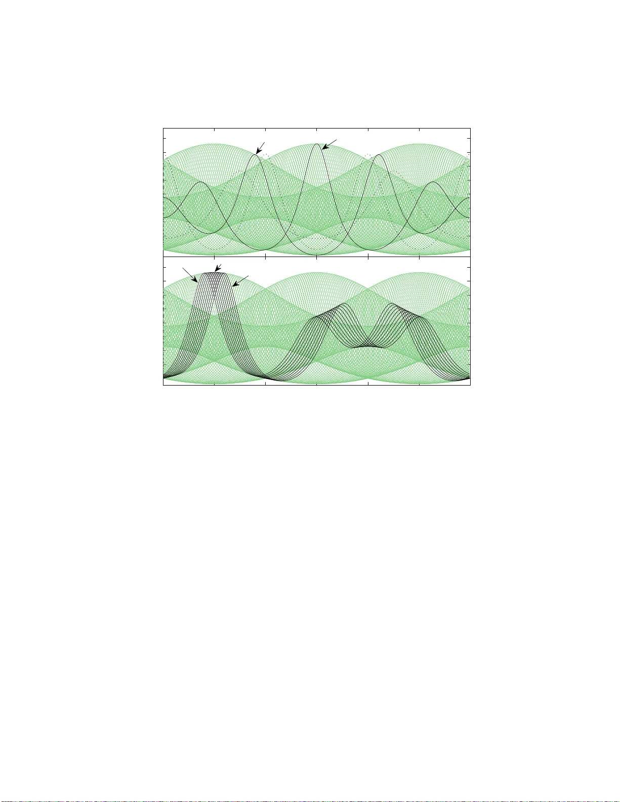
Global P aths of Time-P erio dic Solutions of the Benjamin-Ono Equation Connecting P airs of T ra v eling W a ves Da vid M. Am brose ∗ Jon Wilk ening † August 12, 2018 Abstract W e classify all bifu r cations from trav eling wav es to non-trivial time-p erio dic solutions of the Benjamin-Ono equation that are predicted b y linear iz ation. W e use a spectra lly accurate n umerica l contin uation method to study several paths of no n-trivial solutio ns beyond the rea lm of linear theory . These paths are found to either re- connect with a diﬀerent traveling w ave or to blow up. In the latter case , a s the bifurcation par ameter approaches a critical v alue, the amplitude of the initia l condition g ro ws without b ound and the per iod appr oac hes zero. W e then pr o ve a theo r em that gives the mapping from one bifurcation to its counterpart on the other side of the path and ex hibits exact formulas for the time-p erio dic s olutions o n this path. The F ourier co eﬃcients of these solutions are p o wer sums of a ﬁnite num b er of particle p ositions whose elementary symmetric functions execute simple orbits (circles or epicycles) in the unit disk of the complex plane. W e also ﬁnd exa mples of interior bifurc a tions from these paths of alrea dy non-trivial solutions, but we do not attempt to analy z e their ana lytic structure. Key w ords. P erio dic solutions, Benjamin-Ono equation, non-linear wa v es, solitons, bifurcation, con tin uation, exact solution, adjoin t equation, sp ec tral metho d AMS sub ject classiﬁcations. 65K10, 37M20, 35Q53, 37G15 1 In tro duction The Benjamin-Ono equation is a non-lo cal, n on -linear disp ersiv e equation in tend ed to de- scrib e the propagation of in tern a l wa v es in a d e ep , stratiﬁed ﬂuid [6 , 15, 30 ]. In spite of non-lo cal ity , it is an integ r ab le Hamil tonian system with meromorph ic particle solutions [12, 13], N -soliton solutions [24], an d N -phase multi-perio dic solutions [32, 16, 26]. A bilin- ear formalism [32] and a B¨ ac klund transf orm a tion [28, 7, 25] hav e b een found to generate sp ecial solutions of the equation, and, in the non-p erio dic setting of rapidly deca yin g initial ∗ Department of Mathematics, Drexel Un iversit y , Philadelphia, P A 19104 ( ambrose@math.drexe l.edu ). This w ork was supp orted in p a rt by the National Science F oundation th rou gh grant DMS-0926378. † Department of Mathematics and Lawrence Berkeley National Lab oratory , Universit y of California, Berke ley , CA 94720 ( wi lken@math.berkeley .edu ). This work was supp orted in part by the Director, Of- ﬁce of Science, Co mp utational and T echnolo gy Research, U.S. Department of Energy und er Contract No. DE-AC02-05 CH11231. conditions, an in verse scattering transform has b een dev elop ed [18, 20] that exploits an in- teresting Lax pair s tructure in wh ic h the solution pla ys the role of a compatibilit y condition in a Riemann-Hilb ert p roblem. It is common practice in numerical an alysis to test a numerical metho d u sing a problem for whic h exact solutions can b e found. O ur initia l in terest in Benjamin-Ono wa s to serv e as su c h a test problem. Although man y of the to ols mentio n e d ab o v e can b e used to study time-p eriodic solutions, th e y do not generalize to p roblems s uc h as the vorte x sh e et w it h surface tension [2, 4] or the true wa ter w a ve [31, 19], which are not known to b e in tegrable. Our goal in this p aper is to deve lop tools t h a t wil l generalize to these hard er problems and use them to study bifur ca tion and global reconnection in the s p ac e of time-p eriodic solutions of B-O. Sp eciﬁcally , we emp lo y a v ariant of the n u merica l contin uation metho d w e in tro duced in [3] for this pu rp ose , whic h yields solutions that are accurate enough that w e are able to recognize their analytic form. Because w e approac hed the problem f rom a completely diﬀeren t viewp oin t, our de- scription of these exact solutions is v ery diﬀerent fr om previously k n o wn represen tations of m ulti-p erio dic solutions. Rather than solv e a system of non-linear algebraic equations at eac h x to ﬁnd u ( x, t ) as was done in [26 ], we represent u ( x, t ) in terms of its F ourier co e ﬃ c ients c k ( t ), whic h turn out to b e p o w er s ums c k = 2[ β k 1 + · · · + β k N ] of a collection of N particles β j ( t ) evolvi n g in the unit disk of the complex plane as the zeros of a p olyno- mial z 7→ P ( z , t ) wh o se co eﬃci ents execute simple orbits (circles or epicycles in C ) . The connection b et ween the new representati on and previous r epresen tations w il l b e explored elsewhere [37]. Man y of our ﬁnd ings on the structure of bifu rcat ions and reco n necti ons in the manifold of time-p erio dic solutions of the Benjamin-On o equation are likely to hold for other systems as w ell. One inte r est in g p it f a ll we ha ve iden tiﬁed b y applying our m e th od to an inte grable problem is that degenerate b ifurcations can exist that are not predicted b y coun ting linearly indep endent , p erio d ic solutions of the linearization ab out trav eling w a ves. Although it is p ossible that such degeneracy is a consequence of the symmetries that make this p roblem in tegrable, it is also p ossible that other problems su c h as th e w ater w a ve will also p ossess degenerate bifurcations that are in visible to a linearized analysis. W e ha v e also found th a t one cannot ac hiev e a complete u nderstanding of these manifolds of ti m e-p erio dic solutions b y holding e.g. the mean constant and v arying only one parameter. I n some of the sim ulations where we hold the mean ﬁxed, the solution (i.e. the L 2 norm of the initial condition) blows up as the parameter approac hes a critical v alue rather than reconnecting with another tra veling w av e. Ho w ever, if the mean is sim u lt aneously v aried, it is alw ays p ossible to reconnect. Th u s, although n u merica l con tinuat ion with m o r e than one p a r ame ter is diﬃcult, it will lik ely b e necessary to explore m u lti -d im en sio n al parameter sp a ces to ac h ie ve a thorough understand ing of time-p eriodic solutions of other problems. On the numerical s id e, we b eliev e our use of certain F ourier mo des of the initial condi- tions as bifu rcati on parameters will pr o v e useful in many other problems b ey ond Benjamin- Ono. W e also wish to advocate the use of v ariatio n a l calculus and optimal con trol for the purp ose of ﬁnd in g time-perio dic solutions (or solving other t wo p oin t b oun dary v alue problems). F or ODE, a comp eting metho d kn o wn as orthogonal collo cat ion (e.g. as imp le - men ted in A UTO [17]) has pro ve d to b e a ve r y p ow erful tec h nique for solving b oundary v alue problems. This app r oa ch b ecomes quite exp ensiv e when the dimension of the system 2 increases, and is therefore less comp etitiv e for PDE than it is f or ODE. F or PDE, man y authors do not att emp t to ﬁ nd exact p erio dic solutions, and instead p oin t out that typical solutions of certain equations do tend to pass near their initial states at a later time [11]. If true p eriod ic solutions are sought, a m o r e common approac h has b een to either iterate on a P oincar ´ e map and use stabilit y of the orbit to ﬁnd time-p erio dic solutions [10], or u se a shooting metho d [33, 34] to ﬁnd a ﬁxed p oin t of the P oincar ´ e map. In a s h ooting method, w e deﬁn e a f u nctio n al F ( u 0 , T ) = [ u ( · , T ) − u 0 ] that m a p s initial conditions and a su pp osed p eriod to the deviation from p erio dicit y . The equation F = 0 is then solv ed b y Newton’s metho d, where the J a cobian J = D F is either co mp uted u sing ﬁnite d iﬀeren ces [35] or b y s o lvin g the v ariational equ ation rep eatedly to compu te eac h column of J . W e ha ve foun d that it is muc h more eﬃcien t (b y a f actor of the num b er of columns of J ) to instead minimize th e scalar functional G = 1 2 k F k 2 via a quasi-Newton metho d in whic h the gradien t DG is computed by solving an adjoin t PDE. Bristeau et . al. [8] dev elop ed a similar a p proac h for linear (bu t tw o- or three-dimensional) scattering p roblems. Thr ee dimensional problems are in tractable b y the standard sho oting approac h as J could easily ha ve 10 5 columns. How ev er, the gradient of G ca n b e compu te d b y solving a single adjoin t PDE. The success of the method then b oils do wn to a question of the num b er of iterat ions required for the minimization algorithm to conv erge. F or linear problems, Bristeau et. al. hav e had success u sing conjugate gradien ts to minimize G . W e ﬁnd that BFGS [9 ] works v ery w ell for nonlin ear problems lik e th e Benjamin-On o equation and the v ortex sh e et with surface tension [4]. T o ﬁnd non-trivial t ime-p erio dic solutio n s in the pr ese nt w ork, we use a sym m et r ic v arian t of the algorithm describ ed in [3]. Although the origi n al metho d works w ell, w e use the symmetric v ariant for the simulatio n s in this pap er b ecause evo lvin g to T / 2 requires half the time-steps and yields more acc u rate answ ers (as there is less time for n um er ical roundoﬀ error to corrupt the calculat ion). Moreo v er, the n umb er of degrees of f r ee d om in the searc h s p ac e of initial conditions is also cut in half and the condition num b er of the problem improv es when we eliminate phase shift degrees of freedom via symmetry r a th er than including them in the p enalt y function describ ed in Sectio n 3.1. Although w e do not mak e use of it, there is a p r ocedure kno wn as the Mey er-Marsden-W einstein reduction [27, 23] that allo ws one to reduce the dimension of a sym plect ic manifold on whic h a group acts symplectically . This allo ws one to eliminate actions of the group (e.g. trans la tions) from the phase space. Equilibr ia and p eriod ic solutions of the redu ce d Hamiltonian s yste m corresp ond to (familie s of ) relativ e equilibria and relativ e p erio dic solutio n s [39] of the original system. This pap er is organized as follo ws . In S e ction 2, we discuss stationary , tra ve ling and par- ticle solutions of B-O, linearize ab out tra v eling wa v es, and classify all bifurcations predicted b y linear theory f rom tra ve ling wa v es to non-trivial time-p eriod ic solutions. Some of the more tec h nical material from this section is giv en in App endix A. In S ection 3, w e presen t a collect ion of numerical exp eriments usin g our contin uation metho d to follo w s e veral paths of non-trivial solutions b ey ond the realm of linear theory in ord er to formulate a theorem that gives the global mapping fr o m one tra vel in g wa v e b if u rcati on to its coun terpart on the other side of the path. In Section 4, we stud y the b eha vior of the F ourier mo des of the time-p erio dic solutions found in Section 3 and state a theorem ab out the exact form of these solutions, w hic h is prov ed in App endix B. Finally , in Section 5, w e discuss inte - 3 rior bifurcations from these paths of already non-trivial solutions to still more co m plica ted solutions. Although the existence of such a hierarc h y of solutions was alrea d y kno wn [32], bifurcation b e tw een v arious lev els of the hierarc h y has not previously b een discuss e d . 2 Bifurcation from T ra v eling W a v es In this section, we study the linearizat ion of the Benjamin-On o equation ab out stationary solutions and tra v eling w a ves by so lvin g an inﬁ n ite d imensional eigenv alue problem in closed form. Eac h eigen ve ctor corresp onds to a time-p erio dic solution of the linearized equation. The tr a veling case is red u ce d to the stationary case by requiring th a t th e p erio d of the p erturbation (with a suitable spatial ph ase sh ift) coincide with the p erio d of the tr av eling w av e. The main goal of this section is to devise a classiﬁcation scheme of the bifur ca tions from tra vel in g w a ves s o that in later sections we can describ e w h ic h (local) bifurcations are connected tog ether by a global path of non-trivial time-per io dic solutio n s. 2.1 Stationary , T ra v eling and P article Solutions W e consider the Benjamin-Ono equatio n on the p eriodic in terv al R  2 π Z , n ame ly u t = H u xx − uu x . (1) Here H is the Hilb ert transform, w hic h has th e sy mb ol ˆ H ( k ) = − i sgn( k ) . T h e Benj amin - Ono equatio n p ossesses solutions [12, 3] of the form u ( x, t ) = α 0 + N X l =1 φ ( x ; β l ( t )) , (2) where α 0 is the mean, β 1 ( t ), . . . , β N ( t ) are the tra jectories of N particles ev olving in th e unit disk ∆ of the complex plane and go v ern e d b y the ODE ˙ β l = N X m =1 m 6 = l − 2 iβ 2 l β l − β m + N X m =1 2 iβ 2 l β l − ¯ β − 1 m + i (2 N − 1 − α 0 ) β l , (1 ≤ l ≤ N ) , (3) and φ ( x ; β ) is the function with F ourier representa tion ˆ φ ( k ; β ) =    0 , k = 0 2 β k , k > 0 2 ¯ β | k | , k < 0    , β ∈ ∆ = { z : | z | < 1 } . (4) The function φ ( x ; β ) has a p eak cente r ed at x = arg ( ¯ β ) with amplitude gro wing to in ﬁnit y as | β | appr oac h es 1. The N -h ump tra v eling wa v es (with a spatial p eriod of 2 π / N ) are a sp ecial case of th e particle solutions given by (2) and (3) : u tra v ( x, t ; α 0 , N , β ) = α 0 + N X l =1 φ ( x ; β l ( t )) , β l ( t ) = N p β e − ict , c = α 0 − N α ( β ) . ( 5) 4 Eac h β l is assigned a distinct N t h ro ot of β and α ( β ) is the mean o f th e one-hump stat ionary solution, namely α ( β ) = 1 − 3 | β | 2 1 − | β | 2 , | β | 2 = 1 − α ( β ) 3 − α ( β ) . (6) The solution (5) mo v es to the righ t when c > 0. Indeed, it ma y also b e w ritte n u tra v ( x, t ; α 0 , N , β ) = u stat ( x − ct ; N , β ) + c, (7) where u stat is the N -h u mp stationary solution u stat ( x ; N , β ) = N α ( β ) + X { γ : γ N = β } φ ( x ; γ ) = N α ( β ) + N φ ( N x ; β ) . (8) The F our ie r rep resen tation of u stat is ˆ u stat ( k ; N , β ) =            N α ( β ) , k = 0 , 2 N β k / N , k ∈ N Z , k > 0 , 2 N ¯ β | k | / N , k ∈ N Z , k < 0 , 0 otherwise. (9) Amic k and T oland hav e shown [5] that all trav eling wa v es of the Benjamin-Ono equation ha ve the form (7); see also [37]. 2.2 Linearization ab out Stationary Solutions Let u ( x ) = u stat ( x ; N , β ) b e an N -h ump stationary solution. In [3], we solved th e lineariza- tion of (1) ab out u , namely v t = H v xx − ( uv ) x = iB Av , A = H ∂ x − u, B = 1 i ∂ x , (10) b y substituting v ( x, t ) = Re { C z ( x ) e iω t } in to (10) and solving the eigen v alue problem B Az = ω z (11) in clo sed form. S p eciﬁcally , w e sho wed that the eig env alues ω N ,n are giv en b y ω N ,n =        − ω N , − n , n < 0 0 n = 0 ( n )( N − n ) , 1 ≤ n ≤ N − 1 ( n + 1 − N )  n + 1 + N (1 − α ( β ))  , n ≥ N        0 30 0 500 N=20, β =1/2 n ω N,n (12) The zero eigen v alue ω N , 0 = 0 has ge ometric m ultiplicit y t wo and algebraic m u lti p lic ity three. The eigenfunctions in the k ernel of B A are z (1 , 0) N , 0 ( x ) = − ∂ ∂ x u stat ( x ; N , β ) , z (2) N , 0 ( x ) = ∂ ∂ | β | u stat ( x ; N , β ) , (13) 5 whic h c orr espond to c h anging the p hase or amplitude of β in the underlying stationary solution. There is also a Jordan chain [36] of length t wo associated with z (1 , 0) N , 0 ( x ), namely z (1 , 1) N , 0 ( x ) = 1 ,  iB Az (1 , 1) N , 0 = z (1 , 0) N , 0  , (14) whic h corresp onds to the fact that add ing a constan t to a stationary solution causes it to tra v el. The fact that all the eigen v alues iω N ,n in the linearization (10 ) are purely imaginary is a consequence of the Hamiltonian structure [13] of the Benjamin-Ono equation. F or non- Hamiltonian systems, one do es not generally exp ect to ﬁnd time-perio dic p erturbations of tra v eling w av es (as p erio dic solutions of the linearized problem may not ev en exist). The eigenfunctions z N ,n ( x ) corresp onding to p ositiv e eigen v alues ω N ,n (with n ≥ 1) ha ve the F o u rier representa tion ˆ z N ,n ( k )    k = n + j N =     1 + N ( | j |− 1) N − n  ¯ β | j |− 1 j < 0 C  1 + N j n  β j +1 j ≥ 0    , 1 ≤ n ≤ N − 1 C = − nN ( N − n )  n +( N − n ) | β | 2  ! , ˆ z N ,n ( k )    k = n +1 − N + j N =          0 j < 0 − ¯ β (1 −| β | 2 ) 2 h 1 −  1 − N n +1  | β | 2 i j = 0  1 + N ( j − 1) n +1  β j − 1 j > 0          , ( n ≥ N ) , (15) with all other F ourier co eﬃcien ts equal to zero. Th e eigenfun c tions corresp onding to nega- tiv e eigen v alues ω N ,n (with n ≤ − 1) satisfy z N ,n ( x ) = z N , − n ( x ), so the F ourier coeﬃcients app ear in rev erse ord er, conjugated. F or 1 ≤ n ≤ N − 1, an y linear com bin a tion of z N ,n ( x ) and z N ,N − n ( x ) is also an eigenfunction; how ev er, the c h oices here seem m o s t natural as they sim u lta n eously diagonalize the s hift op e r at or (discussed b elo w) and yield directions along whic h non-trivial solutions exist b ey ond the linearization. S a id diﬀeren tly , w e ha v e listed the ﬁrst N − 1 p ositiv e eigenv alues ω N ,n in an un u sual order (rather than en umerat- ing them monotonically and coalescing m u lti p le eigen v alues) b ecause this is the order that leads to the simplest description of the global paths of non-trivial solutions connecting these tra v eling w av es. 2.3 Classiﬁcation of bifurcations from trav eling wa v es Time-p eriod ic solutio n s of the Benjamin-On o equation with p eriod T ha v e initial conditions that satisfy F ( u 0 , T ) = 0, where F : H 1 × R → H 1 is giv en b y F ( u 0 , T ) = u ( · , T ) − u 0 , u t = H u xx − uu x , u ( · , 0) = u 0 . (16) W e b egin by linearizing F ab out an N -hump stationary soution u 0 ( x ) = u stat ( x ; N , β ). The F r ´ ec het deriv ativ e D F = ( D 1 F , D 2 F ) : H 1 × R → H 1 yields d irect ional deriv ativ es D 1 F ( u 0 , T ) v 0 = ∂ ∂ ε    ε =0 F ( u 0 + εv 0 , T ) = v ( · , T ) − v 0 =  e iB AT − I  v 0 , D 2 F ( u 0 , T ) τ = ∂ ∂ ε    ε =0 F ( u 0 , T + ετ ) = 0 . (17) 6 Note that v 0 ∈ k er D 1 F ( u, T ) if and only if the solution v ( x, t ) of the linearized problem is p eriod ic with p erio d T . As a result, a b a s is for the kernel N = k er D F ( u 0 , T ) consists of (0; 1) toge ther with all pairs ( v 0 ; 0) of the form v 0 ( x ) = Re { z N ,n ( x ) } or v 0 ( x ) = Im { z N ,n ( x ) } , (18) where n ranges o v er all in tegers such that ω N ,n T ∈ 2 π Z (19) with N and β (in the form ula (12) for ω N ,n ) held ﬁ xed. The co r r espond ing p erio dic solutions of the linearized problem are v ( x, t ) = Re { z N ,n ( x ) e iω N,n t } or v ( x, t ) = Im { z N ,n ( x ) e iω N,n t } . (20) Negativ e v alues of n ha ve already b een accoun ted for in (18) and (20) using z N , − n ( x ) = z N ,n ( x ), and the n = 0 case alw a ys yields t wo ve ctors in the ke r nel, namely those in (13). These directio n s do not cause bifu rcat ions as they lead to other stationary solutions. Next w e wish to linearize F ab out an arb it r a r y tra vel in g wa v e. Supp ose u ( x ) = u stat ( x ; N , β ) is an N -h um p stationary solutio n and U ( x, t ) = u ( x − ct ) + c is a tra v el- ing w a ve. Then the solutions v and V of the linearizatio n s ab out u and U , resp ectiv ely , satisfy V ( x, t ) = v ( x − ct, t ). Note also that F ( U 0 , T ) = 0 iﬀ cT = 2 π ν N for some ν ∈ Z , (21) where U 0 ( x ) = U ( x, 0) = u ( x ) + c . Note that ν is the num b er of times the tra ve ling wa v e turns o v er itself in one p erio d. Assuming (21) holds, we set θ = 2 π ν / N and compute [ D 1 F ( U 0 , T ) v 0 ]( x ) = v ( x − cT , T ) − v 0 ( x ) = [( S θ e iB AT − I ) v 0 ]( x ) , [ D 2 F ( U 0 , T ) τ ]( x ) = U t ( x, T ) τ = − cu x ( x − cT ) τ = − cu x ( x ) τ , (22) where v solv es (10) and the shift op er ator S θ is deﬁned via S θ z ( x ) = z ( x − θ ) , ˆ S θ , kl = e − ik θ δ k l . (23) One ele m e nt of N = k er D F ( U 0 , T ) arises from (14 ), whic h giv es e iB At 1 = 1 − tu x ⇒ D 1 F ( U 0 , T )( − c/T ) + D 2 F ( U 0 , T )1 = 0 , and imp lie s ( − c/T ; 1) ∈ N . Th is just means that we can c hange the p eriod T b y a small amoun t τ b y add ing th e constan t − ( c/T ) τ to U 0 ; (this also follo ws from the condition (21 ) that cT = θ = const). If we wish to c hange the p erio d w ith ou t c hanging the mean, w e need to sim ultaneously adjust | β | in the u nderlying sta tionary solution u ( x ) = u stat ( x ; N , β ). The other elemen ts of N are of the form ( v 0 ; 0) with v 0 ( x ) = Re { z N ,n ( x ) } or v 0 ( x ) = Im { z N ,n ( x ) } . (24) The admissible v alues of n here are found using (22 ) together with S θ e iB AT z N ,n = e i ( ω N,n T − θ k N,n ) z N ,n , θ = 2 π ν N , (25) 7 where k N ,n is the stride oﬀset of the non-zero F ourier co eﬃcien ts of z N ,n , i.e. ˆ z N ,n ( k ) 6 = 0 ⇒ k − k N ,n ∈ N Z . (26) Th u s, instead of (19), n ranges o ve r all intege r s suc h that ω N ,n T ∈ 2 π  ν k N ,n N + Z  , k N ,n =            − k N , − n , n < 0 , 0 n = 0 , n 1 ≤ n ≤ N − 1 , mo d( n + 1 , N ) n ≥ N . (27) As b efore, n eg ativ e v alues of n need not b e considered once we tak e r ea l and imaginary parts in (24), and the n = 0 case alwa ys gives the tw o vecto r s ( z (1 , 0) N , 0 ; 0) , ( z (2) N , 0 ; 0) ∈ N , whic h lead to other tra ve lin g wa v es rather than bifurcations to non-trivial solutions. Our numerical exp erimen ts ha ve led us to the follo wing conjecture, which w e prov e as part of Theorem 3 in Section 4: Conjecture 1 F or ev e ry β ∈ ∆ and ( N , ν, n, m ) ∈ Z 4 satisfying N ≥ 1 , ν ∈ Z , n ≥ 1 , m ≥ 1 , m ∈ ν k N ,n + N Z , (28) ther e is a four p ar ameter she et of non-trivial time-p erio dic solutions bifu r c ating fr om the N - hump tr aveling wave with sp e e d index ν , ( cT = 2 π ν / N ), bifur c ation index n , and oscil lation index m , ( ω N ,n T = 2 π m/ N ). The phase and amplitude of the tr aveling wave ar e determine d by β . The main con ten t of this conjecture is that we d o not ha ve to consider linear com b i- nations of the z N ,n with diﬀerent v alues of n to ﬁn d p erio dic s olutions of the non-linear problem — this basis is already “diagonal” with resp ect to these bifurcations. This is true in spite of a sm a ll divisor problem prev enting DF ( U 0 , T ) from b eing F redholm. The decision to num b er the ﬁrst N − 1 eigenv alues ω N ,n non-monotonically in (12) and to simulta n eo u s ly diagonalize the shift op erator S θ when c ho osing eigen v ectors z N ,n in (15 ) w as essenti al to mak e th is work. F orm ulas relating the p erio d, T , the mean, α 0 , and the deca y p arame ter, | β | , for eac h of these bifurcations are giv en in App endix A along with a list of bifurcation rules go v erning “legal” v alues of the m ean. A canonica l wa y to generate one of these b ifurcations is to take β real an d p erturb the initial condition in the direction v 0 ( x ) = Re { z N ,n ( x ) } . This leads to non-trivial solutions with ev en symmetry at t = 0. Perturbation in the Im { z N ,n ( x ) } direction yields the s a m e set of non-trivial solutions, but with a s p at ial and temp oral phase shift: Im { z N ,n ( x − ct ) e iω t } = Re n z N ,n  x − cπ 2 ω  − c  t − π 2 ω  e iω ( t − π 2 ω ) o , (29) where ω = ω N ,n . Th e man if old of non-trivial solutions is fou r dimen s io n a l with t wo essen tial parameters (e.g. the m ea n α 0 and a parameter go verning th e distance fr o m the tra v eling w av e) and t wo inessentia l parameters (the sp at ial and temp oral phase). In our numerical studies, w e use the real p a r t of a F ourier co e ﬃ c ient c k of the initial condition (with k s uc h 8 that ˆ z N ,n ( k ) 6 = 0) for the second essen tial bifurcation p arameter. Wh en we d iscuss exact solutions in Section 4, a diﬀerent parameter will b e used. W e remark that this enumeration of b ifurcatio n s accoun ts for all time-p erio d ic solutions of t h e linearization a b out tra v eling wa ves; therefore, the heuristic t h at eac h bifurcation of the non-linear problem g ives r ise to a linearly indep endent v ector in the k ern el N of the linearized problem suggests th at w e ha v e found all bifurcations from trav eling w a ves. In terestingly , th is turns out n ot to b e the case ; the interior bifur ca tions w e d iscuss in Section 5 ca n o ccur at th e en d p oints of the path, allo wing for degenerate bifurcations directly from trav eling w a v es to higher lev els in th e in ﬁnite h ierarch y o f time-p eriodic solutions. Only the transition from the ﬁrst level of the h ierarc h y to the second is “visible” to a linearize d analysis ab out tra veling wa v es. Th e other transitions b ecome linearly dep endent on these in the limit as the tra veli n g wa v e is approac hed; they will b e analyzed in [37]. 3 Numerical Exp erimen ts In this sectio n we present a colle ction of n um eric al exp erimen ts in w hic h w e start with a giv en bifurcation ( N , ν, n , m, β ) and use a symmetric v ariant of th e metho d we describ ed in [3] for ﬁnding perio dic solutions of non-linear PDE to conti nue these solutions until another trav eling w a ve is found, or until the solution blo w s up as the bifurcation parameter approac hes a critical v alue. W e d etermin e the bifur ca tion indices ( N ′ , ν ′ , n ′ , m ′ ) at the other end of th e p a th of non-trivial solutions b y ﬁtting the d a ta to the formulas of the pr evio u s section. By trial and err o r , w e are then able to guess a formula relating ( N ′ , ν ′ , n ′ , m ′ ) to ( N , ν , n, m ) that we use in S ec tion 4 to constru c t exact solutions. 3.1 Numerical Metho d As mentioned in S ection 2.3, a natur a l c h oi ce of spatial and temp oral phase can b e ac hiev ed b y c h oosing th e p aramet er β o f t h e tra vel in g wa v e to b e real and p erturbing th e initial condition in the directio n v 0 ( x ) = Re { z N ,n ( x ) } . F or reasons of e ﬃ c iency and ac cu r ac y (explained in the in tro duction), we no w r e s tric t our searc h for time-p erio dic solutions of (1) to functions u ( x, t ) that p ossess even sp at ial symmetry at t = 0. If we succeed in ﬁn ding solutions with th is symmetry , then they (together with t h ei r phase-shifted co u n terparts analogous to (29)) s p an the nullspace N = ker D F ( U 0 , T ) in the limit that the p ertur b at ion go es to zero. Thus, w e d o not exp ect symmetry breaking bifurcations fr o m tr a veling wa v es that cannot b e phase shifted to h a v e ev en symmetry at t = 0. The Benjamin-Ono equation has the prop ert y th at if u ( x, t ) is a solution of (1), then so is U ( x, t ) = u ( − x, − t ). As a resu lt, if u is a solution suc h that u ( x, T / 2) = U ( x, − T / 2), then u ( x, T ) = U ( x, 0), i.e. u is time-p e r iodic if the initial condition has even symmetry . Th u s, w e seek initial conditions u 0 with ev en symmetry and a p eriod T to minimize the functional G tot ( u 0 , T ) = G ( u 0 , T ) + G penalty ( u 0 , T ) , (30) where G ( u 0 , T ) = 1 2 Z 2 π 0 [ u ( x, T / 2) − u (2 π − x, T / 2)] 2 dx (31) 9 and G penalty ( u 0 , T ) is a non-negativ e p enalt y fun ct ion to imp ose the mean and set the bifurcation parameter. T o compute the gradien t of G with resp ect to v ariation of the initial conditions, w e use d dε     ε =0 G ( u 0 + εv 0 , T ) = Z 2 π 0 δ G δ u 0 ( x ) v 0 ( x ) dx, (32) where the v ariational deriv ativ e δ G δ u 0 ( x ) = 2 w ( x, T / 2) , w 0 ( x ) = u ( x, T / 2) − u (2 π − x, T / 2) (33) is f ou n d b y solving the follo win g adjoint equation from s = 0 to s = T / 2: w s ( x, s ) = − H w xx ( x, s ) + u ( x, T 2 − s ) w x ( x, s ) , w ( · , 0) = w 0 . (34) Since v 0 is assumed symmetric in this formulatio n , (33) is equiv alen t to δ G δ u 0 ( x ) = w ( x, T / 2) + w (2 π − x, T / 2) . (35) The Benjamin-Ono and adjoint equations are solv ed usin g a p seudo-sp e ctral collo cat ion metho d emplo ying a fourth order semi-implicit additive Run g e-Ku tt a metho d [14 , 21, 38] to adv ance the solution in time. Th e BF GS metho d [9, 29] is then used to min imiz e G tot (v ary in g th e p erio d and the F ourier co eﬃcien ts of the initial conditions). W e use the p enalt y function G penalty ( u 0 , T ) = 1 2  [ a 0 (0) − α 0 ] 2 + [ a K (0) − ρ ] 2  (36) to sp ecify t h e mean α 0 and th e real part ρ of the K th F o u rier co eﬃcien t of the initi al condition u 0 ( x ) = M / 2 X k = − M/ 2+1 c k (0) e ik x , c k ( t ) = a k ( t ) + ib k ( t ) . (37) The parameters α 0 and ρ serve as the bifurcation parameters while the phases are deter- mined by requiring that the s olution ha ve ev en symmetry at t = 0. W e generally c ho ose K to be the ﬁ rst k ≥ 1 suc h that ˆ z N ,n ( k ) 6 = 0. Our contin uation metho d consists of three stages. First, we c ho ose a tra ve ling w a v e and a set of bifurcation indices to b egin the path of non-trivial solutions. W e also choose a direction in whic h to v ary th e bif u rcati on parameter ρ and the m ean α 0 . I n most o f our n u merica l exp erimen ts, we hold α 0 ﬁxed; ho wev er, in the example of Figure 6 b elo w , w e v ary ρ and α 0 sim ultaneously . T h e tra v eling w a v e serv es as the zeroth p oin t on the path. The initial gu ess for the ﬁ rst p oint on the path is obtained b y p erturbing the in it ial condition of the tra ve lin g wa ve in the direction Re { z N ,n ( x ) } . W e u s e the p erio d T giv en in (77) in App endix A as a starting guess. W e then use the minimization algorithm to d esc en d from the starting guess predicted b y linear theory to an ac tual time-p eriod ic solution. Th e second stage of the conti nuation algorithm consists of v arying ρ (and p ossibly α 0 ), using linear extrap olation for the starting guess (for u 0 and T ) of the next s o lu ti on, and then minimizing G tot to ﬁn d an actual time-p eriodic solution w ith these v alues of ρ and α 0 . If the initial v alue of G tot from the extrap ol ation step is to o large, w e discard the step and 10 try again with a smaller change in ρ and α 0 . T he ﬁnal stage of the algorithm consists of iden tifying the reconnection o n the other side of the path. W e d o this b y b li n dly o vershooting the target v alues of ρ and α 0 (whic h we do not kno w in adv ance). Inv ariably , the algorithm will lo c k on to a family of tra ve ling wa v es once w e r e ach the en d of the path of non-trivial solutions. W e lo ok a t the F ourier coeﬃcients of the last non-trivial solution b efore the tra v eling wa ves are reac hed and matc h them with the formulas for ˆ z N ′ ,n ′ ( k ) to determine the correct bifur ca tion indices on this side of the path. (A p rime indicates ind ic es for the bifurcation at the other end of the path.) W e then recompute the last several s o lu ti ons on the path of n o n -t r ivia l solutions with app r opriate v alues of ρ and α 0 to arr iv e exactly at the tra veling w av e on the last iteration. W e sometimes change K in (36) to compute this reconnection to av oid ˆ z N ′ ,n ′ ( K ) = 0. The r unning time of our algorithm (on a 2.4 GHz d e s kto p mac hin e ) v aries from a few hours to compute one of the paths lab eled a – l in (38)–(41 ) b elo w, to a few d a ys to compute a path in which the solution blo ws up, such a s the one sho wn in Figure 5 b el ow. W e alw a ys reﬁne the mesh and timestep enough so that the sol u tio n s are essen tially exact (with G tot ≤ 10 − 26 in the easy cases an d 10 − 20 in the hard cases). 3.2 Global paths of non-trivial solutions W e no w inv estiga te the global b eha vior of non-trivial solutions that b if u rcate from arbi- trary stationary or tra veling wa v es. W e ﬁnd that these non-trivial solutions act as rungs in a ladd er , connecting stationary and tra veli n g solutions with d iﬀe r en t sp eeds and w av e- lengths by creating or ann ihila ting oscillatory humps th at grow or shrink in amplitud e u n til they b ecome part of the stationary o r tra v eling w a v e on th e other side of th e rung. In some cases, r a th er than re-connecting with an other tra v eling w av e, the solution blo ws up (i.e. the L 2 -norm of the initial condition gro ws without b ound) as the bifurcation parameter ρ app roa ches a critical v alue. Ho we ver, eve n in these cases a r e-connection with another tra v eling w a ve d oes o ccur if, in addition to ρ , w e v ary the m ean, α 0 , in an appropriate wa y . Recall f r om S ec tion 2.3 that w e can en umerate all such b ifurcations b y sp eci f y in g a complex parameter β in the unit disk ∆ along with four int egers ( N , ν, n, m ) satisfying (28), and in most cases we can solv e for | β | in terms of the mean, α 0 , using (8 0 ) in App endix A. In [3], we p resen ted a detailed stud y of the solutions on the path connecting a one-hump stationary solution to a tw o-h ump trav eling w av e mo ving left. W e denote this path by a : (1 , 0 , 1 , 1) ← → (2 , − 1 , 1 , 1) , (38) where th e lab el a refers to the bifurcation diagram in Figure 1. W e h a v e also computed the next several bifu r ca tions ( n = 2 , 3 , 4) from the one-h um p stationary solution and found that they connect up with a tra ve lin g w a ve with N ′ = n + 1 humps mo ving left with sp eed index ν ′ = − 1, where we denote the bifurcation on the other side of the path b y ( N ′ , ν ′ , n ′ , m ′ ). By comparing the F ourier co eﬃcients of the last few non-trivial solutions on these p a th s to those of the linearization ab out the N ′ -h um p trav eling wa v e, w e determined that the bifurcation and oscillati on indices satisfy n ′ = n and m ′ = 1, resp ectiv ely . S tu dying these reconnections rev ealed that the correct w ay to n um b er the eigen v alues ω N ′ ,n ′ w as to split the double eigen v alues with n ′ < N ′ apart as we did in (12) by simultaneously diagonalizing the shift op erator and ordering the ω N ′ ,n ′ via the stride oﬀset of the corresp ondin g eigen ve ctors 11 2.2 2.4 2.6 2.8 3 3.2 3.4 −1.5 −1 −0.5 0 0.5 1 1.5 First several bifurcations connecting stationary and traveling waves T a 2 (0) π 7d 8d 5c a 9d 3b 6c 10d 11d 7c 12d i f j e g k l h one−hump stationary, ±β two−hump traveling two−hump traveling constant and three−, four− and five−hump traveling P Figure 1: Pa th s of non-trivial solutions listed in equations (38)–(41). The second F ourier mo de of the eige nv ector z N ,n ( x ) in the linearization is non-zero for the pitc hfork bifu rcati ons and is zero for the one-sided, oblique-angle bifurcations. Th e p oint lab e led P corresp onds to the solution in Fig . 3 b elo w. (rather than monotonically). Using this orderin g , the non-trivial solutions connect u p with the N ′ -h um p tra ve ling w a ve along the z N ′ ,n ′ direction (without in volving z N ′ ,N ′ − n ′ ). T hese results are sum marize d as b : (1 , 0 , 2 , 1) ← → (3 , − 1 , 2 , 1) , c : (1 , 0 , 3 , 1) ← → (4 , − 1 , 3 , 1) , d : (1 , 0 , 4 , 1) ← → (5 , − 1 , 4 , 1) . (39) The lab els a , b , c , d in (38) and (39) corresp ond to the paths lab eled 7 d , 8 d , 5 c , a , etc. in the bifurcation diagram. When an in teger p pr ec edes a lab el, it m e ans that the p eriod T that is plotted is p times larger than the f u ndamen tal p erio d of the solution r epresen ted. Thus, curv e 7 d is the image of cur v e d (n ot shown) under the linear tran s formati on ( T , a 2 ) 7→ (7 T , a 2 ). In our lab eling sc heme, w e just n ee d to m u lti p ly ν , m , ν ′ , m ′ b y p to obtain the new path, e.g. 7 d : (1 , 0 , 4 , 7) ← → (5 , − 7 , 4 , 7) . (40) In this diagram, we p lot a 2 (0) vs. T w ith the spatial and temp oral phases chosen so the solution is ev en at t = 0. F or example, on path d , as w e decrease ρ = a 2 (0) from 0 . 3710 87 to 0, the solution transitions fr o m the one-hump statio n ary solution to the ﬁve -hump left- tra v eling w av e as sho w n in Figure 2. 12 0 π/3 2π/3 π 4π/3 5π/3 2π −3 −1.5 0 1.5 3 4.5 6 Periodic solution between one−hump stationary and five−hump traveling waves u x T = 0.288322 a 2 (0) = 0.366113 t = 0 t = T/2 stationary solution traveling wave (t = 0) Figure 2: Periodic solution on path d connecting the one-hump stationary solution to the ﬁv e-hump left-tra veling wa v e ( α 0 = 0 . 54437 5). The seco n d F ourier mo de of z 1 , 4 ( x ) is zero, whic h explains why a 2 (0) = 0 . 366113 for this solution is only 1 . 35% of the w a y b et w een the stationary solution a 2 (0) = 0 . 371087 and the ﬁve-h ump tra v eling wa v e a 2 (0) = 0. It is in teresting that the paths lab eled a and 3 b in Figure 1 meet the one-hump sta tionary solutions in a pitc h f o r k while the other paths (suc h as 5 c and 8 d ) meet at an oblique angle from one side only . This is b ecause the second F ourier mo de of the eigen v ector z 1 ,n ( x ) in the linearizatio n ab out the stationary solution is zero in these latter cases, s o the c hange in a 2 (0) from that of the stationary solution (namely 0 . 371087) is a higher order eﬀect, (a s is the c hange in T ). This explains the obliqu e angle. W e no w explain wh y these bifurcations o cc u r from one side only . When we go b ey ond the linearization as we ha ve here, we ﬁnd that c 2 ( t ) = a 2 ( t ) + ib 2 ( t ) has a nearly circular (epitro c hoidal) orbit in case a , a circular orb it in case b , and remains constan t in time in cases c and d (see Section 4). If one branc h of the pitc hfork corresp onds to a 2 (0), the other is a 2 ( T / 2) since the f unction u ( · , T / 2) also has ev en symmetry . But in ca s e s c and d , a 2 (0) is equal to a 2 ( T / 2) even though the functions u ( · , 0) and u ( · , T / 2) are diﬀerent . These cases also become pitc hforks when a diﬀeren t F ourier coeﬃcien t a K (0) is used as the bifurcation parameter. Next we compute the ﬁrst seve r a l bifurcations fr om the t wo -hump tra veling w a v es with mean α 0 = 0 . 544375 and sp eed index ν = − 1. W e set N = 2, ν = − 1, n ∈ { 1 , 2 , 3 , 4 } and choose the ﬁrst sev eral legal m v alues, i.e. v alues of m that satisfy the bifu rcat ion rules of Figure 14 in App endix A. F or example, the curves lab el ed i , j , k and l in Figur e 1 corresp ond to the b if u rcati ons (2 , − 1 , 4 , m ) w it h m = 11 , 13 , 15 , 17; smaller v alues (and ev en 13 v alues) of m are not allo w ed. In add ition to the p at h a in (38) ab o v e, w e obtain the p aths e : ( 2 , − 1 , 2 , 3) ← → (3 , − 3 , 1 , 3) , f : (2 , − 1 , 3 , 6) ← → (4 , − 5 , 2 , 6) , g : (2 , − 1 , 3 , 8) ← → (4 , − 6 , 2 , 8) , h : (2 , − 1 , 3 , 10) ← → (4 , − 7 , 2 , 10) , i : (2 , − 1 , 4 , 11) ← → (5 , − 8 , 3 , 11) , j : (2 , − 1 , 4 , 13) ← → (5 , − 9 , 3 , 13) , k : (2 , − 1 , 4 , 15) ← → (5 , − 10 , 3 , 15) , l : (2 , − 1 , 4 , 17) ← → (5 , − 11 , 3 , 17) . (41) The paths f , g and h meet the cur v e representi n g the t w o-hump tra veling w av es in a pitc hfork bifu r ca tion while th e others meet o b li q u ely fr om one side. Th is, again, is an anomaly of ha ving c h ose n the s econd F ourier mo de for the bifurcation parameter. Th e dotted line nea r the path e is th e curv e obtained when e is reﬂecte d across the T -axis. Solutions on t h is dotted lin e corresp ond to solutions on path e shifted b y π / 2 in sp ac e, whic h c hanges the sign of ρ = a 2 (0) bu t also breaks the ev en symmetry of the solution at t = 0. The p a th s lab eled i , j , k and l are exactly symm etric when reﬂected ab out the T -axis b ecause c 2 ( t ) has a circular orb it cent ered at zero in th ese cases. It is in teresting that so man y of the paths in this bifurcation diagram termin ate wh en T = π (or a simple ratio n a l m ultiple of π ). Th is is due to the fact that T in (77) in App end ix A is indep endent of α when n < N . The solutions u ( x, t ) corresp onding to p oin ts along the paths b , c and d are qualitativ ely similar to eac h other. As sh o wn in Fig u re 2, these solutions look lik e N ′ -h um p wa v es tra v- eling o v er a stationary one-h u mp carrier signal. A t one end of the p at h the high frequency w av e ma y b e view ed as a p erturbation of the one-h ump stationary solution, while at the other end of the path it is more app ropriate to regard the stationary s o lu ti on as th e p ertur- bation, causing the tra v eling wa ve to bulge upw ard as it p asses n ea r x = π an d d o wn ward near x = 0 and x = 2 π . In all these cases, the solution rep eats itself when one of the high frequency w a ves h as mo ve d left one slot to assume the shap e of its left n ei ghb or at t = 0. By con trast, the solutions that bifur c ate from the t wo -hump tra veli n g w a ves, i.e. those on the p at h s listed in (41), hav e the prop ert y that wh en a wa ve has m ov ed left one slot to the lo cati on that its neigh b or o ccupied at t = 0, it h as acquired a diﬀerent shap e and must k eep p r og r essin g a num b er of slots b efore it ﬁnally lines up with one of the initial w av es. This is illustrated in Fig u re 3 for the solution lab e led P in Figure 1 on the path e : (2 , − 1 , 2 , 3) ← → ( 3 , − 3 , 1 , 3) . (42) This solution is qualitat ively similar to the linearized solution (3 , − 3 , 1 , 3). Th ere are N ′ = 3 h u mps oscillating wit h th e same amplitude b ut with diﬀerent phases as they tra vel left. They do n o t line up with the initial condition again u n til they ha ve tra v eled three slots ( ν ′ = − 3) and progressed through on e cycle ( m ′ / N ′ = 3 / 3), which leads to a b r ai d ed eﬀect when the time history of the solution is plotted on one graph . All th e solutions on path e are irr e ducible in the sense that there is no smaller time T in which they are p erio dic (unlik e the cases lab eled 3 b , 5 c , 7 d etc. in Figure 1, which are reducible to b , c and d , resp ectiv ely). Note that although ν ′ = − 3 and m ′ = 3 are b oth divisible by 3, w e cannot r educe (3 , − 3 , 1 , 3) to (3 , − 1 , 1 , 1) as the latter indices violate the bifur c ation rules of Figure 14 in App endix A. W e also men tion that at the b eginning of the p at h , near (2 , − 1 , 2 , 3), the br a id ing eﬀect is not present; ins te ad, the solution can b e describ ed as t wo h ump s b ouncing out of phase as they tra vel left. In one p erio d, they eac h tra v el left one s lo t ( ν = − 1) and b ounce 1.5 14 −2 −1 0 1 2 3 4 5 6 Periodic solution between two and three hump traveling waves u T = 2.97080 t = 0 t = T/2 0 π/3 2π/3 π 4π/3 5π/3 2π −2 −1 0 1 2 3 4 5 6 u x (same solution as above) t = T/8 t = T/6 t = T/4.8 Figure 3: Time-p eriodic solution (lab eled P in Fig. 1) on path e connecting t wo- and three- h u mp tra vel in g wa ves. The amplitud e of eac h hump oscillat es as it trav els left. T h e dotted curv es in the top panel represen t the trav eling w av es at eac h end of the path at t = 0. times ( m/ N = 3 / 2) to assume the shap e of the other hump at t = 0. The transition from this b eha vior t o the b raided b eha vior occurs at th e p oin t on path e that a third hump b ecomes r ecognizable in the wa ve pr o ﬁ le. The solutions on the paths f , g , h , i , j , k and l are similar to those on path e , bu t the braiding patterns are more complicated n ea r the righ t end-p oin ts of these paths. All the tra v eling w av es w e hav e describ ed until now mo ve left. T o see what h app ens to a right- moving w a ve , we compu te d the ﬁrst bifu rcat ion from the simplest suc h case and obtained the path (1 , 1 , 1 , 2) ← → (2 , 0 , 1 , 2) . (43) Th u s, the one-hump right-t r a veling w av e is connected to the t w o-hump stationary solution. Solutions near the left end of this path consist of a large-amplitude, righ t-mo vin g soliton tra v eling o ver a small-amplitude, left-mo ving soliton. As we p r og r ess along the path, the amplitude of the left-mo ving solito n increases until th e solitons cease to fully merge at t = T / 4 and t = 3 T / 4. Instead, a d im p le f o r ms in the w a ve proﬁle at th ese times and the solitons b egin to b ounce oﬀ eac h other, tradin g amplitude so the r ig ht-mo ving wa v e is larger than the left-mo ving wa v e. This t yp e of b eha vior has also b een observed b y Lev eque [22] for the KdV equation for solitons of nearly equal amplitude. Both types of b eha vior (merging 15 and b ouncing oﬀ one another) are illustrated in Figure 4. As w e pro ceed furth er along this path, the solitons settle in to a synchronized dancing motion without changing their shap e or deviating far from their initial p ositions. Eve ntually th e “dancing amplitude” b ecomes small and the non-trivial s olution turn s in to a statio n ary tw o-h ump solution. In order to guess a general f o r m ula for the r el ationship b et ween t wo tra veling w a ves that are connected by a path of non-trivial solutions, we generated tw o add itio n a l paths, namely (2 , 0 , 2 , 2) ← → (3 , − 1 , 1 , 2) , (3 , 0 , 3 , 3) ← → (4 , − 1 , 1 , 3) . (44) After studyin g all the p at h s listed in (38)–(44), we prop ose the follo wing conjecture, wh ich w e pro ve as part of Theorem 3 in Section 4: Conjecture 2 The four-p ar ameter she et of non-trivial solutions with bifur c ation p ar ame- ters ( N , ν , n, m ) c oincides with the she et with p ar ameters ( N ′ , ν ′ , n ′ , m ′ ) if and only if if n < N : N ′ = N − n, ν ′ = ( N − n ) ν + m N , n ′ = N − 1 , m ′ = m, (45) if n ≥ N : N ′ = n + 1 , ν ′ = ( n + 1 ) ν − m N , n ′ = n + 1 − N , m ′ = m. (46) By symmetry , w e may in terc han ge the primed and unpr imed indices in either form ula; th us , N ′ > N ⇔ n < N ⇔ n ′ ≥ N ′ . In most of our n u merica l calculations, N ′ turned out to b e larger than N . In the exact formulas of Section 4, w e ﬁnd it more con venien t to adopt the conv en tion that N ′ < N since, in that case, all the solutions on the p a th connecting these tra v eling wa ves turn ou t to b e N -particle solutions as describ ed in Section 2.1. Equations (45) and (46) are consisten t w ith the bifurcation rules of App end ix A in that n < N , m ∈ nν + N Z ⇒ ν ′ ∈ Z , m ′ ∈ ( n ′ + 1) ν ′ + N ′ Z , (47) n ≥ N , m ∈ ( n + 1) ν + N Z ⇒ ν ′ ∈ Z , m ′ ∈ n ′ ν ′ + N ′ Z . (48) Ho w ever, if the mean is held constant , they do not necessarily resp ect the requir ements on α 0 listed in Fig u re 14 i n App endix A. F or example, if α 0 ≤ 3, then (2 , 1 , 1 , 1) is a v alid b ifurcatio n , b ut the re-connection (1 , 1 , 1 , 1) predicted b y (45) is legal only if α 0 = 3. In terestingly , when we use our numerical metho d to follo w the path of non-trivial solutions that bifu rcat es from (2 , 1 , 1 , 1) with the mean α 0 = 1 . 2 held constant, it do es not connect up with another trav eling w a ve . Instead, as illustrated in Figure 5, as we v ary the bifur ca tion parameter, the t wo h u m ps (of th e solutions lab eled A,B,C) gro w in amplitude and merge together un til they b ecome a single soliton tra vel in g v ery rapidly on top of a sm a ll amplitud e stationary h um p. As the bifu rcat ion parameter ρ = a 1 (0) approac hes a critical v alue, the p eriod T approac hes zero and the solution blows up in L 2 (0 , 2 π ) with the F ourier co e ﬃ ci ents of an y time- slice deca ying more and more slo wly . As another example, the bifu rca tion (3 , 1 , 1 , 1) is v alid when α 0 ≤ 5 but the reconnection (2 , 1 , 2 , 1) is only v alid if α 0 = 5. If we hold α 0 < 5 c ons tant, the s olution blows up as w e v ary ρ = a 2 (0) from 0 to a critical v alue. Ho w ev er, if we simultane ously vary the me an so that it appr oac h es 5, we do ind ee d reac h a tra veling w av e with b if u rcati on ind ic es (2 , 1 , 2 , 1). T o c hec k this n umerically , we started at (3 , 1 , 1 , 1) with α 0 = 4 . 8 (whic h has α = 14 15 , 16 −2 0 2 4 6 8 10 12 14 16 u T = 2.84738 t = 0 t = T/12 t = T/6 t = T/4 0 π/3 2π/3 π 4π/3 5π/3 2π −2 0 2 4 6 8 10 12 14 u x T = 4.44255 t = 0 t = T/12 t = T/6 t = T/4 Figure 4: P erio dic solutions with m ea n α 0 = 0 . 544 375 b et ween the one-h ump righ t-tra v eling w av e (dotted curve , top panel) and the t wo -hump stationary solution (dotted curve, b ottom panel). T op: a large, right- trav eling soliton temporarily merges with a small, left tra veling soliton at t = T 4 and t = 3 4 T . Bottom: t wo solitons trav eling in opp osite d irec tions b oun c e oﬀ eac h other at T 4 and 3 4 T and change direction. 0 1 2 −0.5 0 0.5 1 1.5 2 2.5 3 3.5 a 1 (0) T π (2,1,1,1) Q A B C two−hump traveling 0 π/3 2π/3 π 4π/3 5π/3 2π 0 10 20 30 40 50 60 70 80 u x T = 0.378688 t = 0 t = T/4 A B C Figure 5: L eft: path of non-trivial solutions with mean α 0 = 1 . 2 that bifurcates with indices (2 , 1 , 1 , 1) from the tw o-h ump tra v eling w a ve. These solutions do not r e-connect with another trav eling w a ve, bu t ins tead b lo w up as T → 0. The solution Q is sho wn at righ t, where a large, rig ht-mo ving so liton tra v els rapid ly o v er a small, stationary h u mp. The dotted curves are initial conditions for the p oints lab eled A, B, C at left. 17 0 π/3 2π/3 π 4π/3 5π/3 2π 4.6 4.8 5 5.2 5.4 u x T = 1.046340 0 .02π .04π .06π 4.96 4.98 5 5.02 5.04 u x Figure 6: L eft: One of th e solutions on the path from n (3 , 1 , 1 , 1) , β = − q 1 31 o to n (2 , 1 , 2 , 1) , β = 1 40 o consists of a tra v eling w av e inside a fo otball-shaped env elop e. The exact solution app ears to b e of the f o r m u ( x, t ) = A + B  sin x 2  sin  5 2 x − 2 π T t  . | β | = 1 / √ 31) and computed 40 solutions v arying ρ from 0 to 0 . 1 and setting α 0 = 4 . 8 + 2 ρ . The bifurcation at the other end turn ed out to b e (2 , 1 , 2 , 1) with α 0 = 5, β = 1 4 ρ = 0 . 025 , α = (1 − 3 β 2 ) / (1 − β 2 ), T = π / (5 − 2 α ) , as predicted b y Conjecture 2. The solutions on this path ha v e th e interesting p roperty that the en velope of the solution pinches oﬀ into a fo otball sh ape at one p oin t in the transition from the three-h ump tra v eling w a ve to the t wo -hump tra veling wa ve. Using a brac k eting tec h nique, we w ere able to ﬁnd a solution suc h that the v alue of u (0 , t ) remained constant in time to 8 digits of accuracy . The result is sh o wn in Figure 6. In su mmary , it app ears that the family of b ifurcations with in d ice s ( N , ν, n , m ) is alw ays connected to the family with ind ic es ( N ′ , ν ′ , n ′ , m ′ ) giv en by (45) and (46) b y a s h ee t of non-trivial solutions, but w e often hav e to v ary b oth the mean and a F ourier co eﬃcien t of the in itial condition to ac hiev e a re-connection. Thus, the manifold of non-trivial solutions is genuinely t wo-dimensional (or four dimensional if phase sh ifts are included). Some of its imp ortan t prop erties cannot b e seen if we hold the mean α 0 constan t. 4 Exact Solutions In this section w e use data ﬁtting tec hn iques to determine the analytic form of the n umerical solutions of S ec tion 3. W e then state a th eorem that conﬁrms our n um e r ic al predictions and explains why some paths of solutions reconnect with trav eling wa ves when the mean is held ﬁxed wh ile others lead to blo w-up. The theorem is prov ed in App endix B. 4.1 F ourier Co eﬃcien ts and Lattice Sums One striking feature of the time-p erio dic solutions w e ha v e found n u merica lly is that the tra jectories of the F ourier mo des c k ( t ) are often circular or n e arly circular. Other F ourier mo des h av e more complicated tra jectories resem bling cartioids, ﬂow ers and many o ther familiar “spir o graph ” p at tern s (see Figure 7). This led us to exp erimen t with data ﬁtting to try to guess th e analytic form of these solutions. Th e ﬁ rst thing w e noticed was that the 18 tra jectories of the spatial F ourier coeﬃcients are band-limited in time, with the width of the band gro w in g linearly with th e wa ve n umber: u ( x, t ) = ∞ X k = −∞ c k ( t ) e ik x , c k ( t ) = ∞ X j = −∞ c k j e − ij 2 π T t , c k j = 0 if | j | > r | k | . (49) Here r is a ﬁx ed p ositiv e intege r (dep ending on which path of non-trivial solutions u b elongs to) and the c k j are real n umb er s when a su itable c hoice of spatial and temp oral phase is made. Since u is real, these co eﬃcien ts satisfy c − k , − j = c k j . Eac h path of non-trivial time-p eriod ic solutions has a lattice pattern of n o n -z er o F ourier co e ﬃ c ients c k j asso cia ted with it. In Figure 8, w e s ho w the lattice of int egers ( k , j ) suc h that c k j 6 = 0 for solutions on the paths (1 , 0 , 1 , 1) ← → (2 , − 1 , 1 , 1) , (1 , 1 , 1 , 2) ← → (2 , 0 , 1 , 2) , (2 , − 1 , 2 , 3) ← → (3 , − 3 , 1 , 3) , (2 , − 1 , 4 , 11) ← → (5 , − 8 , 3 , 11) . (50) All solutions on a giv en path h a ve the same lattice p at tern (of solid d ot s ), but diﬀeren t paths ha v e diﬀerent patterns. O n e ma y sho w that if u ( x, t ) is of the form (49) and k 2 X l,p c lp c k − l,j − p =  k | k | + 2 π T j  c k j , ( k > 0 , j ∈ Z ) , (51) then u ( x, t ) satisﬁes th e Benjamin-Ono equation, uu x = H u xx − u t . The tra vel in g w a ves at eac h end of the path h a ve few er non-zero en tries, namely ˜ c k j =      N α + 2 π ν N T k = j = 0 , 2 N β | k | / N k ∈ N Z \ { 0 } , j = ν k N 0 otherwise .      ,  α = 1 − 3 β 2 1 − β 2  . (52) Here a tilde is u sed to indicate a solution ab out wh ic h w e linearize. Su bstitution of c k j = ˜ c k j + εd k j in to (51) and m a tching terms of order ε leads to an eigen v alue p roblem with solution d k j =      ˆ z N ,n ( k ) , k ∈ k N ,n + N Z , j = k ν − m N , ˆ z N ,n ( − k ) , k ∈ − k N ,n + N Z , j = k ν + m N , 0 otherwise , (53) with ˆ z N ,n ( k ) as in (15). The n on-ze r o co eﬃcie nts d k j in this linearization are represen ted by op en squares in Figure 8 . Recall f rom (15) that if n ≥ N and k ≤ n − N then ˆ z N ,n ( k ) = 0, but if n < N , the non-zero en tries of ˆ z N ,n ( k ) contin ue in b oth directi ons (w ith k appr oac h ing + ∞ or −∞ ). This is why the rows of open squares termin a te in the graphs in the top ro w of Figure 8 rather than cont inuing past the origin as in the graph s in the b ottom r o w. 4.2 Elemen tary Symmetric F unctions It is interesting that the lattice patt ern s t h a t arise for t h e exact solutions (b ey ond the linearizatio n ) co ntain only p ositiv e integ er com bin a tions of t h e lattice p oin ts of the lin- earizatio n and of the tra vel in g wa v e (treating t h e left and right half-planes separately). 19 −1 −0.5 0 0.5 1 −1 −0.5 0 0.5 1 a 2 b 2 c 2 (t) on path (2,−1,3,8) ↔ (4,−6,2,8) −.0075 −.005 −.0025 0 .0025 .005 .0075 −.0075 −.005 −.0025 0 .0025 .005 .0075 a 8 b 8 c 8 (t) on path (2,−1,4,11) ↔ (5,−8,3,11) Figure 7: L eft: T ra jectories c 2 ( t ) for ﬁve solutions on path g in (41). The ev olution of c 2 ( t ) on paths f and h in (41) are s imila r, but with three- and ﬁve-fol d symmetry rather than four. Right: T ra jectories c 8 ( t ) for three solutions on path i in (41). k j (1 , 0 , 1 , 1) k j (1 , 1 , 1 , 2) (2 , − 1 , 2 , 3) j k k j (2 , − 1 , 4 , 11) j k (2 , − 1 , 1 , 1) k j (2 , 0 , 1 , 2) (3 , − 3 , 1 , 3) k j (5 , − 8 , 3 , 11) k j Figure 8: E a ch pair (aligned v ertically) corresp onds to a path of non-trivial solutions connecting tw o tra v eling wa v es. Solid d o ts represent the non-zero en tries c k j in (4 9 ) of the exact solutions along this path; op en circles represent a tra v eling w a ve; and op en squ a r es represent the non-zero entries d k j in the linearization ab out the tra v eling wa v e. 20 Someho w th e double con volutio n in (51) leads to exact cancellation at all other lattice sites! This suggests that the c k j ha ve a highly regular structure that generalizes the simp le p o wer la w deca y rate of the F ourier coeﬃcien ts ˆ u stat ( k ; N , β ) of the N -hump stationary solution. The ﬁrst step to und ersta n d this is to realize that there is a close connection b et w een the tra jectories of the F ou r ier co eﬃcients and the tra jectories of th e elemen tary symmet- ric functions of the particle s β 1 , . . . , β N in (2 ) abov e. Sp eciﬁcally , because the F ourier co e ﬃ c ients of φ ( x ; β ) in (4) are of the form 2 β k for k ≥ 1, w e ha ve β k 1 ( t ) + · · · + β k N ( t ) = 1 2 c k ( t ) ,  k ≥ 1 , c k ( t ) = 1 2 π Z 2 π 0 u ( x, t ) e − ik x dx  . (54) Next w e deﬁne the elemen tary symmetric functions σ j via σ 0 = 1 , σ j = X l 1 < ··· N ′ N ν. (58) The ﬁr st condition is merely a labeling con v entio n wh ile the second is an actual restrictio n on whic h tr a veling w av es are connected together by a p at h of non-trivial solutions. The form u la s of Conjecture 2 then imply that m = m ′ = N ν ′ − N ′ ν > 0 , n = N − N ′ , n ′ = N − 1 . (59) 21 After extensiv e exp erimen tation with data ﬁtting on the numerica l sim ulations describ ed in Section 3, w e arriv ed at the form (61) b elo w for th e p olynomial P . W e then s ubstituted th e ansatz (60) into (1) to obtain algebraic relationships b et w een A , B , C , α 0 , ω , N , N ′ , ν an d ν ′ , n amely (91)–(93) in App endix B. W e solv ed these using Mathematica to obtain form ulas for A , B and ω in terms of C , α 0 , N , N ′ , ν an d ν ′ . W e had to break the analysis in to thr ee cases dep ending on whether ν is less than, equal to, or great er than ν ′ . By comparing our exact solutions with previously kno wn represen tations of m ulti-p erio dic s olutions [26], we found th at all three cases could b e uniﬁed b y replacing C and α 0 b y t wo n ew p aramet ers , ρ and ρ ′ , r elated to C and α 0 b y (62) b elo w. W e give a direct pro of of the f ollo w ing theorem in App endix B. Theorem 3 L et N , N ′ , ν and ν ′ b e inte gers satisfying N > N ′ > 0 and N ν ′ − N ′ ν > 0 . Ther e is a four-p ar ameter fam i ly o f time-p erio dic solutions c onne cting the tr aveling wave bifur c ations ( N ′ , ν ′ , N − 1 , m ) and ( N , ν, N − N ′ , m ) , wher e m = N ν ′ − N ′ ν . These solutions ar e of the f o rm u ( x, t ) = α 0 + N X l =1 φ ( x ; β l ( t )) , ˆ φ ( k ; β ) =      2 ¯ β | k | , k < 0 , 0 , k = 0 , 2 β k , k > 0 , (60) wher e β 1 ( t ) , . . . , β N ( t ) ar e the r o ots of the p olynomia l P ( z ) = z N + Ae − iν ′ ω t z N − N ′ + B e − i ( ν − ν ′ ) ωt z N ′ + C e − iν ω t (61) with A = e iν ′ ω t 0 e − iN ′ x 0 s N − N ′ + ρ + ρ ′ N + ρ + ρ ′ s ( N + ρ ′ ) ρ ′ N ′ ( N − N ′ ) + ( N + ρ ′ ) ρ ′ , B = e i ( ν − ν ′ ) ωt 0 e − i ( N − N ′ ) x 0 s ( N + ρ ′ ) ρ ′ N ′ ( N − N ′ ) + ( N + ρ ′ ) ρ ′ r ρ N − N ′ + ρ , C = e iν ω t 0 e − iN x 0 r ρ N − N ′ + ρ s N − N ′ + ρ + ρ ′ N + ρ + ρ ′ , α 0 = N 2 ν ′ − ( N ′ ) 2 ν m − 2 ρ − 2 N ′ ( ν ′ − ν ) m ρ ′ , ω = 2 π T = N ′ ( N − N ′ )( N + 2 ρ ′ ) m . (62) The four p ar ameters ar e ρ ≥ 0 , ρ ′ ≥ 0 , x 0 ∈ R and t 0 ∈ R . The N - and N ′ -hump tr aveling waves o c cur when ρ ′ = 0 and ρ = 0 , r esp e ctively. When b oth ar e zer o, we obtain the c onstant solution u ( x, t ) ≡ N 2 ν ′ − ( N ′ ) 2 ν m . Remark 4 The parameters x 0 and t 0 are s pati al and temp oral p hase sh ifts. A straigh tfor- w ard calculation shows that if u has p a r ame ters ρ , ρ ′ , x 0 and t 0 in Theorem 3 wh ile ˜ u has parameters ρ , ρ ′ , 0 and 0, then u ( x, t ) = ˜ u ( x − x 0 , t − t 0 ). There are t wo features of this theorem that are n e w . First, it had not previously b een obs e r v ed that the dynamics of th e F o u rier mo des of m ultip erio dic solutions w as so 22 simple. And second, in our r ep resen tation, it is clear that th ese solutions reduce to tra ve ling w av es in the limit as ρ or ρ ′ approac hes zero. By contrast, other represent ations b ecome indeterminate in the equiv alen t limit, and are missing a key d eg r ee of fr e ed om (the m ea n ) to al low bifurcation b et wee n level s of the hierarc hy of multi-perio dic solutions. 4.3 Three T yp es of Reconnection W e no w w ish to explain why follo wing a p at h of non-trivial solutions with th e mean α 0 held ﬁxed sometimes leads to re-connection with a diﬀeren t tra v eling w av e and somet im es leads to blo w-up of the initial condition. By Theorem 3, α 0 dep ends on the parameters ρ and ρ ′ via α 0 = α ∗ 0 − 2 ρ − 2 N ′ ( ν ′ − ν ) m ρ ′ , α ∗ 0 := N 2 ν ′ − ( N ′ ) 2 ν m . ( 63) If w e hold α 0 ﬁxed, then ρ and ρ ′ m us t satisfy 2 ρ + 2 N ′ ( ν ′ − ν ) m ρ ′ = ( α ∗ 0 − α 0 ) . (64) This is a line in the ρ - ρ ′ -plane wh o s e in tersection w ith the ﬁrst qu a d ran t giv es the set of legal parameters for a time-perio dic solution to exist. W e assume the mean is chosen so that th is in tersection is non-empt y . If the ρ - or ρ ′ -in tercept of this line is p ositiv e, the corresp onding tra veling w a ve b ifurcation exists. There are th r ee cases to consider. Case 1: ( ν < ν ′ ) Both in tercepts will b e p ositiv e as long as α 0 < α ∗ 0 . Thus, a r ec onn ec - tion occurs regardless of which side of the path w e start on. Case 2: ( ν = ν ′ ) The line (64) is ve r ti cal in this case, so ρ = ( α ∗ 0 − α 0 ) / 2 rema in s constan t as w e v ary ρ ′ from 0 to ∞ . As ρ ′ → ∞ , we see fr om (62) that T → 0, A → 1, and B and C b oth approac h p ρ/ ( N − N ′ + ρ ). In this limit, N ′ of the ro ots β l lie on the unit circle at t = 0, indicating that the norm of the in iti al condition blo ws up as ρ ′ → ∞ . Case 3: ( ν > ν ′ ) The line (64) has p ositiv e slop e in this case. If α 0 < α ∗ 0 , a bifurcation from the N ′ -h um p t r a veling wa ve exists. If α 0 > α ∗ 0 , a bifur cation from the N -hump tra v eling wa v e exists. An d if α 0 = α ∗ 0 , a bifu rcat ion directly from the constant solution u = α ∗ 0 to a non-trivial time p erio dic solution exists. In any of these cases, another tra vel in g w av e is not reac hed as we increase ρ and ρ ′ to ∞ . I n stea d , T → 0 and A , B and C all approac h 1. As a r esult, all th e ro ots β l approac h the unit circle, indicating that the norm of the initial condition blo ws up as ρ, ρ ′ → ∞ . Example 5 Consider the th ree- p a r tic le solutions on the path e : (2 , − 1 , 2 , 3) ↔ (3 , − 3 , 1 , 3) in Figures 1 and 3. Since − 3 = ν < ν ′ = − 1, we d o not need to v ary the mean in order to reconnect with a tra veling w av e on the other s ide of the path. S u pp ose α 0 < α ∗ 0 = 1 is held ﬁxed. Then the p aramet ers ρ and ρ ′ in Theorem 3 satisfy ρ = 1 2  1 − α 0 − 8 3 ρ ′  , 0 ≤ ρ ′ ≤ 3(1 − α 0 ) 8 . (65) The solutions u ( x, t ) on this path are of th e form (60) with particles β l ( t ) evolvi n g as the ro ots of the polynomial P ( z ) = z 3 + Ae iω t z + B e 2 iωt z 2 + C e 3 iωt , (66) 23 −0.5 0 0.5 −0.6 −0.4 −0.2 0 0.2 0.4 0.6 particle trajectories Re(z) Im(z) −0.5 0 0.5 particle trajectories Re(z) −0.5 0 0.5 particle trajectories Re(z) −0.5 0 0.5 particle trajectories Re(z) Figure 9: T ra jectories β l ( t ) f or four solutions on the path (2 , − 1 , 2 , 3) ↔ (3 , − 3 , 1 , 3) w it h mean α 0 = 0 . 5443 75. The markers giv e the p osition of the β l at t = 0. The v alue of ρ ′ in (65) is, fr om left to right: 0 . 1707, 0 . 164 2, 0 . 163 4 and 0 . 1 369. In Fig u re 3, ρ ′ = 0 . 086 2. where A = s (9 − 3 α 0 − 2 ρ ′ )(3 + ρ ′ ) ρ ′ (21 − 3 α 0 − 2 ρ ′ )(2 + ρ ′ )(1 + ρ ′ ) , B = s (3 − 3 α 0 − 8 ρ ′ )(3 + ρ ′ ) ρ ′ (9 − 3 α 0 − 8 ρ ′ )(2 + ρ ′ )(1 + ρ ′ ) , C = s (9 − 3 α 0 − 2 ρ ′ )(3 − 3 α 0 − 8 ρ ′ ) (21 − 3 α 0 − 2 ρ ′ )(9 − 3 α 0 − 8 ρ ′ ) , ω = 2 π T = 2(3 + 2 ρ ′ ) 3 . (67) The tr an s it ion from the t wo- to thr ee -hump tr av eling wa v e o ccurs as w e decrease the bifur - cation parameter ρ ′ from 3(1 − α 0 ) / 8 to 0. This causes C to increase fr om 0 to q 1 − α 0 7 − α 0 and A to decrease from q 3 − 3 α 0 19 − 3 α 0 to 0. B is zero at b oth en ds of the p ath. The tra j ec tories β 1 ( t ), β 2 ( t ) and β 3 ( t ) for α 0 = 0 . 544 375 and four choic es of ρ ′ are sh own in Figure 9. F or this v alue of the mean, ρ ′ v aries from 0 . 17086 to 0. Note that the bifu rcat ion from the t wo-h ump tra vel in g wa v e causes a n ew particle to nucle ate at the origin. As ρ ′ decreases, the n ew p artic le’s tra jectory gro ws in amplitude u ntil it joins up with th e orbits of the outer p a r ti cles. T h ere is a critical v alue of ρ ′ at wh ic h the particles collide and th e solution of the O DE (3) cea ses to exist for all time; nev ertheless, the representa tion of u in terms of P in (83) in App end ix B remains we ll-b eha ved and do es satisfy (1) for all time. Th u s, a change in top olog y of the orbits do es not manifest itself as a singularit y in the solution of the PDE. As ρ ′ decreases further, th e three orb it s b ecome nearly circular and ev ent u al ly coalesce in to a sin g le circu lar orbit (with ν = − 3) at the three-hump tr av eling w av e. Th e “braided” eﬀect of the solution sho wn in Figure 3 is recogniza b le for ρ ′ ≤ 0 . 15 or so for this v alue of th e mean. 5 In terior B ifurcati ons W e conclud e this w ork by m en tioning that o u r numerical metho d for follo wing paths of non-trivial solutions from one tra vel in g w av e to another o ccasionally wanders oﬀ course, 24 follo wing an interio r b ifurcatio n rather than reac hing the tr a veling wa v e on the other side of the original p at h . These interior bifu r ca tions lead to new paths of non-trivial solutions that are more complicate d than th o se on the original path. F or example, on the path (1 , 1 , 1 , 2) ← → (2 , 0 , 1 , 2) , (68) Theorem 3 tells us that the exact solution is a tw o-particle solution with elemen tary sym- metric functions of the form σ 1 ( t ) = − ( Ae − iω t + B e iω t ) , σ 2 ( t ) = C. (69) W e freeze α 0 < α ∗ 0 = 2, s et ρ = 1 2 (2 − α 0 − ρ ′ ), and determine that A = e − i ( x 0 − ω t 0 ) s (4 − α 0 + ρ ′ )(2 + ρ ′ ) ρ ′ (6 − α 0 + ρ ′ )(1 + ρ ′ ) 2 , B = e − i ( x 0 + ω t 0 ) s (2 − α 0 − ρ ′ )(2 + ρ ′ ) ρ ′ (4 − α 0 − ρ ′ )(1 + ρ ′ ) 2 , C = e − i (2 x 0 ) s (4 − α 0 + ρ ′ )(2 − α 0 − ρ ′ ) (6 − α 0 + ρ ′ )(4 − α 0 − ρ ′ ) , ω = 2 π T = 1 + ρ ′ . (70) In Figure 10, w e sho w the b ifurcatio n diagram f o r the transition fr o m the one-h ump righ t- tra v eling wa v e (lab eled P) to the tw o-h ump s ta tionary solution (lab eled Q). This diagram w as computed n u merica lly b efore w e had any idea that exact solutions f or this problem exist; therefore, we u sed the real part of the ﬁrst F ourier mo de at t = 0 for the bifurcation parameter rather than ρ ′ . W e can obtain the same cu r v es analytically as follo ws. The upp er curv e from P to Q (con taining A1-A5) can b e plotted p a r amet r ic ally by setting x 0 = π/ 2 and t 0 = π / 2 ω in (70), v arying ρ ′ from 2 − α 0 to 0, holding α 0 = 0 . 544 375 ﬁ xed, and plotting − 2( A + B ) v ersus T = 2 π 1+ ρ ′ . The lo wer curv e from P to Q is obtained in the same fashion if we in s te ad set x 0 = t 0 = 0. As illustrated in Figure 10, solutions suc h as A1-A5 on the upp er path ha ve σ 1 ( t ) executing elliptical, cloc kw ise orbits that start out circular at the one-hump tra v eling w av e but b ecome more eccen tric and collapse to a p oin t as we progress to w ard the t wo-h ump stationary solution Q. Mean w hile, σ 2 ( t ) remains constan t in time, n u cl eating from the origin at th e one-hump trav eling wa v e and terminating with σ 2 ≡ − q 2 − α 0 6 − α 0 at the tw o- h u mp stationary solution. On th e low er p at h , the ma jor axis of the orbit of σ 1 is horizonta l rather than v ertical and σ 2 mo ve s righ t rather than left as we mov e from P to Q. When computing these p a th s f rom P to Q, we encountered t wo in terior bifurcations. In the bifur c ation lab eled B6 in Figure 10, an additional elemen tary s ymmetric fu nctio n n u c leates at the origin and the tra jectories of σ 1 and σ 2 b ecome more complicated. Thr ou gh data ﬁtting, we ﬁnd that σ 1 ( t ) = − ( Ae − iω t + B e iω t + C 1 e 3 iωt ) , (71) σ 2 ( t ) = C + C 2 e 2 iωt + C 3 e 4 iωt , (72) σ 3 ( t ) = − C 4 e 3 iωt , (73) where the new co eﬃcie nts C j are all r e al parameters. W e ha ve not attempted to deriv e algebraic relatio n ships among these paramete r s t o obtain exact solutions. These tra jectories 25 3 4 5 6 −2 −1.5 −1 −0.5 0 T a 1 (0) = 2 σ 1 (0) A1 A2 A3 A4 A5 B1 bifurcation B6 B13 (1,1,1,2) (2,0,1,2) 1−hump traveling 2−hump stationary phase shift of B C1 C9 phase shift of C1 phase shift of C9 bifurcation C0 P Q −0.5 0 0.5 −1 −0.5 0 0.5 1 Re(z) Im(z) A1 A2 A3 A4 A5 A2 A1 σ 1 (0) σ 2 (0) A5,A4,A3 Figure 10: L eft: Bifu r ca tion diagram sho wing sev eral interior bifurcations on the path (1 , 1 , 1 , 2) → (2 , 0 , 1 , 2). R i g h t: T ra j ec tories of the elemen tary symmetric fu nctio n s σ 1 ( t ), whic h ha v e elliptical, clockwise orbits, and σ 2 ( t ), which remain stationary in time, for the solutions labeled A1-A5 in the bifurcation diagram. −0.2 0 0.2 −1 −0.5 0 0.5 1 Re(z) Im(z) B6 B13 B1 −0.6 −0.4 −0.2 0 0.2 −0.2 −0.1 0 0.1 0.2 Im(z) σ 3 (t) σ 2 (t) B6 B6 B13 B13 −0.6 −0.4 −0.2 0 0.2 −0.2 −0.1 0 0.1 0.2 Re(z) Im(z) σ 3 (t) σ 2 (t) B6 B1 B1 j k Figure 11: L eft: T ra jectories of σ 1 ( t ) for solutions lab eled B1-B13 in Figure 10. Center: T ra jectories of σ 2 ( t ) and σ 3 ( t ). Since B 6 is on the original path from P to Q, σ 2 ( t ) is constan t and σ 3 ( t ) ≡ 0 for this solution. Right: T he in terior b ifurcatio n causes additional lattice coeﬃcien ts c k j to become non-zero; grey circles represen t the new terms. 26 are shown in Figure 11 for the solutions lab eled B1-B13 in the bifu rcat ion diagram. T he additional term in (71) causes the elliptica l orbit of σ 1 ( t ) to deform by bulging out in the v ertical and horizont al dir e ctions while pu ll in g in alo n g the diag on al directions (o r vice v ersa, dep ending on whic h direction we follo w the bifurcation). Mean wh ile , σ 2 ( t ) ceases to b e constant and σ 3 ( t ) ceases to b e zero. T o av oid clutter, w e p lo tted th e tra jectories σ 2 ( t ) and σ 3 ( t ) for B1-B6 separately from B6-B13, illustrating the eﬀect of f o llowing th e bifurcation in one direction or the other. Th e additional terms in (71)–(73) cause the lattice pattern of non-zero en tries c k j = 1 T R T 0 c k ( t ) e ij ω t dt to b ecome more complicated, wh ere w e recall that in this ca s e, c k ( t ) = 1 2 π Z 2 π 0 u ( x, t ) e − ik x dx = 2 tr      0 1 0 0 0 1 σ 3 ( t ) − σ 2 ( t ) σ 1 ( t )   k    . The solid dots in Figure 11 represent the non-zero en tries of solutions on the orig in a l p at h from P to Q while grey circles sho w the additional terms that are non-zero after the bi- furcation at B6. Although this bifur c ation causes some of the u noccupied lattic e sites to b e ﬁlled in, the new lattice pattern is rather similar to the original p at tern and main tains its chec k erb oard s tructure. Also, this bifu rca tion leads to symmetric p erturbations of the F ourier mo de tra jectories, and is also present (in a phase shifted form) along the lo w er path from P to Q. In the bifurcation lab eled C0 in Figure 10, the ﬁll-in p at tern of the lattice represent ation is m uc h more complicate d , and in fac t the c hec kerb oa r d structure of the non-zero coeﬃcients c k j is destro yed; see Figure 12. But actually , the elemen tary symmetric fun ct ions b eha ve similarly to the previous case: By ﬁtting our n umerical d a ta, we ﬁn d that σ 1 ( t ) = − ( Ae − iω t + B e iω t + C 1 e 4 iωt ) , (74) σ 2 ( t ) = C + C 2 e 3 iωt + C 3 e 5 iωt , (75) σ 3 ( t ) = − C 4 e 4 iωt , (76) so eac h of the new terms executes one additional loop p er cycle of the p erio dic solution in comparison to the corresp onding term in (71)–(73). Th is extra lo op causes a star-shap ed p erturbation of the σ 1 ellipse in ste ad of th e rectangular and d ia mon d shap ed p erturbations seen p reviously in Figure 11. As a resu lt , this b ifurcation is not pr e s e nt on the up per p a th from P to Q b eca u se th e symmetry of th e p erturbation do es not respect t h e 90 degree rotation of the orb it σ 1 ( t ) asso ciate d with the π 2 -spatial and T 4 -temp oral phase shifts that relate solutions on the up p er and lo wer paths from P to Q. T o follo w the bifu rcat ion at C0 in the other direction, w e can u s e the same numerical v alues for A , B , C , C 1 , C 2 , C 3 , C 4 in (74)–(76) after changing the signs of the latter four parameters. This causes the tra jectories of σ 1 in Figure 12 to b e rotated 180 ◦ with a corresp onding T 2 phase-shift in time so that the initial p osition σ 1 (0) remains on the left s ide of the ﬁ gure. Meanwhile, the tra jectory of σ 2 ( t ) exp eriences a T 2 phase-shift in time with no change in the lo catio n of the orb it, and σ 3 ( t ) starts on the opp osite s id e of its circular tra jectory ab out the origin. In Figure 13, we sho w the orbits of the 16th and 26th F ourier mo des for the solution lab eled C9 in th e bifu rcat ion diagram of Figure 10. As the ind ex of the F ourier mo de in- creases, these tra jectories b ecome increasingly complicated (in v olving more non-zero terms 27 k j −0.75 −0.5 −0.25 0 0.25 0.5 −0.2 −0.1 0 0.1 0.2 Re(z) Im(z) C0 C9 σ 1 (t) −0.75 −0.5 −0.25 0 0.25 0.5 −0.2 −0.1 0 0.1 0.2 Re(z) Im(z) C0 C0 C9 C9 σ 2 (t) σ 3 (t) Figure 12: L eft: This in terior bifur ca tion causes m o r e lattice coeﬃcien ts to b ecome n o n - zero than the interior bifurcation of Figure 11. Right: T ra jectories of σ 1 ( t ), σ 2 ( t ), and σ 3 ( t ) for the solutions lab el ed C0-C9 in Figure 10. Th e long axis of the ellipse C0 is horizont al b ecause we start from the b ottom bran ch connecting P to Q in Figure 10. −0.03 −0.02 −0.01 0 0.01 0.02 0.03 −0.03 −0.02 −0.01 0 0.01 0.02 0.03 a 16 b 16 C9 −.001 0 .001 .002 .003 −.002 −.001 0 .001 .002 a 26 b 26 C9 Figure 13: Th e tra jectories of the F ourier mo des b ecome very complicated after the int er ior bifurcation o ccurs. Here we show the 16th and 26th F ourier mo des c k ( t ) = a k ( t ) + ib k ( t ) o v er one p eriod. It w as clearly essential to use a high ord er (in f act sp ectrally accurate) n u merica l metho d to resolv e these dynamics wh en computing time-perio dic solutions. 28 c k j in the lattice representat ion), but also deca y exp onen tially so that the amp lit u de of the orbit is ev entuall y smaller than can b e resolve d using ﬂ oa ting p oin t arithmetic. W e emp h a- size that these tra jectories were resolv ed to full mac hine pr ec ision b y our general purp ose n u merica l metho d f o r ﬁnding p erio dic solutions of n on-linea r PDE (without any kno w ledge of the solitonic structur e of the solutions). Eve r y th ing we learned ab ou t the form of the exact solutions came ab out from stud y in g these numerical solutions, whic h wa s p ossible only b ecause our n umerical results are correct to 10-15 digits of accuracy . A Bifurcation form ulas and rules In th is section w e colle ct formula s relating the p erio d, mean and deca y paramete r at a bifurcation. W e also ident ify bif u rcati on ru les go v erning the legal v alues of α 0 for a giv en set of bifurcation indices. In computing the nullspace N = ke r D F ( U 0 , T ) in Section 2.3, w e considered N , ν , β , T (and hence α 0 ) to b e giv en and searched for compatible in d ice s n and m . The deca y parameter | β | , the mean α 0 , and the p erio d T cannot b e sp eciﬁed indep endently; any t wo of them determines the thir d . W e no w d e r iv e form ulas f o r th e p eriod and mean in terms of ( N , ν, n , m ) and β . T o simplify the f ormulas, w e w ork with α = (1 − 3 | β | 2 ) / (1 − | β | 2 ) instead of β . Note th at as w e increase | β | from 0 to 1, α decreases from 1 to −∞ . F or the p eriod , we h a ve T = 2 π m N ω N ,n =      2 π m N n ( N − n ) n < N , 2 π m N ( n + 1 − N )( n + 1 + N (1 − α )) n ≥ N , (77) so the p eriod is ind epend en t of β when n < N , and otherw ise d ec r eases to zero as | β | v aries from 0 to 1. F or the mean, α 0 , we note that cT = 2 π ν N , c = α 0 − N α ⇒ α 0 = N α + 2 π ν N T . (78) Hence, u sing 2 π N T = ω N,n m , w e obtain α 0 =        N + n ( N − n ) m ν − (1 − α ) N , n < N , N + ( n + 1 − N )( n + 1 ) m ν −  1 − n + 1 − N m ν  N (1 − α ) , n ≥ N . (79) Th u s, as | β | v aries from 0 to 1, the m e an α 0 decreases to −∞ if n < N , and otherwise either decreases to −∞ , in crea ses to + ∞ , or is ind ep endent of β , dep ending on the sign of [ m − ( n + 1 − N ) ν ]. In practice, w e often wish to start with N , ν , n , m and α 0 and determine T and | β | from these. How ev er, not all v alues of α 0 are compatible with a giv en set of indices. The bifurcation rules are summarized in Figure 14. Solving (79) for α yields α =        1 − ( N − α 0 ) m + n ( N − n ) ν N m , n < N , 1 − ( N − α 0 ) m + ( n + 1 − N )( n + 1 ) ν [ m − ( n + 1 − N ) ν ] N , n ≥ N . (80) 29 1. N ≥ 1, ν ∈ Z , n ≥ 1, m ≥ 1 2. if n < N then • m ∈ nν + N Z • α 0 ≤ N + n ( N − n ) m ν 3. if n ≥ N then • m ∈ ( n + 1) ν + N Z • if m > ( n + 1 − N ) ν then α 0 ≤ N + ( n +1 − N )( n +1) m ν • if m < ( n + 1 − N ) ν then α 0 ≥ N + ( n +1 − N )( n +1) m ν • if m = ( n + 1 − N ) ν then α 0 = n + 1 + N Figure 14: Bifurcation ru le s go v erning whic h v alues o f α 0 are compatible with the bifurcation indices ( N , ν , n, m ). The corresp o n ding p eriod is giv en b y T =          2 π m N n ( N − n ) , n < N , 2 π  m n +1 − N − ν  N ( n + 1 + N − α 0 ) , n ≥ N . (81) In the indeterminate cases { n ≥ N , m = ( n + 1 − N ) ν, α 0 = n + 1 + N } , any α ≤ 1 is allo w ed and formula (77) should b e used to determine T . If w e express n , n ′ , m and m ′ in terms of N , ν , N ′ , ν ′ , then (77) and (79 ) giv e T = 2 π ( N ν ′ − N ′ ν ) N ′ ( N − N ′ ) N , α 0 = α ∗ 0 − (1 − α ) N , α ∗ 0 := N 2 ν ′ − ( N ′ ) 2 ν N ν ′ − N ′ ν T ′ = 2 π ( N ν ′ − N ′ ν ) N ′ ( N − N ′ )[ N + (1 − α ′ ) N ′ ] , α ′ 0 = α ∗ 0 − ν ′ − ν N ν ′ − N ′ ν ( N ′ ) 2 (1 − α ′ ) , (8 2) where α = 1 − 3 | β | 2 1 −| β | 2 and α ′ = 1 − 3 | β ′ | 2 1 −| β ′ | 2 . W e note that the tw o tra veling wa ves reduce to the same constan t function when β → 0 and β ′ → 0, whic h is further evidence that a single sheet of non-trivial solutions co n nects th ese t w o families of tra v eling wa v es. B Pro of of T heore m 3 As explained in Remark 4, x 0 and t 0 are spatial and temp oral phase shifts, so we ma y set them to zero without loss of generalit y . W e can expr ess the solution directly in terms of the 30 elemen tary symmetric functions via u ( x, t ) = α 0 + N X l =1 φ ( x ; β l ( t )) = α 0 + N X l =1 4 Re ( ∞ X k =1 β l ( t ) k e ik x ) (83) = α 0 + N X l =1 4 Re  z z − β l ( t ) − 1  = α 0 + 4 Re  z ∂ z P ( z ) P ( z ) − N  , ( z = e − ix ) . Next w e deriv e algebraic expressions relati n g A , B , C , α 0 , ω , N , N ′ , ν and ν ′ b y substituting (83) int o the Benjamin-Ono equation (1). T o this end, we include the time dep endence of P in the notation and write (83) in the form u ( x, t ) = α 0 + 2  i∂ x g g − N  + 2  − i∂ x h h − N  , (84) where g ( x, t ) = P ( e − ix , e − iω t ) , h ( x, t ) = g ( x, t ) , (85) P ( z , λ ) = z N + Aλ ν ′ z N − N ′ + B λ ν − ν ′ z N ′ + C λ ν . (86) Note th a t P is a p olynomial in z and a Lauren t p o lyn o m ia l in λ (as ν and ν ′ ma y b e negativ e). W e may assume ω > 0; if n ot , w e can c hange the sign of ω without c hanging the solution b y replacing ( A, B , ν , ν ′ , N ′ ) by ( B , A, − ν, ν ′ − ν , N − N ′ ). Assumin g the roots β l ( t ) of z 7→ P ( z , e − iω t ) remain inside the u n it disk ∆ for all t , we ha ve  i∂ x g g − N  = N X l =1 ∞ X k =1 β l ( t ) k e ik x ⇒ H u = 2  ∂ x g g + N i  + 2  ∂ x h h − N i  . (87) Using (84) and ∂ t  ∂ x g g  = ∂ x  ∂ t g g  , (a tec hn ique we learned by studying the bilinear for- malism approac h of [32, 26]), the equation 1 2 ( u t − H u xx + uu x ) = 0 b ecomes ∂ x " i  ∂ t g g − ∂ t h h  − ∂ x  ∂ x g g + ∂ x h h  + 1 4  ( α 0 − 4 N ) + 2 i  ∂ x g g − ∂ x h h  2 # = 0 . (88) The expression in brac ke ts m ust b e a constan t, whic h w e denote by γ . W e no w write P j k = ( z ∂ z ) j ( λ∂ λ ) k P ( z , λ )     z = e − ix λ = e − iω t (89) so that e.g. ∂ t g = − iω P 01 and ∂ x h = i ¯ P 10 . Equation (88) then b ecomes γ P 00 ¯ P 00 + ¯ P 00  P 20 + ω P 01 + ( α 0 − 4 N ) P 10  + P 00  ¯ P 20 + ω ¯ P 01 + ( α 0 − 4 N ) ¯ P 10  + 2 P 10 ¯ P 10 = 0 , (90) where w e ha v e absorb ed 1 4 ( α 0 − 4 N ) 2 in to γ . This equation ma y b e written e 1 q z N λ − ν y + e 2 q z N − 2 N ′ λ 2 ν ′ − ν y + e 3 q z N − N ′ λ ν ′ − ν y + e 4 q z N ′ λ − ν ′ y + e 5 = 0 , 31 where J a K = a + ¯ a = 2 Re { a } , e 1 =  γ + ν ω + N 2 + ( α 0 − 4 N ) N  C, e 2 =  γ + ν ω + N 2 + ( α 0 − 4 N ) N  AB , and, afte r setting γ = (3 N − α 0 ) N − ν ω to ac hiev e e 1 = e 2 = 0, e 3 = [( N ′ ) 2 − 2 N N ′ + N ′ α 0 − ν ′ ω ] B + [( N ′ ) 2 + 2 N N ′ − N ′ α 0 + ν ′ ω ] AC = 0 , (91) e 4 =  3 N 2 − 4 N N ′ + ( N ′ ) 2 − ( N − N ′ ) α 0 + ( ν − ν ′ ) ω  B C −  N 2 − ( N ′ ) 2 − ( N − N ′ ) α 0 + ( ν − ν ′ ) ω  A = 0 , (92) e 5 = ( N α 0 − ν ω − N 2 ) +  (2 N ′ − N ) α 0 + ( ν − 2 ν ′ ) ω + 3 N 2 − 8 N N ′ + 4( N ′ ) 2  B 2 +  ( N − 2 N ′ ) α 0 + 4( N ′ ) 2 − N 2 + (2 ν ′ − ν ) ω  A 2 +  (3 N − α 0 ) N + ν ω  C 2 = 0 . (93) Using a computer algebra system, it is easy to c hec k that (91)–(93) hold when A , B , C , α 0 and ω are deﬁned as in (62 ). When ρ ′ = 0, we h a v e A = B = 0 and C = r ρ N + ρ so that β l ( t ) = N √ − C λ ν = N √ − C e − ict , c = ω ν N = N ′ ( N − N ′ ) ν m = α 0 − N 1 − 3 C 2 1 − C 2 , where eac h β l is assigned a distinct N th ro ot of − C . By (5), this is an N -h um p tra v eling w av e with s peed index ν and p erio d T = 2 π ω . S im ilarly , wh en ρ = 0, w e ha ve B = C = 0 and A = s ρ ′ N ′ + ρ ′ so that β l ( t ) =  N ′ √ − Ae − ict l ≤ N ′ 0 l > N ′  , c = ω ν ′ N ′ = ( N − N ′ )( N + 2 ρ ′ ) ν ′ m = α 0 − N ′ 1 − 3 A 2 1 − A 2 , whic h is an N ′ -h um p tra v eling w a ve with sp eed index ν ′ and p eriod T = 2 π ω . Finally , w e sho w that the roots of P ( · , λ ) are inside the unit d isk for an y λ on the unit circle, S 1 . W e will u s e Rouc h´ e’s theorem [1]. Let f 1 ( z ) = z N + Aλ ν ′ z N − N ′ + B λ ν − ν ′ z N ′ + C λ ν , f 2 ( z ) = z N + Aλ ν ′ z N − N ′ , f 3 ( z ) = z N + B λ ν − ν ′ z N ′ . F rom (6 2 ), we see that { A, B , C } ⊆ [0 , 1), A ≥ B C , B ≥ C A and C ≥ AB . Thus, d 2 ( z ) := | f 2 ( z ) | 2 − | f 1 ( z ) − f 2 ( z ) | 2 = | λ − ν ′ z N ′ + A | 2 − | B λ − ν ′ z N ′ + C | 2 = 1 + A 2 − B 2 − C 2 + 2( A − B C ) cos θ ≥ (1 − A ) 2 − ( B − C ) 2 , (94) where λ − ν ′ z N ′ = e iθ . Similarly , d 3 := | f 3 ( z ) | 2 − | f 1 ( z ) − f 3 ( z ) | 2 ≥ (1 − B ) 2 − ( A − C ) 2 . (95) 32 Note that B ≤ A, C ≤ B ⇒ B − C ≤ B − AB < 1 − A ⇒ d 2 ( z ) > 0 for z ∈ S 1 , B ≤ A, C > B ⇒ | C − A | < 1 − B ⇒ d 3 ( z ) > 0 for z ∈ S 1 , A ≤ B , C ≤ A ⇒ A − C ≤ A − AB < 1 − B ⇒ d 3 ( z ) > 0 for z ∈ S 1 , A ≤ B , C > A ⇒ | C − B | < 1 − A ⇒ d 2 ( z ) > 0 for z ∈ S 1 . Th u s, in all cases, f 1 ( z ) = P ( z , λ ) h as the same num b er of zeros in side S 1 as f 2 ( z ) or f 3 ( z ), whic h eac h ha v e N ro ots inside S 1 . Since f 1 ( z ) is a p olynomial of d egree N , all the r oots are inside S 1 . References [1] Lars Ahlfors. Co mplex Analys i s . McGra w-Hill, New Y ork, 1979. [2] D. M. Ambrose. W ell-p osedness of v ortex sh ee ts with surf ace tension. SIAM J. Math Ana l. , 35(1):2 11–244, 2003. [3] D. M. Am brose and J. Wilk ening. Time-p erio dic solutions of the Benjamin-Ono equa- tion. 2008. (sub m it ted), arXiv:0804:3 623. [4] D. M. Am b rose and J. Wilk ening. Compu ta tion of time-p eriodic solutions of the v ortex sheet with sur fac e tension. 2009. (in preparation). [5] C. J. Amic k and J . F. T ola n d. Uniqueness and related analytic prop erties for the Benjamin–Ono equation — a nonlinear Neumann problem in the plane. A cta M a th. , 167:10 7–126, 1991 . [6] T. B. Benjamin. Internal wa v es of p ermanent form in ﬂuids of great depth. J . Fluid Me ch. , 29(3):559– 592, 1967. [7] T. L. Bo c k and M. D. Kr u sk al. A t wo-parameter Miura transformation of the Benjamin–Ono equati on. Phys. L etters , 74A :173–176, 1979. [8] M. O. Bristeau, R. Glo winski, and J. P ´ eriaux. Controll ability metho ds f o r the compu - tation of time-p erio dic solutions; application to scattering. J. Comput. Phys. , 147:265– 292, 19 98. [9] C. G. Bro yd e n . The con v ergence of a class of double-rank minimization algorithms, P arts I and I I. J . Inst Maths Applics , 6:76– 90, 222–23 1, 1970 . [10] M. C abral and R. Rosa. Chaos for a damp ed an d forced KdV equation. Physic a D , 192:26 5–278, 2004 . [11] R. Camassa and L. Le e. Complete in tegrable particle m etho ds and the recurrence of initial states for a n o n linea r shallo w-wat er w a ve equation. J. Comput. Phys. , 227(1 5):7206–72 2 1, 2008. 33 [12] K . M. Case. Meromorphic solutions of the Benjamin–Ono equation. Physic a , 96A:17 3– 182, 19 79. [13] K . M. C a s e. T he Benjamin–Ono equ a tion: a remark able dy n amic al system. Annals of Nucle ar Ener gy , 7:2 73–277, 1980. [14] G. J. Coop er a n d A. Sa yfy . Add itive Ru nge-Kutta metho ds for stiﬀ ordinary diﬀeren tial equations. Math. Comp. , 40(161) :207–218, 1983. [15] R. E. Da vis and A. Acriv os. S olitary in tern al wa v es in deep w ater. J. Fluid Me ch. , 29(3): 593–607, 1967. [16] S . Y u . Dobrokhoto v an d I. M. Kric hever. Multi-phase solutions of the Benjamin-Ono equation and their a v eraging. Math. Notes , 49:5 83–594, 1991 . [17] E. J. Do edel, H. B. Keller, and J. P . Kern´ ev ez. Numerical analysis and co ntrol o f bifurcation prob lems: (I I) Bifu rca tion in inﬁn ite dimensions. Int. J. Bifur c ation and Chaos , 1( 4):745–772 , 1991. [18] A. S. F ok as and M. J. Ablo witz. The in verse scattering transform for the Benjamin– Ono equ a tion — a p iv ot to m ultidimens ional problems. Stud. Appl. Math. , 68:1–10, 1983. [19] G. Io oss, P .I. Plotnik o v, and J.F. T oland. Standing wa v es on an inﬁn it ely deep p erfect ﬂuid under gra vity . Ar ch. R at. M e ch. An al. , 177:3 67–478, 2005. [20] D. J. Kaup and Y. Matsuno. The in v erse scattering transf orm for the Benjamin–Ono equation. Stud. Appl. Math. , 101: 73–98, 1998. [21] C . A. Kennedy and M. H. Carp en ter. Additiv e Runge-Kutta schemes for con ve ction- diﬀusion-reaction equatio n s. Appl. Nu mer. M at h. , 44(1–2): 139–181, 2003. [22] R. J. LeV eque. On the in teraction of n ea r ly equ a l solitons in the Kd V equation. SIAM J. Appl. Math. , 47(2):2 54–262, 1987. [23] J . Marsden and A. W einstein. Redu cti on o f symp lec tic manifolds with symmetries. R e p. Math. Phys. , 5:121– 130, 1974. [24] Y. Matsun o. Interactio n of the Benjamin–Ono solitons. J. Phys. A , 13:1519– 1536, 1980. [25] Y. Matsuno. Note on the B¨ ac klun d transformation of the Benjamin–Ono equatio n . J. Phys. So c. Jpn , 54(1):4 5–50, 1985. [26] Y. Matsuno. New r epresen tations of multip eriodic and multisolito n s olutions for a class of n o n local soliton equ a tions. J. Phys. So c. Jpn. , 73(12 ):3285–3293, 2004. [27] K . R. Mey er. Symmetries and inte grals in mechanics. I n M. Peixot o, editor, Dynamic al Systems , p ag es 259–72. Academic Pr ess, New Y o r k, 1973. 34 [28] A. Nak am ura. B¨ ac klu n d transform and conserv ation la ws of the Benjamin–Ono equa- tion. J. Phys. So c. Jpn , 47(4 ):1335–134 0, 1979. [29] J o r ge No cedal and Stephen J. W right . N umeric al Optimization . Springer, New Y ork, 1999. [30] H. Ono. Algebraic solitary w a ves in str atiﬁed ﬂu ids. J. Phys. So c. Jpn. , 39(4):1082– 1091, 1975. [31] P .I. Plotnik o v and J .F . T oland. Nash-Moser theory for stand in g wat er w av es. Ar ch. R at. Me ch. Anal. , 159:1–8 3, 2001. [32] J . Satsuma and Y. Ish imo r i. Periodic wa v e and rational soliton solutions of the Benjamin-Ono equatio n . J. Phys. So c. Jpn. , 46(2 ):681–687, 1979. [33] J . Sto er and R. Bulirsc h . Intr o duction to Numeric al Analysis . Springer, New Y ork, third ed ition, 2002. [34] D. Viswanath. The fractal prop ert y of the Lorenz attractor. Physic a D , 190:115– 128, 2004. [35] D. Visw anath. Recurr ent motions with in plane Couette turbulence. J . Fluid Me ch. , 580:33 9–358, 2007 . [36] J . Wilk ening. An algorithm for computing Jord an c hains and inv erting analytic matrix functions. Line ar Algebr a Appl. , 427:6–25, 2007. [37] J . Wilk enin g . An inﬁnite bran ching hierarc h y of time-p erio d ic solutions of the Benjamin–Ono equati on. 2008. (submitted). [38] J o n Wilk ening. Math 228A L e ctur e Notes: Nu mer i c al Solution of D iﬀer ential E q ua- tions . UC Berk eley , 2007 . Av ailable from author’s w ebpage. [39] C . W ulﬀ, J. S. W. La mb, and I. Melb ourne. Bifurcation from relativ e p erio dic solutions. Er go d. Th. Dynam. Sys. , 21 :605–635, 2001. 35

Global paths of time-periodic solutions of the Benjamin-Ono equation connecting pairs of traveling waves

Original Paper

Comments & Academic Discussion

Leave a Comment

Original Paper

Related Papers

Comments & Academic Discussion

Leave a Comment