Optimal transport on supply-demand networks

Previously, transport networks are usually treated as homogeneous networks, that is, every node has the same function, simultaneously providing and requiring resources. However, some real networks, such as power grid and supply chain networks, show a far different scenario in which the nodes are classified into two categories: the supply nodes provide some kinds of services, while the demand nodes require them. In this paper, we propose a general transport model for those supply-demand networks, associated with a criterion to quantify their transport capacities. In a supply-demand network with heterogenous degree distribution, its transport capacity strongly depends on the locations of supply nodes. We therefore design a simulated annealing algorithm to find the optimal configuration of supply nodes, which remarkably enhances the transport capacity, and outperforms the degree target algorithm, the betweenness target algorithm, and the greedy method. This work provides a start point for systematically analyzing and optimizing transport dynamics on supply-demand networks.

💡 Research Summary

The paper introduces a novel framework for studying transport processes on “supply‑demand” networks, a class of systems in which nodes are explicitly divided into providers (supply nodes) and consumers (demand nodes). This contrasts with the traditional homogeneous network models where every node simultaneously produces and consumes resources. Real‑world examples such as electric power grids, logistics chains, and communication infrastructures naturally fall into the supply‑demand category, motivating the need for a dedicated model.

Model definition. The authors consider an undirected, unweighted graph (G(V,E)) with node set (V) partitioned into a supply set (S) (size (M)) and a demand set (D) (size (N-M)). Each supply node is assumed to have an unlimited amount of a single commodity, while each demand node requires exactly one unit. Transport follows shortest‑path routing; edges have no capacity limits, so congestion is captured solely by the total length of all commodity routes. The key performance metric, called the transport capacity (C), is defined as the sum of the shortest‑path distances from every demand node to its nearest supply node. In other words, (C) measures the total amount of “effort” needed to satisfy all demands.

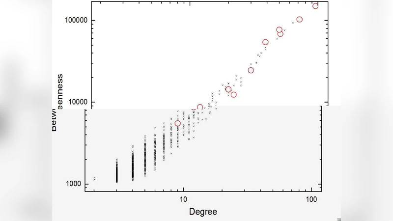
Impact of topology. By analytically and numerically investigating networks with heterogeneous degree distributions (e.g., scale‑free Barabási‑Albert graphs), the authors demonstrate that the placement of supply nodes dramatically influences (C). Concentrating supplies on high‑degree hubs creates heavily used corridors, lengthening many shortest paths and reducing overall capacity. Conversely, distributing supplies across lower‑degree vertices spreads traffic more evenly, shortening average routes and boosting (C). The effect is amplified in networks with strong degree heterogeneity, high clustering, or assortative mixing.

Optimization problem. Selecting the optimal subset (S) of size (M) that minimizes (C) is a combinatorial problem with (\binom{N}{M}) possibilities, infeasible for realistic sizes. The authors therefore adopt a meta‑heuristic approach based on Simulated Annealing (SA). An initial random configuration of supply nodes is generated, and at each iteration a pair of nodes (one supply, one non‑supply) is swapped. The new capacity (C’) is computed efficiently by re‑running Dijkstra’s algorithm from all demand nodes (or by incremental updates). If (C’) improves the objective, the move is accepted; otherwise it is accepted with probability (\exp