Computing the Solutions of the Combined Korteweg-de Vries Equation by Turing Machines

Differential equations are very popular mathematical models of real world problems. Not every differential equation has a well behaved solution. For those equations whose well behaved solutions exist, we are interested in how they can be computed. Thus, the computability of the solution operators for different types of nonlinear differential equations becomes one of the most exciting topics in effective analysis. This answers questions of the type: is it possible to calculate the solutions of some real word problems algorithmically? The answers to these questions are unfortunately not always positive. However, there are a lot of very interesting equations whose solutions do exist and can be calculated. These equations can be called computably solvable equations, in other words, their solution operators are computable. This means that, there are Turing machines which can transfer the initial data to the solutions of the equation in some particular spaces. For example, Klaus Weihrauch and Ning Zhong [7] have shown that the initial value problem of Korteweg-de Vries (KdV) equation posed on the real line R:

In this paper, we investigate a variation of Korteweg-de Vries equation: u t + uu x + u 2 u x + u xxx = 0. This is often called Combined Korteweg-de Vries (CKdV) equation. The Combined KdV equation is also an important equation which is frequently used as a mathematical model in physics, hydrodynamics, biological and chemical fields. We will show that the solution operator of the CKdV equation is also computable. This extends the results of [2,7]. The proof of the main theorem is given in Section 2.

In this section, we use a similar approach as that in [7] and retrieve two estimates to prove the main result. We use Type 2 theory of effectivity (TTE) as computation model. More relevant details can be found in [7].

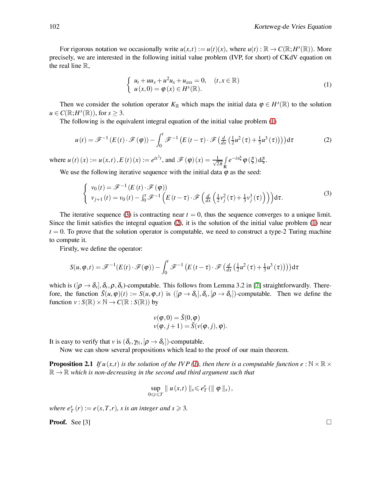
For rigorous notation we occasionally write u(x,t) := u(t)(x), where u(t) : R → C(R; H s (R)). More precisely, we are interested in the following initial value problem (IVP, for short) of CKdV equation on the real line R,

Then we consider the solution operator K R which maps the initial data ϕ ∈ H s (R) to the solution u ∈ C(R; H s (R)), for s ≥ 3.

The following is the equivalent integral equation of the initial value problem ( 1)

where u (t) (x) := u (x,t) , E (t) (x) := e ix 3 t , and

We use the following iterative sequence with the initial data ϕ as the seed:

The iterative sequence ( 3) is contracting near t = 0, thus the sequence converges to a unique limit. Since the limit satisfies the integral equation ( 2), it is the solution of the initial value problem (1) near t = 0. To prove that the solution operator is computable, we need to construct a type-2 Turing machine to compute it.

Firstly, we define the operator:

δ s , ρ, δ s )-computable. This follows from Lemma 3.2 in [7] straightforwardly. There- fore, the function S(u, ϕ)(t

Now we can show several propositions which lead to the proof of our main theorem.

) is the solution of the IV P (1), then there is a computable function e : N × R × R → R which is non-decreasing in the second and third argument such that

where e s T (r) := e (s, T, r), s is an integer and s 3.

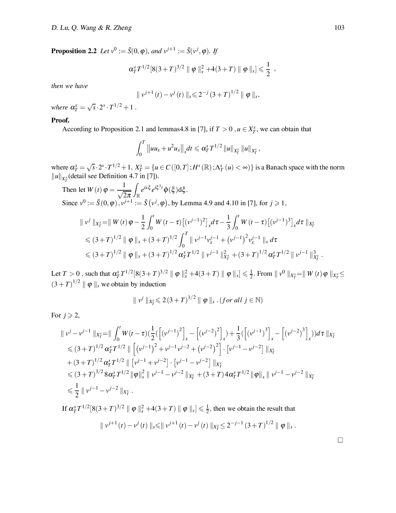
Proposition 2.2 Let v 0 := S(0, ϕ), and v j+1 := S(v j , ϕ). If

According to Proposition 2.1 and lemmas4.8 in [7], if T > 0 , u ∈ X s T , we can obtain that

where

e ixξ e iξ 3 t φ(ξ )dξ .

Since v 0 := S (0, ϕ) , v j+1 := S v j , ϕ , by Lemma 4.9 and 4.10 in [7], for j 1,

, then we obtain the result that

, by Lemma 4.8 in [7], we obtain the result as following:

Finally, we give the main results are as follows:

Proof. For a given initial value ϕ ∈ H s (R) and a rational number T > 0 we will show how to compute the solution u(t) of the initial value problem (1) at the time interval 0 t T . For this purpose, we first find some appropriate rational number T such that 0 < T < T , and show how to compute u(t) from t ′ and ψ := u(t ′ ) at the time interval [t ′ ,t ′ + T ], 0 t ′ T , by a fixed point iteration. Using this method, we can compute the values u (T /2m) successively for m = 1, 2, • • • and finally u (t) for any 0 t T . If u t + uu x + u 2 u x + u xxx = 0, u (x,t ′ ) = ψ (x), and v is defined by v (x,t) := u (x,t + t ′ ) , then

We assume that the initial value ψ ∈ H s (R) is given by a δH s -name, i.e., by a sequence ψ 0 , ψ 1 , • • • of Schwartz functions such that ψψ n s 2 -n . For any n ∈ N, we define function

We note that the sequence {v j n } can be computed from ψ n . By Proposition 3.3, the iterative sequence v 0 n , v 1 n , • • • converges to some v n , then v n is the fixed point of the iteration S and satisfies the following internal equation:

By Proposition 2.3, we will show that, by a contraction argument, for some sufficiently small computable real number T > 0 (depending only on ϕ and T ), v j n (t) → v n (t) as j → ∞ for all n, and v n (t) → v (t) as n → ∞, sufficiently fast and uniformly in t ∈ [0, T ]. We recall that v is the solution of

…(Full text truncated)…

This content is AI-processed based on ArXiv data.