A numerical closure approach for kinetic models of polymeric fluids: exploring closure relations for FENE dumbbells
We propose a numerical procedure to study closure approximations for FENE dumbbells in terms of chosen macroscopic state variables, enabling to test straightforwardly which macroscopic state variables should be included to build good closures. The me…
Authors: ** 제공된 텍스트에는 저자 정보가 명시되어 있지 않습니다. (원문에서 저자명을 확인할 수 없는 경우, 논문 PDF 혹은 출판사 페이지를 참고하시기 바랍니다.) **
A n umerical closure approac h for kinetic mo dels of p olymeric fluids: exploring closure relations for FENE dum bb ells Gio v anni Samaey ∗ , T on y Leli` evre † and Vincent Legat ‡ April 11, 2019 Abstract W e propose a n umerical procedure to study closure approximations for FENE dum b- b ells in terms of chosen macroscopic state v ariables, enabling to test straigh tforwardly whic h macroscopic state v ariables should be included to build go o d closures. The metho d inv olves the reconstruction of a p olymer distribution related to the conditional equilibrium of a microscopic Mon te Carlo simulation, conditioned up on the desired macroscopic state. W e describe the pro cedure in detail, give numerical results for sev eral strategies to define the set of macroscopic state v ariables, and sho w that the resulting closures are related to those obtained by a so-called quasi-equilibrium appro x- imation [ 19 ]. 1 In tro duction The simulation of dilute solutions of p olymers in a Newtonian solven t is a challenging mo d- elling and n umerical problem, since deformation of the p olymer molecules causes stresses that result in macroscopic non-Newtonian rheological b eha vior. One approach is to couple the macroscopic fluid flo w equations to a microscopic mo del for the polymers, a so-called micro-macro mo del [ 15 , 27 , 28 ]. The simplest microscopic mo dels, that we will use in this pap er, describ e the individual p olymers as non-in teracting dum bb ells, consisting of t wo b eads connected by a spring that mo dels intramolecular interaction. The state of the p olymer c hain is described b y the end-to-end v ector X t that connects b oth b eads whose ∗ Departmen t of Computer Science, K.U. Leuv en, Celestijnenlaan 200A, B-3001 Leuv en, Belgium giovanni.samaey@cs.kuleuven.be † CERMICS, Ecole des Pon ts P arisT ec h, 6 et 8 av en ue Blaise Pascal, Cit Descartes - Champs sur Marne, 77455 Marne la V alle Cedex 2, F rance lelievre@cermics.enpc.fr ‡ Departmen t of Mechanical Engineering and iMMC, U.C. Louv ain, Aven ue Georges Lematre, 4, B-1348 Louv ain-la-Neuv e, Belgium vincent.legat@uclouvain.be 1 ev olution is mo delled using a sto c hastic differential equation (SDE): d X t + u · ∇ x X t dt = ∇ x uX t − 2 ζ F ( X t ) dt + s 4 k B T ζ d W t , (1.1) where u is the v elo cit y field of the solven t, ζ is a friction co efficien t, T is the temp erature, k B is the Boltzmann constant, and W t is a standard multidimensional Brownian motion. This mo del takes into account Stokes drag (due to the solv ent velocity field), a spring force F and Bro wnian motion (due to collisions with solv en t molecules). The left-hand side of Equation ( 1.1 ) is the conv ectiv e deriv ative. Note that the sto c hastic pro cess X t implicitly dep ends on the space v ariable x . T o sp ecify the microscopic mo del ( 1.1 ) completely , we need to define the spring force. This force can b e more or less complicated, depending on the effects taken into accoun t. The simplest mo del is the Ho okean dumbbell mo del for which the spring is linear elastic: F ( X ) = H X , with H a spring constant. Another mo del, which is the fo cus of this pap er and which is kno wn to yield b etter agreement with exp erimen ts, is the finitely extensible nonlinear elastic (FENE) force [ 4 ]: F ( X ) = H X 1 − k X k 2 / ( bk B T /H ) , (1.2) where b is a nondimensional parameter related to the maximal p olymer length. In the macroscopic part of the mo del, the ev olution of the solven t velocity and pressure fields u and p is mo deled by mass and momentum conserv ation equations: ρ ∂ u ∂ t + u · ∇ x u = η s ∆ x u − ∇ x p + div x ( τ p ) , div x ( u ) = 0 , (1.3) with ρ the densit y and η s the viscosit y . Equation ( 1.3 ) contains an additional stress tensor τ p due to p olymer deformation, which is giv en via the classical Kramers’ expression τ p ( x, t ) = n h X t ⊗ F ( X t ) i − nk B T Id . (1.4) Here, n is the polymer concentration and h·i denotes the expectation ov er configuration space, which is approximated in practice by an empirical mean ov er a very large ensemble of realizations of X t , solutions to ( 1.1 ). One thus obtains a coupled system ( 1.1 )–( 1.3 )–( 1.4 ) that we rewrite in a non-dimensional 2 form as (see for example [ 20 ]): Re ∂ u ∂ t + u · ∇ x u = (1 − )∆ x u − ∇ x p + div x ( τ p ) , (1.5) div( u ) = 0 , (1.6) τ p = W e h X t ⊗ F ( X t ) i − Id , (1.7) d X t + u · ∇ x X t dt = ∇ x u X t − 1 2W e F ( X t ) dt + 1 √ W e d W t , (1.8) where the nondimensional parameters are: Re = ρU L η , W e = λU L , = η p η . (1.9) Here, U is a characteristic velocity , L = p k B T /H denotes a characteristic length, λ = ζ / 4 H is a c haracteristic relaxation time for the polymers and η p = nk B T λ is a viscosit y associated to the p olymers. The total viscosity is η = η p + η s . The parameters Re and W e are the Reynolds and W eissenberg num b er, resp ectively . The nondimensional Ho ok ean and FENE forces write resp ectiv ely: F H O OK ( X ) = X , F F E N E ( X ) = X 1 − k X k 2 /b . (1.10) The microscopic part of the mo del, i.e. ( 1.7 )–( 1.8 ), can equiv alen tly b e describ ed b y a diffusion equation that go v erns the evolution of the probability distribution ϕ ( X , x, t ) of the random v ariable X t (considered at p oin t x in physical space): ∂ ϕ ∂ t + u · ∇ x ϕ = 1 2W e ∆ X ϕ − div X ( ∇ x u X ϕ ) + 1 2W e div X ( F ( X ) ϕ ) , (1.11) The exp ectation in ( 1.7 ) then b ecomes an av erage with resp ect to the probability measure ϕ ( X , x, t ) d X : τ p ( x, t ) = W e Z X ⊗ F ( X ) ϕ ( X , x, t ) d X − Id . (1.12) W e refer for example to [ 4 , 8 , 34 ] for more details on the physical background and more complicated mo dels. A n umerical simulation of the coupled system ( 1.5 )–( 1.8 ) is v ery exp ensive, since one needs to obtain the non-Newtonian stress tensor τ p at eac h space-time discretization no de. Sev eral approaches hav e b een prop osed in the literature [ 23 , 28 ]. A first approac h is a de- terministic micro-macro simulation. Here, one couples the F okker–Planc k equation ( 1.11 )– ( 1.12 ) with the Navier–Stok es equations ( 1.5 )–( 1.6 ). The main dra wback of these metho ds is their high computational cost, due to the high-dimensionality of the function ϕ (which dep ends on sev en scalar v ariables ( X , x, t ) in dimension 3). This difficulty b ecomes all the more severe when more refined mo dels inv olving higher dimensional microscopic v ariables X t are used to describ e the polymers. Sp ecialized tec hniques are curren tly b eing dev elop ed; 3 see e.g. [ 1 , 2 , 7 ]. The micro-macro sim ulation can also be p erformed sto c hastically . One then discretizes the macroscopic fields (velocity , pressure, stress) on a mesh, and supplemen ts the (macroscopic) discretization of the Navier-Stok es equations with a sto c hastic simulation of an ensemble of p olymers using a discretization of the SDE ( 1.8 ), see [ 15 , 27 ]. Metho ds ha ve b een prop osed to obtain sufficiently lo w-v ariance results [ 6 , 15 , 20 ]. Due to the very high computational cost of micro-macro sim ulations, another route whic h has b een follo w ed (see e.g. [ 14 , 16 , 22 , 32 , 33 , 35 ]) is to lo ok for an appro ximate closure at the macroscopic lev el, namely a mo del of the form: ∂ M ∂ t + u · ∇ x M = H ( M , ∇ x u ) , (1.13) τ p = T ( M ) , (1.14) whic h is close to the microscopic mo del ( 1.7 )–( 1.8 ). Here M denotes an ensem ble of macro- scopic state v ariables that dep end on time and space. A basic example of such a macro- scopic mo del is the Oldroyd-B mo del [ 4 ], whic h is actually equiv alent to the microscopic mo del ( 1.7 )–( 1.8 ) for a linear force F ( X ) = F H O OK = X . In this case, one can obtain a closed equation on the so-called conformation tensor σ ( t ) = ( σ i,j ( t )) d i,j =1 , with d the num- b er of space dimensions, and σ i,j ( t ) = h ( X i ) t ( X j ) t i , in which ( X i ) t , resp. ( X j ) t , represent the corresp onding comp onen t of X t . This yields the equation : ∂ t τ p + u · ∇ x τ p = ∇ x u τ p + τ p ∇ x u T + W e ( ∇ x u + ∇ x u T ) − 1 W e τ p . On the other hand, for the FENE mo del, no equiv alen t closed macroscopic mo del is known, and one has to resort to approximate closures to obtain macroscopic equations (see Sec- tion 2.2 ). The basic idea is to appro ximate the p olymer distribution b y a so-called c anonic al distribution function , whic h is determined using only the macroscopic state v ariables M (t ypically lo w-order momen ts of the distribution). The microscopic evolution law ( 1.8 ) (or ( 1.11 )) is then replaced b y a set of equations ( 1.13 ) for the evolution of the macroscopic state v ariables M , combined with a constitutiv e equation ( 1.14 ) for the stress. While such appro ximate macroscopic mo dels are desirable, at least from a computational p oin t of view, it is how ev er not alwa ys clear how to quan tify the effects of the in tro duced approximations on the accuracy of the simulation, and how to choose the macroscopic state v ariables M . Recen tly , there has b een quite some interest in the dev elopment of computational meth- o ds that aim at accelerating micro-macro simulation using on-the-fly numerical closure appro ximations. W e mention equation-free [ 24 , 25 ] and heterogeneous m ultiscale metho ds (HMM) [ 10 , 11 ]. In both approac hes, a crucial step is to define an op erator that generates a microscopic state corresp onding to a given macroscopic state; this is actually equiv alen t to prescribing the closure appro ximation. This step is called lifting in the equation-free frame- w ork, and r e c onstruction in HMM. Inspired by these metho ds, the present pap er studies in detail the question of lifting/reconstruction for the particular problem of micro-macro 4 mo dels for p olymeric fluids; the pro cedure we prop ose, how ever, could b e applied to many m ultiscale models. Sp ecifically , w e propose a computational procedure to reconstruct an ensem ble of N p olymers consistently with a given macroscopic state M , and w e exam- ine the errors that are in tro duced in the macroscopic ev olution by numeric al ly enfor cing closur e up on the selected macroscopic state v ariables. F or conv enience of exp osition and illustration, we restrict ourselves to one-dimensional simulations with pre-imp osed (time- dep enden t) velocity fields, i.e. equations ( 1.7 )–( 1.8 ) with given u ( x, t ), at one sp ecific p oin t x in space. Ho w ever, we emphasize that the numerical metho d can be used lik ewise for 2D or 3D situations, as well as for the closure approximation for the coupled problem ( 1.5 )–( 1.8 ). The main contributions of the present pap er are tw ofold: • F rom a mo delling viewp oint, w e prop ose a numerical closure strategy that enables to easily explore which sets of macroscopic state v ariables should b e chosen to get go od closure approximations. V arious strategies are prop osed and tested. • F rom a theoretical viewp oin t, we sho w the relation b et w een this n umerical closure strategy and the so-called quasi-equilibrium metho d prop osed in [ 19 ], whic h relies on an entrop y minimization principle. The pap er is organized as follows. In Section 2 , w e giv e some more detail on the FENE mo del and the existing literature on closure appro ximations. In Section 3 , w e prop ose a numerical closure approximation based on constrained SDE simulations [ 29 ], which is v ery flexible, and enables to explore the error introduced by the closure for v arious sets of macroscopic state v ariables M . This n umerical closure appro ximation is sho wn to b e optimal in the sense that, when applied to a microscopic model which has an equiv alen t macroscopic mo del, it indeed yields the macroscopic mo del (Section 4 ). Moreov er, we show in Section 5 that, in some sp ecific cases, it is closely related to the closure approximation based on a quasi-equilibrium condition in tro duced in [ 19 ]. Finally , we test the n umerical closure using a n umber of different strategies to define the macroscopic state v ariables M (Section 6 ). W e first p erform n umerical experiments to assess the capability of the selected macroscopic state v ariables to r e c over the desir e d p olymer distributions in strong flo w regimes. Second, we study if the pro cedure is able to c orr e ctly c aptur e macr osc opic evolution . While accelerating microscopic simulation is not the primary purp ose of the presen t pap er, w e give some remarks in this resp ect in Section 7 , where we briefly discuss the main results and giv e some directions for future research. 5 2 The FENE mo del and closure appro ximations 2.1 FENE dumbbells: discretization and a one-dimensional v ersion As mentioned ab o ve, we consider p olymer simulations with FENE dumbbells sub ject to a pre-imp osed (time-dep enden t) velocity field. Thus, in the remainder of the pap er, unless explicitly stated otherwise, the force is the FENE force, see ( 1.10 ) : F = F F E N E . Using the characteristic metho d to in tegrate the conv ectiv e deriv ativ e in ( 1.8 ) (Lagrangian frame), the equations of in terest reduce to: τ p = W e h X t ⊗ F ( X t ) i − Id , d X t = κ ( t ) X t − 1 2W e F ( X t ) dt + 1 √ W e d W t , (2.1) where X t no w dep ends on the fo ot of the characteristic rather than on the Eulerian space p osition x , and κ is the velocity gradien t (along the tra jectory). Unless stated otherwise, w e will w ork with a one-dimensional version of this equation, τ p = W e h X t F ( X t ) i − 1 , dX t = κ ( t ) X t − 1 2W e F ( X t ) dt + 1 √ W e dW t , (2.2) k eeping in mind that the algorithm, as well as its analysis and implementation extend straigh tforwardly to higher dimensions. Note that κ ( t ) is here a giv en one-dimensional time- dep enden t function and F denotes a one-dimensional version of the FENE force, see ( 1.10 ), namely F ( X ) = X 1 − X 2 /b . Suc h a one-dimensional framew ork has also b een used in [ 22 ] for example, to assess the influence of the Peterlin appro ximation (see Section 2.2 ) on transient b eha viour. Concerning discretization metho ds, w e use a classical Euler-Maruy ama scheme [ 26 ] with a Monte Carlo metho d: τ k p = W e 1 N N X n =1 X n,k F ( X n,k ) − 1 ! , X n,k +1 = X n,k + κ ( t k ) X n,k − 1 2W e F ( X n,k ) δ t + 1 √ W e √ δ t ξ n,k , (2.3) where the indices n and k denote resp ectively realization index and time index, t k = k δ t and ξ n,k are i.i.d. normal random v ariables. 6 F or conv enience, we in tro duce a short-hand notation for the discretization sc heme of the SDE in ( 2.3 ), X k +1 = s X ( X k , κ ( t k ) , δ t ) , (2.4) where X = { X n } N n =1 is the ensemble of N realizations, and κ ( t k ) indicates explicitly the v alue of the velocity gradient in ( 2.3 ) that is considered o ver the time interv al of size δ t . Theoretically , it can be sho wn that (for sufficien tly large b ), the norm of the end-to- end v ector in ( 1.8 ) or ( 2.2 ) (recall that F = F F E N E ) cannot exceed the maximal v alue √ b [ 21 ]. How ev er, the discretization sc heme ( 2.3 ) might yield spring lengths b eyond this maximal v alue. There are tw o w ays to deal with this problem [ 34 , Section 4.3.2]. The first is via an accept-reject metho d, in which, for each p olymer, the state after each time step is rejected if | X | 2 > (1 − √ δ t ) b , and a new random num b er is tried until acceptance. Alternativ ely , one could use a semi-implicit predictor-corrector metho d. In this text, w e c ho ose the accept-reject strategy . 2.2 Closure approximations for FENE dum bb ells W e no w briefly discuss the deriv ation of closure approximations of the type ( 1.13 )-( 1.14 ) for the FENE mo del. One closure appro ximation is the P eterlin pre-av eraging [ 5 ]. Here, one constructs an appro ximation for the FENE mo del by defining the spring force as (compare with ( 1.10 )) F F E N E − P ( X ) = X 1 − h X 2 i /b . (2.5) As a consequence, only the mean square length of the ensemble of polymers is constrained to remain smaller than √ b , whereas the length of individual p olymers may exceed this v alue. The in terest of FENE-P dum bb ells is that, as for Hookean dumbbells, a closed equation can b e deriv ed on the conformation tensor σ = h X 2 t i , and th us a macroscopic mo del is obtained: ∂ t σ + u ∇ x σ = 2 σ ∇ x u − 1 W e σ 1 − tr( σ ) /b + 1 W e . τ p = W e σ 1 − tr( σ ) /b − 1 , (2.6) It has b een shown in [ 14 , 22 ] that the Peterlin approximation has a profound impact on transien t b ehaviour in complex flo ws, compared to the original FENE mo del. Let us no w discuss more generally closure approximations of the type ( 1.13 ). F or the sak e of clarity , and without loss of generality , we restrict ourselves to the one-dimensional case ( 2.2 ). Consider starting from a num b er L of macroscopic state v ariables, M = { M l } L l =1 , which are defined as configuration space av erages of functions m l of the configuration X t , M l ( t ) = h m l ( X t ) i . (2.7) 7 The goal is to obtain a closed system of L evolution equations ( 1.13 ) for the state v ari- ables M , complemented with a constitutiv e equation ( 1.14 ) for τ p as a function of these macroscopic state v ariables. Using Itˆ o calculus, one can easily obtain the following equation of state for the macro- scopic state v ariables, dM l dt = κ ( t ) X t dm l dX ( X t ) | {z } M D l − 1 2W e F ( X t ) dm l dX ( X t ) | {z } M C l + 1 2W e d 2 m l dX 2 ( X t ) | {z } M B l , (2.8) in which the macroscopic state v ariables M { D,C ,B } l accoun t for hydrodynamic drag, connec- tor force and Brownian motion, resp ectively . Of course, in general, man y of these macro- scopic state v ariables M { D,C ,B } l are not functions of the initially chosen macroscopic state v ariables { M l } L l =1 . One can write evolution equations for these new state v ariables, which in turn will create additional state v ariables but this pro cedure typically go es on endlessly . A t some p oint, one has to stop, and try to approximate the state v ariables for which no ev olution equation is av ailable by writing them as a function of other (already av ailable) state v ariables. By adding suc h closur e r elations , one obtains an explicit, but approximate, closed system of evolution equations. An y closed macroscopic mo del needs to (i) define the set of macroscopic state v ariables M = { M l } L l =1 , and (ii) provide a wa y of ev aluating the remaining state v ariables M { D,C ,B } l in the ev olution equation as a function of M . In the literature, item (i) is generally addressed b y considering a hierarch y of even momen ts, i.e. M l = h X 2 l i where l = 1 , . . . , L (all the o dd moments are zero for reasons of symmetry). Note that these b ecome tensors in higher space dimensions. The corresp onding evolution equations ( 2.8 ) are then given as: dM l dt = 2 l κ ( t ) M l − 1 2W e M C l + l (2 l − 1) W e M l − 1 , (2.9) with M 0 = 1. In order to complete (ii), one needs to provide appro ximations for the new additional macroscopic state v ariables M C l L l =1 . Note that, in particular, one of this new additional macroscopic v ariable M C 1 is also required to obtain the constitutive relation ( 1.14 ) for τ p . One strategy to approximate M C l L l =1 is to prop ose a probability distribution ϕ M ( X ) (called a c anonic al distribution function ) that is parameterized b y the selected macroscopic state v ariables, and to compute M C l L l =1 in the evolution equations ( 2.8 ) as the exp ectation with resp ect to this canonical distribution function. Note that ϕ M ( X ) depends on time only through the dependency of M on the time v ariable. The rationale b ehind this approac h is that the b etter one can appro ximate the microscopic distribution function, the more reliable the obtained macroscopic mo del should b e. In [ 32 , 33 ], appro ximate closures for M C l are obtained by restricting the space of ad- missible distribution functions to linear com binations of L c anonic al b asis functions . Based on this approach, several closures ha ve b een prop osed; see [ 32 ] for more details on the 8 one-dimensional setting ( 2.2 ) and [ 33 ] for the general three-dimensional case. A related approac h is describ ed in [ 9 , 16 , 36 ]. Another route is describ ed in the following section. 2.3 Quasi-equilibrium approximations A particularly interesting approac h is prop osed in [ 19 ]. It consists in defining a so-called quasi-equilibrium canonical distribution function ϕ QE M via a constrained entrop y optimiza- tion problem: ϕ QE M = argmin ϕ ∈ Ω M Z ϕ ln ϕ ϕ eq , (2.10) where Ω M is defined as the set of all probability density functions, for which the a verage of m l is indeed M l : Ω M = ϕ ( X ) , ϕ ≥ 0 , Z ϕ ( X ) dX = 1 , Z m l ( X ) ϕ ( X ) dX = M l , l = 1 , . . . , L . (2.11) In ( 2.10 ), ϕ eq is defined as the equilibrium distribution for the p olymer configuration, for zero velocity field. In particular, for FENE dumbbells, it writes: ϕ eq ( X ) = Z − 1 1 − X 2 /b b/ 2 , where Z = Z | X |≤ √ b 1 − X 2 /b b/ 2 dX . The rationale b ehind this appro ximation is to assume a separation of time scales be- t ween the (supp osedly fast) relaxation tow ards the quasi-equilibrium distribution and the (supp osedly m uch slow er) evolution of the macroscopic state v ariables. An explicit expression of the solution to ( 2.10 ) can b e obtained as: ϕ QE M ( X ) = Z − 1 M ϕ eq ( X ) exp L X l =1 λ l m l ( X ) ! , (2.12) where Z QE M = Z ϕ eq ( X ) exp L X l =1 λ l m l ( X ) ! dX and the set of Lagrange m ultipliers Λ = { λ l } L l =1 are determined by the constrain ts Z m l ( X ) ϕ QE M ( X ) dX = M l . While the Lagrange multipliers dep end only on the macroscopic state M , the relation Λ( M ) can often not b e obtained analytically . Therefore, in [ 19 ], a n umerical pro cedure is prop osed to sim ulate the resulting closed macroscopic mo del. W e will show b elo w (see Sec- tion 5 ) that the numerical closure approximation technique that we prop ose (see Section 3 ) is closely related to this metho d, and that it may b e considered (for a slightly mo dified ver- sion) as a different n umerical strategy to obtain quasi-equilibrium closure appro ximations. 9 3 Numerical metho d In this section, we prop ose to mimic the evolution of the corresp onding unav ailable macro- scopic mo del via a c o arse time-stepp er [ 24 , 25 ]. 3.1 The lifting and restriction op erators Consider the ev olution of an ensemble of p olymers in a pre-imp osed velocity field and define a set of macroscopic state v ariables M which are believed to represen t the underlying (microscopic) p olymer distribution sufficiently accurately . W e introduce t wo op erators that mak e the transition betw een microscopic and macroscopic state v ariables. W e define a lifting op er ator , L : M 7→ X , (3.1) whic h maps a macroscopic state to an ensem ble of N p olymer configurations, and the asso ciated r estriction op er ator , R : X 7→ M , (3.2) whic h maps an ensem ble of configurations to the corresponding macroscopic state. Note that w e directly define the metho d at the discrete lev el o ver an ensem ble of N configurations (after Mon te Carlo discretization). F or a discussion in the limit of an infinitely large n um b er of p olymer configurations, we refer to Section 3.3 . The restriction op erator is readily defined using an empirical mean: R ( X ) = { M l = R l ( X ) } L l =1 with R l ( X ) = 1 N N X n =1 m l ( X n ) for l = 1 , . . . , L, (3.3) where, we recall, X = { X n } N n =1 denotes the ensemble of configurations. In the lifting step, w e need to sample a reconstructed p olymer distribution function, consisten tly with the giv en macroscopic state M ( t ∗ ) obtained at time t ∗ . T o this end, w e p erform a c onstr aine d simulation of an ensemble of p olymers until e quilibrium , sub ject to the constrain t that the macroscopic state remains constant and equal to M ( t ∗ ). More precisely , the constrained algorithm writes [ 29 ]: X m +1 = s X ( X m , κ ( t ∗ ) , δ t ) + L X l =1 λ l ∇ X R l ( X m ) , with Λ ∈ R L suc h that R l ( X m +1 ) = M l ( t ∗ ) for l = 1 , . . . , L . (3.4) It th us consists successively in an unconstrained Euler-Maruyama step, follow ed b y a pro- jection step to satisfy the constraint. In eac h constrained time step, the pro jection is done b y solving the nonlinear system R l X m +1 (Λ; X m , δ t ) = M l ( t ∗ ) , for l = 1 , . . . , L, (3.5) 10 for the unknown Lagrange multipliers Λ using Newton’s metho d. In ( 3.5 ), we hav e made explicit that the state X m +1 dep ends on the unkno wn Lagrange multipliers, as well as on (kno wn) X m and δ t . During the constrained simulation, an accept-reject strategy is applied on the combined ev olution and pro jection op eration, i.e. if, during pro jection, the state of a p olymer would b ecome unphysical, w e reject the trial mo ve in the unconstrained Euler- Maruy ama step and rep eat the time step for this p olymer, after which the pro jection of the ensem ble is tried again. The lifting op erator is then defined as the ensemble X m ∞ for a sufficiently large time index m ∞ , which is chosen suc h that ( 3.4 ) has reached an equilibrium distribution, L ( M ) = X m ∞ . (3.6) W e will detail further on how m ∞ is determined numerically when describing the computa- tional exp erimen ts. F or a precise definition of the lifting op erator in terms of distributions (in the limit of an infinite num b er of configurations), we refer to Section 3.3 . Of course, by construction one has the consistency prop ert y R ◦ L = Id . 3.2 The numerical closure algorithm Let us now make precise the complete algorithm. Given an initial condition for the macro- scopic state v ariables M ( t ∗ ) at time t ∗ , one time step of the coarse time-stepp er consists of a three-step pro cedure: (i) Lifting , i.e. the creation of initial conditions X ( t ∗ ) = L ( M ( t ∗ )) for the microscopic mo del, consistently with the macroscopic state M ( t ∗ ) at t ∗ . (ii) Simulation using the microscopic mo del ov er a time interv al [ t ∗ , t ∗ + K δ t ], where K is the num b er of time steps, to get X ( t ∗ + K δ t ): for k = 0 , . . . , K − 1, X ( t ∗ + ( k + 1) δ t ) = s X ( X ( t ∗ + k δ t ) , κ ( t ∗ + k δ t ) , δ t ) . (iii) R estriction , i.e. the observ ation (estimation) of the macroscopic state at t ∗ + K δ t : M ( t ∗ + K δ t ) = R ( X ( t ∗ + K δ t )) . In the following, we denote ∆ t = K δ t. 11 During the restriction step, the ensemble X ( t ∗ + ∆ t ) is also used to get an estimate of the new v alue of the stress τ p ( t ∗ + ∆ t ) = W e 1 N N X n =1 X n ( t ∗ + ∆ t ) F ( X n ( t ∗ + ∆ t )) − 1 ! . 3.3 The lifting and restriction op erator in the con tin uous limit The lifting and restriction op erators which hav e b een defined ab ov e dep end on three dis- cretization parameters: N which is related to the Monte Carlo discretization (the op erators ha ve b een defined for a finite ensemble of configurations), δ t which is related to the time discretization in ( 3.4 ), and m ∞ whic h should b e sufficien tly large to reac h a stationary state in ( 3.4 ). In this section, we introduce the limiting op erators L and R obtained in the limit N → ∞ , δ t → 0 and m ∞ δ t → ∞ . Note first that these op erators are well-defined in terms of the probability distribution ϕ , rather than ensembles of configurations. More precisely , the lifting operator L con- sists in constructing a probability distribution ϕ N C M consisten tly with the macroscopic state v ariables M (using the notation of Sections 2.2 - 2.3 ), L ( M ) = ϕ N C M ( X ) , (3.7) in whic h the superscript N C stands for numeric al closur e . Likewise, the restriction op erator R reduces a distribution to macroscopic state v ariables. The restriction op erator R is simply an a v eraging op erator, whic h computes the av erages of m i with resp ect to the distribution ϕ (compare with ( 3.3 )): R ( ϕ ) = { M l = R l ( ϕ ) } L l =1 with R l ( ϕ ) = Z m l ϕ for l = 1 , . . . , L, (3.8) On the other hand, the lifting op erator L is more in volv ed to define. When considering the contin uous-in-time version of ( 3.4 ) in the limit of an infinite num b er of configurations, N → ∞ , it can b e seen to b e giv en b y the one-dimensional marginal of the stationary state of the asso ciated F okker-Planc k equation. Let us make this statement precise. F or a fixed v alue N , the numerical scheme ( 2.3 ) is a discretization of the following constrained Stratono vitc h SDE on the ensem ble X t = { X n t } N n =1 (see [ 29 ] and [ 30 , Chapter 3]): d X t = P ( X t ) κ ( t ∗ ) X t − 1 2W e F ( X t ) dt + 1 √ W e P ( X t ) ◦ d W t , (3.9) where, with a slight abuse of notation, F ( X t ) ≡ ( F ( X n t )) N n =1 , and W t represen ts an N - dimensional Brownian motion. The pro jection op erator P ( X t ) is defined by: P ( X ) = Id − L X i,j =1 G − 1 i,j ( X ) ∇ X R i ( X ) ⊗ ∇ X R j ( X ) 12 with G − 1 i,j ( X ) the inv erse of the Gram matrix: G i,j ( X ) = ∇ X R i ( X ) · ∇ X R j ( X ) and ◦ denotes the Stratono vitch pro duct. If we denote Σ( M ) = {X , R ( X ) = M } (3.10) the submanifold of X at fixed v alues of the macroscopic state v ariables, then P ( X ) is the orthogonal pro jection op erator on to the tangent space T X Σ( M ) of Σ( M ) at p oin t X . Th us, if X 0 ∈ Σ( M ), then, for all t ≥ 0, X t ∈ Σ( M ). Let us denote ψ N ( t, d X ) the distribution of X t satisfying ( 3.9 ). Note that the comp o- nen ts of X t ha ve all the same law, for symmetry reasons. Let us introduce the marginal of ψ N in the first v ariable: ψ N 1 ( t, X 1 ) dX 1 = Z X 2 ,...,X N ψ N ( t, dX 1 , . . . , dX N ) . (3.11) Then, ϕ N C M is defined as: ϕ N C M ( X ) = lim N →∞ lim t →∞ ψ N 1 ( t, X ) . (3.12) By a la w of large n umbers, it is exp ected that this distribution ϕ N C M is consistent with the fixed v alues of macroscopic state v ariables M : ϕ N C M ∈ Ω M , where Ω M is defined by ( 2.11 ). W e will discuss in Section 5 how to get an analytical expression for ϕ N C M , at least in some sp ecific cases. 3.4 Choice of the macroscopic state v ariables F or the FENE mo del, it app ears that the first even moment h X 2 t i is not sufficient to char- acterize the p olymer distribution, and additional macroscopic state v ariables are needed. W e will consider the macroscopic level to b e determined by L macroscopic state v ariables, M = { M l } L l =1 , and we consider the following strategies to select M l , l = 1 , . . . , L . Strategy 1. W e consider a hierarch y of even moments of increasing order, M l = h X 2 l t i , l = 1 , . . . , L. (3.13) 13 Strategy 2. W e consider a hierarc h y of ev en momen ts of increasing order, and supplement the set of macroscopic state v ariables with the additional momen ts that app ear in the corresp onding ev olution equations ( 2.9 ), ( M l = h X 2 l t i , M ˜ L/ 2+ l = M C l = 2 l h F ( X t ) X 2 l − 1 t i , (3.14) for 1 ≤ l ≤ ˜ L/ 2 where ˜ L is assumed to be ev en. F or FENE dum bbells, it can easily b e c heck ed that τ p = W e M C 1 / 2 − 1 , and that all M C l , l > 1 can b e written as linear combinations of M l , l = 1 , . . . , ˜ L/ 2 and τ p . Hence, this choice is equiv alen t to taking M l = h X 2 l t i , l = 1 , . . . L − 1 M L = τ p = W e ( h X t F ( X t ) i − 1) = W e X 2 t 1 − X 2 t /b − 1 , (3.15) where L = ˜ L/ 2 + 1 denotes the n umber of linearly indep endent macroscopic state v ariables. Strategy 3. W e again start from M 1 = h X 2 t i . T o add state v ariables, w e write down the ev olution equation for M 1 , i.e. ( 2.9 ) with l = 1, and add all macroscopic state v ariables that app ear in this equation. In this case, this amoun ts to adding the v ariable M 2 = M C 1 . W e contin ue b y writing down the evolution equation ( 2.8 ) for M 2 , which, in turn, reveals additional state v ariables M D,C ,B 2 . Some elemen tary algebra shows that we obtain four linearly indep enden t macroscopic state v ariables: M 1 = h X 2 t i , M 2 = X 2 t 1 − X 2 t /b − 1 , (3.16) as ab o ve, and additionally M 3 = X 2 t (1 − X 2 t /b ) 2 , M 4 = X 4 t (1 − X 2 t /b ) 3 . (3.17) Note that these same macroscopic state v ariables would also show up after simplification b y applying this pro cedure starting from the choice M 1 = τ p . If additional moments are desired, one could con tinue by writing down evolution equations for M 3 and M 4 and add the moments that appear in those equations, but we will not consider that in the remainder of the text. 4 A consistency result for FENE-P dum bb ells T o chec k the consistency of the whole procedure, let us apply the n umerical closure ap- pro ximation to the case of FENE-P dum bb ells (namely using the spring force ( 2.5 )). In 14 this case, it is known that there exists a macroscopic equiv alen t mo del and the question is th us: do w e recov er this macroscopic mo del using the numerical closure pro cedure ? W e first derive a theoretical result, which we subsequently illustrate numerically . 4.1 A simple remark Let us consider the FENE-P mo del, with the ab o ve n umerical closure approximation metho d applied using only one macroscopic state v ariable M = h X 2 t i . Note that the stress τ p is defined in terms of M as τ p = W e M 1 − M /b − 1 . As mentioned ab o ve (see ( 2.6 )), for the microscopic mo del ( 2.2 ), M satisfies a closed equation: ∂ t M = 2 κM − 1 W e M 1 − M /b + 1 W e . (4.1) W e no w make a simple observ ation to show that the numerical closure approximation (in the limit of zero discretization errors) repro duces this macroscopic dynamics. W e refer to the notation of Section 3.2 . F or a given v alue of M ( t ∗ ) at time t ∗ , the lifting step (i) creates an ensem ble of configurations with, by construction, a la w ϕ N C M ( t ∗ ) = L ( M ( t ∗ )) suc h that Z X 2 ϕ N C M ( t ∗ ) ( X ) dX = M ( t ∗ ). But then, the simulation step (ii) will indeed propagate M according to ( 4.1 ) (which is deduced from ( 2.2 ) by a simple Itˆ o calculus). Thus, after the restriction step (iii), the correct v alues for M are recov ered. In conclusion, if there exists a closed macroscopic equation for the stress, the prop osed n umerical closure approximation indeed reco vers this macroscopic ev olution as so on as the appropriate macroscopic state v ariables are selected. 4.2 Numerical illustration W e consider one-dimensional FENE-P dumbbells, go vern ed by ( 2.2 ), in which the spring force F ( X ) ≡ F F E N E − P ( X ) is giv en by ( 2.5 ) with nondimensional parameters b = 49, W e = 1 and = 1. As in [ 22 ], we prescrib e the velocity field κ ( t ) = 100 t (1 − t ) exp( − 4 t ) . (4.2) The microscopic mo del ( 2.2 ) is discretized via the Euler-Maruy ama metho d with time step δ t = 10 − 2 . 4.2.1 Lifting T o illustrate that the macroscopic v ariable M = h X 2 t i uniquely determines the polymer distribution, we p erform the following exp erimen t. W e first simulate an ensem ble of N = 10 5 15 0 0 . 05 0 . 1 0 . 15 0 . 2 ϕ ( | X | ) 0 5 10 15 20 | X | mδ t = 0 mδ t = 5 mδ t = 15 mδ t = 50 reference Figure 1: Polymer distribution for FENE-P dumbbells during constrained simulation. Shown are the p olymer distribution b efore the restriction at t = 0 . 3 (the reference distribution), and at sev eral time instances during a constrained simulation starting from a uniform initial distribution. (The non-uniform app earance of the initial condition is due to artifacts of the binning.) Parameters of the simulation are giv en in the text. FENE-P dum bb ells, sub ject to the v elo city gradient κ ( t ) ov er the time in terv al t ∈ [0 , 0 . 3]. As the initial condition, w e take the equilibrium p olymer distribution in the absence of flo w. A t t = 0 . 3, we obtain M ∗ = M ( t = 0 . 3) via restriction; the corresp onding p olymer distribution is kept as the reference distribution. Next, we initialize a new ensemble of p olymers consistently with the macroscopic state M ∗ using a uniform distribution. W e then p erform a constrained simulation ( 3.4 ) using the same time-step δt ov er the constrained time in terv al [0 , m ∞ δ t ] = [0 , 50]. The results are shown in Figure 1 . W e see that the distribution of the constrained simulation conv erges tow ards the dis- tribution of the original sim ulation, indicating that the first ev en momen t M is indeed sufficien t to represent the original p olymer distribution, and also that the constrained sim- ulation recov ers this distribution. Note, ho wev er, that this exp erimen t rev eals an imp ortan t prop erty of FENE-P dumb- b ells. While the manifold consisting of Gaussian distributions with zero mean is invariant , there is no str ong time-sc ale sep ar ation b et ween the relaxation of arbitrary distributions with given second moment to wards the Gaussian distribution and evolution of this second momen t itself. This can b e concluded by noting that one needs to sim ulate the constrained SDE ov er a time interv al of length 50 to reac h the stationary distribution, whereas the macroscopic state v ariable evolv es significantly on considerably shorter time-scales, see also the next exp erimen t. This w as also observ ed in [ 17 ]. 16 0 100 200 300 400 500 τ p 0 10 20 30 40 50 M ∆ t = 1 δt ∆ t = 10 δt ∆ t = 50 δt reference 0 20 40 60 M 0 0 . 5 1 1 . 5 2 t 0 200 400 600 τ p Figure 2: Ev olution of the first even momen t M and stress τ p for an ensem ble of FENE-P dumbbells during complex flow. Left: ( M , τ p ) phase plane view. Right: temp oral evolution. Sho wn are a full microscopic sim ulation (reference), and simulations using a coarse time-stepp er for different v alues of the macroscopic time-step. Sim ulation parameters are given in the text. 4.2.2 Coarse time-stepping W e now look into the ev olution of the numerical closure with resp ect to the full microscopic sim ulation. T o this end, we simulate an ensemble of N = 2 · 10 4 FENE-P dumbbells, starting from the equilibrium distribution ϕ eq in the absence of flo w, up to time t = 2. All n umerical parameters are the same as ab o ve. In particular, κ ( t ) is again given by ( 4.2 ). W e compare this reference simulation with a num b er of simulations using the coarse time-stepp er with differen t v alues of the time step ∆ t = K δ t . In this exp erimen t, the lifting step amounts to freezing ph ysical time and p erforming a constrained simulation that is consistent with M . The constrained sim ulations are p erformed ov er a time interv al of size 100∆ t . The results are shown in Figure 2 . W e see that the results are nearly identical for all v alues of ∆ t and the results nearly coincide with the reference sim ulation. This is to b e exp ected. Indeed, since M completely determines the polymer distribution, a simulation constrained up on M will not alter this distribution, see Section 4.1 . 5 Comparison of numerical closure with quasi-equilibrium metho d In this section, w e compare the prop osed n umerical closure appro ximation (described in Section 3 ) with the quasi-equilibrium metho d prop osed in [ 19 ] (describ ed in Section 2.3 ). In particular, w e sho w that the quasi-equilibrium metho d, as proposed in [ 19 ], is equiv- 17 alen t to the numerical closure approximation, when the v elo cit y gradient κ ( t ∗ ) is tak en to zero in ( 3.4 ). T o prov e this result, we need to show that the canonical distribution ϕ QE M reconstructed from the quasi-equilibrium metho d (see Equation ( 2.12 )) is the same as the distribution ϕ N C M reconstructed from the lifting pro cedure through the op erator ¯ L (see Equations ( 3.7 ) and ( 3.12 )). Let us consider the microscopic mo del ( 1.7 )–( 1.8 ), with a general force F which derives from a p oten tial Π: F = ∇ Π , so that the equilibrium distribution (for zero velocity field) is ϕ eq = Z − 1 exp( − Π) , where Z = R exp( − Π). Let us consider a fixed given set of macroscopic state v ariables M , and, for the sak e of simplicity , let us assume that L = 1 (only one macroscopic state v ariable M is considered). F rom the quasi-equilibrium metho d, the reconstructed distribution is (see Equation ( 2.12 )): ϕ QE M ( X ) = Z QE M exp ( − Π( X ) + λm ( X )) , (5.1) where Z QE M = Z exp ( − Π( X ) + λ m ( X )) dX and the single Lagrange multiplier λ is deter- mined by the constraint Z m ( X ) ϕ QE M ( X ) dX = M . Let us now consider the numerical closure approximation describ ed in Section 3 , with κ ( t ∗ ) = 0 in ( 3.4 ). In this case, since κ ( t ∗ ) = 0 in ( 3.9 ), the stationary distribution for ( 3.9 ) has a simple expression: ψ N ( ∞ , d X ) = ( Z N ) − 1 N Y n =1 exp( − Π( X n )) dσ Σ( M ) , where σ Σ( M ) is the Leb esgue measure on the submanifold Σ( M ) defined b y ( 3.10 ). W e refer for example to [ 29 ] or [ 30 , Prop osition 3.20]. Then, the marginal ψ N 1 ( ∞ , X ) is defined through (see ( 3.11 )): ψ N 1 ( ∞ , X 1 ) dX 1 = Z X 2 ,...,X N ψ N ( ∞ , dX 1 , . . . , dX N ) , (5.2) and the reconstructed distribution from the numerical closure approximation is (see ( 3.12 )): ϕ N C M ( X ) = lim N →∞ ψ N 1 ( ∞ , X ) . (5.3) The main mathematical result of this work is the following: Prop osition 5.1. The r e c onstructe d distributions obtaine d thr ough the quasi-e quilibrium metho d, and the numeric al closur e appr oximation metho d with zer o gr adient velo city field ar e the same: ϕ QE M = ϕ N C M . 18 This prop osition is a corollary of a general result ab out the equiv alence (for an infinite n umber of particles) of the canonical ensemble and the micro canonical ensem ble in statistical ph ysics. W e cite a result from [ 3 , Theorem A.5.5], see also [ 13 , Theorem 3.4]: Theorem 5.2. L et α b e a pr ob ability me asur e on R d and let us c onsider Y 1 , . . . , Y N i.i.d. r andom variables with law α , and intr o duc e a function q : R d → R . L et us now define two pr ob ability me asur es: • The c onditional me asur e ν N | z dy 1 , . . . , dy N = α ⊗ N dy 1 , . . . , dy N 1 N N X n =1 q ( y n ) = z ! of the ve ctor ( Y 1 , ..., Y N ) c onditional ly to 1 N P N n =1 q ( Y n ) = z . • The pr ob ability me asur e α λ ( dy ) = Z − 1 λ exp( λq ( y )) α ( dy ) , wher e Z λ = R exp( λq ( y )) α ( dy ) . L et us assume that λ and z ar e r elate d thr ough the r elation: Z q ( y ) α λ ( dy ) = z . Then, one has: for any test function F : R d → R , lim N →∞ Z F ( y 1 ) ν N | z dy 1 , . . . , dy N = Z F ( y 1 ) α λ ( dy 1 ) . T o apply Theorem 5.2 to pro ve Prop osition 5.1 , we set α to b e the equilibrium distri- bution ϕ eq , q = m , and z = M . Then α λ = ϕ QE M , and it remains to show that lim N →∞ Z F ( y 1 ) ν N | z dy 1 , . . . , dy N = Z F ( y 1 ) ϕ N C M ( y 1 ) dy 1 . This is stated in the following lemma: Lemma 5.3. L et us c onsider the notation of The or em 5.2 and assume that the me asur e α has a density a : α ( dy ) = a ( y ) dy . L et us intr o duc e the pr ob ability me asur e ν N Σ( z ) ( dy 1 , . . . , dy N ) = a ( y 1 ) · · · a ( y N ) σ Σ N ( z ) ( dy 1 , . . . , dy N ) , wher e Σ N ( z ) = { ( y 1 , . . . , y N ) , 1 N P N n =1 q ( y n ) = z } and σ Σ N ( z ) is the L eb esgue me asur e on the submanifold Σ N ( z ) . Then, ν N Σ N ( z ) ( dy 1 , . . . , dy N ) = k∇ Q N k ν N | z dy 1 , . . . , dy N , (5.4) wher e Q N ( y 1 , . . . , y N ) = 1 N P N n =1 q ( y n ) . Mor e over, lim N →∞ Z F ( y 1 ) ν N | z dy 1 , . . . , dy N = lim N →∞ Z F ( y 1 ) ν N Σ N ( z ) dy 1 , . . . , dy N . (5.5) 19 Pr o of. The pro of of ( 5.4 ) is based on the co-area formula, see for example [ 30 , Eq. (3.14)]. Then, to pro v e ( 5.5 ), one notice that, if Y 1 , . . . Y N denotes random v ariables distributed according to the conditional probabilit y measure ν N | z , one has: Z F ( y 1 ) ν N Σ N ( z ) dy 1 , . . . , dy N = F ( Y 1 ) k∇ Q N k ( Y 1 , . . . , Y N ) hk∇ Q N k ( Y 1 , . . . , Y N ) i = F ( Y 1 ) q 1 N P N n =1 k∇ q k 2 ( Y n ) q 1 N P N n =1 k∇ q k 2 ( Y n ) . By a law of large num bers (see for example [ 3 , Theorem A.5.4] or [ 13 , Theorem 3.5]), 1 N N X n =1 k∇ q k 2 ( Y n ) conv erges in probabilit y to Z k∇ q k 2 dα λ , and th us, Slutsky lemma enables to conclude. This concludes the pro of of Prop osition 5.1 , since with the notation introduced ab o v e ( α ( dy ) = ϕ eq ( y ) dy , q = m , and z = M ) ν N Σ N ( z ) ( dy 1 , . . . , dy N ) = ψ N ( ∞ , dy 1 , . . . , dy N ) . A few remarks are in order. First, in dimension 1, the fact that the drift in the SDE deriv es from a p oten tial is not a restrictive assumption, so that the quasi-equilibrium pro- cedure could also be applied when taking in to account a non-zero κ ( t ∗ ). Ho wev er, this assumption is indeed restrictive in dimension greater than one: for non-symmetric κ ( t ∗ ), the drift in ( 2.1 ) is not the gradien t of a p oten tial. In this case, the numerical closure appro ximation pro cedure still applies, but it is unclear ho w it would b e related to a quasi- equilibrium metho d. In some sense, the numerical closure metho d can thus b e seen as a generalization of the quasi-equilibrium metho d, which tak es in to account the v elo cit y gradi- en t in the lifting procedure. In fact, the n umerical closure procedure can b e seen as a simple alternativ e to simulate the quasi-equilibrium closures that, unlike the numerical pro cedure in [ 19 ], does not require transformations from moments to Lagrange multipliers and vice v ersa, which migh t b e difficult to p erform. 6 Numerical illustrations for FENE dumbbells In this section, w e perform some n umerical experiments to explore the behaviour of the n umerical closure pro cedure using the strategies for macroscopic state v ariable detection that were outlined in Section 3.4 . 20 0 0 . 1 0 . 2 0 . 3 0 . 4 ϕ ( | X | ) 0 1 2 3 4 5 6 7 | X | L = 1 L = 2 L = 3 L = 4 reference 0 0 . 1 0 . 2 0 . 3 0 . 4 0 . 5 ϕ ( | X | ) 0 1 2 3 4 5 6 7 | X | L = 1 L = 2 L = 3 L = 4 reference 0 0 . 2 0 . 4 0 . 6 0 . 8 1 ϕ ( | X | ) 0 1 2 3 4 5 6 7 | X | L = 1 L = 2 L = 3 L = 4 reference 0 0 . 25 0 . 5 0 . 75 1 1 . 25 1 . 5 ϕ ( | X | ) 0 1 2 3 4 5 6 7 | X | L = 1 L = 2 L = 3 L = 4 reference Figure 3: Lifted polymer distributions for FENE dum bb ells as a function of the num b er of macro- scopic state v ariables using strategy 1. W e plot a reference p olymer distribution, that is obtained b y microscopic simulation up to time t ∗ , as w ell as the equilibrium p olymer distributions after con- strained simulation using L = 1 , . . . , 4 even momen ts. Shown are the results for t ∗ = 0 . 5 (top left), t ∗ = 1 (top righ t), t ∗ = 1 . 5 (b ottom left) and t ∗ = 2 (b ottom right). Simulation parameters are giv en in the text. 6.1 Strategy 1: Even moments as macroscopic state v ariables 6.1.1 Lifted configuration distributions W e sim ulate an ensemble of N = 5 · 10 4 FENE dumbbells, sub ject to a constant velocity gradien t κ ( t ) = 2 ov er the time in terv al t ∈ [0 , t ∗ ], with t ∗ = 0 . 5 , 1 , 1 . 5 , 2 (startup of “elongational” flo w). W e use nondimensional parameters b = 49 and W e = = 1, and c ho ose δ t = 2 · 10 − 4 . As the initial condition, we tak e the equilibrium p olymer distribution in the absence of flo w. As the macroscopic state v ariables, w e tak e the first L even momen ts. A t t = t ∗ , we obtain M ∗ = R ( X ∗ ) via restriction; the corresp onding p olymer distribution is kept as the reference distribution. Starting from X ∗ , we then p erform a constrained sim ulation under the constraint that R ( X ) = M ∗ , using the same time-step δ t , until the p olymer distribution equilibrates. Figure 3 shows the constrained equilibrium p olymer distributions for a range of v alues of L . W e see that, as the n umber of macroscopic state v ariables increases, the difference decreases b etw een the constrained equilibrium distribution and the reference distribution, indicating that this distribution is captured more accurately when more macroscopic state v ariables are used. 21 20 25 30 35 40 τ 0 0 . 2 0 . 4 0 . 6 0 . 8 1 t c 31 32 33 34 35 τ 0 0 . 2 0 . 4 0 . 6 0 . 8 1 t c 37 . 4 37 . 6 37 . 8 38 38 . 2 τ 0 0 . 2 0 . 4 0 . 6 0 . 8 1 t c 37 . 5 37 . 6 37 . 7 37 . 8 37 . 9 38 τ 0 0 . 2 0 . 4 0 . 6 0 . 8 1 t c Figure 4: Ev olution of the stress tensor τ p throughout constrained sim ulation using strategy 1 with L = 1 (top left), L = 2 (top right), L = 3 (b ottom left) and L = 4 (b ottom right). Solid lines are obtained using the pro cedure outlined in Section 3 ; dashed lines corresp ond to the quasi-equilibrium appro ximation. Simulation parameters are given in the text. 6.1.2 Relaxation to equilibrium and comparison with quasi-equilibrium ap- proac h W e no w rep eat the abov e exp erimen t with N = 2000 particles and t ∗ = 1, and plot the ev olution of the p olymer stress τ p as a function of time. All other sim ulation parameters are as ab ov e. Moreo v er, to obtain the corresp onding result for the quasi-equilibrium metho d of [ 19 ], we p erform the same exp eriment, but now with κ ( t ) = 0 throughout the constrained sim ulations. W e ensured that b oth constrained sim ulations w ere p erformed using the same random n umbers. The results are shown in Figure 4 . The figures clearly show a relaxation to wards the stress v alue that corresp onds to the lifted p olymer distribution. This fact can b e used to detect when the constrained simulation has equilibrated, and hence to determine the parameter m ∞ that was in tro duced when defining the lifting op erator in Section 3 . When using the other strategies to determine the hierarc hy of macroscopic state v ariables, τ p b elongs to the set of macroscopic state v ariables, and therefore do es not change during relaxation. Ho wev er, in similar exp eriments, not rep orted here, we observed similar b eha viour when monitoring the first even moment that was not constrained. Moreo ver, when the n umber of macroscopic state v ariables increases, the stress τ p that corresp onds to the lifted distribution approaches the stress asso ciated with the distribution 22 that corresp onds to the initial condition of the constrained simulation. This observ ation is in agreemen t with the previous experiment, where we show ed that the distributions themselves approac h the initial distribution of the constrained simulation when more moments are tak en into accoun t. Hence, monitoring the ev olution of τ p during constrained simulation can b e used to determine whether the currently used set of macroscopic state v ariables is sufficien t. Finally , concerning the relation b et w een the n umerical closure and the quasi- equilibrium appro ximation, w e see that the difference b et ween the tw o approaches is not really large; how ev er, this difference remains of the same order of magnitude, indep enden tly of the num b er of macroscopic state v ariables included. 6.1.3 Coarse time-stepping W e now look into the ev olution of the numerical closure with resp ect to the full microscopic sim ulation, again using κ ( t ) = 2. T o this end, we simulate an ensem ble of N = 2000 FENE dumbbells, starting from the equilibrium distribution in the absence of flow, up to time t = 4. All parameters are the same as ab o ve. W e compare this reference simulation with a sim ulation via the coarse time-stepp er, using a range of v alues for the n um b er L of macroscopic state v ariables; here, the macroscopic time-step is equal to one microscopic step δ t , i.e. K = 1. In this exp erimen t, the lifting step amoun ts to freezing physical time and p erforming a constrained simulation that is consistent with M . The constrained sim ulations are p erformed un til equilibrium of the distribution is reached (here using m ∞ = 50 constrained time steps of size δ t ); all sim ulations w ere verified to ha ve conv erged with resp ect to the num b er of constrained time-steps. The results are shown in Figure 5 . W e clearly see that the approximation improv es as a function of the num b er of momen ts that are included at the macroscopic level. Other exp erimen ts, not rep orted here, indicate that the higher κ ( t ), the higher the n umber of macroscopic state v ariables that needs to b e considered. These results are in line with the conclusions in [ 19 ], where analytical (quasi- equilibrium) closures were obtained via an entrop y maximization principle. Finally , we consider an ensem ble of N = 2000 FENE dumbbells sub ject to the time- dep enden t flo w field 4.2 , and again lo ok at a coarse time-stepp er in which the macroscopic state is represented with an increasing num b er of ev en moments. F or this test, m ∞ = 100; all remaining simulation parameters are as ab ov e. The results are shown in Figure 6 . The conclusions for this exp erimen t are similar. Note that a macroscopic description with only one moment cannot capture the hysteretic effect of the FENE dumbbells. 6.2 Strategy 2: Adding the stress tensor as a macroscopic v ariable One particular adv an tage of the numerical closure strategy describ ed here is that one can readily consider the effect of considering more complicated moments in the set of macro- scopic state v ariables. In this section, w e repeat the abov e experiments, no w considering the 23 0 10 20 30 40 M 1 0 1 2 3 4 t 0 25 50 75 100 125 150 τ p 0 1 2 3 4 t L = 1 L = 2 L = 3 L = 4 FENE Figure 5: Ev olution of first even moment M 1 (left) and stress τ p (righ t) for an ensemble of FENE dum bb ells during startup of elongational flow. Shown are a full microscopic sim ulation (reference), and simulations using a coarse time-stepper for differen t n umbers L macroscopic state v ariables using strategy 1. Simulation parameters are given in the text. 0 100 200 300 400 500 τ p 0 10 20 30 40 50 M 1 L = 1 L = 2 L = 3 L = 4 L = 5 FENE 0 20 40 60 M 1 0 0 . 5 1 1 . 5 2 t 0 200 400 600 τ p Figure 6: Ev olution of first ev en moment M 1 and stress τ p for an ensemble of FENE dumbbells during complex flow. Left: ( M 1 , τ p ) phase plane view. Right: temp oral ev olution. Sho wn are a full microscopic sim ulation (reference), and sim ulations using a coarse time-stepper for differen t num b ers of macroscopic state v ariables using strategy 1. Simulation parameters are giv en in the text. 24 0 0 . 1 0 . 2 0 . 3 0 . 4 ϕ ( | X | ) 0 1 2 3 4 5 6 7 | X | L = 2 L = 3 L = 4 L = 5 reference 0 0 . 05 0 . 1 0 . 15 0 . 2 0 . 25 0 . 3 ϕ ( | X | ) 0 1 2 3 4 5 6 7 | X | L = 2 L = 3 L = 4 L = 5 reference 0 0 . 2 0 . 4 0 . 6 0 . 8 1 ϕ ( | X | ) 0 1 2 3 4 5 6 7 | X | L = 2 L = 3 L = 4 L = 5 reference 0 0 . 25 0 . 5 0 . 75 1 1 . 25 1 . 5 ϕ ( | X | ) 0 1 2 3 4 5 6 7 | X | L = 2 L = 3 L = 4 L = 5 reference Figure 7: Lifted p olymer distributions as a function of the n umber of macroscopic state v ariables. W e plot a reference distribution, i.e. , the p olymer distribution after a microscopic simulation up to time t ∗ , as well as the equilibrium p olymer distributions after constrained simulation with L = 2 , . . . , 5 momen ts using strategy 2. Sho wn are the results for t ∗ = 0 . 5 (top left), t ∗ = 1 (top right), t ∗ = 1 . 5 (b ottom left) and t ∗ = 2 (b ottom righ t). Simulation parameters are given in the text. first L − 1 even moments, supplemented with the stress τ p itself as a macroscopic v ariable, i.e. , M = ( M l ) L l =1 with M l = h X 2 l i for 1 ≤ l ≤ L − 1, as b efore, and M L = τ p . 6.3 Lifted configuration distributions W e again simulate an ensem ble of N = 5 · 10 4 FENE dum bb ells, sub ject to a constant v elo cit y gradient κ ( t ) = 2 ov er the time interv al t ∈ [0 , t ∗ ], with t ∗ = 0 . 5 , 1 , 1 . 5 , 2 (startup of elongational flow) and obtain M ∗ = R ( X ∗ ) via restriction; the corresp onding p olymer distribution is kept as a reference distribution. W e p erform a constrained simulation, start- ing from X ∗ , under the constraint that R ( X ) = M ∗ using the same time-step δ t , until the p olymer distribution equilibrates. Figure 7 shows the constrained equilibrium p olymer dis- tributions for a range of v alues of L . Compared to the case when only even momen ts were used, we see that adding τ p as a macroscopic v ariable dramatically improv es the obtained equilibrium distributions, and less moments may suffice to c haracterize the distributions. Ho wev er, when L = 2 and L = 3, we see a p eculiar artifact in the distributions, in the sense that w e obtain an increase of the num ber of p olymers with near-maximal length (a small second p eak in the distributions on the right). This results in high probability of rejections 25 0 10 20 30 40 M 1 0 1 2 3 4 t 0 25 50 75 100 125 150 τ p 0 1 2 3 4 t L = 2 L = 3 L = 4 L = 5 FENE Figure 8: Evolution of the first ev en momen t M 1 (left) and stress τ p (righ t) for an ensem ble of FENE dum bb ells during startup of elongational flow. Shown are a full microscopic sim ulation (reference), and simulations using a coarse time-stepper for differen t num bers of macroscopic state v ariables using strategy 2. Simulation parameters are given in the text. throughout the constrained simulation. 6.3.1 Coarse time-stepping W e now lo ok at the ev olution of the numerical closure with resp ect to the full microscopic sim ulation, again using κ ( t ) = 2. W e sim ulate an ensem ble of N = 2000 FENE dumbbells, starting from the equilibrium distribution in the absence of flow, up to time t = 4 and com- pare this reference simulation with a num b er of simulations using the coarse time-stepp er with a differen t num b er p macroscopic state v ariables ( L − 1 ev en moments, supplemented with the stress tensor τ p ). As before, we c ho ose the macroscopic time-step equal to one microscopic step δ t , i.e. , K = 1; all other parameters are also chosen as ab o ve. W e lift by freezing ph ysical time and p erforming a constrained simulation that is consisten t with M un til equilibrium of the distribution is reached (here using m ∞ = 50 constrained time-steps of size δ t ); all sim ulations w ere v erified to ha ve con verged with respect to the n umber of con- strained time-steps. The results are shown in Figure 5 . Also here, we see an improv emen t; the result of the complex flow exp erimen t is shown in figure 9 . 6.4 Strategy 3: Cascading from the equation of state for τ p Finally , we rep eat the ab o v e exp eriments, now considering the moments to b e determined b y Strategy 3. 26 0 100 200 300 400 500 τ p 0 10 20 30 40 50 M 1 L = 1 L = 2 L = 3 L = 4 L = 5 FENE 0 20 40 60 M 1 0 0 . 5 1 1 . 5 2 t 0 200 400 600 τ p Figure 9: Ev olution of first ev en moment M 1 and stress τ p for an ensemble of FENE dumbbells during complex flow. Left: ( M 1 , τ p ) phase plane view. Right: temp oral ev olution. Sho wn are a full microscopic sim ulation (reference), and sim ulations using a coarse time-stepper for differen t num b ers of macroscopic state v ariables using strategy 2. Simulation parameters are giv en in the text. 6.4.1 Lifted configuration distributions W e again simulate an ensem ble of N = 5 · 10 4 FENE dum bb ells, sub ject to a constant v elo cit y gradient κ ( t ) = 2 ov er the time interv al t ∈ [0 , t ∗ ], with t ∗ = 0 . 5 , 1 , 1 . 5 , 2 (startup of elongational flow) and obtain M ∗ = R ( X ∗ ) via restriction; the corresp onding p olymer distribution is taken as the reference distribution. W e p erform a constrained simulation, starting from X ∗ , under the constrain t that R ( X ) = M ∗ using the same time-step δ t , un til the p olymer distribution equilibrates. Figure 10 sho ws the constrained equilibrium p olymer distributions for an increasing num b er of macroscopic state v ariables. Compared to the previous tw o strategies, we here observ e v ery go o d agreemen t with the reference distribution with less macroscopic state v ariables. 6.4.2 Coarse time-stepping W e now lo ok at the ev olution of the numerical closure with resp ect to the full microscopic sim ulation, again using κ ( t ) = 2. W e sim ulate an ensem ble of N = 2000 FENE dumbbells, starting from the equilibrium distribution in the absence of flow up to time t = 4 and compare this reference simulation with a num b er of sim ulations using the coarse time- stepp er with a different n umber L macroscopic state v ariables as ab o ve. As b efore, we c ho ose the macroscopic time-step equal to one microscopic step δ t , i.e. , K = 1; all other parameters are also chosen as ab ov e. W e lift by freezing physical time and p erforming a constrained sim ulation that is consisten t with M until equilibrium of the distribution is 27 0 0 . 1 0 . 2 0 . 3 0 . 4 ϕ ( | X | ) 0 1 2 3 4 5 6 7 | X | M = M 1 M = ( M 1 , M 2 ) M = ( M 1 , M 2 , M 3 , M 4 ) reference 0 0 . 1 0 . 2 0 . 3 0 . 4 0 . 5 ϕ ( | X | ) 0 1 2 3 4 5 6 7 | X | M = M 1 M = ( M 1 , M 2 ) M = ( M 1 , M 2 , M 3 , M 4 ) reference 0 0 . 2 0 . 4 0 . 6 0 . 8 1 ϕ ( | X | ) 0 1 2 3 4 5 6 7 | X | M = M 1 M = ( M 1 , M 2 ) M = ( M 1 , M 2 , M 3 , M 4 ) reference 0 0 . 25 0 . 5 0 . 75 1 1 . 25 1 . 5 ϕ ( | X | ) 0 1 2 3 4 5 6 7 | X | M = M 1 M = ( M 1 , M 2 ) M = ( M 1 , M 2 , M 3 , M 4 ) reference Figure 10: Lifted p olymer distributions as a function of the num b er of macroscopic state v ariables using strategy 3. W e plot a reference polymer distribution, i.e. , the p olymer distribution after a mi- croscopic sim ulation up to time t ∗ , as well as the equilibrium p olymer distributions after constrained sim ulation using the indicated macroscopic state v ariables. Shown are the results for t ∗ = 0 . 5 (top left), t ∗ = 1 (top right), t ∗ = 1 . 5 (b ottom left) and t ∗ = 2 (b ottom right). Simulation parameters are given in the text. 28 0 10 20 30 40 M 1 0 1 2 3 4 t 0 25 50 75 100 125 150 τ p 0 1 2 3 4 t M = M 1 M = ( M 1 , M 2 ) M = ( M 1 , M 2 , M 3 , M 4 ) FENE Figure 11: Ev olution of the first even moment M 1 (left) and stress τ p (righ t) for an ensem ble of FENE dumbbells during startup of elongational flow. Shown are a full microscopic simulation (reference), and sim ulations using a coarse time-stepp er for differen t num bers of macroscopic state v ariables using strategy 3. Simulation parameters are given in the text. reac hed (here using m ∞ = 50 constrained time-steps of size δ t ); all sim ulations were verified to hav e con verged with resp ect to the n umber of constrained time-steps. The results are sho wn in Figure 11 . Also here, we see the impro v ement; the result of the complex flo w exp erimen t is shown in Figure 12 . 7 Conclusions and discussion W e prop osed a n umerical closure strategy that enables to easily explore whic h sets of macro- scopic state v ariables should b e chosen to get go o d closure approximations for the kinetic sim ulation of p olymeric fluids. The metho d inv olv es the reconstruction of a p olymer distri- bution as the constrained equilibrium of a microscopic Monte Carlo sim ulation, constrained up on the desired macroscopic state. The resulting algorithm is very flexible, and enables to explore the error introduced by the closure for v arious sets of macroscopic state v ariables M . W e sho w ed that this n umerical closure appro ximation is optimal, in the sense that, when applied to a microscopic mo del which has an equiv alen t macroscopic mo del, it indeed yields the macroscopic mo del. Moreo v er, in some specific cases, the approac h is sho wn to be closely related to the closure approximation based on a quasi-equilibrium condition. While the exp osition in the present pap er was restricted to the one-dimensional case, extensions to higher space dimensions are straightforw ard. The pro cedure straightforw ardly enables to test hypotheses on which macroscopic state v ariables should b e included to build go o d closures. W e hav e examined three strategies 29 0 100 200 300 400 500 τ p 0 10 20 30 40 50 M 1 M = M 1 M = ( M 1 , M 2 ) M = ( M 1 , M 2 , M 3 , M 4 ) FENE 0 20 40 60 M 1 0 0 . 5 1 1 . 5 2 t 0 200 400 600 τ p Figure 12: Evolution of first ev en moment M 1 and stress τ p for an ensemble of FENE dumbbells during complex flow. Left: ( M 1 , τ p ) phase plane view. Right: temp oral ev olution. Sho wn are a full microscopic sim ulation (reference), and sim ulations using a coarse time-stepper for differen t num b ers of macroscopic state v ariables using strategy 3. Simulation parameters are giv en in the text. to define a hierarc hy of macroscopic state v ariables. Our numerical exp erimen ts indicate that, at least for the cases considered in this pap er, fewer macroscopic state v ariables are required to obtain accurate results when choosing a strategy that adds macroscopic state v ariables based on the unkno wns that app ear on the right-hand side of an Itˆ o calculation for the already included state v ariables (Strategy 3 in this text). Moreov er, the exp eriments in section 6.1.2 indicate that, in principle, the accuracy of the numerical closure can b e estimated by monitoring non-constrained state v ariables during the constrained sim ulation. Finally , when one can accurately assess the (lack of ) accuracy of a giv en set of macroscopic state v ariables, it is straigh tforward to adjust the num b er of macroscopic state v ariables throughout a sim ulation using a corresponding accuracy criterion, as is done in [ 12 , 18 ]. Note that, once a go o d set of macroscopic state v ariables is obtained, one could also consider pro ceeding along the lines of [ 19 ] to obtain a quasi-equilibrium closure. So far, we hav e not discussed p oten tial gains in computational efficiency compared to a full microscopic sim ulation. One w ay to ac hieve a reduction in computational cost is to make use of coarse pro jective integration [ 24 , 25 ] or similar metho ds [ 10 , 11 ]. In this t yp e of metho ds, one uses the prop osed numerical closure tec hnique to estimate the time derivative of the unav ailable macroscopic mo del, and uses this estimated time deriv ative to p erform a large (pro jectiv e) forw ard Euler step for the macroscopic state v ariables; one then rep eats the numerical closure pro cedure. The efficiency of coarse pro jectiv e in tegration is strongly tied to a separation in time-scales b et ween relaxation and macroscopic evolution; unfortunately , the ph ysically interesting non-Newtonian b eha viour precisely app ears when 30 this time-scale separation is absent. W e refer to [ 31 ] for a study of the acceleration that can b e obtained in the small Deb orah num b er limit, in which the p olymeric fluid b ecomes Newtonian. Ac kno wledgmen ts GS is a P ostdo ctoral F ello w of the Research F oundation Flanders (FW O Vlaanderen). This work w as performed during a researc h stay of GS at the Department of Mechani- cal Engineering, iMMC, U.C. Louv ain, whose hospitalit y is gratefully ackno wledged. TL w ould like to thank S. Olla for fruitful discussions. GS w ould like to thank R. Keunings for stimulating discussions. The work of GS w as supp orted by the Researc h F oundation Flanders through Research Pro ject G.0130.03 and by the Interuniv ersity Attraction Poles Programme of the Belgian Science Policy Office through grant IUAP/V/22. The scientific resp onsibilit y rests with its authors. References [1] A Ammar, B Mokdad, F Chinesta, and R Keunings. A new family of solvers for some classes of multidimensional partial differential equations encoun tered in kinetic theory mo deling of complex fluids. Journal of Non-Newtonian Fluid Me chanics , 139(3):153– 176, 2006. [2] A Ammar, B Mokdad, F Chinesta, and R Keunings. A new family of solvers for some classes of multidimensional partial differential equations encoun tered in kinetic theory mo delling of complex fluids - Part I I: Transient simulation using space-time separated represen tations. Journal of Non-Newtonian Fluid Me chanics , 144(2-3):98–121, 2007. [3] C. Bernardin and S. Olla. Non-equilibrium statistical mec hanics of chains of oscillators. Bo ok in preparation. [4] R Bird, CF Curtiss, R Armstrong, and O Hassager. Dynamics of p olymeric liquids, v ol. 2: kinetic theory . John Wiley & Sons , 1987. [5] RB Bird, PJ Dotson, and NL Johnson. Polymer-solution rheology based on a finitely extensible b ead-spring chain mo del. Journal of Non-Newtonian Fluid Me chanics , 7(2- 3):213–235, 1980. [6] J Bonvin and M Picasso. V ariance reduction metho ds for CONFFESSIT-like simula- tions. Journal of Non-Newtonian Fluid Me chanics , 84(2-3):191–215, 1999. 31 [7] P . Delauna y , A. Lozinski, and R.G. Ow ens. Sparse tensor-pro duct Fokk er-Planck- based metho ds for nonlinear b ead-spring c hain mo dels of dilute p olymer solutions. CRM Pr o c e e dings and L e ctur e Notes , 41(73-89), 2007. [8] M Doi and SF Edw ards. The theory of p olymer dynamics. page 391, 1988. [9] Q Du, C Liu, and P Y u. FENE dum bb ell mo del and its several linear and nonlinear closure approximations. Multisc ale Mo deling and Simulation , 4(3):709–731, 2006. [10] W E and B Engquist. The heterogeneous m ulti-scale methods. Comm. Math. Sci. , 1(1):87–132, 2003. [11] W E, B Engquist, X Li, W Ren, and E V anden-Eijnden. Heterogeneous m ultiscale metho ds: A review. Commun Comput Phys , 2(3):367–450, 2007. [12] A Ern and T Leli` evre. Adaptive mo dels for p olymeric fluid flo w sim ulation. C. R. A c ad. Sci. Paris Ser. I , 344(7):473–476, 2007. [13] MZ Guo, GC Papanicolaou, and SRS V aradhan. Nonlinear diffusion limit for a system with nearest neighbor interactions. Comm. Math. Phys. , 118(1):31–59, 1988. [14] M Herrchen and HC Ottinger. A detailed comparison of v arious FENE dumbbell mo dels. Journal of Non-Newtonian Fluid Me chanics , 68(1):17–42, 1997. [15] MA Hulsen, APG v an Heel, and BHAA v an den Brule. Simulation of visco elastic flo ws using Bro wnian configuration fields. Journal of Non-Newtonian Fluid Me chanics , 70(1- 2):79–101, 1997. [16] Y Hy on, Q Du, and C Liu. An enhanced macroscopic closure appro ximation to the micro-macro FENE mo dels for p olymeric materials. Multisc ale Mo deling and Simula- tion , 7:978–1002, 2008. [17] P Ilg and I Karlin. V alidity of a macroscopic description in dilute p olymeric solutions. Physic al R eview E , 62(1):1441–1443, 2000. [18] P Ilg and I Karlin. Combined micro–macro in tegration sc heme from an inv ariance prin- ciple: application to ferrofluid dynamics. Journal of Non-Newtonian Fluid Me chanics , 120:33–40, 2004. [19] P Ilg, IV Karlin, and HC Ottinger. Canonical distribution functions in p olymer dy- namics. (I). dilute solutions of flexible p olymers. Physic a A , 315(3-4):367–385, 2002. [20] B Jourdain, C Le Bris, and T Leli ` evre. On a v ariance reduction technique for micro- macro sim ulations of p olymeric fluids. Journal of Non-Newtonian Fluid Me chanics , 122(1-3):91–106, 2004. 32 [21] B Jourdain and T Leli` evre. Mathematical analysis of a sto chastic differential equation arising in the micro-macro modelling of p olymeric fluids. In I.M. Davies, N. Jacob, A. T ruman, O. Hassan, K. Morgan, and N.P . W eatherill, editors, Pr ob abilistic Metho ds in Fluids Pr o c e e dings of the Swanse a 2002 Workshop , pages 205–223. W orld Scientific, 2003. [22] R Keunings. On the Peterlin appro ximation for finitely extensible dumbbells. Journal of Non-Newtonian Fluid Me chanics , 68(1):85–100, 1997. [23] R Keunings. Micro-macro methods for the multiscale simulation of viscoelastic flow using molecular mo dels of kinetic theory . In DM Binding and K W alters, editors, R he olo gy R eviews , pages 67–98. British So ciety of Rheology , 2004. [24] IG Kevrekidis, CW Gear, JM Hyman, PG Kevrekidis, O Runborg, and C Theo dor- op oulos. Equation-free, coarse-grained multiscale computation: enabling microscopic sim ulators to p erform system-level tasks. Communic ations in Mathematic al Scienc es , 1(4):715–762, 2003. [25] IG Kevrekidis and G Samaey . Equation-free m ultiscale computation: Algorithms and applications. A nnual R eview on Physic al Chemistry , 60:321–344, 2009. [26] PE Klo eden and E Platen. Numeric al solution of sto chastic differ ential e quations , v olume 23. Springer-V erlag, 1992. [27] M Laso and HC ¨ Ottinger. Calculation of visco elastic flow using molecular mo dels: the CONNFFESSIT approach. Journal of Non-Newtonian Fluid Me chanics , 47:1–20, 1993. [28] C Le Bris and T Leli` evre. Multiscale modelling of complex fluids: A mathematical initiation. In B Engquist, P L¨ otstedt, and O Runborg, editors, Multisc ale Mo deling and Simulation in Scienc e , v olume 66 of L e ctur e Notes in Computational Scienc e and Engine ering . Springer, 2009. [29] T Leli ` evre, C Le Bris, and E V anden-Eijnden. Analysis of some discretization schemes for constrained sto c hastic differential equations. Comptes R endus Mathematique , 346(7- 8):471–476, 2008. [30] T Leli` evre, M Rousset, and G Stoltz. F r e e ener gy c omputations: A mathematic al p ersp e ctive . Imp erial College Press, 2010. [31] T Li, E V anden-Eijnden, P Zhang, and W E. Stochastic mo dels of p olymeric fluids at small Deb orah n um b er. Journal of Non-Newtonian Fluid Me chanics , 121(2-3):117–125, 2004. 33 [32] G Lielens, P Halin, I Jaumain, R Keunings, and V Legat. New closure approximations for the kinetic theory of finitely extensible dum bb ells. Journal of Non-Newtonian Fluid Me chanics , 76(1-3):249–279, 1998. [33] G Lielens, R Keunings, and V Legat. The FENE-L and FENE-LS closure approxima- tions to the kinetic theory of finitely extensible dum bb ells. Journal of Non-Newtonian Fluid Me chanics , 87:179–196, 1999. [34] HC Ottinger. Sto chastic pr o c esses in p olymeric fluids . Springer, 1996. [35] R Sizaire, G Lielens, I Jaumain, and R Keunings. On the hysteretic b eha viour of dilute p olymer solutions in relaxation follo wing extensional flow. Journal of Non-Newtonian Fluid Me chanics , 82:233–253, 1999. [36] P Y u, Q Du, and C Liu. F rom micro to macro dynamics via a new closure approximation to the FENE mo del of p olymeric fluids. Multisc ale Mo deling and Simulation , 3(4):895– 917, 2005. 34
Original Paper
Loading high-quality paper...
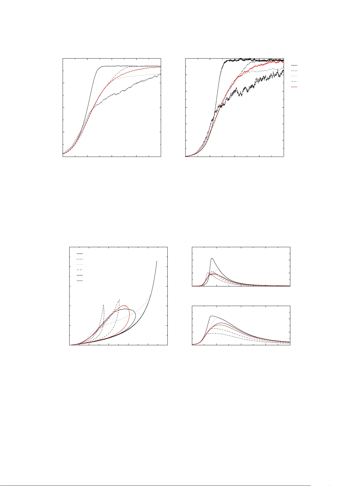
Comments & Academic Discussion
Loading comments...
Leave a Comment