M-decomposability, elliptical unimodal densities, and applications to clustering and kernel density estimation

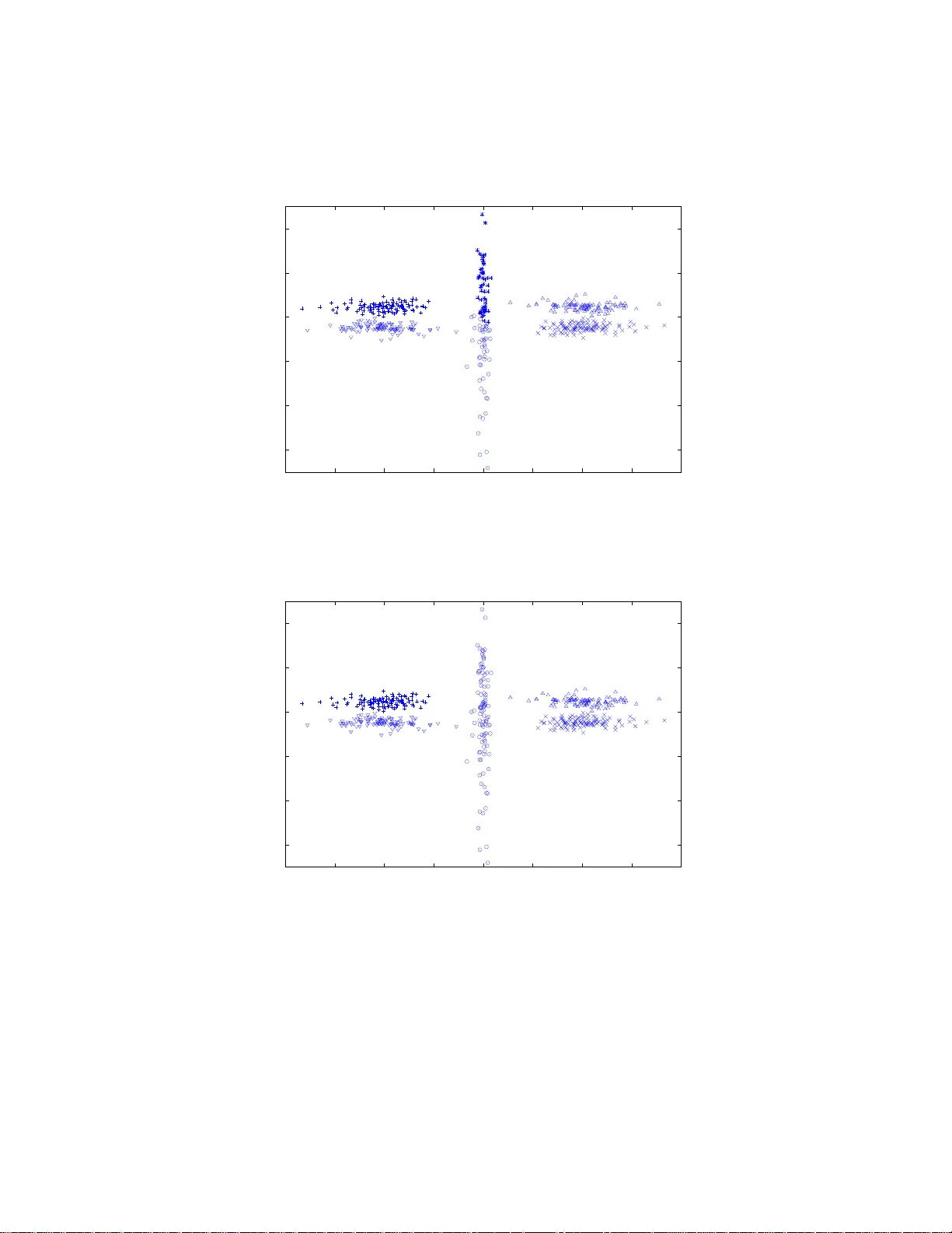
M -DECOMPOSABILITY, ELLIPTICAL UNIMOD AL DENSITIES, AND APPLI CA TIONS TO CLUSTERING AND KERNEL DENSITY ESTIMA TION NICHOLAS CHIA AND JUNJI NAKANO Abstract. Chia and Nak an o (2009) int ro duced the concept of M -decom- posabili t y of probab ility densities in one-dimension. In this pap er, we general- ize M -decomposability to any dimension. W e pro ve tha t all elliptical unimo dal densities are M -undecomposable. W e al so derive an inequality to show that i t is b etter to represent an M -decomp osable density via a mixture of unimodal densities. Finally , we demonstrate the application of M - decomposability to clustering and kernel density estimation, using real and simulated data. Our results sho w that M -decomposabili t y can be used as a non-parametric crite- rion to l ocate mo des i n probability densities. 1. Introduction In a recent paper , Chia and Nak ano (2009) conceptualiz ed M -decomp osa bilit y and develope d the theory in one - dimension. The main results are s umma r ized in the following parag raph. M -decomp osability is defined as follows. Let f b e a pr obability density defined in one-dimensio n. There exist co un tless wa ys to ex press f as a weigh ted mixture of tw o probability densities, in the form o f f ( x ) = α g ( x ) + (1 − α ) h ( x ) where 0 < α < 1 . If it is po ssible to find any combination of { α, g , h } , which satisfies σ f > σ g + σ h where σ f denotes the standard deviatio n of f , then the o riginal density f is said to b e M -de c omp osable . Otherwise, f is M - unde c omp osable . Int uitively , m ultimo dal dens ities with pea ks separated far apart are likely to b e M -decomp osable. Con versely , unimo dal densities ar e probably M - undecomp osable. The authors proved tha t all o ne-dimensional symmetric un imo dal densities with finite second momen ts are M -undecomp osable. In other words, if f is s ymmetric unimodal and has finite s econd momen ts, then for an y weighted mixture density comp onents { g , h } o f f , o ne must hav e (1.1) σ f ≤ σ g + σ h . Eq ( 1.1) applies to a wide range of densities that include Gaussian, Laplace, lo- gistic and many others. The authors also showed the po ssibility of using M - decomp osability to pe r form cluster analys is and mo de finding in one-dimension. 2000 Mathematics Subje ct Classific ation. Primary 62H30, 62G07; Secondary 15A45. Key wor ds and phr ases. cov ar iance matrices, inequalities, cluster analysis, elliptical unimodal densities, Kull bac k-Leibler divergence , density estimation, non-parametric criterion. 1 2 NICHOLAS CHIA AND JUNJI NAKANO Incident ally , the “ M ” in M -decomp osa bilit y ma y either mean “multimodal” or “mixture”. In this pap er, we further co n tribute to M -decomp osability , b oth in the theoret- ical and applica tional aspects. On the theor etical fr o n t, w e gener alize the concept of M -decomp osa bilit y to a n y d -dimensional s pace. First o f all, we der ive a theorem (Theorem 2.3) that is the d -dimensional equiv alent of Eq (1.1). W e prov e that all el liptic al u nimo dal densities with finite second moments are M -undecomp osa ble. These densities include mult iv aria te Gaussia n, Laplace, lo g istic and many others. F ollowing that, we derive another theor em, (Theo rem 2.4), which determines if a given densit y is b etter approximated via a mixture of Gaus s ian densities, instead of one s ingle Gaussia n density . One example of a pplication of M - undecompo sability is cluster ana lysis. F or decades, clus ter analysis has b een a p opular research sub ject, b oth from the theoret- ical and algo rithmic asp ects. Cluster analysis is likely to remain a widely r esearched topic, given the many different appro a ches that cater s to v a rying applications. The survey pap er by Berk hin (2002) pr ovides a n up-to-da te status of av ailable cluster - ing techniques a nd metho dologies. There are tw o main cla sses o f cluster analys is metho dologies: p ar ametric and non- p ar ametric . F or parametric cluster analy sis, one needs prior knowledge or ass umptions o n the analytical structure of the underly- ing clusters . The whole datase t is mo deled as a mixture o f k parametr ized densities, and the problem reduces to parameter e stimation. In McLachlan and Peel (200 0), parametric cluster analys is via the Exp e ctation-Maximization (E M) algor ithm is describ ed in detail. Other par ametric metho ds include the Bayesian particle fil- ter approach detailed in F earnhea d (2004), and the re v ersible jump Markov chain Monte Ca rlo (MCMC) a pproach b y Richardson and Green (1997). F or para metric cluster analysis , the mo s t p o pular approa c h is to mo del the clusters as Gaussia n densities. As for non-parametric cluster analysis, a p opular to ol is the k - means algo rithm. The k -means a lgorithm is optimal for lo c a ting similar - sized spherical cluster s within a dataset, provided the n umber of cluster s are known b eforehand. With elliptical clusters, o r clusters of v ary ing sizes, the k -mea ns approach yields results that a re meaningless. The k -mea ns algo rithm a ssigns samples to cluster s based on dis- tanc e (Euclidean o r its v ar iations) to the centres of the clusters. Other distanc e- b ase d non-par ametric cluster ing algo rithms include the nearest-ne ig h b our cluster- ing. Distance-ba s ed clustering a lgorithms ge ner ally s hare the sa me dr awbac ks such as sensitivity to sca ling , e lliptical cluster s and clusters o f v ar y ing sizes. If the nu m- ber of clusters a re not known b eforehand, neither the k -means algor ithm nor the nearest-neig h bo ur a lgorithm estimate the num b er of cluster s automa tically . F or the k - means algo rithm, the unknown num b er of cluster s has to b e re-ev aluated via Aka ike’s information criterion (AIC), prop osed by Ak aike (1974), or other suita ble mo del selection criterion. Our approach to cluster analy sis via M -decompo sability is non-parametric a nd are based on volume instead o f distance. Being non-para metric, prior k nowledge on the a nalytical struc tur e of the underlying clusters is unnecessary . The only as- sumption r equired is that the c lus ters are approximately elliptical and unimo dal. As a result, the limitation of clustering via M -undecomp osa bilit y is that it will probably not pe r form ideally for irregula rly shaped cluster s tha t devia te fro m el- liptical unimo dal densities. How ever, if the clusters are approximate elliptical and M -DECOMPOSABILITY 3 unimo dal, then o ur cluster ing metho dology works well, and allows for the unknown nu mber of cluster s to b e r ecov ered automatica lly . F ur thermore, a s clustering via M -decomp osability is ba s ed on volume instea d of distance, cluster allo catio n is inv aria n t to scaling. F or existing alter native metho dolog ies to clus ter ing, there ha s b e e n r ecent devel- opment on Rousseeuw’s minim um v olume ellipsoids (MVE) in Rousseeuw and Ler oy (1987) and Rousseeuw and v an Zo meren (1990). The MVE approach is originally developed a s a r obust metho d to estimate mean vectors and cov ariance matrices of multiv ariate da ta in the presence of outliers. MVE is computationa lly inten- sive and the optimal solution is often difficult to a c hieve, prompting many resea rch pap ers o n the a lgorithmic a sp e c ts o f the pro blem. Some authors, for ex ample, Shio da and T un¸ cel (2005), outlined a heur istic for c lus tering via MVE by min- imizing the sum of volume of clusters. Our metho dology of clustering v ia M - decomp osability has s ome similarities with cluster ing via the MVE appr oach, in that b oth measure “volume” in a certain sense . Central to the M - de c ompo sability concept is the “pseudo -volume”, which we define a s the square - ro ot of the determi- nant of the cov ar ia nce matrix. Co mpa red to MVE, the pseudo-volume is compu- tationally cheap and str aightforw ard. On top of that, we also provide theoretical justifications in Theorem 2.4 for minimizing the sum of pseudo-volumes o f clus ter s. Another p ossible area o f a pplica tion of M -undecomp osa bilit y is density esti- mation. In density estimation, data generated from some unknown densities a re given, and the task is to estimate and recov er the unkno wn densit y . One popular non-para metr ic approa ch to density estimation is kernel densit y estimation, treated in Silv erman (1 986), Sco tt (1 9 92), H¨ ardle et al (2004), as well as W a nd and Jones (1995). The difficulty in kernel density estimation is the der iv ation of the optimal kernel ba ndwidth: If the kernel bandwidth is underestimated, the kernel dens it y bec omes unduly spiky; if the kernel bandwidth is ov erestimated, the kernel density bec omes ov ersmo othed. F or multimoda l densities, it is not p ossible to find a s ing le kernel bandwidth that provides a satisfactory densit y estimation everywhere. Us- ing M -decomp osa bility , w e demonstrate that there is a simple and logical wa y to circumv en t the abov e problem by r epresenting the under ly ing density as a mixture of unimo dal densities whe r e nece s sary . This pap er develops b oth the theoretical and applicational asp ects of M - decom- po sability , a nd therefore should b e o f in terest to theor etical statisticians and practi- tioners alik e. Section 2 is devoted to the theoretical development of M -decomp osability in d -dimensional spa ce. F or reader s who a re only interested in applications, it is po ssible to note only the results of Theorems 2 .3 and 2.4, sk ipping the rest of Section 2 without disrupting the flow of the pap er. 2. M -Decomposability in d -Dimensional Sp ace 2.1. E xtensions from One-Di mension. In Chia and Nak ano (2009), M - decom- po sability inv olves o nly the sta ndard deviatio ns o f proba bility densities . This is bec ause in one-dimensio n, the sta ndard devia tion is a natur al mea sure o f scatter of a given densit y . The standard devia tio n of any density in o ne-dimension has the same order as the distance or “length” computed from the mean. When co nsidering higher dimensions, a p ossible co rresp onding measure of sca tter of a given densit y is the squar e-ro ot of the deter minant o f the cov aria nce matrix of the density . The square-r o ot of the determinant of the cov aria nce matrix in d -dimensiona l space 4 NICHOLAS CHIA AND JUNJI NAKANO has the same or der as d -dimensio nal “ h yp ervolume”. Henceforth, w e shall call the ab ov e mea sure the pseudo-volume of a density . W e denote the cov ariance matr ix of a density f by Σ f , a nd therefore the pseudo-volume of f is given by | Σ f | 1 2 . In one-dimension, pseudo- volume reduce s to the sta ndard deviatio n. In Chia and Nak a no (200 9), the authors limited the n um ber of mixture compo - nent s to tw o in their developmen t of M - decomp osability . In this pap er, we show that it is p os s ible to relax the above limitatio n, and g eneralize the num ber of mix- ture compo nen ts to m w he r e m ≥ 2. Let f b e a proba bilit y density function defined on R d , the d -dimensiona l r e al space. One can alw ays expres s f as a weigh ted mix- ture of m dens ities as follo ws: (2.1) f ( x ) = α 1 g 1 ( x ) + · · · + α m g m ( x ) , where 0 < α i < 1 a nd Σ α i = 1 . Henceforth, we call an y set of densities { g 1 , . . . , g m } which satisfies Eq (2.1) a set of mixtur e c omp onents of f . W e extend the definition of M -decomp osability to d -dimensional space as follows. Definition 2.1 ( M -Decomp osa bilit y) . F or a given pr ob ability density function f , if ther e exists a set of mixtur e c omp onents { g 1 , . . . , g m } such that | Σ f | 1 2 > | Σ g 1 | 1 2 + . . . + | Σ g m | 1 2 , then f is define d to b e M -de c omp osable. Ot herwise, f is M -u nde c omp osable. If for any set of mixt ur e c omp onents { g 1 , . . . , g m } , | Σ f | 1 2 < | Σ g 1 | 1 2 + . . . + | Σ g m | 1 2 , then f is strictly M -u nde c omp osable. Our new definition o f M - de c o mpo sability r educes to that pres en ted in Chia a nd Nak ano (2009) when m = 2 a nd d = 1. F or d ≥ 2, the definition o f M -deco mpo s ability can be describ ed compactly using pseudo-volumes. 2.2. E lliptical Uniform Densities . The uniform density is triv ially defined in one-dimension, but in higher dimensions , it may assume ma n y differ en t p ossible shap es. F or example, one may think of the uniform hyperc ube o r the uniform hypersphere. How ever, the sub ject of interest in our pap er is the el liptic al uniform density , which forms the fundamen tal building blo ck of elliptical unimo dal densities. Ellipticity , unifor mit y and unimo dality a r e thre e differen t qua lities. The defini- tions of the first tw o are given immediately b elow, and the third will b e g iven in Section 2.3. Definition 2 .2 (Elliptical and Spherical Densities) . We say that f is elliptica l if ther e exist a ve ctor µ ∈ R d , a p ositive semidefinite symmetric matrix Σ ∈ R d × d and a p ositive function p on R + ∪ { 0 } such that f ( x ) = p { ( x − µ ) T Σ − 1 ( x − µ ) } . F ur t hermor e, if Σ = k I d , wher e k > 0 and I d denotes the d -dimensional identity matrix, then f b e c omes f ( x ) = p 1 { ( x − µ ) T ( x − µ ) } = p 2 ( | x − µ | ) , and we say t hat f is spherical . M -DECOMPOSABILITY 5 Remark The mean and cov a riance matrix of the ab ov e- defined elliptical dens it y f a re as follows: µ f = µ, Σ f = c Σ wher e c > 0 . Definition 2.3 (Uniform Densities) . We say that f is elliptical unifor m if ther e exist a ve ctor µ ∈ R d , a p ositive semidefinite symmetric m atrix Σ ∈ R d × d , and a p ositive r e al numb er r such that f ( x ) ∝ I ( x − µ ) T Σ − 1 ( x − µ ) 0 and I d denotes the d -dimensional identity matrix, then f b e c omes f ( x ) ∝ I ( x − µ ) T ( x − µ ) | Σ u | 1 2 . Without los s of generality , set ma x( u ) = M and therefo re | Σ u | 1 2 = Γ( d 2 + 1) M { π ( d + 2) } d 2 . Rewriting the elliptical uniform densit y u as mix ture comp onents, we have u ( x ) = α 1 v 1 ( x ) + . . . + α m v m ( x ) for so me { α 1 , . . . , α m } satisfying 0 ≤ α j ≤ 1 a nd Σ α j = 1 . As a result, we have v j ( x ) ≤ u ( x ) α j ≤ M α j for all 1 ≤ j ≤ m . Using L e mma 2.1, we hav e (2.2) | Σ v j | 1 2 ≥ α j Γ( d 2 + 1) M { π ( d + 2) } d 2 = α j | Σ u | 1 2 6 NICHOLAS CHIA AND JUNJI NAKANO for all j , with equalities holding if and only if the density in question is elliptical uniform. Now, for d > 1, we can hav e at most ( m − 1) but never al l of v ’s to b e elliptical uniform satisfying Eq (2.2). Therefor e, | Σ v 1 | 1 2 + . . . + | Σ v m | 1 2 ≥ | Σ u | 1 2 . Ident ity may only ho ld when d = 1, refer to Chia and Nak ano (2009).  2.3. E lliptical Unimo dal Densiti es. In one-dimension, sy mmetry is trivial to visualize and expres s mathema tically . In higher dimensions , symmetr y ma y b e de- picted via ellipticity . As such, el liptic al unimo dal densities play a key role in this pap er. W e pr ovide a definition for elliptical unimo dal densities b elow. E lliptical densities in g eneral have b een treated in detail by many resear chers, see F ang et al (1990) and refer ences within. Unimo dal densities ha v e also be e n the sub ject o f ac- tive resear ch. F or example, r e fer to Anderso n (1955), Dharmadhik ari and Joag-Dev (1987) as w ell as Ibr a gimov (1956). Definition 2. 4 (E lliptical Unimo dal Densities ) . We say that f is elliptica l uni- mo dal if ther e exist a ve ctor µ ∈ R d , a p ositive semidefinite symmetric matrix Σ ∈ R d × d and a non-increasing p ositive fu n ction p on R + ∪ { 0 } such that f ( x ) = p { ( x − µ ) T Σ − 1 ( x − µ ) } . Comparing with Definition 2.2, the only additiona l info r mation in Definition 2 .4 is that the positive function p ha s to be non-increasing as well. According to Defi- nition 2.4, elliptical unimo dal densities ar e tho s e whose cr oss-sectio ns a r e elliptical, and with mean ( µ ) a nd cov arianc e matrices pr opo rtional to (Σ). D efinition 2.4 encompasses a large class of general densities including d -dimensional elliptical uni- form, Gaussia n, logistic, Lapla ce, V on Mises, b eta( k , k ) where k > 1, student- t , and many other densities . Henceforth, we prop ose the following alter native r epresentation of elliptical uni- mo dal densities. Theorem 2. 2 (Representation of Elliptica l Unimoda l Densities) . Le t f b e an el lip- tic al un imo dal density with me an µ and c ovaria nc e matrix Σ . Then, for al l ǫ > 0 , it is p ossible to c onstruct a density g n ( x ) = n X j =1 b j u j ( x ) such that Z | g n ( x ) − f ( x ) | d x < ǫ . Her e, e ach u j is an elliptic al u n iform density su ch that (2.3) u j ( x ) ∝ I ( x − µ ) T Σ − 1 ( x − µ ) 0 , b j = m X i =1 c i,j > 0 . 8 NICHOLAS CHIA AND JUNJI NAKANO If c i,j > 0 for a pair of ( i, j ), then v i,j ( x ) is a density . F ro m Eq (2.6), we can r ewrite each elliptical uniform u j as u j ( x ) = m X i =1 c i,j b j v i,j ( x ) . F ollowing the argument pres en ted in Theor em 2.1, w e ha ve | Σ v i,j | 1 2 ≥ c i,j b j | Σ u j | 1 2 , with eq ualit y ho lding if a nd o nly if v i,j is elliptical uniform having “thickness” satisfying max { c i,j v i,j ( x ) } = max { b j u j ( x ) } . Similarly , rewriting ea ch mixture component g i in terms of v i,j , we obtain g i ( x ) = n X j =1 c i,j a i v i,j ( x ) ≡ n X j =1 s i,j v i,j ( x ) . Next, we create new spheric al unimo dal densities ˜ g i ’s corres p onding to each g i to facilitate lo wer b oundings o f | Σ g i | . Define ˜ g i as follows: ˜ g i ( x ) = n X j =1 c i,j a i ˜ v i,j ( x ) ≡ n X j =1 s i,j ˜ v i,j ( x ) . In the ab ove, each { ˜ v i, 1 , . . . , ˜ v i,n } are spheric al uniforms whose means co inc ide and such that max { c i,j ˜ v i,j ( x ) } = max { b j u j ( x ) } for all { i, j } , hence y ie lding | Σ ˜ v i,j | 1 2 = c i,j b j | Σ u j | 1 2 . Computing the determinan t of the cov ar iance matrix o f g i , we hav e | Σ g i | = | ( s i, 1 Σ v i, 1 + · · · + s i,n Σ v i,n ) + ( s i, 1 µ v i, 1 µ T v i, 1 + · · · + s i,n µ v i,n µ T v i,n ) | ≥ | s i, 1 Σ v i, 1 + · · · + s i,n Σ v i,n | ≥ ( s i, 1 | Σ v i, 1 | 1 d + · · · + s i,n | Σ v i,n | 1 d ) d ≥ ( s i, 1 | Σ ˜ v i, 1 | 1 d + · · · + s i,n | Σ ˜ v i,n | 1 d ) d = | s i, 1 Σ ˜ v i, 1 + · · · + s i,n Σ ˜ v i,n | = | Σ ˜ g i | . The first inequalit y holds as a res ult of (2.7) | K 1 + K 2 | ≥ | K 1 | , where K 1 and K 2 are b oth non-neg ative definite s ymmetric d × d matrices. The second inequa lit y holds because (2.8) | K 1 + K 2 | 1 d ≥ | K 1 | 1 d + | K 2 | 1 d , with identit y holding if and only if K 1 and K 2 are pr op ortional. The pro of o f b oth Eqs (2 .7) a nd (2.8) c a n b e found in Cov er and Thomas (1988). The third inequality holds as w e must have | Σ v i,j | ≥ | Σ ˜ v i,j | M -DECOMPOSABILITY 9 as a direct result of Lemma 2.1. The equality that follows the third inequality is again a result o f Eq (2.8), as all Σ ˜ v i,j ’s ar e prop or tio nal to the identit y ma trix. W e hav e just sho wn that | Σ g i | ≥ | Σ ˜ g i | for all g i , i.e. the pseudo-volume of ea ch g i is minimized when g i is spherical unimo dal. Therefore, a sufficien t condition to (Claim 1) is (Claim 2) | Σ f | 1 2 ≤ | Σ ˜ g 1 | 1 2 + . . . + | Σ ˜ g m | 1 2 . Since f is elliptical unimo dal, it is p oss ible to find a corr esp onding spherica l unimo dal density f s such that the hypervolumes are preserved, i.e. | f s | = | f | . T o prov e (Claim 2 ), we only have to deal with the pseudo-volumes of spher ical unimo dal densities. W e obtain | Σ ˜ g i | a s follo ws | Σ ˜ g i | = 1 ( d + 2 ) d · ( c 1+ 2 d i, 1 + · · · + c 1+ 2 d i,n c i, 1 + · · · + c i,n ) d . Here, w e make use of the fact that the cov ar iance of a d -dimensional spherical uniform density defined b y u ( x ) ∝ I | x − µ | 0 . Then the fol lowing ine quality holds for any p ositive inte gers d and n . ( a 1+ 2 d 1 + · · · + a 1+ 2 d n a 1 + · · · + a n ) d 2 ≤ ( b 1+ 2 d 1 + · · · + b 1+ 2 d n b 1 + · · · + b n ) d 2 + ( c 1+ 2 d 1 + · · · + c 1+ 2 d n c 1 + · · · + c n ) d 2 . Equality hold s if and only if the se quenc es a i , b i and c i ar e line arly dep endent. Pr o of. T he pr o of is similar to that o f Chia and Nak ano (2009), with the only difference b eing in d . W e pr o c e e d in the spir it of Hardy et al (1988), as well as P ` o lya and Szeg ¨ o (19 72). Set x ≡ [ x 1 , · · · , x n ] T , y ≡ [ y 1 , · · · , y n ] T and z ≡ 10 NICHOLAS CHIA AND JUNJI NAK ANO [ z 1 , · · · , z n ] T and simila rly for a , b , c . Let x = t y + (1 − t ) z , i.e. x i = t y i + (1 − t ) z i for all i . F urthermore, define the function f as fo llows: f ( x ) = ( x 1+ 2 d 1 + · · · + x 1+ 2 d n x 1 + · · · + x n ) d 2 , and set φ ( t ) = f { t y + (1 − t ) z } ≡ f ( x ) , where 0 ≤ t ≤ 1. It suffices to prove that φ ′′ ( t ) ≥ 0 for 0 ≤ t ≤ 1 . This is an immediate conseque nc e of Jensen’s inequalit y as φ ′′ ( t ) ≥ 0 implies φ ( t ) ≤ t φ (0) + (1 − t ) φ (1) . Setting t = 1 2 , we hav e f ( y 2 + z 2 ) ≤ 1 2 f ( y ) + 1 2 f ( z ) . Denoting by y = b , z = c , this b ecomes f ( a 2 ) ≤ 1 2 f ( b ) + 1 2 f ( c ) . How ever, fro m the definition of f , w e m ust hav e f ( a 2 ) = 1 2 f ( a ) . Therefore φ ′′ ( t ) ≥ 0 implies f ( a ) ≤ f ( b ) + f ( c ) a s required. E quality holds if and only if φ ′′ ( t ) = 0. W e shall b egin from the definition of φ a s follows: φ ( t ) = f ( x ) = (Σ x 1+ 2 d i ) d 2 (Σ x j ) − d 2 . Different iating φ t wice with respec t to t and rearra nging, we hav e φ ′′ ( t ) φ ( t ) = d ( d + 2) 4 · { Σ( y k − z k ) Σ x j − Σ x 2 d k ( y k − z k ) Σ x 1+ 2 d i } 2 | {z } A + ( d + 2 d ) · (Σ x 1+ 2 d i ) − 2 · [ (Σ x 1+ 2 d i ) · { Σ x 2 d − 1 j ( y j − z j ) 2 } − { Σ x 2 d k ( y k − z k ) } 2 ] | {z } B . The term A is express ible as a squa re and therefor e greater or equa l to 0. T o ev aluate B , we set p 2 i = x 1+ 2 d i and q 2 j = x 2 d − 1 j ( y j − z j ) 2 , yielding B = (Σ p 2 i ) · (Σ q 2 j ) − (Σ p k q k ) 2 ≥ 0 via Cauchy-Sc hwarz’s inequa lit y . Therefore w e m ust have φ ′′ ( t ) ≥ 0 due to the non-negativeness of x i , y i and z i . Hence, Lemma 2.2, and consequen tly , Theorem 2.3 is prov ed.  As a res ult of Theor e m 2.3, all elliptical unimo dal densities with finite s e cond mo- men ts are M -undecomp osable. Conv ersely , any density , which is M -decomp osable, cannot b e elliptica l unimoda l. One can do b etter tha n that. In the next subsection, we fur ther show that if f is M -dec ompo sable, then there exists a n approximation to represent f via a mixture of Gaus sian densities, which improv es estimatio n o f f . M -DECOMPOSABILITY 11 2.5. E stimation of M -Decomp osable Densitie s. Theorem 2.4 (Inequality on M - Deco mpo s able Densities) . L et f b e pr ob abili ty density funct ions define d on x ∈ R d . L et { g 1 , . . . , g m } b e a set of mixt ur e c omp o- nents of f such that f ( x ) = α 1 g 1 ( x ) + . . . + α m g m ( x ) , wher e 0 < α j < 1 and Σ α j = 1 . Then the fol lowing r esult app lies: | Σ f | 1 2 > | Σ g 1 | 1 2 + . . . + | Σ g m | 1 2 ⇒ K L ( f k ˜ f ) > K L ( f k α 1 ˜ g 1 + . . . + α m ˜ g m ) . Her e, K L ( p k q ) denotes the Kul lb ack-L eibler diver genc e b etwe en densities p and q , given as K L ( p k q ) = Z p ( x ) log p ( x ) q ( x ) d x . F ur t hermor e, ˜ f denotes t he Gauss ian density whose me an and c ovarianc e matrix c oincide with those of f , and ˜ g ’s ar e similarly define d. Pr o of. W e o nly need to pr ov e that (Claim A) Z f ( x ) lo g ˜ f ( x ) d x < Z f ( x ) lo g { α 1 ˜ g 1 ( x ) + . . . + α m ˜ g m ( x ) } d x . Now, RHS of (Claim A) = Z { α 1 g 1 ( x ) + . . . + α m g m ( x ) } · log { α 1 ˜ g 1 ( x ) + . . . + α m ˜ g m ( x ) } d x ≥ α 1 Z g 1 ( x ) lo g { α 1 ˜ g 1 ( x ) } d x + . . . + α m Z g m ( x ) log { α m ˜ g m ( x ) } d x = α 1 { log α 1 + Z g 1 ( x ) log ˜ g 1 ( x ) d x } + . . . + α m { log α m + Z g m ( x ) log ˜ g m ( x ) d x } . F rom definitions, the pr obabilitiy density function o f ˜ g ( x ) is given by ˜ g ( x ) = (2 π ) − d 2 | Σ g | − 1 2 exp {− 1 2 ( x − µ g ) T Σ − 1 g ( x − µ g ) } , where µ g and Σ g denote the mean and cov ar iance matrix of g . W e obtain Z g ( x ) lo g ˜ g ( x ) d x = − d 2 log(2 π ) − 1 2 log | Σ g | − d 2 . Hence, RHS of (Claim A) ≥ α 1 { log α 1 − 1 2 log | Σ g 1 | } + . . . + α m { log α m − 1 2 log | Σ g m | } − d 2 log(2 π ) − d 2 . Meanwhile, LHS of (Claim A) = − d 2 log(2 π ) − 1 2 log | Σ f | − d 2 . T o co mplete the pr ov e o f Theor em 2.4, it suffices to demo ns trate that (Claim B) α 1 log | Σ g 1 | 1 2 α 1 + . . . + α m log | Σ g m | 1 2 α m < lo g | Σ f | 1 2 . 12 NICHOLAS CHIA AND JUNJI NAK ANO -60 -40 -20 0 20 40 -80 -60 -40 -20 0 20 40 60 80 original data Figure 1. Or iginal data from mult imo dal density drawn from mixture of five log istic densities. Using Jensen’s inequalit y , we hav e LHS of (Claim B) ≤ log( α 1 | Σ g 1 | 1 2 α 1 + . . . + α m | Σ g m | 1 2 α m ) = lo g( | Σ g 1 | 1 2 + . . . + | Σ g m | 1 2 ) < lo g | Σ f | 1 2 = RHS of (Claim B) , which completes the pro of of Theorem 2.4  W e s ummarize the result o f Theorem 2.4 as follows. Le t f be any density in d -dimensional spac e. If f is M -decomp osa ble, then by definition, o ne can find a set o f mixture comp onents of f , such tha t the sum of ps eudo-volumes of the mixture comp onents is less than the pseudo-volume of the origina l density f . F rom Theorem 2.3, f cannot b elong to the class of elliptical unimo dal densities. It is po ssible to do b etter than that. Theo rem 2.4 shows that f is b etter estimated via a weigh ted Gauss ian mixture, ra ther than a single Ga us sian density . The Gaussian comp onents are cr eated via moments matching of the mixture comp onents of f . The b etter go o dness o f fit by the r e sultant weigh ted Ga ussian mixture es timate is guara n teed in Kullba c k-Leibler sense. It should b e noted that the a na lytical form o f the original density f do es not need to b e known. In the next section, we demonstra te the us e of Theo rems 2.3 and 2.4 to satistica l applications, namely cluster ana lysis and kernel density estimation. 3. Applica tions Using M -Decomposability 3.1. C l ustering via M -Decom p osability: The P o wer of Two. One straight- forward application of M -decomp osability is cluster analysis. Many existing clus- tering algorithm divide the dataset in to clusters, based on the following heur istic: That the within-v aria nc e s of cluster s are minimized while the b et ween-v a riance is M -DECOMPOSABILITY 13 -60 -40 -20 0 20 40 -80 -60 -40 -20 0 20 40 60 80 first decomposition Figure 2. Origina l data split into tw o mix tur e co mp onents, rep- resented by tw o differe n t sym bols . The sum of pseudo-volumes of the mixture comp onents is less than that of or ig inal. maximized at the same time. Another v ariation to this heuristic is to deter mine cluster allo cations s uc h that a function of volume of clusters is minimized. In partic- ular, Shio da and T un¸ cel (2 005) prop osed dividing the dataset into k clusters, suc h that the total sum of MVE (minim um volume o f ellipso id) of k clusters are globally minimized. While the details for each a lgorithm may differ, the underlying idea is conceptually similar. Theor em 2.4 pro vides theoretical justification for minimizing sum of pseudo-volumes, and ther efore supp orts all simila r approaches of existing algorithms. Int uitively , the rigo rous appro ach to implement cluster a nalysis v ia Theorem 2.4 is to divide the dataset into k ( ≥ 1) clusters, such that the sum of pseudo-v olumes of a ll cluster s a re globally minimized. This appr oach is co mputationally unfeas ible for dataset of a n y r easonable size. T o this end, we prop ose the following alternative approach that captures the essence o f Theor em 2 .4 as far a s p ossible. W e devise a split-merge clustering str ategy that inv o lves splitting and merging, tw o clus ters at a time. This low ers the overall computationa l loa d. W e show tha t with our approach, the algorithm is able to overcome lo cal minima. Consequently , it is po ssible to p erfo rm cluster analysis well, even with k ( > 2) clusters. F rom the given sa mple F = { X 1 , · · · , X n } , we are int erested to know if the original sa mple is M -deco mpos a ble. W e chec k if F can be partitio ned int o tw o clusters, such that the sum of pseudo-volumes of the clusters is less than that of F . W e denote a s { G, H } , a par tition of F , such that G = { Y 1 , · · · , Y m } , H = { Y m +1 , · · · , Y n } and G ∪ H = F , with Y ’s b eing a rear rangement of X . W e further denote the sample cov ar ia nce ma tr ices of F, G, H as S F , S G and S H . Our task is to find the 14 NICHOLAS CHIA AND JUNJI NAK ANO -10 0 10 20 30 40 0 10 20 30 40 50 60 70 sub-decomposition of cluster labeled (+) in Fig 2 Figure 3. Mixture component denoted by (+) in Fig 2 split in to t wo further mixture comp onents. -60 -50 -40 -30 -20 -10 0 10 -70 -60 -50 -40 -30 -20 -10 0 sub-decomposition of cluster labeled (o) in Fig 2 Figure 4. Mixture comp onent denoted by (o) in Fig 2 split in to t wo further mixture comp onents. optimal par titio n { G, H } suc h that |S G | 1 2 + |S H | 1 2 is globa lly minimized and test this v a lue against |S F | 1 2 . If (3.1) |S G | 1 2 + |S H | 1 2 |S F | 1 2 < 1 + τ s , M -DECOMPOSABILITY 15 -10 -5 0 5 10 10 20 30 40 50 60 70 sub-decomposition of cluster labeled (+) in Fig 3 Figure 5. Mixture component denoted by (+) in Fig 3 split in to t wo further mixture comp onents. -10 -5 0 5 10 -70 -60 -50 -40 -30 -20 -10 sub-decomposition of cluster labeled (o) in Fig 4 Figure 6. Mixture comp onent denoted by (o) in Fig 4 split in to t wo further mixture comp onents. where τ s is a threshold v alue clos e to zero , then, we can conclude that F is likely to be M -decomp osable. How ever, if E q (3.1) is not satisfied, then F is likely to b e M - undecomp osable. T o robustify the “splitting pro cess” against lo cal minima traps, it is p ossible to s e t the RHS of Eq (3.1) to b e greater tha n 1. F urthermore, tak ing int o considera tion er ror due to finiteness of sa mple sizes, impe rfection of splitting 16 NICHOLAS CHIA AND JUNJI NAK ANO algorithms, and als o acco un ting fo r limiting the num ber of mixture comp onents to t wo, we recommend that the τ s on the RHS of E q (3.1) to be ab out 0 . 05 . When one co ncludes that a particular cluster F is probably M - undecom-p osable, it is p ossible to stop at o ne cluster . How ever, if F is found to be M - decompo sable int o clusters of G a nd H , one may rep eat the splitting pro cess for G and H . The pro cess is then reitera ted until all cluster s are pr obably M -undecomp osable. When that happ ens, the splitting pr o cess ends. Our str ategy also includes “merging” of clusters. At the p oint when a ll splitted clusters are probably M -undeco mpos a ble, we select tw o clusters at a time and per form the following test. Now, let Q, R denote the tw o chosen cluster s a nd P be the union of the tw o clusters, i.e. P = Q ∪ R . W e then chec k the s um of the pseudo-volumes o f Q and R and compare against that of P . If (3.2) |S Q | 1 2 + |S R | 1 2 |S P | 1 2 ≥ 1 + τ m , we conclude that Q and R sho uld b e merg ed to form a larg er clus ter P . This pro cess is r epea ted un til there are no mor e mergeable clusters left. T o preven t ov erclustering, we recommend τ m to b e a round − 0 . 05. W e hav e descr ibed a p oss ible algor ithm using M -decomp osa bilit y to p erform cluster analysis. The crucial p oint is to find a partition { G, H } such that |S G | 1 2 + |S H | 1 2 is minimized as far as possible. Ther e are ma n y p ossible approaches to this task. T o find the global minim um of the sum |S G | 1 2 + |S H | 1 2 is c o mputationally unfeasible and may be NP-har d. Her e, we propo se a computationally simpler ap- proach. At each spitting step, we simply fit a tw o-mixture Gaussian to the origina l cluster F , and then run the EM algo rithm to con vergence to obtain the par tition { G, H } . How ev er, we emphasize that the EM algor ithm approa ch itself is not criti- cal, and that it is p ossible to use other approa ches to o btain a r easonable par tition { G, H } of F a t the splitting step. The main p oint here is the concept o f cluster- ing via M -decomp osa bilit y . In the tw o examples pr esented b elow, we show that it is p ossible to p erfor m clus tering a nalysis reaso nably well, using o ur prop osed algorithm. 3.2. C l ustering of Simulated Data. The simulation ex ample provided her e is drawn from a fiv e-mixture logistic densities as follows. The s a mple F is generated b y 100 samples each fro m five logistic densities with the following means and cov ariance matrices: L 1 :  − 40 5  ,  12 π 2 0 0 π 2 3  L 2 :  − 40 − 5  ,  12 π 2 0 0 π 2 3  L 3 :  0 0  ,  π 2 3 0 0 48 π 2  L 4 :  40 5  ,  12 π 2 0 0 π 2 3  L 5 :  40 − 5  ,  12 π 2 0 0 π 2 3  M -DECOMPOSABILITY 17 -60 -40 -20 0 20 40 -80 -60 -40 -20 0 20 40 60 80 all 6 sub-clusters Figure 7. All s ix M -undecomp osable clusters of orig ina l data, represented by six differen t symbols. -60 -40 -20 0 20 40 -80 -60 -40 -20 0 20 40 60 80 final cluster allocation: 5 clusters Figure 8. Final cluster allo cation for med by merging clus ters from Fig 7. Five clusters are recovered faithfully . Fig 1 sho ws the original sample F . Clustering is p erformed without knowledge o f either the num b er of clus ter s or the functional form o f the clusters. At the fir st split step, we fit a t w o-Gassia n mixture to F , and p erform EM to o btain the partition { G, H } . The result is shown in Fig 2. As Eq (3.1) is satisfie d for F, G, H , we split F int o G and H . This is a cas e o f EM co nverging to a local minima as it is (visually) unlikely that G and H are meaningful clusters of F . How ever, from Eq (3.1), it 18 NICHOLAS CHIA AND JUNJI NAK ANO -60 -40 -20 0 20 40 -80 -60 -40 -20 0 20 40 60 80 k-means: 5 clusters Figure 9 . Final c lus ter allo ca tion via k -means , represented by five differ en t symbols. k -means algorithm fails to recov er cluster s faithfully . is theoretica lly b etter off to split F in to G a nd H . The theoretical justification is given in Kullback-Leibler sense. The splitting pro cess is rep eated for G and H and the r esults a re shown in Figs 3 and 4. The splitting pro cess c ont inues until we arrive at six cluster s that are ar e all M -undecomp osable (Fig 7 ). Finally , we b egin the merg ing pro cess and find that the t w o clusters Q , sho wn as asterix (*) and R , shown as circle (o) in Fig 7 , satisfy Eq (3.1) where P = Q ∪ R . The tw o clusters are then merg ed a nd we are left with five cluster s shown in Fig 8. This example shows that our algor ithm is easy to implement and is robust to lo cal minima. A p opular clustering a lgorithm is the k -means metho d, which is o ptimal for nearly spheric a l clusters. How ev er, it do es not work here b ecause of the presence of inher en tly elongated clusters . Even by setting k = 5, the k -means method does not achieve a meaning ful cluster allo cation, as shown in Fig 9. Cluster a nalysis via k -means is sensitive to resca ling of axes, b ecause k -means inv olves comparison of distances. T o improv e the p e r formance o f k -mea ns analysis , there exist ma ny pre- pro cessing heuristics, e.g. rescaling the ax e s such that all axial units or ma rginal standard deviations b ecome compa tible. F or this simulation example, resca ling is unlikely to improv e cluster a nalysis via k -means b ecause elongated cluster s are not likely to b e eliminated. On the other ha nd, clus ter analysis via M - de c o mpo sability inv o lves comparison of pseudo-volumes instead of dista nces, a nd are there fore in- variant to rescaling of a xes. 3.3. C l ustering of Iris Dataset. Next, we analyze Fisher’s Iris datase t via M - decomp osability . The dataset was obtained from Asuncion and Newman (2 007). The da taset consists of 1 5 0 four-dimensiona l data. The four attribute information given a r e s epal length, sepa l width, p etal length a nd p etal width, all in centimetres. There ar e a ltogether three classes, namely “Setosa”, “V er sicolor” and “ Virginica”, in the propor tion of 50 : 50 : 50. M -DECOMPOSABILITY 19 2 2.5 3 3.5 4 4.5 5 5.5 6 6.5 7 7.5 2nd component: sepal width 1st component: sepal length 2 2.5 3 3.5 4 1 2 3 4 5 6 2nd component: sepal width 3rd component: petal length 0.5 1 1.5 2 2.5 4.5 5 5.5 6 6.5 7 7.5 4th component: petal width 1st component: sepal length 0.5 1 1.5 2 2.5 1 2 3 4 5 6 4th component: petal width 3rd component: petal length Figure 10. T rue Iris data: setosa(as ter ix), versicolor (cross), virg inica(triangle). W e p erform cluster analysis of the dataset via M -decomp osa bility , without knowledge of the actual num b er of classes. At the end of the analysis, we co n- firm that there are altogether three cla sses, in the prop ortion of 50 : 4 5 : 55 . The first 50 data coinc ide with “Setosa” (0 missp ecification). F or “V ers icolor” and “Virginica” , there are alto gether five missp ecifications. (Five “V er sicolor” a re mis- lab eled as “Virginica” ). The data is depicted gr aphically in Fig 10 (true class) a nd Fig 11 (estimated class). Although our analysis results in five cases of missp ecifications, our allo cation of “V er sicolor” and “ Virginica” achieves a sma ller pseudo-volume than the “true class”. Denoting the “true” classification of “V ersicolo r” and “ Virginica” b y { v 1 , v 2 } , and our estimation by { ˆ v 1 , ˆ v 2 } res p ectively , our estimation yields | Σ ˆ v 1 | 1 2 + | Σ ˆ v 2 | 1 2 ≈ 0 . 01563 , as compa red to | Σ v 1 | 1 2 + | Σ v 2 | 1 2 ≈ 0 . 01587 . The pseudo-volume of “ V ersicolo r” and “Virginica” co m bined into a single cla ss is approximately 0 . 01 799. 20 NICHOLAS CHIA AND JUNJI NAK ANO 2 2.5 3 3.5 4 4.5 5 5.5 6 6.5 7 7.5 2nd component: sepal width 1st component: sepal length 2 2.5 3 3.5 4 1 2 3 4 5 6 2nd component: sepal width 3rd component: petal length 0.5 1 1.5 2 2.5 4.5 5 5.5 6 6.5 7 7.5 4th component: petal width 1st component: sepal length 0.5 1 1.5 2 2.5 1 2 3 4 5 6 4th component: petal width 3rd component: petal length Figure 11. Iris da ta recov ered via M -decomp osability: se- tosa(aster ix ), versicolor(cros s), v ir ginica(triangle ). 3.4. K ernel De nsit y Estimation. Density estimation is an imp ortant statistical to ol that is widely used in man y scien tific and eng ine e ring fields. Given ra w mea - surements or da ta, the task is to r ecov er the unknown density from which the or ig- inal data is genera ted. The problem sta temen t is as follows. Given { X 1 , · · · X n } , which is gener ated from an unknown distribution with dens it y f , the task is to estimate f . F o r simplicity , we consider only univ a riate density estimatio n. In dens it y estimation, it is usually difficult y to deter mine qua n titatively the nu mber of modes in the underlying distribution, just from the g iv en data. In this resp ect, Theor em 2.4 can b e used for parametr ic density es tima tio n via Ga us s- ian mixtures. Besides via Ga ussian mixtures, a p opular a pproach to density es - timation is via the kernel density estimator . The kernel density estimator ap- proach is non-parametr ic and is treated in detail in Scott (19 9 2), Silverman (1986), W and and Jones (1995), H¨ ar dle et al (2004). The formula for the kernel density estimator, given data { X 1 , · · · X n } is (3.3) ˆ f ( x ; b ) = ( nb ) − 1 n X i =1 K { ( x − X i ) /b } , see, e.g. W and and Jones (1995). Usua lly K is chosen to b e a unimo dal density that is symmetric ab out zero, and is calle d the kernel . The p ositive num b er b is called the b andwidth . Such a for m ulation ensures that ˆ f ( x ; b ) is a lso a density . One pro per ty of the kernel density estimator is that the c hoice bandwidth is mor e impo rtant tha n the choice of the kernel itself. The optimal choice of the ba ndwidth ensures tha t the densit y estimate b ecomes optimally smo othed. One p opular choice of the bandwidth is (3.4) b = n − 1 5 ˆ σ , M -DECOMPOSABILITY 21 where ˆ σ is the sample standard devia tio n of the given data a nd n denotes the sample size. One known problem of the ba ndwidth given in Eq (3.4) is that it works well for densities that are appr oximately symmetric unimo dal. F or multimodal densities, the bandwidth tends pro duce an oversmoo thed density . Here, we prop ose an M -decomp osa bilit y based alg orithm to impr ov e kernel den- sity estimation. As we are only dea ling with the univ aria te case, w e consider just the sorted data F = { X [1] , · · · X [ n ] } . Similar to Section 3.1, we p erform clustering of F via splitting a nd merging. In one-dimension, the splitting pro cess b ecomes m uch s impler as we just hav e to find m (2 < m < n − 1) such that ( σ G + σ H ) is minimized. F or clarit y of expla nation, we assume that the orig inal data F has t wo clusters , and that G = { X [1] , · · · X [ m ] } and H = { X [ m +1] , · · · X [ n ] } ar e the optima l pa r tition of F . W e also have σ G + σ H < σ F . As s uch, we can ex pect the density estimation via the weigh ted mixture of G and H to b e b etter than that of the origina l da ta set. Ther efore, one may prop ose an mixture kernel density estimato r ˆ f 1 of F g iv en as follows: ˆ f 1 ( x ) = m n ˆ g ( x ; b g ) + n − m n ˆ h ( x ; b h ) , where b g = m − 1 5 ˆ σ G , b h = ( n − m ) − 1 5 ˆ σ H , and ˆ g ( x ; b g ) = ( mb g ) − 1 m X i =1 K { ( x − X [ i ] ) /b g } , ˆ h ( x ; b h ) = { ( n − m ) b h } − 1 n X i = m +1 K { ( x − X [ i ] ) /b h } . The orig inal kernel density estimator ˆ f o f F is giv en in Eq (3.3). As an exp eriment, we g enerate a sa mple of size 10 00 from a bimo dal density , with functional form given as f ( x ) = 0 . 2 cosh 2 ( x + 2 . 5) + 0 . 3 cosh 2 ( x − 2 . 5) . The “true” density is shown as solid line in Figs 1 2, 13 . By simply computing one single bandwith b on the whole sample s et, we o bta in a kernel density esti- mator (computed using ˆ f ). The result is shown as crosse s in Fig 13. By using M -decomp osability and splitting the data into tw o cluster s, we obtain a mixture kernel density estimator (computed using ˆ f 1 ). The r esult is shown as cr osses in Fig 12. F rom Fig s 12 and 13, it is clear that the kernel density estimato r computed using M -decomp osa bility is closer to the true density . In this ex a mple, we see a pronounced effect of ov ersmo othing (Fig 13) for the kernel density estimator with a single bandwidth. This is b ecause the origina l density is bimodal with modes w ell separated. The undesirable effect of oversmoo thing is alleviated by implemen ting M -decomp osability . 4. Conclusion In this pap er, w e gene r alized the notion of M -decom- pos abilit y prop osed by Chia and Nak ano (20 09) to d -dimensions, wher e d ≥ 1. F urthermor e, w e also 22 NICHOLAS CHIA AND JUNJI NAK ANO 0 0.05 0.1 0.15 0.2 0.25 0.3 -8 -6 -4 -2 0 2 4 6 8 10 True Density (line); KDE with M-Decomposability (crosses) Figure 12. T rue densit y sho wn as line; kernel estimate with M - decomp osbility shown as crosses. 0 0.05 0.1 0.15 0.2 0.25 0.3 -8 -6 -4 -2 0 2 4 6 8 10 Figure 13. T rue densit y shown as line; kernel estimate with sin- gle bandwidth shown as c r osses. Comparing with Fig 12, we see that for a multim o dal density , M -decomp osability improves kernel density estimation. broadened the sc o pe of definition of M -decom- pos ability to accomo da te any num- ber of mixture comp onents. W e also derived tw o theor e ms p ertaining to M - decomp osability . As a result of the fir st theorem, all elliptical unimo dal densities M -DECOMPOSABILITY 23 are M -undecomp osable. Co nsequently , an y densit y that is M -decomp osable can- not b elong to the class of elliptical unimo dal densities, which includes many gener al densities, s uc h a s Gaus sian, Laplace , uniform, logistic, etc. The s econd theo rem go es further to say that if a density is M -decomp osa ble, then it is p ossible to mo del the densit y b etter via a weighted mix tur e of Gaussia n densities. The go o dness of fit here is defined in K ullback-Leibler sense. M -deco mpos abilit y is clos ely related to the mo dalit y of probability densit y fu nctions, a nd hence the theoretical results derived from this pap er s ho uld app eal to theoreticians and practitioners alike. W e pro po sed M -decomp osability as a criterion to determine the mo dality of a given density , i.e. if the densit y is unimo dal o r multimodal. A prac tica l application is non- parametric cluster ana lysis. Here, one do es not need to know the pa rametric mo del fo r the underly ing clusters. The only assumption re q uired is that the under- lying cluster s are a pproximately elliptical and unimo dal. In this sense, clustering via M -decompo sability is more flexible and ro bust than cluster ing via parametric mo dels or via k - means. F urthermore , we des ig ned a clustering alg orithm which automatically determines the num ber of clusters. Our algorithm ha ve b een tested on non-Ga ussian cluster examples, a s well as the po pular Iris da taset. Another ex- ample of application of M -decomp osability is densit y estimation. W e also devise d a scheme to improve kernel dens it y es timation. Cluster ana lysis and kernel density estimation are clos ely r elated to statistical learning. Exa mples are given in Hastie et al (200 1). Ther efore, M -deco mpos ability will also b e useful in a reas such as indep endent comp onent analysis [Co mo n (199 4) , Hyv¨ a rinen and O ja (2000)], machine lear ning [Hand et al (20 01)], etc . F urther- more, as M -decomp osability has b een demonstrated to improv e density estimatio n, it may also be applied to the improvemen t of pro po sal densities in Markov chain Monte Carlo (MCMC) metho dologies [Rob ert and Casella (2004)] and particle fil- tering. F o r example, in Kotecha and Djuri ´ c (2 0 03), a cla ss of particle filter s, ca lled Gaussian pa rticle filter s were intro duce d. T o r epresent the prior dens it y a t each time-step, the authors generated particles from the Gaussia n densit y fitted to the weigh ted par ticles r epresenting the previous p oster ior density . Using Theore m 2.4, the estimatio n of the prior density can b e impro ved b y fitting a mixture of Gaus s - ian densities to the weigh ted particles if necess a ry , using M -decomp osa bility as the criterio n to determine the fit. Similarly , in Lee and Chia (2002), the author s used Gaussia n dens ities as pro pos al densities to g e nerate the next pr ior density via MCMC. Using M -deco mpo s ability , it is p oss ible to impr ov e the pro po sal densities , which in tur n enhances mixing and improves the a cceptance ra tes of the sequential MCMC steps. 5. Appendix 5.1. Sp ecial Orthogonal Matrices. A c la ss of ma trices in d -dimen-sional space satisfying A − 1 = A T , | A | = 1 is given the name sp e cial ortho gonal matric es , and denoted as S O ( d ). Specia l orthogo nal matrices include all r otation matrices in d -dimensional space. They play an imp ortant r ole in the pro of of Lemma 2.1. T he next theore m, which is re la ted to the represe n tation of sp ecial o rthogonal matrices, is br ought to our atten tion from Bernstein (20 05). 24 NICHOLAS CHIA AND JUNJI NAK ANO Theorem 5.1. L et A ∈ R d × d , wher e d ≥ 2 . Then A ∈ S O ( d ) if and only if ther e exist m s u ch that 1 ≤ m ≤ d ( d − 1) / 2 , θ 1 , . . . , θ m ∈ R , and j 1 , . . . , j m , k 1 , . . . , k m ∈ { 1 , . . . , d } such that A = m Y i =1 P ( θ i , j i , k i ) , wher e P ( θ, j, k ) ≡ I d + (cos θ − 1)( E j,j + E k,k ) + (sin θ )( E j,k − E k,j ) . Her e, I d denotes the d -dimensional identity matrix and E i,j denotes t he d × d matrix with one at the ( i, j ) -t h element and zer os everywhe r e else. The pr o o f is given in F arebrother and W robel (2002). Remark P ( θ , j, k ) is a plane o r Givens r otation . Remark Theorem 5.1 is a n extension of Euler’s rotation theor em, which is the case when n = 3 . 5.2. Pro of of Lemma 2.1. Without loss of g enerality , we se t the mean o f f to the o r igin to simplify co mputations. Next, note that it is p ossible to apply a linear transformatio n to the supp ort space of f , such that the tr ansformed density f w satisfies Σ f w = k f I d , | Σ f w | = | Σ f | , where I d denotes the d -dimensiona l identit y matrix. As a result o f the linear trans- formation, we must als o hav e max( f w ) = max( f ) . Next, we denote by u the densit y of the spher ical uniform that satisfies max( u ) = max( f w ). Our goa l is then to prov e that | Σ f w | ≥ | Σ u | , with identit y holding if and only if f w = u . In order to facilitate comparisons of pseudo -volumes o f f w and u , we shall construct a spheric al density f s (see Definition 2.2) that satisfies Σ f s = Σ f w . By construction, we ha v e | Σ f s | = | Σ f w | and therefore, an equiv alent statement of our goal is | Σ f s | ≥ | Σ u | . The steps for the constr uction of f s are given in the following para graph. W e denote b y f j the resultan t pr obability density function when a rota tion op- erator R j ∈ S O ( d ) is applied o n to the support space of f w . W e ha v e Σ f j = Σ f w and µ f j = 0 = µ f . In o ther words, the mean and cov ar iance of f w are invariant to r otation if Σ f w ∝ I d . F or an y ro tation op erator s R i , R j ∈ S O ( d ), an y wei ghte d mixtur e of f i and f j will again have the same mean a nd co v ariance matrix. Denoting the mixture b y g , w e hav e g ( x ) = αf i ( x ) + (1 − α ) f j ( x ) , where 0 < α < 1 . The cov aria nce o f g is giv en by Σ g = α Σ f i + (1 − α )Σ f j + α (1 − α )( µ f i − µ f j )( µ f i − µ f j ) T = Σ f w . In tw o -dimensional space, a r otation op era tor can b e represented as R θ =  cos θ − sin θ sin θ cos θ  . M -DECOMPOSABILITY 25 F rom Theorem 5.1, it is p os s ible to represent any rotation in d -dimensional space as a product of Given’s r o tations shown b elow. R = R θ 1 1 · · · R θ D D where D = d ( d − 1) / 2. W e are rea dy to construct f s as follows: (5.1) f s ( x ) = ( 1 2 π ) D Z 2 π 0 · · · Z 2 π 0 | {z } D times f w ( R θ 1 1 · · · R θ D D x ) dθ 1 · · · dθ D . By construction, f s is the uniform mixture of all p ossible rota tions of the pr obability density function f w in d -dimensio nal space. T o sho w that Σ f s = Σ f w , note that Σ f s = Z x x T f s ( x ) d x = ( 1 2 π ) D Z 2 π 0 · · · Z 2 π 0 | {z } D ti mes { Z x x T f w ( R θ 1 1 · · · R θ D D x ) d x } | {z } A dθ 1 · · · dθ D . The term A is s imply the cov aria nce matrix of the transfor med density after apply- ing rotation opera tor R θ 1 1 · · · R θ D D to the support space of f w . As Σ f w is inv aria n t to rota tion, we have Σ f s = ( 1 2 π ) D { Z 2 π 0 · · · Z 2 π 0 | {z } D times dθ 1 · · · dθ D } Σ f w = Σ f w . F urthermor e, f s m ust b e spheric al as one ca n easily verify tha t f s ( R x ) = f s ( x ) for any R ∈ S O ( d ). On top of these, fro m Eq (5.1), we hav e (5.2) f s ( x ) ≤ ( 1 2 π ) D Z 2 π 0 · · · Z 2 π 0 | {z } D ti mes max( f w ) dθ 1 · · · dθ D = max( f w ) . W e hav e therefore c onstructed a spheric a l density f s whose cov aria nce ma trix is the same as that of f w . Now we a re left with proving that | Σ f s | ≥ | Σ u | to complete the pro o f of the lemma. W e express the cov ariance matrix of u by Σ u = k u I d . Our goa l will be accom- plished if we can prov e that k f ≥ k u . F ro m Eq (5.2), we ha v e f s ( x ) ≤ max( f ) = M f , a nd the followings are stra ightf ow a rd: (1) u ( x ) ≥ f s ( x ) for | x | ≤ R , where u ( x ) = M f throughout. (2) u ( x ) ≤ f s ( x ) for | x | > R , where u ( x ) = 0 throughout. Here, R r epresents the radius of the spher ical uniform u . Mor eov er, as f s and u are b oth spherical and have means centred at the orig in, there exist functions ˜ f s and ˜ u such that f s ( x ) = ˜ f s ( | x | ) = ˜ f s ( r ); u ( x ) = ˜ u ( | x | ) = ˜ u ( r ) , using Definition 2 .2 and representation in the hyperspher ical co or dinates. F urther - more, we define h ( x ) ≡ f s ( x ) − u ( x ) . Note that h ( x ) is not a pro babilit y density function as h ( x ) takes ne g ative v alues and (5.3) Z h ( x ) d x = 0 . 26 NICHOLAS CHIA AND JUNJI NAK ANO Using the hypers pher ical coo rdinate representation, there m ust exist a function ˜ h such that h ( | x | ) = ˜ h ( r ), and ˜ h ( r ) ( ≤ 0 for r ≤ R ; ≥ 0 for r > R. Note that ˜ h is identically 0 if a nd only if f s = u , o r equiv alently , f is elliptical uniform. Now, k f − k u = e 1 T (Σ f s − Σ u ) e 1 = Z e 1 T xx T e 1 { f s ( x ) − u ( x ) } d x = Z | e 1 T x | 2 h ( x ) d x . Here, e 1 is the unit vector para llel to the firs t ax is. Representation via spherical co ordinates yields k f − k u = Z · · · Z x 2 1 ˜ h ( r ) r d − 1 sin d − 2 ( φ 1 ) · · · sin( φ d − 2 ) dr dφ 1 · · · dφ d − 1 = Z ∞ 0 r d +1 ˜ h ( r ) dr × Φ 1 × · · · × Φ d − 1 , with Φ 1 = Z π 0 cos 2 ( φ 1 ) sin d − 2 ( φ 1 ) dφ 1 , Φ d − 1 = 2 π , and the rest of Φ i ’s (2 ≤ i ≤ d − 2) satisfying Φ i = Z π 0 sin d − i − 1 ( φ i ) dφ i . Apparently , all Φ i ’s are strictly p ositive and w e only need to prove ( ∗ ) Z ∞ 0 r d +1 ˜ h ( r ) dr ≥ 0 to arr ive at the conclusion that k f ≥ k u . Representing Eq (5.3) via hyper spherical co ordinates, we hav e Z ∞ 0 r d − 1 ˜ h ( r ) dr × Z π 0 sin d − 2 ( φ 1 ) dφ 1 × Φ 2 × · · · × Φ d − 1 = 0 and therefor e Z ∞ 0 r d − 1 ˜ h ( r ) dr = 0 . T o pr ov e ( ∗ ), w e brea k up the integral into as follows: Z ∞ 0 r d +1 ˜ h ( r ) dr = Z R 0 r d − 1 r 2 ˜ h ( r ) | {z} ≤ 0 dr + Z ∞ R r d − 1 r 2 ˜ h ( r ) | {z} ≥ 0 dr ≥ Z R 0 r d − 1 R 2 ˜ h ( r ) dr + Z ∞ R r d − 1 R 2 ˜ h ( r ) dr = R 2 × Z ∞ 0 r d − 1 ˜ h ( r ) dr = 0 . M -DECOMPOSABILITY 27 Equality holds if and o nly if ˜ h = 0 identically , implying that f s is spherical unifor m, or in other words, f is elliptica l uniform. This proves k f ≥ k u and conse quen tly , we hav e | Σ f | = | Σ f s | ≥ | Σ u | . Finally , we need to s how that the pseudo-volume of an elliptical unifor m density u with max( u ) = M u is given by (5.4) | Σ u | 1 2 = Γ( d 2 + 1) M u { π ( d + 2) } d 2 . W e first co mpute the cov ar iance matrix of an uniform dens it y o n the hyp ersurfac e of the d -dimensio nal sphere . Consider the proba bilit y mass function of a discr ete random v ar iable X given b elow: f X ( x ) = ( 1 2 d if x = ± a e j , j = 1 , . . . , d , 0 otherwise. The cov ar iance matrix of the ab ov e distribution is computed as a 2 I d /d . It is p ossi- ble to gener ate an uniform density on the hypersurfac e o f the d -dimensiona l s pher e of ra dius a , by applying rotations to the discre te rando m v ar iable given in Eq (5.4). Therefore, the cov a riance matr ix of an unifor m density on the hyper surface of a d -dimensional sphere of radius r is a 2 I d /d . By consider ing a spherical unifor m density as a c ont inuous mixture of hypersur faces, we obtain the co v aria nce matr ix of a s pherical uniform densit y with radius r as (5.5) Σ u = I d d R r 0 a d +1 da R r 0 a d − 1 da = r 2 d + 2 I d . W e therefore o bta in the pseudo-volume of a spherical uniform densit y radius r a s | Σ u | 1 2 = r d ( d + 2 ) d 2 . Using the fact that the volume of a d -dimensio nal sphere of radius r is giv en by V = π d 2 r d Γ( d 2 + 1) we obtain the req uire pseudo-volume. Hence, the pr o o f for Lemma 2.1 is c omplete.  5.3. Pro of of Theorem 2.2. W e ca n define the follo wing co n tinu ous function on non-negative v alues of y , for a given f : q ( y ) = Z min { f ( x ) , y } d x . Then, q is incr easing with q (0) = 0. If f is unbo unded, then q is str ic tly incre a sing for all y with lim y →∞ q ( y ) = 1. If f is b ounded such that max( f ) = F , then q is strictly incre asing for 0 ≤ y ≤ F and q ( y ) = 1 for all y ≤ F . W e can r ewrite f as a sum of t w o p ositive functions in the form f ( x ) = f (1) ( x ) + f (2) ( x ) , 28 NICHOLAS CHIA AND JUNJI NAK ANO where f (1) ( x ) = min { f ( x ) , Y } and Y is p os itiv e. F or a g iven ǫ > 0, it is alwa ys po ssible to cho ose Y such that 1 − ǫ 4 < Z f (1) ( x ) d x = q ( Y ) < 1 , and therefor e 0 < Z f (2) ( x ) d x < ǫ 4 , bec ause q is contin uous ra nging b et ween 0 and 1. The ab ove “slicing” e ns ures that the function f (1) is b o unded from ab ov e by Y . Let h = Y /n . Define a s et of real nu mbers { r n, 1 , . . . , r n,n } by r n,j = sup { r | p ( r 2 ) ≥ j h } . Here, p the non-incr easing function defined on R + ∪ { 0 } which s a tisfies f ( x ) = p [( x − µ ) T Σ − 1 ( x − µ )]. Setting ω n,j = r d n,j P n i =1 r d n,i , we can then c o nstruct a densit y g n such tha t g n ( x ) = n X j =1 ω n,j u n,j ( x ) . Next r e write g n as a sum of tw o p ositive functions in the form of g n ( x ) = g (1) n ( x ) + g (2) n ( x ) , where g (1) n ( x ) = n X j =1 r d n,j · h · u n,j ( x ) . Here, all three functions g n , g (1) n and g (2) n are prop or tional to one another. F urther- more, by construction, g (1) n is dominated ev erywhere by f (1) . W e also have 0 ≤ f (1) ( x ) − g (1) n ( x ) ≤ min { f ( x ) , h } ≤ h . It is therefore p ossible to c hoo se n (a nd hence h ) suc h that Z | g (1) n ( x ) − f (1) ( x ) | d x = Z { f (1) ( x ) − g (1) n ( x ) } d x = q ( h ) < ǫ 4 . Finally , applying the triangle inequality on integrals, we have Z | g n ( x ) − f ( x ) | d x ≤ Z | g (1) n ( x ) − f (1) ( x ) | d x + Z g (2) n ( x ) d x + Z f (2) ( x ) d x . The firs t and third terms o n the right-hand-side of the inequality are b oth less than ǫ/ 4. The second term is Z g (2) n ( x ) d x = 1 − Z g (1) n ( x ) d x < 1 − Z f (1) n ( x ) d x + ǫ 4 = ǫ 2 . Hence, we arr iv e at Z | g n ( x ) − f ( x ) | d x < ǫ , M -DECOMPOSABILITY 29 completing the proo f of Theor em 2.2.  Ackno wledgements This pa per results fr o m the Ph.D. work of Nic holas Chia at the Institute of Sta- tistical Ma thema tics. Nicholas Chia would like to express his gr atitude to Jo hn Co- pas, Shinto Eguchi, K atuomi Hirano, Sa toshi Kuriki, K unio Shimizu and Y oshiyasu T amura for their k ind and helpful advices. Bill F arebr other g raciously supplied the pro of o f T he o rem 5 .1, which was crucia l to the pro of of Lemma 2.1 and s ubse- quently T he o rem 2.3. Nich olas Chia dedicates this pa per to the memory o f T a ic hi Morichik a , who is outlived only by his creativit y and pa ssion in r esearch. References Ak aike, H. (1974 ). A new loo k a t the statistica l mo del iden tification, IEEE T r ans- actions on A utomatic Contr ol , 19 , (6 ): 7 16–72 3. Anderson, T.W. (1955). The in tegral o f a s y mmetric unimo dal function ov er a symmetric co n vex s et and some proba bility inequalities, Pr o c. A mer. Math. So c , 6 , 170 –176. Asuncion, A. and Newman, D.J. (2007). UCI Ma chin e Lea r ning Rep o sitory , Uni- versit y of Califor nia, Irvine, School o f Information and Co mputer Sciences. http://www.i cs.uci.e du/ ∼ mle arn/MLR ep ository.html . Berkhin, P . (2002 ). Survey of clustering data mining techniques, Digital p ap er avail- able fr om the internet. Bernstein, D.S. (20 05). Matrix Mathematics , Princeton Univ ersity P ress, P rinceton, Oxford. Chia, N. and Nak a no, J. (2009). M -decomp osa bilit y and symmetric unimo dal den- sities in one dimension, A nn. Inst. S t at. Math. 61 (2), J une 2009 , 2 7 5–289 Comon, P . (199 4 ). “Indep enden t Comp onent Analys is, a new co ncept?”, S ignal Pr o c essing, Elsevi er, Sp e cial issue on Higher-Or der S t atistics , 36 (3 ), April 199 4, 287–3 14. Cov er, T.M. a nd Thomas, J.A. (1 988). Determinant inequalities via information theory , SIAM J . Matrix Anal. Appl. , 9 , No. 3 , July 1988, 38 4–392 . Dharmadhik ar i, S.W. and Joag -Dev, K. (19 87). Un imo dality, Conve xity and Appli- c ations , Academic P ress, New Y ork. Duda, R.O., Har t, P .E . and Sto rk, D. G. (2001). Pattern R e c o gnition , Seco nd Edi- tion Wiley-Interscience, New Y ork. F ang, K.T., Kotz, S. and Ng, K.W. (19 90). Symmet ric Multivariate and R elate d Distributions , Chapman and Hall, London. F earnhea d, P . (2004). Particle filters fo r mixture mo dels with a n unknown num b er of comp onents, S tatistics and Computing , 14 , 11–21. F arebr other, R.W. and W ro b el, I. (200 2). Regular and reflected rotation ma tr ices, IMAG E , 29 , 2002, 24–2 5 Hand, D., Mannila, H., and Smyth, P . (20 01). Principles of D ata Mining , The MIT Press. H¨ ar dle, W., M ¨ uller , M., Sper lich, S. and W erwatz, A. (2 004). Nonp ar ametric and Semip ar ametric Mo dels , Springer-V erla g, Berlin. Hardy , G., Littlewo o d, J.E. and P` olya, G. (1988). Ine qualities , (Second Edition), Cambridge Universit y Pr ess, Cambridge. 30 NICHOLAS CHIA AND JUNJI NAK ANO Hastie, T., Tibshir ani, R. and F riedma n, J. (200 1). The Elements of Statistic al L e arning Spr inger-V er lag, New Y ork. Hyv¨ a rinen, A. and Oja, E. (2 000). Indep endent comp onent analysis: Algor ithms and applicatio ns, Neur al Net works , 13 (4-5 ): (200 0), 4 11–43 0 . Ibragimov, I.A. (1956, in Russian). O n the comp osition o f unimoda l distributions, The or. Pr ob ability Appl. , 1 (1956), 255 –260. Kotecha, J.H. and Djuri´ c, P .M. (2003). Gaussia n particle filter ing, IEEE T r ansac- tions on Signal Pr o c essing , 51 , No. 10, 259 2–260 1. Kotz, S., Read, C.B., Balakrishnan, N., Vidakovi ´ c, B. (2005 ). Encyclop e dia of S ta- tistic al Scienc es , (16 V olume Set, Second Edition), John Wiley and Sons. Lee, D.S. and Chia , N. (2002). A particle a lg orithm for sequential Bayesian pa ram- eter es timation and mo del selectio n, IEEE T r ansaction on Signal Pr o c essing , 50 , No. 2, F eb 2002, 3 26–33 6. McLachlan, G.J . a nd Basford, K.E. (1988). Mixtur e Mo dels: Infer enc e and Appli- c ations to Clustering , Mar cel Dekker, New Y ork. McLachlan, G.J . and Peel, D. (200 0). Finite Mixtur e Mo dels , Wiley Interscience, New Y ork . P` oly a, G. and Szeg¨ o, G. (1 972). Pr oblems and The or ems in Analysis I , (English Edition), Springer -V erlag , Berlin. Richardson, S. and Gr e en, P . (199 7). O n Bayesian analysis of mixtures with an unknown num ber of co mpone nts, Journal of the Ro yal Statistic al So ciety B , 59 , No. 4, 7 31–79 2. Rob ert, C.P . and Casella, G. (2004). Monte Carlo Statistic al Metho ds , (Second Edition), Springer . Rousseeuw, P .J. and Ler oy , A.M. (198 7). R obust R e gr ession and Outlier Dete ction , Wiley, New Y ork. Rousseeuw, P .J . and v an Zo mer en, B.C. (19 90). Unmasking multiv ariate outliers and le verage p oints (with discussion), Journ al of the Ameri c an Statist ic al Asso- ciation , 85 , Septem ber 1990, No. 411, 6 3 3–651 . Scott, D.W. (1992). Multivariate Density Estimation: The ory, Pr actic e and Visu- alization , Wiley , New Y ork. Shio da, R. and T un¸ cel, L. (2 005). Clustering via minimum volume ellipsoids, Re- se ar ch R ep ort CORR 2005 –12, Dep artment of Combinatorics and Optimization, F aculty of Mathematics, University of Waterlo o, Waterlo o, Ontario, Ca nada , Silverman, B.W. (1986 ). Density Estimation for Statistics and D ata Analysis , Chapman and Hall, London. W and, M.P . and Jones, M.C. (19 95). Kernel Smo othing , Chapman and Hall, Lon- don. The Institute of St a tistical Ma them a tics, 10-3 M idori-cho, T achika w a, Tokyo 190- 8562, Jap an. E-mail addr ess : sha@ism.ac.jp (Nicholas Chia) The Institute of St a tistical Ma them a tics, 10-3 M idori-cho, T achika w a, Tokyo 190- 8562, Jap an.