A New Distributed Topology Control Algorithm for Wireless Environments with Non-Uniform Path Loss and Multipath Propagation

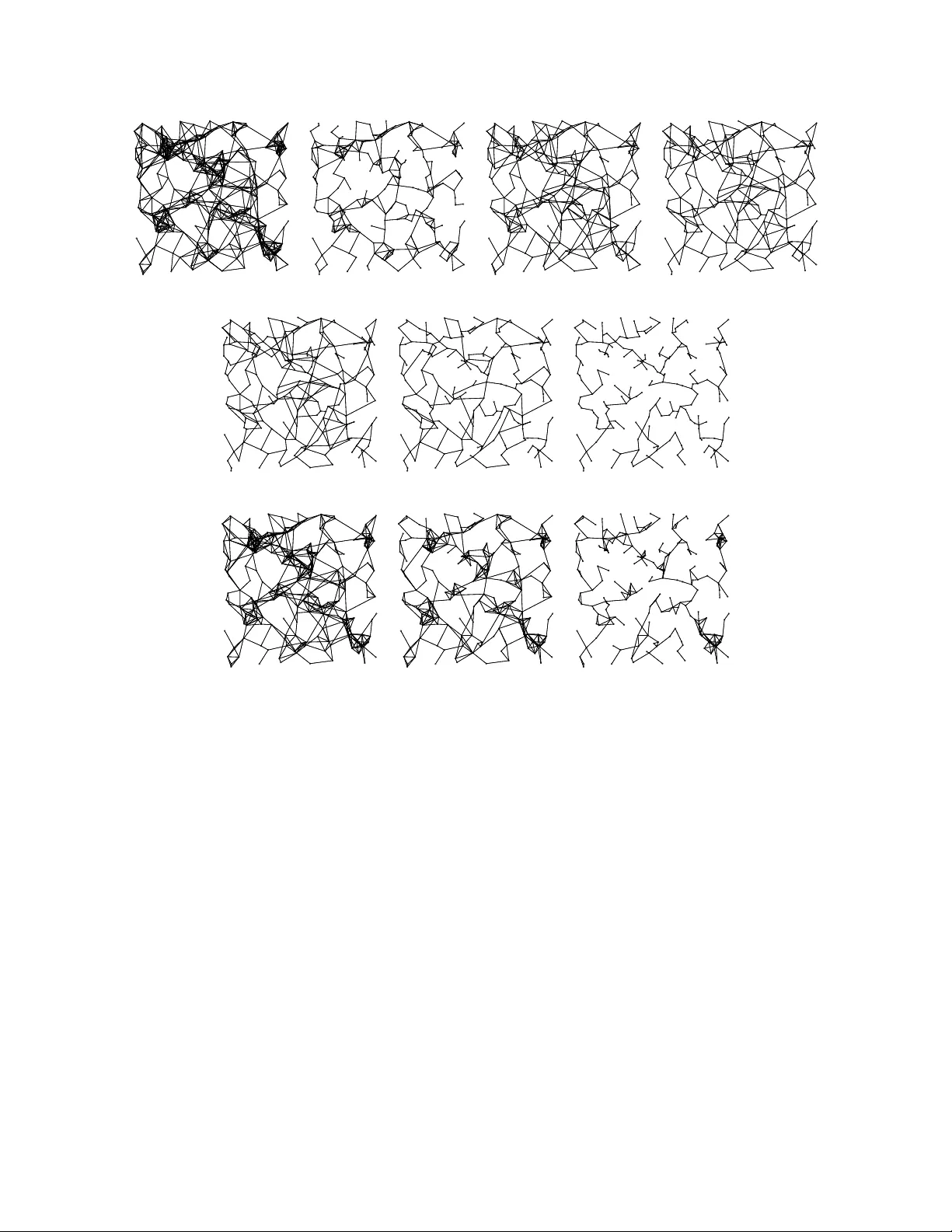
A Ne w Distrib uted T opology Control Algorithm for W ireless En vironments with Non-Uniform P ath Loss and Multipath Propagation Harish Sethu and Thomas Gerety Department of Electrical and Computer Engineering Drex el Univ ersity Philadelphia, P A 19104-2875 Email: { sethu, thomas.gerety } @drex el.edu Abstract Each node in a wireless multi-hop network can adjust the power lev el at which it transmits and thus change the topology of the network to sa ve ener gy by choosing the neighbors with which it directly communicates. Many pre vious algorithms for distributed topology control ha ve assumed an ability at each node to deduce some location-based information such as the direction and the distance of its neighbor nodes with respect to itself. Such a deduction of location-based information, howe ver , cannot be relied upon in real en vironments where the path loss exponents vary greatly leading to significant errors in distance estimates. Also, multipath effects may result in different signal paths with different loss characteristics, and none of these paths may be line-of-sight, making it difficult to estimate the direction of a neighboring node. In this paper, we present Step T opology Control (STC), a simple distributed topology control algorithm which reduces energy consumption while preserving the connectivity of a heterogeneous sensor network without use of any location-based information. The STC algorithm av oids the use of GPS de vices and also makes no assumptions about the distance and direction between neighboring nodes. W e show that the STC algorithm achiev es the same or better order of communication and computational complexity when compared to other known algorithms that also preserve connectivity without the use of location-based information. W e also present a detailed simulation-based comparati ve analysis of the energy sa vings and interference reduction achieved by the algorithms. The results sho w that, in spite of not incurring a higher communication or computational complexity , the STC algorithm performs better than other algorithms in uniform wireless en vironments and especially better when path loss characteristics are non-uniform. I . I N T RO D U C T I O N In a multi-hop wireless sensor network, a node communicates with another node across one or more consecuti ve wireless links with messages possibly passing through intermediate nodes. The topology of such a network can be vie wed as a graph with an edge connecting any pair of nodes that can communicate with each other directly without going through any intermediate nodes. Each node in such a network can choose its own neighbors and thus control the topology by changing the power at which it makes its transmissions or , in the case of nodes capable of directional transmissions, by also changing the set of directions in which it will allow transmissions. The goal of such topology control is to employ algorithms that each node can ex ecute in a distributed manner for the purposes of reducing energy consumption, maintaining connecti vity , and increasing network lifetime and/or capacity . In recent years, a lar ge number of topology control algorithms hav e been proposed and studied for a di verse set of goals [1]. Early work on topology control assumed that accurate location information about its neighbors will be av ailable to the nodes, such as through the use of GPS de vices [2]–[6]. This assumption adds to the expense of the nodes and also results in high delays due to the acquiring and tracking of satellite signals. Also, one cannot rely on GPS in man y real application en vironments such as inside buildings or thick forests. Some other topology control protocols that preserve connecti vity rely on the more likely ability of a node to estimate the distance and direction to its neighbors. For example, in the cone-based distributed topology control (CBTC) algorithms, a node u transmits with the minimum po wer p u,α required to ensure that there is some node it can reach within every cone of degree α around u [7]. Assuming a specific loss propagation model, the Euclidean distance to a neighbor can be deduced with kno wledge of the power at which a transmission is made by a neighbor and the power at which the signal is receiv ed. The direction of a neighbor with respect to itself can be deduced from the angle of arriv al of a signal. W ireless communication, howe ver , is often characterized by the phenomenon of multipath propagation wherein a signal reaches the receiving antenna via two or more paths [8]. In addition, there are several other kinds of radio irre gularities that ha ve an impact on the topology control algorithms [9]. The different paths, with differences in delay , attenuation, and phase shift, mak e it difficult for the recei ving node to deduce its distance from the sender and the direction of the sender . In this paper , we focus on the design of topology control algorithms that work without the use of any location-based information so that they can be employed in the presence of multipath propagation or when path loss exponents are non-uniform in the region of interest. More specifically , we focus on connecti vity-preserving algorithms that make no assumptions about the av ailability of GPS devices in nodes and no assumptions on the ability of a recei ving node to deduce either the distance or the direction of the sender . Besides accommodating the en vironmental causes of radio irregularities, we seek to also meet the requirements of a heterogeneous sensor network where (a) different nodes may have dif ferent maximum transmission po wers, and (b) v ariations in node/antenna configurations may lead to dif ferent reception thresholds in dif ferent directions. A. Pr oblem Statement Assume that each node u ∈ V is associated with a certain maximum po wer P u with which it is capable of making an omni-directional transmission (for ease of discussion, we use omni- 2 directional transmissions but our problem statement and the proposed algorithm can be readily adapted for directional transmissions). Note that we allow P u to be dif ferent for different nodes, allo wing a heterogeneous sensor network en vironment as in [10]. Consider the nodes in the network as vertices of a directed graph G m ax = ( V , E m ax ) in which nodes u and v are connected by a directed edge from u to v if and only if (a) an omni-directional transmission from u at its maximum power P u can directly reach v , and (b) an omni-directional transmission from v at its maximum power P v can directly reach u . Note that if ( u, v ) ∈ E m ax , then ( v , u ) ∈ E m ax . Many widely deployed MA C and address resolution protocols in wireless networks not only assume bidirectional links but also assume two-way handshakes and acknowledgments [11]. Therefore, with bidirectional communication assumed between directly communicating nodes, G m ax represents a realistic communication topology at maximum node powers. Gi ven G m ax = ( V , E m ax ) , the goal of topology control in this paper can be thought of as a multi-objecti ve optimization problem where we seek a ne w weighted directed graph G = ( V , E ) , E ⊆ E m ax . W e define P G ( u ) as the minimum power with which node u should make an omni- directional transmission so as to reach all of its neighbors in graph G . Let C G ( u ) denote the energy cost of a transmission by u at power P G ( u ) . 1 Assign weight C G ( u ) to each directed edge ( u, v ) ∈ E (all edges starting from a node ha ve the same weight since nodes in a sensor network broadcast messages at a certain constant power lev el determined by the topology control algorithm). Let C G ( s → t, E ner g y ) denote the sum of C G ( i ) for each transmitting node i in the minimum-energy path from node s to node t in the graph G (this represents the minimum energy cost for a message to trav erse from a source s to a destination t ). The multi-objectiv e problem is to find G with the following two objectiv es: 1) Minimize the av erage po wer , computed ov er all nodes, required in an omni-directional transmission by a node u to reach all of its neighbors in G . This objecti ve can be expressed as: min " X u ∈ V C G ( u ) # 2) Minimize the a verage energy cost, computed ov er all source-destination pairs, in a minimum- energy path from a source node to a destination node. This objectiv e can be expressed as: min   X s,t ∈ V C G ( s → t, E nerg y )   under the following constraints: 1) E ⊆ E m ax . 2) If ( u, v ) ∈ E , then ( v , u ) ∈ E , as is generally expected by MA C layer protocols. 3) If there exists a path between u and v in G m ax , then there also e xists a path between u and v in G (preserves connectivity). 1 Note that the power at which a node makes its transmissions is the energy consumed in the transmission per unit time. When the context is a single node, reducing po wer and reducing energy become the same goal because when we reduce transmission power at a giv en node, we also reduce energy consumption at the node. The energy consumption by the ov erall network, howe ver , is not al ways reduced when the transmission powers at the nodes are reduced. In this paper, we use the goals of reducing the energy cost and reducing the transmission po wer interchangeably when the context is limited to the transmissions by a single node. In the conte xt of an entire network, we speak of the goal of reducing energy costs. 3 01: Function STC at node ( u ) : 02: G ← ( V , φ ) /* directed graph with no edges */ 03: Compile outT upleList ( u ) and inT upleList ( u ) 04: Broadcast outT upleList ( u ) and inT upleList ( u ) at maximum power P u 05: Receiv e outT upleList ( n ) and inT upleList ( n ) from each neighbor n in G m ax 06: Compute fP airOfP aths ( n ) for each n two or fewer hops away from u 07: Compute bP airOfP aths ( n ) for each n two or fewer hops away from u 08: Sort outT upleList ( u ) 09: k ← degree of u in G m ax 10: do k − 1 times 11: t ( u, v ) ← the largest tuple in outT upleList ( u ) 12: remov e t ( u, v ) from outT upleList ( u ) 13: vSet = { i | t ( i, v ) ∈ i nT upl eList ( v ) , t ( i, v ) < t ( u, v ) } 14: NoF orwardP ath = T rue 15: NoBackwar dP ath = True 16: for n ∈ vSet 17: p = the first path in fP airOfP aths ( n ) without v 18: if max { r | r ∈ p } < t ( u, v ) 19: NoF orwardP ath = False 20: break (out of for loop) 21: end if 22: end for 23: vSet = { i | t ( v , i ) ∈ o utT upleList ( v ) , t ( v , i ) < t ( v , u ) } 24: for n ∈ vSet 25: p = the first path in bP airOfP aths ( n ) without v 26: if max { r | r ∈ p } < t ( v , u ) 27: NoBackwar dP ath = False 28: break (out of for loop) 29: end if 30: end for 31: if NoF orwar dP ath or NoBackwar dP ath 32: add a directed edge ( u, v ) to G 33: end if 34: end do Fig. 1. Pseudo-code description of the Step T opology Control algorithm at node u . The tw o objecti ves of minimizing the a verage transmission power of a node and minimizing the av erage energy cost along a minimum-energy path often work against each other . For example, minimizing av erage transmission power can lead to a very sparse graph with very long energy- expensi ve multi-hop paths between some pairs of nodes. B. Related W ork Let C ( u, v ) denote the minimum ener gy cost of a successful transmission from u to v . A topology control algorithm that minimizes energy consumption will remov e an edge ( u, v ) if 4 and only if there exists a path between u and v through an intermediate set of nodes n 1 , n 2 . . . n k such that C ( u, n 1 ) + C ( n 1 , n 2 ) + . . . C ( n k , v ) < C ( u, v ) . Accomplishing this requires a significant exchange of information between nodes and in such a case, the topology control algorithm is indistinguishable from a routing algorithm. As a result, a number of distrib uted topology control algorithms ha ve been proposed where nodes rely on lesser exchange of information between neighbors [1]. In this subsection, we focus on the subset of these protocols that can be adapted to work without the exchange of any location-based information between neighboring nodes. The KN EIGH protocol is based on determining the number of neighbors that each node should hav e in order to achie ve full connectivity with a high probability [12]. This protocol, ho wev er , does not guarantee connectivity e ven though it does achie ve connecti vity with a high probability . The Small Minimum-Energy Communication Network (SMECN) protocol [4] seeks to achiev e a lo wer energy cost while guaranteeing connectivity by removing an edge ( u, v ) if and only if there exists a path u → n → v such that C ( u, n ) + C ( n, v ) < C ( u, v ) . As proposed in [4], the protocol requires the use of GPS devices b ut the same results can be accomplished if each node exchanges information with each of its neighbors re garding the energy costs of reaching all of its neighbors. When used with some of the widely av ailable routing algorithm implementations such as A OD V or DSR that base their decisions on the number of hops in a path rather than the total energy cost of the path, the SMECN protocol does not necessarily result in a significant reduction in energy consumption. As will be shown in Section IV, the energy savings achiev ed by SMECN is not significantly greater e ven if the routing algorithm were to choose a minimum-energy path. The Directed Relati ve Neighborhood Graph (DRNG) protocol [10] removes an edge ( u, v ) if and only if there exists a path u → n → v such that max { C ( u, n ) , C ( n, v ) } < C ( u, v ) . In the Directed Local Spanning Subgraph (DLSS) protocol [10], each node creates a local spanning tree from the subgraph induced by itself and its neighbors. A node u retains the edge ( u, v ) in the topology-controlled graph if and only if the edge ( u, v ) exists in the local spanning tree generated at node u . As prov ed in [10], any edge that is remov ed by DRNG is also remov ed by DLSS and therefore, DLSS achie ves a sparser graph than DRNG. The fewer edges in DLSS often leads to a lower energy consumption, but it can sometimes lead to longer paths and therefore higher energy consumption than DRNG. A generalization of the DRNG protocol is the XTC protocol which was conceiv ed independently and uses the notion of ‘link quality’ in making its topology control decision instead of energy costs [13]. When link quality between two nodes is measured by the energy cost of a transmission between them, the XTC protocol reduces to DRNG. Among other attempts to accommodate the irregularities of a real wireless en vironment in topology control are some that allo w for uncertainties in whether or not a nearby node is reachable if the distance to that node is above a certain threshold [14], [15]. Howe ver , these algorithms assume that each node can know the distances to other nearby nodes, something that cannot be relied upon in a real en vironments with multipath ef fects. Some other works ha ve also considered realistic wireless models but they hav e only presented centralized algorithms [16]. C. Contributions In this paper , we present the Step T opology Control (STC) algorithm in which a node u remov es an edge ( u, v ) if and only if there exists: 5 • a path with three or fewer hops from u to v such that the energy cost across each hop is less than C ( u, v ) . • a path with three or fewer hops from v to u such that the ener gy cost across each hop is less than C ( v , u ) . The STC algorithm relies on each node exchanging information with each of its neighbors regarding the energy costs of communication to all of its neighbors. The STC algorithm may be seen as an extension of the DRNG algorithm to allow a search for three-hop paths and to ensure bidirectional communication between directly communicating nodes. Ho wev er , our implementation of the algorithm ensures that the order of communication and the computational comple xity do not increase despite a search for three-hop paths. This search for three-hop paths makes only a small impact on performance when the wireless en vi- ronment is uniform across the netw ork. Ho wev er , it makes a significant impact when a more realistic scenario is assumed with multipath propagation and other irregularities in the path loss characteristics in the wireless en vironment. In such en vironments, the STC algorithm achie ves a much lo wer energy consumption and interference than other topology control algorithms in spite of maintaining the same or better order of communication and computational complexity . W e also show that this improv ed performance of the STC algorithm exists largely independent of the size of the network. Section II presents the STC algorithm along with a pseudo-code description. Section III presents an analysis of the communication and computational complexity of the STC algorithm and presents a comparativ e analysis. Section IV presents se veral simulation-based results that provide a thorough comparison of the energy consumption properties of the STC algorithm and other existing topology control strategies that can be adapted to use no location-based information. In particular , we examine the algorithms in environments with both constant and v aried path loss exponents and study their scalability in performance as the number of nodes increases. Section V concludes the paper with a summary of its findings and future research directions. A proof of the relationship between the STC algorithm and a CBTC algorithm with all applicable optimizations is presented in the Appendix. I I . S T E P T O P O L O G Y C O N T R O L Denote by P m in ( u, v ) , the minimum power necessary for a transmission from u to reach v , otherwise kno wn as transmission power thr eshold . W e allo w that P m in ( u, v ) is not necessarily the same as P m in ( v , u ) . The basic idea behind the Step T opology Control (STC) algorithm is to find both forward and backward paths with three or fewer hops between u and v such that each hop requires a lower ener gy cost than that required for an equiv alent direct transmission between u and v . If such multi-hop paths exist between u and v , node u drops the edge ( u, v ) from the directed graph it generates and node v similarly drops the edge ( v , u ) . The STC algorithm relies on being able to uniquely order the energy costs of transmissions across nodes. Since the power lev els at which transmissions are made may take on only certain discrete values in some systems, we add additional identifiers to permit a unique ordering. W e assume that each node u is uniquely identified by an integer ID u . For each ordered pair of nodes u and v , we associate an ordered tuple t ( u, v ) = ( t 1 , t 2 , t 3 ) , where t 1 = P m in ( u, v ) , t 2 = ID u , and t 3 = ID v . W e say that ( t 1 , t 2 , t 3 ) < ( t 0 1 , t 0 2 , t 0 3 ) if and only if (1) t 1 < t 0 1 , or (2) t 1 = t 0 1 and t 2 < t 0 2 , or (3) t 1 = t 0 1 , t 2 = t 0 2 , and t 3 < t 0 3 . For the sake of completeness, we define 6 t ( u, u ) < t ( x, y ) for any u and x 6 = y since a transmission to itself should cost less energy than a transmission to another node. Note that t ( u, v ) and t ( v , u ) are strictly ordered by the above lexicographic rule and not equal ev en if the minimum power required for transmission between u and v is the same in either direction. W e call t ( u, v ) a transmission tuple. A path p in the graph consists of an ordered sequence of transmission tuples. Denote by maxT uple ( p ) the largest tuple in path p . Consider any two nodes u and v such that ( u, v ) ∈ E m ax . W e assume that u can determine the minimum power necessary for its transmission to reach v as well as the minimum power required for a transmission from v to reach itself. This is accomplished by transmitting beacon messages at increasing powers and noting the power at which each neighbor is first discovered. Each beacon message carries within it the power at which it is transmitted so that the disco vered neighbor may also note the minimum power necessary for it to be reached by a neighboring node. Each node u can thus compile two lists of transmission tuples: outT upleList ( u ) containing t ( u, v ) for all ( u, v ) ∈ E m ax , and inT upleList ( u ) containing t ( v , u ) for all ( v , u ) ∈ E m ax . This process of exchanging po wer le vel information is feasible in practice and is part of many proposed energy-a ware MA C layer protocols as well as topology control algorithms such as DLSS. Figure 1 presents a pseudo-code description of the STC algorithm. Once a node u compiles outT upleList ( u ) and inT upleList ( u ) , it begins ex ecution of the algorithm. Each node u first broadcasts both its inT upleList and outT upleList at its maximum power P u to reach all of its neighbors (line 04). The node also collects the inT upleLists and outT upleLists from each of its neighbors (line 05). Gi ven all this information about the ener gy costs, node u computes two forward paths (denoted fP airOfP aths ( n ) ) and two backward paths (denoted bP airOfP aths ( n ) ) for each node n that is reachable by two or fewer hops (lines 06–07). W e describe below in greater detail the construction of the forward path data structures for node n (the construction of the backward pair of paths is similar). Let p 1 denote the first of the pair of paths in fP airOfP aths ( n ) and let p 2 denote the second. W e choose p 1 and p 2 such that maxT uple ( p 1 ) < maxT uple ( p 2 ) < maxT uple ( p ) where p is any path of two or fewer hops from u to n other than p 1 and p 2 . In lines 16–22, this data structure allows the node to quickly determine if there exists a path s of three or fewer hops between u and another node v such that maxT uple ( s ) < t ( u, v ) . The reason we need a pair of paths instead of just one path is because one of these paths may be through v and one would not choose to replace the edge ( u, v ) with a path that goes through v . Node u then orders the tuples in its outT upleList ( u ) (line 08) and considers each of the edges ( u, v ) in rev erse lexicographical order of the associated tuples t ( u, v ) , i.e., the neighbor that requires the lar gest po wer to be reached is considered first (line 11). As each neighbor v is processed, the corresponding tuple t ( u, v ) is remov ed from outT upleList ( u ) (line 12). T o determine if an edge ( u, v ) should be removed, a node u looks for a forward path u → n 1 → n 2 → v , where the nodes n 1 and n 2 may or may not be distinct (lines 13– 22). The condition that the path should satisfy is max { t ( u, n 1 ) , t ( n 1 , n 2 ) , t ( n 2 , v ) } < t ( u, v ) . The node similarly seeks to find a re verse path via nodes n 3 and n 4 (lines 23–33) such that max { t ( v , n 3 ) , t ( n 3 , n 4 ) , t ( n 4 , u ) } < t ( v , u ) . Note that the number of distinct nodes among n 1 , n 2 , n 3 and n 4 may range anywhere between 1 and 4. If both forw ard and backw ard two- or three-hop paths are found satisfying the desired conditions on the tuples, the edge ( u, v ) is remov ed from the graph (lines 31–33). 7 T o determine if there e xists a forward path from u to v satisfying the desired conditions, node u first constructs the set vSet consisting of nodes i that are neighbors of v such that t ( i, v ) < t ( u, v ) (line 13). Now , if there exists a path, p , of two or fewer hops from u to any node in vSet such that the path is not through v and maxT uple ( p ) < t ( u, v ) , then the condition for the forward path is satisfied. This is determined in lines 16–22 and the existence of a backward path is similarly determined in lines 24–30. I I I . C O M P A R A T I V E A NA LY S I S In this section, we discuss the communication and computational complexity of the STC algorithm in comparison to other topology control algorithms that also preserve connectivity while being capable of operation in real en vironments with multipath propagation or non- uniform path loss exponents. W e also discuss any prov able relationships between STC and other algorithms regarding the set of edges remov ed from G m ax by the algorithm. A. Complexity W e consider the complexity of the following algorithms and present a comparison to the STC algorithm: • Small Minimum Energy Communication Network (SMECN). • Directed Relati ve Neighborhood Graph (DRNG). • Directed Local Spanning Subgraph (DLSS). Each of the above algorithms relies on each node first determining the energy cost to each of its neighbors. As explained in Section II, this can be accomplished by transmitting beacon messages at increasing powers and noting the power at which each neighbor is first discovered. When beacon messages carry the po wer at which they are being transmitted, each node can also learn the energy cost of the communication from each of its neighbors to itself. Depending on the granularity of po wer le vels at which transmissions can be made, a variety of strategies based on linear or binary search methods may be employed in these steps to minimize interference and to maximize speed of con ver gence to the correct po wer values. W e do not include this step in our complexity analysis because it is common to all topology control protocols abov e and cannot be considered a distinguishing feature of STC or any other specific protocol. T opology control algorithms begin with the assumption that each node can determine and will know the minimum po wer at which it should transmit to reach another particular node. For the STC algorithm, for example, we consider its complexity at node u after the compilation of outT upleList ( u ) and inT upleList ( u ) is complete. In the original graph, G m ax , on which a topology control algorithm is ex ecuted, the in-degree of a node is the same as its out-degree (since bidirectional communication is assumed) and therefore, the maximum out-degree ( ∆ + ) and the maximum in-degree ( ∆ − ) are identical. W e define the node-degree of a node in G m ax as the number of its neighbors that it communicates with, i.e., its out-degree or its in-degree. In the following, we denote the maximum node-degree of the original graph by ∆ = ∆ + = ∆ − . Further , in our analysis, we do not include the ID size in computing the communication complexity . This is because the IDs on sensor nodes are likely to be globally unique for each node and assigned by the manufacturer , as in the case of Ethernet cards. W e expect the ID sizes, therefore, to be independent of the size of the sensor network deployment. 8 Algorithm Communication Comple xity Computational Comple xity SMECN O (∆ 2 ) O (∆ 2 ) DRNG O (∆ 2 ) O (∆ 2 ) DLSS O (∆ 2 ) O (∆ 2 log ∆) STC O (∆ 2 ) O (∆ 2 ) T ABLE I A C O M PAR I S O N B E T W E E N T O P O L O G Y C O N T R O L A L G O R I T H M S Theor em 3.1: The communication complexity of the STC algorithm is O (∆ 2 ) . Pr oof: For any giv en node n , the lists inT upleList ( n ) and outT upleList ( n ) are each of length O (∆) . Broadcasting the lists (line 04 in Figure 1), therefore, is O (∆) in communication complexity and receiving the lists from each of up to ∆ neighbors (line 05) is O (∆ 2 ) in communication complexity . The ov erall communication complexity , therefore, is O (∆ 2 ) . Theor em 3.2: The computational complexity of the STC algorithm is O (∆ 2 ) . Pr oof: For each neighbor n 0 of u , one can process the entries in the outT upleList ( n 0 ) to create the pair of paths in fP airOfP aths . The determination of whether or not a path to node n should be included in fP airOfP aths and whether it should be the first or the second of the pair of paths can be made in O (1) time since it in volv es no more than two tuple comparisons. Let h denote the number of one-hop or two-hop paths starting from u . Since h = O (∆ 2 ) , creating the fP airOfP aths will require a total time of O (∆ 2 ) . Creating the bP airOfP aths will similarly require a total time of O (∆ 2 ) . Sorting of the outT upleList ( u ) in line 08 takes time O (∆ log ∆) since the size of the list is O (∆) . W e no w sho w that the 2 h pairs of paths created abov e can allo w the inner for loops of lines 16–22 and 24–30 to complete in time O (∆) . It is readily verified that each iteration of the for loops completes in O (1) time (lines 17–21 and 25–29). Since the size of the vSet is O (∆) , these inner for loops e xecute in O (∆) time. The only other non-loop component inside the outer do loop between lines 10–34 that takes more than O (1) time is the creation of the vSet itself, which takes O (∆) time. Since the do loop iterates k − 1 times where k ≤ ∆ , the entire do loop completes in time O (∆ 2 ) . The overall computational complexity of the STC algorithm, therefore, is O (∆ 2 ) . T able I presents a comparison of the communication and computational complexities of topology control algorithms that preserve connectivity and which do not employ the exchange of any location-based information between neighbors. All in volv e a communication complexity of O (∆ 2 ) since they all require that each node collect a list of energy costs from each of its neighbors. In the computational complexity analysis of DLSS, we consider the number of nodes in the local graph as O (∆) and the number of edges as O (∆ 2 ) . The computation of the local minimum spanning tree, assuming Kruskal’ s algorithm [17], is O (∆ 2 log ∆) . 9 B. Set of edges r emoved The SMECN, DRNG and DLSS algorithms allo w directed edges in the graph they generate. Since STC assumes bidirectional links motiv ated by the need of real MA C layer protocols, in order to make a fair comparison, we will assume that energy costs are the same in both forward and rev erse directions (so that SMECN, DRNG and DLSS will also lead to only undirected edges in the graphs they generate). Under this assumption, the STC algorithm remov es any edge from the original graph that is also remov ed by SMECN or DRNG. The SMECN algorithm remov es an edge ( u, v ) if there exists a two-hop path from u to v through n such that C ( u, n ) + C ( n, v ) < C ( u, v ) . Therefore, we hav e C ( u, n ) < C ( u, v ) and C ( n, v ) < C ( u, v ) which would be the condition that will lead the DRNG or STC algorithm to also remove edge ( u, v ) . Assuming that the ener gy costs are the same in both forward and rev erse directions, the STC algorithm becomes a simple extension of the DRNG algorithm, and therefore, it is easily argued that it will remove all edges that are remov ed by DRNG. Thus, the STC algorithm yields a lo wer energy cost per transmission at any giv en node than either SMECN or DRNG under these conditions. Howe ver , the STC algorithm does not al ways remove an edge that would be removed by DLSS. F or a comparati ve analysis with the DLSS algorithm, we rely on the simulation results presented in the next section. It is of interest to note that the STC algorithm is related to the OPT -CBTC( 5 π / 6 ) algorithm (which is the CBTC( 5 π / 6 ) algorithm with all applicable optimizations). The STC algorithm remov es all edges that would be remo ved by OPT -CBTC( 5 π / 6 ). As a result of this relationship, prov ed in Appendix A, the STC algorithm exhibits some of the same angular properties as OPT -CBTC( 5 π / 6 ). Since DRNG, DLSS and STC do not necessarily reduce energy costs in the path from u to v each time they remove an edge ( u, v ) , rare pathological cases are possible where these algorithms significantly increase energy costs. Consider an edge ( u, v ) corresponding to an ener gy cost of C ( u, v ) . It is possible that the STC algorithm remov es this edge because there exist three other edges, each corresponding to an energy cost of C ( u, v ) −  , where  is an infinitesimal quantity (thus almost tripling the energy cost between u and v ). These three edges, in turn may be remov ed because each can be replaced by three edges corresponding to ener gy costs of C ( u, v ) − 2  , which no w multiplies the total ener gy cost between u and v by nine. Such scenarios are rare in real situations and our simulation results, described in the next section, show that when nodes are scattered randomly in a region, the STC algorithm actually performs significantly better than the other algorithms considered in this paper . I V . S I M U L A T I O N R E S U L T S In this section, we present a simulation-based comparativ e study of the following distributed topology control algorithms: • Step T opology Control (STC), the algorithm presented in this paper . • OPT -CBTC( 5 π / 6 ), as a representativ e CBTC algorithm and because of its relationship to the STC algorithm. • Small Minimum Energy Communication Network (SMECN). • Directed Relati ve Neighborhood Graph (DRNG). • Directed Local Spanning Subgraph (DLSS). 10 The XTC protocol uses the notion of ‘link quality’ in generating the output topology [13]. When the link quality is measured by the energy cost of a transmission across the link, the XTC protocol reduces to the DRNG protocol. Therefore, the XTC protocol is not separately included in these comparisons. In addition to the above, we use the follo wing two additional algorithmic metrics as references on the performance bounds of topology control algorithms: • Minimum Spanning T r ee (MST): The MST achie ves the first stated objecti ve of the topology control problem described in Section I-A. The MST preserves connectivity while minimizing the average power (computed ov er all nodes) with which a node makes its transmissions. • MinReac h: In MinReach, each transmission from a node to one of its neighbors uses exactly the minimum energy required to reach that particular neighbor (as opposed to each node making all its transmissions to any neighbor at the same po wer le vel). The total energy cost of transmissions from a source to a destination along the minimum energy path using MinReach is a lo wer bound (though, not a tight lo wer bound) on the total energy cost along a path between the source-destination pair 2 . A. Metrics Assume P u = P for all nodes u (recall that P u denotes the maximum po wer with which a node u can transmit). If the power P is assumed to be an arbitrary quantity in our simulations, the reduction in energy achie ved by topology control algorithms can be misleading (if P is arbitrarily large, the reduction will be similarly large). Therefore, in our simulations, we assume the smallest possible value of P so that the original graph used as the input to the topology algorithm is connected. This offers a standardized approach to estimating the ef fectiv eness of topology control algorithms so that arbitrarily large reductions in energy consumption cannot be claimed by topology control algorithms by simply using a dense highly-connected G m ax . For each network, the baseline for our comparisons is the initial graph, H , defined as follows. Consider graph G generated by creating an edge ( u, v ) from u to v if and only if a transmission from u at power p can reach v and a transmission from v to u at po wer p can reach u . Note that, when p = P , G = G m ax . Let P H denote the minimum v alue of p at which G is connected. The graph G generated by each node transmitting at power P H is the initial graph, H . Gi ven a graph, T 0 , generated by the ex ecution of the topology control algorithm, we define P T 0 ( u ) as the minimum po wer with which node u should make an omni-directional transmission so as to reach all of its neighbors in graph T 0 . Let C T 0 ( u ) denote the ener gy cost of a transmission by u at power P T 0 ( u ) . Gi ven the graph T 0 abov e, we define a new graph T as follo ws: a node u is connected by an edge to v in T if and only if C T 0 ( u ) > C ( u, v ) or C T 0 ( v ) > C ( v , u ) . Thus, giv en omni-directional transmissions, T represents the graph that is actually relev ant for performance comparisons and, especially , interference comparisons. T , as opposed to T 0 , also enforces the ability for bidirectional transmissions between communicating nodes. W e call T the cover graph generated by the topology control algorithm. All of our simulation results use the cover graph. 2 Some other topology control algorithms, such as a distrib uted algorithm for constructing a Gabriel Graph [18], cannot serve as optimal solutions or lower bounds in our case where different nodes may ha ve dif ferent maximum transmission powers and where path loss e xponents may vary in different directions for the same transmitting node. 11 Define P T ( u ) as the minimum power with which node u should make an omni-directional transmission so as to reach all of its neighbors in the co ver graph T . Let C T ( u ) denote the ener gy cost of a transmission by u at power P T ( u ) . Note that P T ( u ) ≥ P T 0 ( u ) and C T ( u ) ≥ C T 0 ( u ) . In our simulations, we use P T ( u ) as the po wer at which node u makes all its transmissions after the execution of a topology control algorithm generating cover graph T . P T ( u ) /P H , denoted by P T /H ( u ) , is the ratio of the power at which node u transmits after the ex ecution of the topology control algorithm that generates cov er graph T and the power at which it transmits in the initial graph, H . W ith this normalization to the energy costs in the initial graph, this ratio captures the energy savings per transmission due to the topology control algorithm. Let C T ( u → v , H ops ) denote the sum of C T ( i ) for each transmitting node i in the minimum- hop path from u to v in cov er graph T . C T ( u → v , H ops ) /C H ( u → v , H ops ) , denoted by C T /H ( u → v , H ops ) , is the ratio of the energy cost along the minimum-hop path from u to v in cov er graph T generated by the topology control algorithm and the corresponding cost along the minimum-hop path from u to v in the initial graph, H . This ratio captures the ener gy sa vings along a path due to the topology control algorithm. In our simulation experiments, we examine both the minimum-energy paths and the minimum-hop paths. The ratio for the minimum-energy paths is computed similarly as above and is denoted by C T /H ( u → v , E ner g y ) . Our measure of interference deriv es from the definition in [20], which is a refinement of that used in [21]. Define the span, span ( e ) , of an edge e = ( g , h ) as the number of nodes that are neighbors of at least one of g and h . This represents the number of nodes that would have to remain silent to enable a successful transmission between g and h . W e measure interference, I T ( u → v , H ops ) , along the minimum-hop path from u to v in cover graph T as the sum of span ( e ) for all e in the path. I T /H ( u → v , H ops ) denotes the ratio of the interference along the minimum-hop path from u to v in cover graph T generated by the topology control algorithm and the corresponding cost along the minimum-hop path from u to v in the initial graph, H . This ratio represents the reduction in interference achiev ed due to the topology control algorithm. The ratio for the minimum-energy paths is computed similarly as abov e and is denoted by I T /H ( u → v , E ner g y ) . B. W ir eless Model The pertinent issue in the modeling of the wireless en vironment in the context of this paper is the path loss model. The log-distance path loss model based on the path loss as a logarithmic function of the distance d has been confirmed both theoretically and by measurements in a large v ariety of en vironments [19]. In this model, the path loss at distance d , P L ( d ) is expressed as: P L ( d ) = P L ( d 0 ) + 10 γ log 10 ( d/d 0 ) where the constant d 0 is an arbitrary reference distance and γ is called the path loss exponent. The path loss e xponent is an important parameter in modeling a wireless en vironment and v aries within a re gion depending upon a number of f actors including antenna characteristics, transmission frequency , the nature of the obstructions, multipath, and shado wing effects. While most of these effects are location-specific and dif ficult to generalize across different en vironments [22], empirical observ ations in se veral real en vironments do re veal that the distribution of path loss exponents within a region of interest is Gaussian [23]–[26]. Our simulation models, 12 0 0 . 1 0 . 2 0 . 3 0 . 4 0 . 5 0 . 6 0 . 7 0 . 8 0 . 9 1 Avg. energy cost per transmission Avg. energy cost per transmission 1 . 5 2 2 . 5 3 3 . 5 Path Loss Exp onent Path Loss Exp onent None OPT-CBTC(5 π/ 6) SMECN DRNG DLSS STC MST (lower bound) (a) A verage P T /H ( u ) o ver all u . 0 0 . 1 0 . 2 0 . 3 0 . 4 0 . 5 0 . 6 0 . 7 0 . 8 0 . 9 1 1 . 1 1 . 2 1 . 3 Avg. energy cost along min-energy path Avg. energy cost along min-energy path 1 . 5 2 2 . 5 3 3 . 5 Path Loss Exp onent Path Loss Exponent None OPT-CBTC(5 π/ 6) SMECN DRNG DLSS STC MST MinReach (low er bound) (b) C T /H ( u → v , E ner g y ) av eraged o ver all pairs of nodes u and v . 0 1 2 3 4 5 6 7 8 9 Average node-degree Average node-degree 1 . 5 2 2 . 5 3 3 . 5 Path Loss Exponent Path Loss Exponent None OPT-CBTC(5 π/ 6) SMECN DRNG DLSS STC MST (c) A verage node-de gree. 0 . 4 0 . 5 0 . 6 0 . 7 0 . 8 0 . 9 1 1 . 1 1 . 2 1 . 3 Avg. energy cost along min-hop path Avg. energy cost along min-hop path 1 . 5 2 2 . 5 3 3 . 5 Path Loss Exp onent Path Loss Exponent None OPT-CBTC(5 π/ 6) SMECN DRNG DLSS STC MST (d) C T /H ( u → v , H ops ) a veraged o ver all pairs of nodes u and v . 0 . 6 0 . 65 0 . 7 0 . 75 0 . 8 0 . 85 0 . 9 0 . 95 1 1 . 05 1 . 1 1 . 15 1 . 2 1 . 25 1 . 3 Avg. in terference along min-hop path Avg. in terference along min-hop path 1 . 5 2 2 . 5 3 3 . 5 Path Loss Exp onent Path Loss Exp onent None OPT-CBTC(5 π/ 6) SMECN DRNG DLSS STC MST (e) I T /H ( u → v , H ops ) averaged over all pairs of nodes u and v . 0 . 6 0 . 65 0 . 7 0 . 75 0 . 8 0 . 85 0 . 9 0 . 95 1 1 . 05 1 . 1 1 . 15 1 . 2 1 . 25 1 . 3 Avg. in terference along min-energy path Avg. in terference along min-energy path 1 . 5 2 2 . 5 3 3 . 5 Path Loss Exp onent Path Loss Exp onent None OPT-CBTC(5 π/ 6) SMECN DRNG DLSS STC MST (f) I T /H ( u → v , E nerg y ) averaged over all pairs of nodes u and v . Fig. 2. Graphs sho wing the effecti veness of topology control algorithms when the path loss exponent is the same across the entire re gion of the network (in order to allo w comparisons with the CBTC algorithms). The networks are generated with 200 randomly located nodes in a unit square area. Each data point represents an average of one hundred random networks. Note that a longer distance between two nodes does not necessarily mean higher energy cost across the pair since path loss exponents follow a random Gaussian distribution. 13 0 0 . 1 0 . 2 0 . 3 0 . 4 0 . 5 0 . 6 0 . 7 0 . 8 0 . 9 1 Avg. energy cost per transmission 0 0 . 05 0 . 1 0 . 15 0 . 2 0 . 25 0 . 3 0 . 35 0 . 4 Standard Deviation of Path Loss Exponent V alues ( σ ) None SMECN DRNG DLSS STC MST (lower bound) (a) A verage P T /H ( u ) o ver all u . 0 . 2 0 . 3 0 . 4 0 . 5 0 . 6 0 . 7 0 . 8 0 . 9 1 Avg. energy cost along min-energy path 0 0 . 05 0 . 1 0 . 15 0 . 2 0 . 25 0 . 3 0 . 35 0 . 4 Standard Deviation of Path Loss Exponent V alues ( σ ) None SMECN DRNG DLSS STC MinReach (low er bound) (b) C T /H ( u → v , E ner g y ) av eraged o ver all pairs of nodes u and v . 1 2 3 4 5 6 7 8 9 Average node-degree 0 0 . 05 0 . 1 0 . 15 0 . 2 0 . 25 0 . 3 0 . 35 0 . 4 Standard Deviation of P ath Loss Exp onent V alues ( σ ) None SMECN DRNG DLSS STC (c) A verage node-de gree. 0 . 5 0 . 6 0 . 7 0 . 8 0 . 9 1 Avg. energy cost along min-hop path 0 0 . 05 0 . 1 0 . 15 0 . 2 0 . 25 0 . 3 0 . 35 0 . 4 Standard Deviation of Path Loss Exponent V alues ( σ ) None SMECN DRNG DLSS STC (d) C T /H ( u → v , H ops ) a veraged o ver all pairs of nodes u and v . 0 . 8 0 . 85 0 . 9 0 . 95 1 Avg. in terference along min-hop path 0 0 . 05 0 . 1 0 . 15 0 . 2 0 . 25 0 . 3 0 . 35 0 . 4 Standard Deviation of Path Loss Exponent V alues ( σ ) None SMECN DRNG DLSS STC (e) I T /H ( u → v , H ops ) averaged over all pairs of nodes u and v . 0 . 8 0 . 85 0 . 9 0 . 95 1 Avg. in terference along min-energy path 0 0 . 05 0 . 1 0 . 15 0 . 2 0 . 25 0 . 3 0 . 35 0 . 4 Standard Deviation of Path Loss Exponent V alues ( σ ) None SMECN DRNG DLSS STC (f) I T /H ( u → v , E nerg y ) averaged over all pairs of nodes u and v . Fig. 3. Graphs showing the effecti veness of topology control algorithms in reducing energy costs when the path loss exponents exhibit a Gaussian distribution with a mean of 3.1 in the range [2 . 7 , 3 . 5] for various values of the standard deviation (indoor propagation [19]). The networks are generated with 200 randomly located nodes in a unit square area. accordingly , use a Gaussian distribution when the path loss exponent is assumed to v ary across the region of interest. 14 0 0 . 1 0 . 2 0 . 3 0 . 4 0 . 5 0 . 6 0 . 7 0 . 8 0 . 9 1 Avg. energy cost per transmission Avg. energy cost per transmission 100 150 200 250 300 350 400 450 500 Number of sensor no des Number of sensor no des None SMECN DRNG DLSS STC MST (lower bound) (a) A verage P T /H ( u ) over all u . 0 0 . 1 0 . 2 0 . 3 0 . 4 0 . 5 0 . 6 0 . 7 0 . 8 0 . 9 1 Avg. energy cost along min-energy path Avg. energy cost along min-energy path 100 150 200 250 300 350 400 450 500 Number of sensor no des Number of sensor no des None SMECN DRNG DLSS STC MinReach (low er b ound) (b) C T /H ( u → v , E ner g y ) averaged ov er all pairs of nodes u and v . Fig. 4. Graphs showing the effecti veness of topology control algorithms in reducing energy costs when the path loss exponent varies around a mean of 3.1 with a standard deviation of 0.16 (indoor propagation [19]). The graphs show that the effecti veness of the STC algorithm (for that matter, all localized topology control algorithms) do not change with increase in the number of nodes. In our simulation studies, the specific values of the path loss exponents and the standard de viation of their distribution are based on results from empirical studies of indoor propagation described in [19]. W e choose the indoor propagation model because the constraints on topology control specifically considered in this paper , such as having to a void a GPS recei ver and not being able to discern the direction of signal arri val, are most applicable to indoor wireless en vironments. Our study uses three sets of simulation experiments in comparing the effecti veness of dif ferent topology control algorithms. In the first set of experiments, we assume that the path loss exponent is the same across the entire network and study the topology control algorithms for dif ferent v alues of the path loss exponent between 1.5 to 3.5. These experiments are intended to rev eal the dependence of topology control performance on the path loss exponent and to allow a comparison to CBTC algorithms (since they assume a uniform path loss exponent across the entire region). This first set of experiments is not intended to simulate a real wireless en vironment. In the second set of experiments, we vary the path loss exponent randomly using a truncated Gaussian distribution, as suggested in [23] for simulation experiments. Based on empirical measurements of indoor propagation at 634 locations in buildings [19], the path loss exponents in our experiment follow a truncated Gaussian distribution between 2.7 and 3.5 with a mean of 3.1. W e v ary the standard deviation of the distribution from 0 to 0.4 to study the impact of the spatial variation of path loss exponents on the performance of topology control algorithms. In the third set of experiments, we study the effecti veness of the algorithms as the number of nodes increases. The networks used in our first two sets of experiments consist of 200 nodes located randomly in a unit square area. In the third set of experiments, we vary the number of nodes from 100 to 500 to study the scalability of the algorithms across a fi ve-fold increase in the number of nodes. In these experiments also, we use a truncated Gaussian distribution for the path loss exponents ranging from 2.7 to 3.5 with a mean of 3.1. Howe ver , we use a single standard deviation of 0.16 (based on scatter plots from the empirical measurements of indoor 15 propagation on a single floor of a b uilding, described in [19]). Each data point in this paper represents an av erage of one hundred dif ferent randomly generated networks. Finally , we note that DRNG and STC algorithms can be generalized by a parameter k so that an edge ( u, v ) is removed when there exists a path of k hops or less from u to v and from v to u provided the energy cost across each of these hops is less than that corresponding to a direct transmission between u and v . In the fourth set of experiments, we examine the dependence of our key performance metrics on k . Our simulation model, because it is based on empirical measurements in real wireless en- vironments, encapsulates multipath and other phenomena such as shadowing common in real en vironments. The follo wing describes each of the simulation experiments and the results in greater detail. C. Experiment 1 W e include the CBTC algorithms in our first set of simulation experiments. The CBTC algorithms, howe ver , assume that the loss propagation characteristics of the medium are uniform across the entire re gion. In fairness to the CBTC algorithms, therefore, we conduct this simulation experiment with identical path loss exponents between any pair of directly communicating nodes in the network. For path loss exponents ranging from 1.5 to 3.5, we first pro vide results on the two objecti ves of the topology control problem statement described in I-A. Figure 2(a) presents the ratio P T /H ( u ) av eraged ov er all nodes. The cov er graph of the minimum spanning tree (MST) represents the lo wer bound of the achiev able average P T /H ( u ) and is also plotted in the graph. Figure 2(b) plots the ratio C T /H ( u → v , E ner g y ) av eraged over all pairs of nodes u and v . The result obtained for MinReach represents the lower bound on the average energy costs along a path. Note that the MST graph which achieves the lower bound for the first objecti ve does very poorly on the second objecti ve of minimizing the energy cost along paths. This is because the MST graph has far too fe w edges leading to unnecessarily long multi-hop paths. In fact, the MST graph is worse than no topology control at all for low v alues of path loss exponents. Figure 2(c) plots the av erage node-degree of a node in the cover graphs generated by the topology control algorithms. SMECN is the only algorithm for which the a verage node de gree v aries substantially with a change in the path loss exponent. This is because SMECN makes a comparison between the energy cost along an edge with the sum of the energy costs along other edges. The result of such a comparison changes with the assumed value of the path loss exponent and therefore, SMECN results in different topologies under different values of the path loss e xponent. All other algorithms are based on one-to-one comparison of edges as reg ards their energy costs, and the result of such comparisons is the same independent of the path loss exponent as long as the same path loss exponent characterizes the entire network. Figure 2(d) plots the ratio C T /H ( u → v , H ops ) av eraged ov er all pairs of nodes u and v along minimum-hop paths. This represents the energy costs along a path when using routing algorithms that minimize the hop count. Figures 2(e) and 2(f) similarly present results on the av erage interference encountered in a path. These results sho w that STC performs better—though only slightly better—than the other topology control algorithms when the path loss exponents are constant across the network. These results also sho w that ev en while the STC algorithm generates a sparser graph than other existing 16 algorithms, it manages to keep the paths from lengthening unnecessarily and thus achie ves an ov erall reduction in ener gy consumption. The same cannot be said of the MST graph, which performs very poorly as regards interference. The MST graph has so fe w edges in comparison to the original graph that paths between node pairs become significantly longer, causing ev en more interference than one would hav e with no topology control at all. Based on this set of experiments, we do not consider MST or a distributed version of it as a candidate for topology control. Ho wev er , it is a useful metric as a lower bound on the av erage transmission power of each node after the execution of a topology control algorithm. Therefore, in the simulation results that follow , we plot the results for MST only when presenting the ratio P T /H ( u ) averaged over all nodes (the first objectiv e of topology control in this paper). D. Experiment 2 In our second set of experiments, we allow a non-uniform value of the path loss exponent in the region of interest. For each pair of directly communicating nodes, we choose a random v alue of the path loss exponent assuming a truncated Gaussian distribution with a mean of 3.1 and ranging between 2.7 and 3.5 (based on the empirical measurements cited in Section IV -B). W e consider standard deviations of the Gaussian distribution ranging from 0 to 0.4. Since the CBTC algorithms work under the assumption that the loss propagation characteristics of the medium are uniform across the entire region, we do not include CBTC algorithms in this set of experiments. If the ener gy cost of transmission from u to v is not the same as that from v to u , under DRNG or DLSS it is sometimes possible for a node u to keep a directed edge to node v , but for node v to drop the directed edge to u . Howe ver , since many MA C layer protocols expect bidirectional communication between directly communicating nodes [11], a topology control algorithm should ideally generate a graph in which a directed edge from u to v exists if and only if a directed edge from v to u exists. Therefore, in order to ensure a fair comparison when we simulate DRNG or DLSS in our studies, as in Section III-A, we assume that the energy cost or the path loss exponent between two directly communicating nodes is the same in both directions because the number and type of obstructions along each ray path is likely the same e ven in multipath en vironments [27]. Figure 3(a) plots the ratio P T /H ( u ) av eraged over all nodes for dif ferent degrees of variation in path loss e xponents. It is of interest to note that e ven though the STC algorithm does not improv e performance by much when the path loss exponents are uniform across the network, it does make a significant difference when the path loss exponents v ary . Figure 3(b) plots the ratio C T /H ( u → v , E ner g y ) av eraged over all pairs of nodes u and v . Figure 3(c) plots the a verage node degree in the cov er graphs generated by the various topology control algorithms. Figure 3(d) plots the ratio C T /H ( u → v , H ops ) av eraged o ver all pairs of nodes u and v . Figures 3(e) and 3(f) similarly plot the av erage interference along the minimum- hop and the minimum-energy paths, respectiv ely . These plots again indicate that ev en though the STC algorithm generates a sparser graph, it does not result in paths that are so much longer that the energy consumed or the interference along a path actually increases. In fact, we find that the STC algorithm reduces the energy cost and the interference along a path significantly in comparison to other topology control algorithms that can be employed in real urban en vironments. In particular , the effecti veness of the STC algorithm in cutting down the interference as well 17 as the energy costs along a path improves with increase in the variation in path loss exponents (especially for small values of the standard de viation in path loss exponent distribution). Since the DLSS algorithm is the closest in performance to the STC algorithm, it is worth- while discussing the reasons behind the significant difference between their performances in the presence of v ariation in path loss exponents. Even though both DLSS and STC algorithms incur the same order of initial information exchange ov erhead, only in the STC algorithm does a node u use the information about a node that is not directly reachable by u b ut is a common neighbor of two or more neighbors of u . In DLSS, the local subgraph at node u used for generating a localized spanning tree in DLSS is one that is induced by the neighbors of u and does not contain a node that is not directly reachable by u . STC performs better than DLSS because, in an irregular wireless en vironment, it is more likely that a node, say n , is unreachable by a node u e ven if it is reachable by more than one neighbor of u . Thus, DLSS ignores node n in the creation of the local spanning tree while the STC algorithm will consider it as long as n is reachable by some neighbor of u . E. Experiment 3 In this set of experiments, we study the effecti veness of the algorithms across a fiv e-fold increase in the number of nodes from 100 to 500. In these e xperiments, as described earlier , we use a truncated Gaussian distribution with a mean of 3.1 and a standard deviation of 0.16 based on empirical measurements of indoor propagation reported in [19]. Figure 4(a) shows that the STC algorithm performs better than other algorithms independent of the number of nodes as re gards the first objectiv e of the topology control algorithm specified in Section I-A. Figure 4(b) plots the ratio C T /H ( u → v , E ner g y ) av eraged over all pairs of nodes u and v for minimum-energy paths. In fact, all of the topology control algorithms in our study scale similarly since they are all localized algorithms where no control information propagates beyond more than two hops. The plots for interference and average node de grees are similarly flat against the number of nodes for each of the topology control algorithms. All of the plots indicate that the STC achiev es lo wer energy costs and interference than other algorithms independent of the number of nodes in the network. Finally , Figures 5(a) – 5(j) present a pictorial representation of the graphs generated by the topology control algorithms. For these figures, as described earlier , we use a truncated Gaussian distribution with a mean of 3.1 and a standard de viation of 0.16 based on empirical measurements of indoor propagation reported in [19], except for the case of OPT -CBTC( 5 π / 6 ) for which we used the uniform v alue of 3.1 between all node pairs (because CBTC algorithms assume that the path loss exponents are the same across the entire region of the network). Figures 5(a) – 5(g) are not the cover graphs since it is harder to observe the distinct edges and the sparseness achiev ed by the algorithms in the more dense co ver graphs. Figures 5(h) – 5(j) depict the cov er graphs generated by the DLSS, STC and MST , the ones that generate the most sparse cover graphs. F . Experiment 4 STC and DRNG are specific instances of a class of protocols parametrized by a positi ve integer k , in which an edge ( u, v ) is dropped if there exists a path of k hops or less from u to 18 (a) Initial graph, H (b) OPT -CBTC( 5 π / 6 ) (c) SMECN (d) DRNG (e) DLSS (f) STC (g) MST (h) DLSS (cover graph) (i) STC (cover graph) (j) MST (cover graph) Fig. 5. Graphs generated by the topology control algorithms when the path loss exponents vary around a mean of 3.1 and a standard deviation of 0.16 (indoor propagation [19]). For the OPT -CBTC( 5 π / 6 ) algorithm which assumes a uniform path loss exponent in the entire region, the plot shows the graph generated when the path loss exponent is 3.1 for all node pairs. Figures (a)–(g) depict the graphs generated by the respective topology control algorithms while Figures (h)–(j) depict the cover graphs. Each network consists of 200 randomly located nodes in a unit square area. v and from v to u , and if the transmission across each of these hops in volv es an energy cost smaller than that for a direct transmission between u and v . A legitimate question one may wish to address is if larger values of k will yield better performance than k = 2 (DRNG or XTC) and k = 3 (STC). Figure 6(a) presents the ratio P T /H ( u ) av eraged over all nodes for v alues of k from 2 to 6. Figure 6(b) plots the ratio C T /H ( u → v , E ner g y ) av eraged ov er all pairs of nodes u and v for the same values of k . As expected, the av erage power at which nodes hav e to make their transmissions reduces as k increases (although the reductions after k = 3 are not as significant as that from k = 2 to k = 3 ). The av erage energy cost across an energy-optimal path, howe ver , increases with k = 6 after reaching its best v alues at k = 5 . While the two figures indicate that the best performance may be achiev ed at k = 5 in terms of energy , it would come at the 19 0 0 . 1 0 . 2 0 . 3 0 . 4 0 . 5 0 . 6 0 . 7 0 . 8 0 . 9 1 Avg. energy cost per transmission 0 0 . 05 0 . 1 0 . 15 0 . 2 0 . 25 0 . 3 0 . 35 0 . 4 Standard Deviation of Path Loss Exponent V alues ( σ ) None k = 2 (DRNG) k = 3 (STC) k = 4 k = 5 k = 6 (a) A verage P T /H ( u ) over all u . 0 . 2 0 . 3 0 . 4 0 . 5 0 . 6 0 . 7 0 . 8 0 . 9 1 Avg. energy cost along min-energy path 0 0 . 05 0 . 1 0 . 15 0 . 2 0 . 25 0 . 3 0 . 35 0 . 4 Standard Deviation of Path Loss Exponent V alues ( σ ) None k = 2 (DRNG) k = 3 (STC) k = 4 k = 5 k = 6 (b) C T /H ( u → v , E ner g y ) averaged ov er all pairs of nodes u and v . Fig. 6. STC and DRNG are specific instances of a class of protocols parametrized by a positiv e integer k , in which an edge ( u, v ) is dropped iff there exists a path of k hops or less from u to v and from v to u , and iff the transmission across each of these hops inv olves an energy cost smaller than that for a direct transmission between u and v . These graphs make comparisons between the energy performance achiev ed for different values of k . expense of a significant increase in computational and communication costs (which themselves may neg ate the ener gy sa vings with the reduced number of edges). On the other hand, as shown in Section III-A, moving from k = 2 to k = 3 does not incur an increase in the communication or computational complexity while achieving a significant increase in energy savings. V . C O N C L U D I N G R E M A R K S Real wireless en vironments are characterized by a variety of irregul arities and by the phe- nomenon of multipath propagation. W ithout topology control algorithms in these en vironments with lar ge variations in loss characteristics, the nodes in a network may be forced to use very high power lev els in their transmissions to ensure communication and network connecti vity . Most topology control algorithms do not accommodate for the unique requirements of real wireless en vironments and often assume the ability of a node to deduce spatial information about its neighbors. The Step T opology Control (STC) algorithm presented in this paper mak es no location-based assumptions and achiev es a reduction in the ov erall energy consumption without the use of GPS devices or estimations of distance and direction. W e hav e presented simulation results studying the ener gy consumption properties of the STC algorithm in comparison to other algorithms that similarly do not employ location-based information. While the STC algorithm certainly performs better than other algorithms when the loss characteristics are uniform in the region of the network, it performs significantly better when there exists a v ariation in these loss characteristics. This makes the STC algorithm especially desirable in the presence of multipath propagation or when the path loss exponents are non- uniform in the region of interest. A theoretical analysis of the energy sa vings achie ved by the STC algorithm in the presence of varying path loss exponents remains an open problem. Most interestingly , the performance advantages of the STC algorithm come without an increase in the order of communication or computational complexity . In fact, DLSS, the topology control 20 algorithm that comes closest to the STC algorithm in performance, has a higher computational complexity than the STC algorithm. W e show that the STC algorithm is related to the OPT -CBTC( 5 π / 6 ) algorithm and retains some of the angular properties of the CBTC algorithms. When the path loss characteristics are kno wn to a node within its neighborhood, these properties may be employed in an optimization of the discovery process to determine when the local neighborhood is fully disco vered for topology control purposes. A P P E N D I X R ELA TIONSHIP TO C ONE -B ASED T OPOLOGY C ONTR OL In the cone-based topology control (CBTC) algorithm, a node u determines the minimum po wer p u,α at which it can make an omni-directional broadcast and successfully reach at least one neighbor node in each cone/sector of angle α . An edge ( u, v ) is removed from the network topology in an ex ecution of CBTC( α ) if u cannot reach v with po wer p u,α and v cannot reach u at power p v ,α . It is prov ed in [7] that when α ≤ 5 π / 6 , the network connectivity is preserved. Additional optimizations to further reduce the ener gy consumption at each node and remov e more edges are possible and these include: • Shrink-Back Operation : If after the execution of CBTC( α ) at a node u not all cones of angle α contain a neighbor node (i.e., there is an α -gap in the cone coverage as in the case of nodes at the boundary of the network), node u may unnecessarily transmit at its maximum po wer . W ith this optimization, a node transmits at the power at which further increasing its transmission power does not increase the cone coverage. • P airwise Edge Removal : If there is an edge from u to v 1 and from u to v 2 , then this operation remov es the longer edge if 6 v 1 uv 2 < π / 3 , ev en if there is no edge between v 1 and v 2 . It is prov ed in [7] that this preserves the connectivity . OPT -CBTC( 5 π / 6 ) is the cone-based topology control algorithm that uses CBTC( 5 π / 6 ) along with the applicable optimizations of the shrink-back operation and pairwise edge remov al. The CBTC algorithms assume uniform loss characteristics across the entire region of the network and also assume that the maximum po wer P u of each node u is the same. W e will make the same assumptions in the following to prove the relationship between STC and OPT -CBTC( 5 π / 6 ). Let G CBTC(5 π / 6) = ( V , E CBTC(5 π / 6) ) denote the graph obtained by CBTC( 5 π / 6 ). Similarly , let G OPT − CBTC(5 π / 6) = ( V , E OPT − CBTC(5 π / 6) ) denote the graph obtained by OPT -CBTC( 5 π / 6 ). Let G = ( V , E ) denote the graph obtained by the STC algorithm. Let d ( u, v ) denote the distance between two nodes u and v . W e first restate the lemma from [7] that helps in drawing the relationship we seek. Lemma 5.1: Any edge ( u, v ) ∈ E m ax either belongs to E CBTC(5 π / 6) or there exist u 0 , v 0 ∈ V such that (a) d ( u 0 , v 0 ) < d ( u, v ) , (b) either u 0 = u or ( u, u 0 ) ∈ E CBTC(5 π / 6) , and (c) either v 0 = v or ( v , v 0 ) ∈ E CBTC(5 π / 6) . The above lemma is prov ed in [7]. W e now proceed to prove the relationship between STC and OPT -CBTC( 5 π / 6 ) by first proving the relationship between STC and CBTC( 5 π / 6 ). Lemma 5.2: If an edge ( u, v ) / ∈ E CBTC(5 π / 6) , then ( u, v ) / ∈ E . Pr oof: Assume that edge ( u, v ) / ∈ E CBTC(5 π / 6) . When an edge ( u, n ) ∈ E CBTC(5 π / 6) and ( u, v ) / ∈ E CBTC(5 π / 6) , we know that d ( u, v ) > d ( u, n ) since n is discov ered by u at a certain 21 po wer le vel b ut v is not discovered by u . Therefore, using Lemma 5.1, we kno w that there exist nodes u 0 and v 0 such that d ( u 0 , v 0 ) < d ( u, v ) and in addition, one of the following three conditions is satisfied: Case 1: u 0 = u , v 0 6 = v , d ( v , v 0 ) < d ( u, v ) . In this case, we have a two-hop path between u and v through v 0 such that both hops are of distance less than d ( u, v ) . Case 2: u 0 6 = u , v 0 = v , d ( u, u 0 ) < d ( u, v ) . In this case also, we have a two-hop path between u and v through u 0 such that both hops are of distance less than d ( u, v ) . Case 3: u 0 6 = u , v 0 6 = v , d ( u, u 0 ) < d ( u, v ) , and d ( v , v 0 ) < d ( u, v ) . W e no w hav e a three-hop path between u and v through u 0 and v 0 such that each of the three hops is of distance less than d ( u, v ) . Since there exist nodes such that either a two-hop or a three-hop path exists between u and v with each hop corresponding to a distance smaller than d ( u, v ) , ( u, v ) / ∈ E . Theor em 5.3: If ( u, v ) / ∈ E OPT − CBTC(5 π / 6) , then ( u, v ) / ∈ E . Pr oof: Since we know from Lemma 5.2 that STC removes all the edges that are remo ved by CBTC( 5 π / 6 ), we only have to prov e that STC also remov es the edges remov ed by the optimizations of the shrink-back operation and pairwise edge remov al. When an edge ( u, v ) is remov ed as part of the Shrink-Back operation, the cone coverage around u does not change. Therefore, there exist nodes u 0 and v 0 such that d ( u 0 , v 0 ) < d ( u, v ) and in addition, one of the three cases listed in the proof of Lemma 5.2 applies. Exactly as in the proof of Lemma 5.2, this implies that ( u, v ) / ∈ E . When the Pairwise Edge Remov al operation remov es an edge ( u, v ) , it implies there is another neighbor node ( u, n ) such that d ( u, n ) < d ( u, v ) and 6 nuv < π / 3 . Since 6 nuv < π / 3 , edge ( n, v ) is not the longest edge in the triangle nuv . Since d ( u, n ) is also smaller than d ( u, v ) , we hav e a two-hop path between u and v through n where the distance across each hop is less than d ( u, v ) . Therefore, edge ( u, v ) is removed by STC as well. A C K N O W L E D G M E N T This work was supported in part by NSF A wards CNS-0322797 and CNS-0626548. R E F E R E N C E S [1] P . Santi, T opology Contr ol in W ireless Ad Hoc and Sensor Networks . John Wile y and Sons, 2006. [2] N. Li, J. C. Hou, and L. Sha, “Design and analysis of an MST-based topology control algorithm, ” IEEE T ransactions on W ireless Communications , vol. 4, no. 3, pp. 1195–1206, May 2005. [3] V . Rodoplu and T . H. Meng, “Minimum energy mobile wireless networks, ” IEEE Journal on Selected Ar eas in Communications , vol. 17, no. 8, pp. 1333–1344, August 1999. [4] L. Li and J. Y . Halpern, “Minimum energy mobile wireless networks revisited, ” in Proceedings of the IEEE International Confer ence on Communications (ICC) . IEEE, 2001, pp. 278–283. [5] L. Jia, R. Rajaraman, and C. Scheideler , “On local algorithms for topology control and routing in ad hoc networks, ” in Pr oceedings of the ACM symposium on P arallel Algorithms and Ar chitectur es (SP AA) . A CM Press, 2003, pp. 220–229. [6] X.-Y . Li, W .-Z. Song, and Y . W ang, “Efficient topology control for ad-hoc wireless networks with non-uniform transmission ranges, ” W ireless Networks , vol. 11, no. 3, pp. 255–264, 2005. [7] L. E. Li, J. Y . Halpern, P . Bahl, Y .-M. W ang, and R. W attenhofer , “ A cone-based distributed topology control algorithm for wireless multi-hop networks, ” IEEE/ACM T ransactions on Networking , vol. 13, no. 1, pp. 147–159, February 2005. [8] D. Puccinelli and M. Haenggi, “Multipath fading in wireless sensor networks: measurements and interpretation, ” in Pr oceedings of the 2006 International Conference on Communications and Mobile Computing , 2006, pp. 1039–1044. [9] G. Zhou, T . He, S. Krishnamurthy , and J. A. Stankovic, “Models and solutions for radio irregularity in wireless sensor networks, ” ACM T ransactions on Sensor Networks , vol. 2, no. 2, pp. 221–262, 2006. 22 [10] N. Li and J. C. Hou, “Localized topology control algorithms for heterogeneous wireless networks, ” IEEE/ACM T ransactions on Networking , vol. 13, no. 6, pp. 1313–1324, December 2005. [11] LAN MAN Standards Committee of the IEEE Computer Society, “Wireless LAN medium access control (MAC) and physical layer (PHY) specifications, ” 2003. [Online]. A vailable: http://standards.ieee.org [12] D. M. Blough, M. Leoncini, G. Resta, and P . Santi, “The k -Neigh protocol for symmetric topology control in ad hoc networks, ” in Proceedings of the International Symposium on Mobile Ad Hoc Networking and Computing (ACM MobiHoc) . A CM Press, 2003, pp. 141–152. [13] R. W attenhofer and A. Zollinger , “XTC: A practical topology control algorithm for ad hoc networks, ” in Pr oceedings of the International P arallel and Distributed Pr ocessing Symposium (IPDPS) . IEEE, 2004, pp. 216–223. [14] M. Damian, S. Pandit, and S. Pemmaraju, “Local approximation schemes for topology control, ” in Pr oceedings of the Annual ACM Symposium on Principles of Distributed Computing (PODC) . A CM Press, 2006, pp. 208–217. [15] F . Kuhn and A. Zollinger , “ Ad-hoc networks be yond unit disk graphs, ” in Pr oceedings of the Joint W orkshop on F oundations of Mobile Computing (DIALM-POMC) . A CM Press, 2003, pp. 69–78. [16] D. M. Blough, M. Leoncini, G. Resta, and P . Santi, “T opology control with better radio models: Implications for energy and multi-hop interference, ” in Pr oceedings of the 8th ACM International Symposium on Modeling, Analysis and Simulation of W ireless and Mobile Systems (MSW iM) . A CM Press, 2005, pp. 260–268. [17] J. B. Kruskal, “On the shortest spanning subtree of a graph and the traveling salesman problem, ” Proceedings of the American Mathematical Society , vol. 7, no. 1, pp. 48–50, February 1956. [18] W .-Z. Song, Y . W ang, X.-Y . Li, and O. Frieder , “Localized algorithms for energy efficient topology in wireless ad hoc networks, ” in MobiHoc ’04: Proceedings of the 5th A CM international symposium on Mobile ad hoc networking and computing . Ne w Y ork, NY , USA: A CM, 2004, pp. 98–108. [19] T . S. Rappaport, W ireless Communications: Principles and Practice , 2nd ed. Prentice Hall, 2002. [20] T . Johansson and L. Carr-Moty ˇ ckov ´ a, “Reducing interference in ad hoc networks through topology control, ” in Pr oceedings of the Joint W orkshop on F oundations of Mobile Computing (DIALM-POMC) . A CM Press, 2005, pp. 17–23. [21] M. Burkhart, P . von Rickenbach, R. W attenhofer , and A. Zollinger , “Does topology control reduce interference?” in Pr oceedings of the ACM International Symposium on Mobile Ad Hoc Networking and Computing (MobiHoc) . A CM Press, 2004, pp. 9–19. [22] S. Haykin and M. Moher , Modern W ireless Communications . Prentice Hall, 2005. [23] V . Erceg, L. J. Greenstein, S. Y . Tjandra, S. R. Parkof f, A. Gupta, B. Kulic, A. A. Julius, and R. Bianchi, “ An empirically based path loss model for wireless channels in suburban en vironments, ” IEEE J ournal on Selected Ar eas in Communications , vol. 17, no. 7, pp. 1205–1211, 1999. [24] J. A. Dabin, A. M. Haimovich, and H. Grebel, “ A statistical ultra-wideband indoor channel model and the effects of antenna directivity on path loss and multipath propagation, ” IEEE Journal on Selected Areas in Communications , vol. 24, no. 4, pp. 752–758, 2006. [25] L. C. Liechty , E. Reifsnider, and G. Durgin, “Developing the best 2.4 GHz propagation model from activ e network measurements, ” in Pr oceedings of the V ehicular T echnology Confer ence . IEEE, 2007, pp. 894–896. [26] S. Geng and P . V ainikainen, “Experimental in vestigation of the properties of multiband UWB propagation channels, ” in Pr oceedings of the Annual IEEE Symposium on P ersonal, Indoor and Mobile Radio Communications . IEEE, 2007, pp. 1–5. [27] Z. Irahhauten, G. Bellusci, G. J. M. Janssen, H. Nikookar , and C. Tiberius, “Investig ation of UWB ranging in dense indoor multipath en vironments, ” in Pr ocedings of the IEEE Singapor e International Confer ence on Communication systems . IEEE, 2006, pp. 1–5. 23