The Lyapunov Characteristic Exponents and their computation

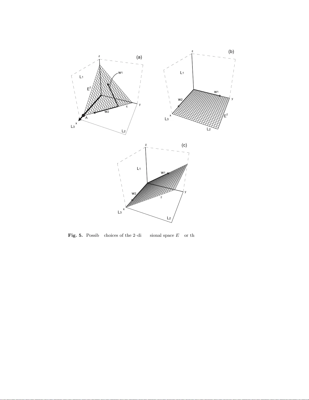
The Ly apuno v Characteristic Exp onen ts and their computation Charalamp os Skok os 12 1 Astronomie et Syst` emes Dynamiques, IMCCE, Observ atoire de Paris, 77 av enue Denfert–Rochereau, F-75014, Pari s, F ra n ce 2 Max Planc k Institute for the Physics of Complex Systems, N¨ othnitzer Strasse 38, D-01187, Dresden, Germany hskokos@pk s.mpg.de F or wan t of a nail the sho e was lost. F or want of a sho e the horse was lost. F or wan t of a horse the rider was lost. F or wan t of a rider the b attle was lost. F or wan t of a b attle the kingdom was lost. An d al l for the want of a horses ho e nail. F or Want of a Nail (prov erbial rhyme) Summary . W e present a survey of the theo ry o f the Ly apu nov Characteri st ic Exp o- nents (LCEs) for dyn amical systems, as well as o f the numerical tec hniqu es developed for the computation of the maximal, of few and of all of them. A fter some histor- ical notes on the ﬁrst attempts for the numeric al ev aluation of LCE s, w e discuss in detail the m u ltiplicativ e ergo dic theorem of Osel edec [102], which provides the theoretical basis for the computation of th e LCEs. Then, we analyze the algorithm for the compu t ation o f the maximal LC E, whose v alue has b een extensivel y used as an indicator of c haos, and the algorithm of the so–called ‘standard method ’, devel- oped by Benettin et al. [14], for the computation of man y LCEs. W e also consider diﬀerent discrete and contin uous methods for computing the LCEs based on the QR or the singular v alue decomp osition techniques. Although, we are mainly interested in ﬁnite–dimensional conserv ativ e systems, i. e. autonomous Hamiltonian systems and symplectic maps, we also brieﬂy refer t o the ev aluation of LCEs of dissipativ e systems and time series. The relation of tw o chaos detection tec h niques, namely the fast Lyapuno v ind icator (FLI) and the generalized alig nment index ( GALI), to the computation of the LCEs is also d iscussed. Key words: Lyapuno v exp onents; Multiplica tive ergo dic t h eorem; Numerical tech- niques; Dynamical systems; Chaos; V ariational equations; T angen t map; Chaos de- tection metho ds 1 In tro duction . . . . . . . . . . . . . . . . . . . . . . . . . . . . . . . . . . . . . . . . . . . . . . 2 2 Ch. Skok os 2 Autonomous Hamiltoni an system s and sym pl ectic maps . . . 7 2.1 V ariational equations and tangent map . . . . . . . . . . . . . . . . . . . . . . . . . 8 2.2 Simple examples o f dynamical s y stems . . . . . . . . . . . . . . . . . . . . . . . . . 9 2.3 Numerical in tegra tion of v ariationa l equations . . . . . . . . . . . . . . . . . . . 10 2.4 T angent dynamics of symplectic maps . . . . . . . . . . . . . . . . . . . . . . . . . . 11 3 Historical in tro duction: The early da ys of LCEs . . . . . . . . . . . 12 4 Ly apuno v Chara cteristi c Exp onent s: Theoretical treatment 14 4.1 Deﬁnitions and basic theorems . . . . . . . . . . . . . . . . . . . . . . . . . . . . . . . . 16 4.2 Computing LCEs of or der 1 . . . . . . . . . . . . . . . . . . . . . . . . . . . . . . . . . . 20 4.3 Computing LCEs of or der p > 1 . . . . . . . . . . . . . . . . . . . . . . . . . . . . . . . 22 4.4 The Multiplicativ e Ergo dic Theorem . . . . . . . . . . . . . . . . . . . . . . . . . . . 24 4.5 Prop erties of the sp ectrum of LCEs . . . . . . . . . . . . . . . . . . . . . . . . . . . . 28 5 The maximal LCE . . . . . . . . . . . . . . . . . . . . . . . . . . . . . . . . . . . . . . . . 30 5.1 Computation of the mLCE . . . . . . . . . . . . . . . . . . . . . . . . . . . . . . . . . . . 30 5.2 The n umer ica l algo rithm . . . . . . . . . . . . . . . . . . . . . . . . . . . . . . . . . . . . . 32 5.3 Behavior of X 1 ( t ) for re g ular a nd c ha otic orbits . . . . . . . . . . . . . . . . . 34 6 Computation of the sp e ctrum of LCEs . . . . . . . . . . . . . . . . . . . . 36 6.1 The standard metho d for computing LCEs . . . . . . . . . . . . . . . . . . . . . 38 6.2 The n umer ica l algo rithm for the standard metho d . . . . . . . . . . . . . . . 43 6.3 Connection betw ee n the sta nda rd metho d and the QR decomp osition . . . . . . . . . . . . . . . . . . . . . . . . . . . . . . . . . . . . . . . . . . . . . . 44 6.4 Other methods for computing LCEs . . . . . . . . . . . . . . . . . . . . . . . . . . . 47 Contin uous QR decomp os ition metho ds . . . . . . . . . . . . . . . . . . . . . . . . . . . . . 50 Computing the complete sp ectrum of LCEs . . . . . . . . . . . . . . . . . . . . . . . . . 51 Computation of the p > 1 larg est LCEs . . . . . . . . . . . . . . . . . . . . . . . . . . . . . 52 Discrete a nd conti n uo us metho ds based on the SVD pro ce dur e . . . . . . . . . 53 7 Chaos detection tec hniques . . . . . . . . . . . . . . . . . . . . . . . . . . . . . . . 54 8 LCEs of dissipative systems and tim e series . . . . . . . . . . . . . . . 58 8.1 Dissipative systems . . . . . . . . . . . . . . . . . . . . . . . . . . . . . . . . . . . . . . . . . . 5 9 8.2 Computing LCEs fro m a time series . . . . . . . . . . . . . . . . . . . . . . . . . . . 59 A Exterior algebra and w e dg e pro duct: Some basic notions . . 62 A.1 An illustrativ e example . . . . . . . . . . . . . . . . . . . . . . . . . . . . . . . . . . . . . . 66 References . . . . . . . . . . . . . . . . . . . . . . . . . . . . . . . . . . . . . . . . . . . . . . . . . . . . . 68 1 In tro duction One o f the basic information in understanding the behavior of a dynamical system is the knowledge of the sp ectrum of its Lyapunov Char acteristic Exp o- Lyapuno v Characteristic Exp onents 3 nents (LCEs) . The LCE s ar e asy mptotic meas ures characterizing the a verage rate of growth (or shr inking ) of small p erturbations to the solutions of a dy- namical system. Their concept w as in tro duced by Lyapuno v when studying the stability of nonstationary solutions of o r dinary diﬀeren tial equa tio ns [9 6], and has b een widely employ ed in studying dynamica l s ystems since then. The v alue of the maxima l LCE (mLCE) is an indicator of the chaotic or regu- lar nature of orbits, while the whole spectrum of LCEs is re la ted to en tropy (Kolmogor ov–Sinai en tropy) and dimension– like (Lyapunov dimension) quan- tities that characterize the underlying dynamics. By dynamic al system we refer to a ph ysica l and/or mathematical system consisting of a) a set of l rea l state v ariables x 1 , x 2 . . . , x l , whose curre nt v alues deﬁne the state of the system, and b) a w e ll–deﬁned rule from which the evolution of the sta te with respect to an indep endent real v ariable (whic h is usually referred as the time t ) can be derived. W e refer to the n umber l of state v ariables a s the dimension of the system, and denote a s tate using the vector x = ( x 1 , x 2 . . . , x l ), or the matrix x = [ x 1 x 2 . . . x l ] T notation, where ( T ) deno tes the tra ns p o s e matrix. A particular state x corr esp onds to a po in t in a n l – dimensional space S , the so–called phase sp ac e of the system, while a set of states x ( t ) parameterized by t is r eferred as a n orbit of the dyna mica l system. Dynamical systems come in essentially tw o types : 1. Continuous dynamic al systems des crib ed by diﬀerential equations of the form ˙ x = d x dt = f ( x , t ) , with dot denoting der iv ativ e with resp ect to a co n tinuous time t and f being a set of l functions f 1 , f 2 . . . , f l known as the ve ct or ﬁeld . 2. Discr ete dynamic al systems or maps , descr ib ed b y diﬀerence equations o f the form x n +1 = f ( x n ) , with f b eing a set of l functions f 1 , f 2 . . . , f l and x n denoting the vector x at a discr e te time t = n (in teger). Let us now deﬁne the ter m chaos . In the literature there are man y deﬁni- tions. A brief and concise pre s ent a tion o f them can be found for exa mple in [90]. W e adopt here one of the most famous deﬁnitions of c hao s due to De- v aney [3 5, p. 50], which is based on the top ologica l approach of the pro blem. Deﬁnition 1. L et V b e a set and f : V → V a map on this set. We say that f is chaotic on V if 1. f has sensitive dep endenc e on initial c onditions. 2. f is top olo gic al ly tr ansitive. 3. p erio dic p oints ar e dense in V . 4 Ch. Skok os Let us expla in in more detail the hypo thesis o f this deﬁnition. Deﬁnition 2. f : V → V has sen sitiv e d epende nce on init ial condi tions if ther e exists δ > 0 such that, for any x ∈ V and any neighb orho o d ∆ of x , ther e exist y ∈ ∆ and n ≥ 0 , such that | f n ( x ) − f n ( y ) | > δ , wher e f n denotes n su c c essive applic ations of f . Practically this deﬁnition implies that there exist points arbitrarily close to x whic h even tually s eparate from x b y at least δ under iterations of f . W e po in t out that no t all p oints nea r x need even tually mov e aw ay fro m x under iteration, but there must b e at lea s t one such p oint in every neighborho o d of x . Deﬁnition 3. f : V → V is said to b e topol ogica lly t ransit ive if for any p air of op en sets U, W ⊂ V ther e exists n > 0 such that f n ( U ) ∩ W 6 = ∅ . This deﬁnitions implies the e x istence of points which ev ent ua lly move under iteration from one arbitrar ily small neighbo r ho o d to any o ther. Consequently , the dynamical system cannot b e decompose d into tw o dis jo in t in v aria nt o pen sets. F rom Deﬁnition 1 we see that a chaotic sys tem p osses ses three ingredients: a) unpredictability becaus e of the s e nsitiv e dep endence on initial conditions, b) indecomposa bilit y , b ecaus e it cannot be decomp osed int o nonin terac ting subsystems due to top olog ical transitivity , and c) an element of r egularity beca use it has p erio dic p oints which ar e dense. Usually , in physics and applied sciences, people fo cus on the ﬁrst hypo th- esis of Deﬁnition 1 and use the notion of chaos in relation to the sensitiv e dependence on initial conditions. The mo s t commo nly employ e d metho d for distinguishing betw e e n regular and c haotic motion, which quantiﬁes the s en- sitive dependence on initial conditions, is the ev a luation of the mLCE χ 1 . If χ 1 > 0 the o rbit is chaotic. This metho d was initially dev e lo pe d at the late 70’s based on theoretica l r esults o btained a t the end of the 60’s. The concept of the LCEs has bee n widely presented in the litera ture from a practical po int of view, i. e. the descr iption of particular num e r ical algorithms for their computation [54, 44, 62, 92, 36]. Of course, there also exist theoret- ical studies on the LCEs, which are mainly fo cused on the pro blem of their existence, starting with the pioneer work of Oseledec [102]. In that pap er the Multiplicativ e E rgo dic T heo rem (MET), which provided the theoretical ba sis for the numerical computation o f the LCEs, was stated and prov ed. The MET was the sub ject of several theoretical studies afterwards [108, 1 14, 76, 1 41]. A combination of impor tant theoretical and numerical results on LCEs can b e found in the seminal pap ers of Benettin et al. [13, 14], written almost 30 years ago, where an ex plicit method for the computation of a ll LCEs was developed. In the prese n t rep ort we fo cus our atten tion b oth on the theoretical fr a me- work of the LCEs , as well as on the numerical techniques developed for their computation. Our goal is to pr ovide a survey of the basic r esults on these issues obtained o ver the last 40 years, after the work o f Oseledec [102]. T o Lyapuno v Characteristic Exp onents 5 this end, w e present in detail the mathematical theory of the L CEs and dis- cuss its sig niﬁca nce without going through tedio us mathematical proo fs. In our a pproach, we prefer to pre s ent the deﬁnitions o f v ario us quantit ies a nd to state the basic theorems that guarantee the existence of the LCE , citing a t the same time the paper s where all the related mathematical pro ofs can b e found. W e also describ e in detail the v ar ious numerical techniques dev elo ped for the ev aluation of the maxima l, of few or even of all LCE s, and e xplain their prac tica l implemen tation. W e do not restrict our prese ntation to the so– called standar d metho d developed by Benettin et a l. [14], as it is usua lly do ne in the literature (see e. g. [54, 44, 92 ]), but w e include in our study mo dern tech niques for the computation of the LCEs like the discrete and contin u- ous methods based on the singular v alue decomp osition (SVD) and the QR decomp osition pro cedures. In our a nalysis we deal with ﬁnite–dimensional dynamica l systems and in particular with autonomous Hamiltonian systems and symplectic maps deﬁned on a c ompact manifold, mea ning that w e exclude cases with escap es in which the mo tion ca n g o to inﬁnit y . W e do no t co ns ider the rather exce ptional cases of completely c ha otic systems and of in tegra ble o nes, i. e. systems that can b e solved explicitly to g ive their v a riables as single– v alued functions of time, but we consider the most genera l case of ‘systems with divided phase space’ [30, p. 19] for which r e gular 1 (quasip erio dic) and chaotic orbits co – exist. In suc h systems one sees b o th regular a nd chaotic do mains. B ut the regular domains contain a dense set of unstable p erio dic orbits, which are followed by small c hao tic regio ns . On the other hand, the c haotic domains contain s table per io dic orbits that ar e follow ed by small islands of stability . Th us, the reg ular and ch aotic domains are intricately mixed. How ever, there are regions where order is predominan t, and other r egions wher e c hao s is predominant. Although in our rep ort the theor y o f LCEs and the numerical tec hniques for their ev aluation a re pres ent ed mainly for c onservative systems , i.e. system that pres erve the phase space volume, these techn iq ues are not v alid only for such mo dels. F o r completeness sake, w e also brieﬂy discuss at the end of the rep ort the computation of LCEs for dissip ative systems , for which the phase space v o lume decr eases o n average, and fo r time series. W e tr ied to make the paper self–consis tent by including deﬁnitions of the used terminolo gy and brief ov erv ie ws o f all the necessa ry mathematical no - tions. In addition, whenever it was considered necess ary , some illustrative examples ha ve been added to the text in o rder to cla r ify the practical imple- men ta tion of the presen ted material. Our aim has be e n to make this r eview of use for b oth the novice and the more exp erienced practitioner interested in LCE s . T o this end, the reader who is in ter ested in rea ding up on detailed tech nica lities is pr ovided with numerous signp osts to the r elev ant litera ture. Throughout the text bold low erca se letters denote vectors, while matri- ces are represented, in general, b y capital b old letters. W e also note that the 1 Regular orbits are often called or der e d orbits (see e. g. [30, p. 18]). 6 Ch. Skok os most frequentl y used abbreviations in the text are: LCE(s), Lyapuno v Char- acteristic Expo nent (s); p –LCE, Ly a punov Characteristic Exponent of order p ; mLCE , max ima l Lyapuno v Character istic Exp o nent ; p –mLCE , maximal Lyapuno v Characteristic Expo nent of order p ; MET, mult iplicative er g o dic theorem; SVD, Singula r V alue Decomp osition; PSS, P o incar´ e s ur face of sec- tion; FLI, fast Lyapunov indicator ; GALI, generalized alignmen t index. The pa per is org anized as follows: In Section 2 we pr esent the ba sic concepts of Hamiltonian s y stems and symplectic maps, empha s izing on the evolution of orbits, as well a s o f deviation vectors ab out them. In particular, w e deﬁne the so–ca lled v aria tional equatio ns for Hamiltonian systems and the tangent map for symplectic maps, which gov ern the time evolution of deviation vectors. W e also provide some s imple examples of dynamical systems and derive the corr e s po nding set of v aria tional equations and the cor r esp onding tang e nt map. Section 3 contains some historical notes o n the ﬁrst attempts for the appli- cation of the theoretical results of Oseledec [102] for the actual computation of the LCEs. W e recall how the notion of exp onential divergence of nearby orbits was even tually quant iﬁed b y the co mputation of the mLCE, and w e refer to the pap ers where the mLCE or the sp ectrum o f LCE s were computed for the ﬁr s t time. The basic theoretical results on the LCEs are pres en ted in Section 4 follow- ing mainly the milesto ne pap ers of Oseledec [102] and Benettin et al. [13, 14]. In Section 4.1 the basic deﬁnitions and theoretical results of LCEs of v a rious orders ar e presented. The practical conseq uence s o f these results on the com- putation of the LCEs of order 1 and of order p > 1 are discussed in Sections 4.2 and 4.3 respectively . Then, in Section 4.4 the MET of Oseledec [102 ] is stated in its v ario us for ms, while its conse q uences on the spec tr um of LCE s for conserv ative dynamica l sy stems a re discussed in Section 4.5. Section 5 is devoted to the computation of the mLCE χ 1 , which is the oldest chaos indicator used in the liter ature. In Section 5.1 the method for the computation of the mLCE is discussed in gr eat detail a nd the theor etical basis of its ev aluation is explained. The corresp onding a lgorithm is presented in Section 5.2, while the b ehavior o f χ 1 for regular and chaotic or bits is analyzed in Section 5.3 . In Section 6 the v ar ious methods fo r the computation of part or of the whole sp ectrum o f LCEs ar e presented. In particular , in Section 6.1 the stan- dard metho d developed in [119, 1 4], is presented in g r eat detail, while the corresp onding algo r ithm is given in Section 6.2. In Section 6.3 the co nnec- tion of the standard method with the discrete QR decomp osition technique is discussed and the co r resp onding Q R algorithm is g iven, while Section 6.4 is devoted to the presen tatio n of other tec hniques for computing few o r all LCEs, whic h are based on the SVD and QR decompo sition algorithms. In Section 7 we brieﬂy refer to v a r ious chaos detection tec hniques bas ed on the ana lysis of deviation v ector s, as well as to a second ca tegory of chaos indicators ba sed on the analysis of the time series constructed by the co ordi- Lyapuno v Characteristic Exp onents 7 nates of the orbit under consideration. The r elation of tw o c ha o s indicators, namely the fast Ly apunov indicator (FLI) and the generalized alignmen t index (GALI), to the computation of the LCEs is also discussed. Although the main to pic of o ur presentation is the theory and the com- putation of the LCE s for conserv ative dynamical systems, in the las t section of o ur rep or t some complement ary is s ues rela ted to other t yp es of dynamical systems are concisely presented. In particular, Section 8.1 is devoted to the computation of the LCEs for diss ipative s ystems, while in Section 8.2 some basic features on the numerical computation of the LCEs fr om a time s e r ies are presented. Finally , in the appendix A w e present s ome basic elements of the exterior algebra theor y in connection to the ev aluation of wedge pro ducts, which ar e needed for the computation of the volume elements appear ing in the deﬁni- tions o f the v ar ious LCE s. 2 Autonomous Hamiltonian systems and symplectic maps In our study we co nsider tw o main types of conserv ative dynamical systems: 1. Contin uous systems corresp onding to a n autonomous Hamiltonian system of N degrees ( N D) of freedom having a Hamiltonian function H ( q 1 , q 2 , . . . , q N , p 1 , p 2 , . . . , p N ) = h = constant , (1) where q i and p i , i = 1 , 2 , . . . , N are the gener a lized co ordinates and con- jugate mo men ta resp ectively . An orbit in the l = 2 N – dimensional phase space S o f this system is deﬁned by a vector x ( t ) = ( q 1 ( t ) , q 2 ( t ) , . . . , q N ( t ) , p 1 ( t ) , p 2 ( t ) , . . . , p N ( t )) , with x i = q i , x i + N = p i , i = 1 , 2 , . . . , N . The time evolution of this or bit is gov e r ned by the Hamilton equations of motion, whic h in matrix form are given by ˙ x = f ( x ) = h ∂ H ∂ p − ∂ H ∂ q i T = J 2 N · DH , (2) with q = ( q 1 ( t ) , q 2 ( t ) , . . . , q N ( t )), p = ( p 1 ( t ) , p 2 ( t ) , . . . , p N ( t )), a nd DH = h ∂ H ∂ q 1 ∂ H ∂ q 2 · · · ∂ H ∂ q N ∂ H ∂ p 1 ∂ H ∂ p 2 · · · ∂ H ∂ p N i T . Matrix J 2 N has the following block for m J 2 N =  0 N I N − I N 0 N  , 8 Ch. Skok os with I N being the N × N ident ity matrix and 0 N being the N × N matrix with all its element s equal to zero. The s olution of (2) is formally written with respec t to the induced ﬂow Φ t : S → S as x ( t ) = Φ t ( x (0)) . (3) 2. Symplectic maps o f l = 2 N dimensions having the form x n +1 = f ( x n ) . (4) A symple ctic map is an area–pre s erving map whose Jac obia n matrix M = Df ( x ) = ∂ f ∂ x =       ∂ f 1 ∂ x 1 ∂ f 1 ∂ x 2 · · · ∂ f 1 ∂ x 2 N ∂ f 2 ∂ x 1 ∂ f 2 ∂ x 2 · · · ∂ f 2 ∂ x 2 N . . . . . . . . . ∂ f 2 N ∂ x 1 ∂ f 2 N ∂ x 2 · · · ∂ f 2 N ∂ x 2 N       , satisﬁes M T · J 2 N · M = J 2 N . (5) The state o f the sy stem a t the discr ete time t = n is given b y x n = Φ n ( x 0 ) = ( f ) n ( x 0 ) , (6) where ( f ) n ( x 0 ) = f ( f ( · · · f ( x 0 ) · · · )), n times. 2.1 V ariational equations and tangen t map Let us now turn our atten tion to the (contin uous or disc rete) time evolution of deviation v ector s w from a given reference orbit of a dyna mical system. These vectors evolv e on the tangent sp ac e T x S of S . W e deno te by d x Φ t the linear mapping which maps the tangent space of S at p oint x onto the tangent space at p oint Φ t ( x ), a nd so we have d x Φ t : T x S → T Φ t ( x ) S w ith w ( t ) = d x Φ t w (0) , (7) where w (0), w ( t ) are deviation vectors with resp ect to the given orbit at times t = 0 and t > 0 respectively . In th e case of the H a miltonian system (1) an in itial deviation vector w (0) = ( δ x 1 (0) , δ x 2 (0) , . . . , δ x 2 N (0)) from the solution x ( t ) (3) ev o lves on the tangent spa ce T x S a ccording to the so–ca lled variational e quations ˙ w = Df ( x ( t )) · w = ∂ f ∂ x ( x ( t )) · w =  J 2 N · D 2 H ( x ( t ))  · w =: A ( t ) · w , (8) with D 2 H ( x ( t )) b eing the Hessian ma trix of Hamiltonian (1) calc ula ted on the reference orbit x ( t ) (3), i. e. Lyapuno v Characteristic Exp onents 9 D 2 H ( x ( t )) i,j = ∂ 2 H ∂ x i ∂ x j     Φ t ( x (0)) , i, j = 1 , 2 , . . . , 2 N . W e underline that equations (8) r epresent a set o f line ar diﬀer ential e quations with resp ect to w , having time dependent co eﬃcients since, matrix A ( t ) de- pends on the particular r eference orbit, which is a function of time t . The solution of (8) can b e written a s w ( t ) = Y ( t ) · w (0) , (9) where Y ( t ) is the so –called fun damental matrix of solutions o f (8), satisfying the equation ˙ Y ( t ) = Df ( x ( t )) · Y ( t ) = A ( t ) · Y ( t ) , with Y (0) = I 2 N . (10) In the case of the symplectic ma p (4) the evolution of a deviation vector w n , with r esp ect to a refere nce orbit x n , is given b y the corr esp onding tangent map w n +1 = Df ( x n ) · w n = ∂ f ∂ x ( x n ) · w n =: M n · w n . (11) Thu s , the evolution of the initial deviation v e c to r w 0 is given by w n = M n − 1 · M n − 2 · . . . · M 0 · w 0 =: Y n · w 0 , (12) with Y n satisfying the r elation Y n +1 = M n · Y n = Df ( x n ) · Y n , with Y 0 = I 2 N . (13) 2.2 Simpl e e xampl e s of dynamical systems As representativ e examples of dynamical systems we co nsider a) the w ell– known 2D H ´ enon–Heiles system [72], having the Hamiltonian function H 2 = 1 2 ( p 2 x + p 2 y ) + 1 2 ( x 2 + y 2 ) + x 2 y − 1 3 y 3 , (14) with equations o f motio n ˙ x =     ˙ x ˙ y ˙ p x ˙ p y     = J 4 · D H 2 = J 4 ·     x + 2 xy y + x 2 − y 2 p x p y     ⇒        ˙ x = p x ˙ y = p y ˙ p x = − x − 2 xy ˙ p y = − y − x 2 + y 2 , (15) and b) the 4– dimensional (4d) symplectic map x 1 ,n +1 = x 1 ,n + x 3 ,n x 2 ,n +1 = x 2 ,n + x 4 ,n x 3 ,n +1 = x 3 ,n − ν sin( x 1 ,n +1 ) − µ [1 − cos( x 1 ,n +1 + x 2 ,n +1 )] x 4 ,n +1 = x 4 ,n − κ sin( x 2 ,n +1 ) − µ [1 − cos( x 1 ,n +1 + x 2 ,n +1 )] (mod 2 π ) , (16) with parameter s ν , κ and µ . All v ar iables are g iven (mo d 2 π ), so x i,n ∈ [ π , π ), for i = 1 , 2 , 3 , 4. This map is a v ar ia nt of F ro eschl ´ e’s 4d symplectic map [52] and its behavior has be e n studied in [31, 123]. It is easily seen that its Jacobian matrix satisﬁes e q uation (5). 10 Ch. Skok os 2.3 Numerical integration of v ariational equations When dealing with Ha miltonia n systems the v ariational equations (8) hav e to be integrated simult a neously with the Hamilton equations of motion (2). Let us clarify the issue by lo oking to a s peciﬁc ex ample. The v ariational e q uations of the 2D Hamiltonian (14) are ˙ w =     ˙ δ x ˙ δ y ˙ δ p x ˙ δ p y     =     0 0 1 0 0 0 0 1 − 1 − 2 y − 2 x 0 0 − 2 x − 1 + 2 y 0 0     ·     δ x δ y δ p x δ p y     ⇒        ˙ δ x = δ p x ˙ δ y = δ p y ˙ δ p x = ( − 1 − 2 y ) δ x + ( − 2 x ) δy ˙ δ p y = ( − 2 x ) δ x + ( − 1 + 2 y ) δ y . (17) This sys tem of diﬀerential equations is linea r with resp ect to δ x , δ y , δ p x , δ p y , but it ca nno t b e in tegra ted indep endently of system (15) since the x and y v ariables appea r explicitly in it. Thus, if w e w ant to follow the time evolution o f an initial dev iation v ector w (0) with resp ect to a reference o r bit with initial condition x (0), w e ar e obliged to integrate simultaneously the whole set o f diﬀerential equations (15) and (17). A n umerica l sc heme for in tegrating the v a riational equations (8), whic h exploits their linearity a nd is particular ly useful when we need to evolv e more than one devia tio n vectors is the following. Solving the Ha milton equations of motion (2) b y any numerical integration scheme we obtain the time evolution of the re ference o rbit (3 ). In pra c tice this means that we know the v alues x ( t i ) for t i = i ∆t , i = 0 , 1 , 2 , . . . , wher e ∆t is the in tegr ation time step. Inserting this n umerically kno wn solution to the v ariational equations (8) we end up with a linear system of diﬀerential equations with constant co eﬃcients for every time in terv al [ t i , t i + ∆t ) , which can b e solved explicitly . F or example, in the pa rticular ca se of Hamiltonian (14), the system of v ariational equations (17) b ecomes ˙ δ x = δ p x ˙ δ y = δ p y ˙ δ p x = [ − 1 − 2 y ( t i )] δ x + [ − 2 x ( t i )] δ y ˙ δ p y = [ − 2 x ( t i )] δ x + [ − 1 + 2 y ( t i )] δ y , for t ∈ [ t i , t i + ∆t ) , (18) which is a linear system of diﬀerent ia l equa tions with constant co eﬃcients and th us, easily so lved. In particular, equa tions (18 ) ca n by co ns ider ed as the Hamilton equations of motion corres p o nding to the Hamiltonian function H V ( δ x, δ y , δ p x , δ p y ) = 1 2  δ p 2 x + δp 2 y  + 1 2  [1 + 2 y ( t i )] δ x 2 + [1 − 2 y ( t i )] δ y 2 + 2 [2 x ( t i )] δ xδ y  . (19) Lyapuno v Characteristic Exp onents 1 1 The Hamiltonian formalism (19) of the v ar iational equations (18) is a sp e c iﬁc e x ample o f a mo re general r esult. In the case of the usual Hamiltonian function H ( q , p ) = 1 2 N X i =1 p 2 i + V ( q ) , (20) with V ( q ) b eing the po ten tia l function, the v ariationa l equa tions (8) for the time in terv al [ t i , t i + ∆t ) take the form (see e. g. [12]) ˙ w =  ˙ δ q ˙ δ p  =  0 N I N − D 2 V ( q ( t i )) 0 N  ·  δ q δ p  with δ q = ( δ q 1 ( t ) , δ q 2 ( t ) , . . . , δ q N ( t )), δ p = ( δ p 1 ( t ) , δ p 2 ( t ) . . . , δ p N ( t )), a nd D 2 V ( q ( t i )) j k = ∂ 2 V ( q ) ∂ q j ∂ q k     q ( t i ) , j, k = 1 , 2 , . . . , N . Thu s , the tangen t dynamics of (20) is represented by the Hamiltonian fun c tio n (see e. g . [1 0 5]) H V ( δ q , δ p ) = 1 2 N X j =1 δ p 2 i + 1 2 N X j,k D 2 V ( q ( t i )) j k δ q j δ q k . 2.4 T angen t dynamics of symplectic m aps In the case of symplectic ma ps, the dynamics on the tangent space, which is describ ed by the tang ent map (11), ca nnot be considered separately fro m the phase space dynamics determined by the map (4) itself. This is b ecause the tangent map depends explicitly on the reference or bit x n . F or example, the tange nt map of the 4d map (16) is δ x 1 ,n +1 = δ x 1 ,n + δx 3 ,n δ x 2 ,n +1 = δ x 2 ,n + δx 4 ,n δ x 3 ,n +1 = a n δ x 1 ,n + b n δ x 2 ,n + ( 1 + a n ) δ x 3 ,n + b n δ x 4 ,n δ x 4 ,n +1 = b n δ x 1 ,n + c n δ x 2 ,n + b n δ x 3 ,n + ( 1 + c n ) δ x 4 ,n , (21) with a n = − ν cos( x 1 ,n +1 ) − µ sin( x 1 ,n +1 + x 2 ,n +1 ) b n = − µ sin( x 1 ,n +1 + x 2 ,n +1 ) c n = − κ cos( x 2 ,n +1 ) − µ sin( x 1 ,n +1 + x 2 ,n +1 ) , which explicitly dep end on x 1 ,n , x 2 ,n , x 3 ,n , x 4 ,n . Thus, the evoluti on of a deviation vector requires the simultaneous iteration of bo th the map (16) and the tangent map (21). 12 Ch. Skok os 3 Historical in tro duction: The early da ys of LCEs Prior to the discussion of the theory of the LCEs and the presentation of the v arious algorithms for their computation, it would b e in teresting to g o bac k in time and see how the notion of LCEs, a s well as the now adays ta ken for granted techniques for ev a luating them, were for med. The LCEs a re as ymptotic measures characterizing the average ra te of growth (or shrinking) of small perturbations to the orbits of a dynamical system, and their concept was introduced by Ly apunov [96]. Since then they hav e b een extensively us ed for studying dynamica l systems. As it has alrea dy been mentioned, one o f the basic features o f chaos is the sensitive dependence on initial co nditions and the LCEs provide quantitativ e measures o f resp onse sensitivit y of a dynamical system to small changes in initial c o nditions. F or a chaotic orbit a t least one LCE is p ositive, implying exp onential divergence o f nearby o rbits, while in the case o f regula r orbits all LCE s are ze ro. Ther efore, the presence of p os itive LCEs is a signa ture of chaotic b ehavior. Usually the computation of only the mLCE χ 1 is suﬃcien t for determining the nature of an orbit, because χ 1 > 0 guarantees that the orbit is c ha otic. Characteriza tion o f the chaoticity of an or bit in terms of the divergence of nearb y orbits was introduced b y H ´ enon and Heiles [72] and further used b y several authors (e. g . [48, 51, 52, 131, 22, 21]). In these studies tw o initial po in ts were chosen v e r y close to eac h other, ha v ing phase spa ce distance of ab out 10 − 7 − 10 − 6 , and were evolv ed in time. If the t wo initial p o int s were lo cated in a region of regula r motion their distance increased approximately linearly with time, while if they w ere b elonging to a chaotic reg ion the distance exhibited an exp onential increase in time (Figure 1). Although the theory of LCEs was applied to characterize ch aotic motion b y Oseledec [102], quite some time pa ssed until the co nnection b etw een LCE s and ex po nen tial divergence was made clear [10, 106]. It is worth mentioning that Casa rtelli et al. [21] deﬁned a quantit y , whic h they called ‘sto chastic parameter’, in order to qua n tify the exponential div er gence of nearby orbits, which w a s realized afterwards in [10] to be an estimator of the mLCE for t → ∞ . So, the mLCE χ 1 was estimated for the ﬁrst time in [10], a s the limit for t → ∞ o f an appropriate qua n tity X 1 ( t ), whic h was o btained from the evolution of the phase space distance of tw o initially clo se orbits. In this pap er some no wadays well–established properties of X 1 ( t ) were discussed, like for example the fact that X 1 ( t ) tends to zero in the ca s e of regular orbits following a p ower law ∝ t − 1 , while it tends to nonzero v alues in the case of c ha otic orbits (Figure 2). The sa me algorithm was immediately applied fo r the c o mputation of the mLCE of a dissipative s ystem, namely the Lor enz s ystem [9 9]. The next impro vemen t of the computational algor ithm for the ev aluation of the mLCE was in tro duced in [34], where the v ar iational equations w ere used for the time evolution of deviation v e c to rs instead of the previous appr oach of the simultaneous in tegr ation of t wo initially close orbits. This more dir e c t Lyapuno v Characteristic Exp onents 1 3 Fig. 1. Typical b ehavior of the t ime evolution of th e distance D b etw een tw o initially close orbits in the case of regular and chao tic orbits. The particular results are obtained for a 2D Hamiltonian system describing a T o d a lattice of tw o particles with un eq ual masses (see [22] for more details). The initial Euclidian d istance of the tw o orbits in the 4–dimensional phase space is D 0 = 10 − 6 . D exhibits a linear (on the av erage) gro wth when the t wo orbits are initially lo cated in a regio n of regular motion (left panel), while it gro ws exp onentially in t he case of chaotic orbits (righ t panel). The big diﬀerence in th e val u es of D b et w een the tw o cases is ev ident since the tw o panels ha ve the same horizon tal (time) axis but d iﬀerent vertical ones. In particular, the vertica l axis is linear in the left panel and log arithmic in the righ t panel (after [22]). approach c onstituted a signiﬁcant improvem ent for the co mputation of the mLCE since it allowed the use of larger int egration steps, diminishing the real computational time and also eliminated the problem o f c ho o sing a suitable initial distance b etw een the nearby orbits. In [11] a theorem was formulated, which led directly to the dev elo pment of a n umerical tec hnique for the computation of some or even of all LCEs, based on the time evolution o f mor e than o ne deviation vectors, whic h are kept linearly indep endent thro ugh a Gram–Schmidt orthonorma lization pro cedure (see also [9]). This metho d was explained in more detail in [11 9], where it was applied to the study o f the Lor enz system and w as also pr esented in [1 2], where it was applied to the s tudy of an N D Hamiltonian system with N v arying fro m 2 to 10. The theoretical framework, as well a s the n umerica l method for the co m- putation of the maxima l, some or even all LCEs w er e giv en in the semina l pap ers of Benettin et a l. [13, 14]. In [14] the complete set of LCEs was cal- culated for several diﬀeren t Hamiltonia n systems, including four and six di- mensional maps. In Figure 3 w e sho w the results of [14] concerning the 3D Hamiltonian s ystem o f [34]. The impor tance of the pa pe r s of Benettin et a l. [13, 14] is reﬂected by the fact that almost all metho ds for the computation o f the LCE s ar e more or less based o n them. Immediately the ideas presented in 14 Ch. Skok os Fig. 2. Evolution of X 1 ( t ) (denoted as k n ) with respect to time t (denoted by n × τ ) in log–log scale for several orbits of the H´ enon–Heiles system (14). In the left p anel X 1 ( t ) is computed for 5 diﬀeren t regular orbits at diﬀeren t energies H 2 (denoted as E ) and it tends to zero follo wing a p ow er la w ∝ t − 1 . A dashed straigh t line corresponding to a function p roportional to t − 1 is also p lotted. I n the righ t panel the evolutio n of X 1 ( t ) is plotted for three regular orbits (curves 1–3) and three chaotic ones (curves 4–6) for H 2 = 0 . 125. Note that the v alues of the initial conditions giv en in the tw o panels corresp ond to q 1 = x , q 2 = y , p 1 = p x , p 2 = p y in (14) (after [10]). [13, 1 4] were used for the computation o f the LCEs for a v ariety of dynamical systems lik e inﬁnite–dimensional systems describ ed b y delay diﬀerent ial equa- tions [4 6], dissipativ e systems [44], conserv ative systems related to Celestial Mechanics pr oblems [53, 5 5], as well as for the determination of the L CEs from a time ser ies [14 4, 11 8]. 4 Ly apuno v Characteristic Exponents: Theoretical treatmen t In this section we deﬁne the LCEs of v arious orders presenting als o the bas ic theorems whic h guarantee their existence a nd pro vide the theoretical back- ground for their numerical ev alua tion. In our presentation we basically follow the fundament a l pap ers of Os eledec [102] and of Benettin et a l. [1 3] where all the theoretical results of the current section are explicitly proved. W e consider a con tinuous or discr ete dyna mica l system deﬁned on a dif- ferent iable manifold S . Let Φ t ( x ) denote the s ta te at time t of the system which at time t = 0 was at x (see equations (3) and (6) for the cont in uo us and discrete case resp ectively). F or the action of Φ t ov er t wo successive time in ter v als t and s w e hav e the following comp osition law Φ t + s = Φ t ◦ Φ s . Lyapuno v Characteristic Exp onents 1 5 Fig. 3. Time evolution of appropriate quantiti es denoted by X ( t ) p , p = 1 , 2 , 3, h a v ing respectively as limits for t → ∞ the ﬁrst three LCEs χ 1 , χ 2 , χ 3 , for tw o chaotic orbits (left panel) and one regular orbit (right panel) of the 3D Hamiltonian system initially studied in [34] (see [14] for more details). In b oth panels X ( t ) 3 tends to zero implying that χ 3 = 0. This is du e to the fact that Hamiltonian systems h a ve at least one va n ishing LCE, namely the one corresp onding to the direction along the ﬂo w (this prop erty is ex plained in Section 4.5). On the other h an d, χ 1 and χ 2 seem to get nonzero v alues (with χ 1 > χ 2 ) for chao t ic orbits, while they app ear to vanis h for regular orbits (after [14]). The tangent space at x is mapp ed o n to the tange nt space at Φ t ( x ) by the diﬀerent ia l d x Φ t according to equation (7). The action of Φ t ( x ) is given by equation (9 ) for con tin uous systems and b y equation (12) for discrete ones . Thu s , the a c tio n of d x Φ t on a particular initial deviatio n vector w of the tangent space is given b y the multiplication of matrix Y ( t ) for contin uous systems or Y n for discrete systems with v ector w . F rom e q uations (9) and (12) w e see that the action o f d x Φ t ov er tw o successive time interv als t and s satisﬁes the c ompo sition la w d x Φ t + s = d Φ s ( x ) Φ t ◦ d x Φ s . (22) This equation can b e written in the form R ( t + s, x ) = R ( t, Φ s ( x )) · R ( s, x ) , (23) where R ( t, x ) is the matrix corresp onding to d x Φ t . W e no te that since Y (0) = Y 0 = I 2 N we get d x Φ 0 w = w and R (0 , x ) = I 2 N . A function R ( t, x ) satisfying relation (23) is called a mu ltiplic ative c o cycle with r esp ect to the dynamical system Φ t . 16 Ch. Skok os Let S be a mea sure spa ce with a normalized measure µ s uch that µ ( S ) = 1 , µ  Φ t A  = µ ( A ) (24) for A ⊂ S . Suppo se also that a smooth Riemannian metric k k is deﬁned on S . W e consider the multiplicativ e co cyc le R ( t, x ) co rresp onding to d x Φ t and we a re interested in its as ymptotic b ehavior for t → ±∞ . Since, as mentioned b y Oseledec [102], the case t → + ∞ is analogous to the case t → −∞ , we restrict our treatment to the ca se t → + ∞ , where time is increa sing. In order to cla rify what we are practically in teres ted in let us consider a nonzero vector w of the tangent space T x S a t x . Then the quantit y λ t ( x ) = k d x Φ t w k k w k is called the c o eﬃcient of exp ansion in the dir e ction of w . If lim s up t →∞ 1 t ln λ t ( x ) > 0 we say that exponential div er ge o ccurs in the direction o f w . Of cours e the basic question we hav e to a ns wer is whether the char acteristic exp onen t (also called char acteristic exp onent of or der 1 ) lim t →∞ 1 t ln λ t ( x ) exists. W e will answer this questio n in a more g eneral framework without re- stricting ours elves to mult iplica tiv e coc y cles. So, the res ults presented in the following Section 4.1, are v alid for a genera l class of matrix functions, a sub- class of which co ntains the multiplicativ e co cycles which a r e of mor e practical in ter est to us, since they describ e the time evolution of deviation vectors for the dynamical s y stems we s tudy . 4.1 Deﬁnitions and basic theorems Let A t be an n × n matrix function deﬁned either on the whole real axis or on the set of in teg ers, such that A 0 = I n , for each time t the v alue of function A t is a nonsingular matrix and k A t k the usual 2 –norm of A t 2 . In particular, we consider only ma trices A t satisfying 2 The 2– n orm k A k of an n × n matrix A is induced b y the 2–norm of v ectors, i. e. the usual Eu clidean norm k x k = ` P n i =1 x 2 i ´ 1 / 2 , by k A k = max x 6 =0 k Ax k k x k and is equal to the largest eigenv alue of matrix √ A T A . Lyapuno v Characteristic Exp onents 1 7 max  k A t k , k A − 1 t k  ≤ e ct (25) with c > 0 a suitable co ns tant . Deﬁnition 4. Considering a matrix function A t as ab ove and a nonzer o ve c- tor w of t he Euclidian sp ac e R n the quantity χ ( A t , w ) = lim sup t →∞ 1 t ln k A t w k (26) is c al le d the 1- dimens ional Lyapunov Charac terist ic Expo nent or t he Lyapun ov Charac teris tic E xponen t of order 1 (1-LCE ) of A t with re - sp e ct t o ve ctor w . F or simplicit y we will usually refer to 1 – LCEs a s LCEs. W e note that the v alue of the norm k w k does not inﬂuence the v alue of χ ( A t , w ). F or example, consider ing a vector β w , with β ∈ R a nonzero constant, instead of w in Deﬁnition 4, we get the extra term ln | β | /t (with | | denoting the a bs olute v alue) in eq ua tion (26) whose limiting v alue for t → ∞ is zero and thus does not change the v alue of χ ( A t , w ). Mor e importa n tly , the v alue of the LCE is independent of the norm a ppea ring in eq ua tion (26). This can b e easily seen as follows: Let us consider a se cond nor m k k ′ satisfying the inequalit y β 1 k w k ≤ k w k ′ ≤ β 2 k w k for some p os itiv e real num b ers β 1 , β 2 , and for a ll vectors w . Such norms are ca lled e qu ivalent (see e.g. [7 3, § 5.4.7 ]). Then, by the abov e – ment io ned argument it is easily seen that the use of norm k k ′ in (26) leav es unchanged the v a lue of χ ( A t , w ). Since all norms o f ﬁnite dimensiona l v ec tor spac e s are equiv alent , we conclude that the LCEs do not dep end on the chosen no r m. Let w i , i = 1 , 2 , . . . , p b e a set of linea rly indep endent vectors in R n , E p be the subspace genera ted b y all w i and vol p ( A t , E p ) b e the v olume of the p –parallelo gram ha ving as edg es the p vectors A t w i . This volume is computed as the norm of the w edge pro duct o f these vectors (see Appendix A for the deﬁnition of the wedge pro duct and the actual ev aluatio n of the v o lume) vol p ( A t , E p ) = k A t w 1 ∧ A t w 2 ∧ · · · ∧ A t w p k . Let a lso vol p ( A 0 , E p ) b e the volume of the initial p – pa rallelogr am deﬁned by all w i , since A 0 is the identit y matrix. Then the q uant it y λ t ( E p ) = vol p ( A t , E p ) vol p ( A 0 , E p ) is called the c o eﬃcient of exp ansion in t he dir e ction of E p and it depends only on E p and no t on the c hoice of the linear ly indep endent set of vectors. Obviously for an 1–dimensional subspace E 1 the coeﬃcient of expansion is k A t w 1 k / k w 1 k . If the limit 18 Ch. Skok os lim t →∞ 1 t ln λ t ( E p ) exits it is called the char acteristic exp onent of or der p in the dir e ction of E p . Deﬁnition 5. Considering the line arly indep endent set w i , i = 1 , 2 , . . . , p and the c orr esp onding subsp ac e E p of R n as ab ove, the p-dimens ional Lyapunov Charac teris tic E xponen t or the L yapuno v Charact erist ic Exp onent of order p (p-LC E) of A t with r esp e ct to subsp ac e E p is deﬁne d as χ ( A t , E p ) = lim sup t →∞ 1 t ln vol p ( A t , E p ) . (27) Similarly to the case of the 1–LC E , the v a lue o f the initial v olume v ol p ( A 0 , E p ), as w ell as the used norm, do not inﬂuence the v alue of χ ( A t , E p ). F rom (25) and the Hadamard inequality (see e. g. [102]), according to which the E uclidean v o lume of a p –para llelo gram do es not exceed the pr o duct of the leng ths of its sides, w e conclude that the LCEs of equations (26) and (27) are ﬁnite. F rom the deﬁnition of the LCE it follows tha t χ ( A t , c 1 w 1 + c 2 w 2 ) ≤ max { χ ( A t , w 1 ) , χ ( A t , w 2 ) } for an y tw o vectors w 1 , w 2 ∈ R n and c 1 , c 2 ∈ R with c 1 , c 2 6 = 0, while the Hadamard ineq ua lit y implies that if w i , i = 1 , 2 , . . . , n is a basis o f R n then n X i =1 χ ( A t , w i ) ≥ lim sup t →∞ 1 t ln | det A t | (28) where det A t is the determinan t of matrix A t . It ca n be shown that for any r ∈ R the set of vectors { w ∈ R n : χ ( A t , w ) ≤ r } is a vector subspace of R n and that the function χ ( A t , w ) with w ∈ R n , w 6 = 0 takes at most n diﬀerent v alues, say ν 1 > ν 2 > · · · > ν s with 1 ≤ s ≤ n. (29) F or the subspaces L i = { w ∈ R n : χ ( A t , w ) ≤ ν i } (30) we hav e R n = L 1 ⊃ L 2 ⊃ · · · ⊃ L s ⊃ L s +1 def = { 0 } , (31) with L i +1 6 = L i and χ ( A t , w ) = ν i if and o nly if w ∈ L i \ L i +1 for i = 1 , 2 , . . . , s . So in descending order ea ch LCE ‘liv es’ in a spa ce of dimensionality less than that of the preceding exp onent. S uch a s tr ucture of linear spaces with decreasing dimension, each co nt a ining the following one, is called a ﬁlt r ation . Lyapuno v Characteristic Exp onents 1 9 Deﬁnition 6. A b asis w i , i = 1 , 2 , . . . , n of R n is c al le d normal if P n i =1 χ ( A t , w i ) attains a minimum at this b asis. In other wor ds, the b asis w i , is a no rmal basis if n X i =1 χ ( A t , w i ) ≤ n X i =1 χ ( A t , g i ) wher e g i , i = 1 , 2 , . . . , n is any other b asis of R n . A normal basis w i , i = 1 , 2 , . . . , n is not unique but the num b ers χ ( A t , w i ) depend only on A t and no t o n the particular normal basis and a r e called the LCEs of function A t . By a p ossible p e r mut a tion o f the vectors of a given normal basis we can always assume that χ ( A t , w 1 ) ≥ χ ( A t , w 2 ) ≥ · · · ≥ χ ( A t , w n ). Deﬁnition 7. L et w i , i = 1 , 2 , . . . , n b e a normal b asis of R n and χ 1 ≥ χ 2 ≥ · · · ≥ χ n , with χ i ≡ χ ( A t , w i ) , i = 1 , 2 , . . . , n , the LCEs of these ve ctors. Assume that value ν i , i = 1 , 2 , . . . , s app e ars exactly k i = k i ( ν i ) > 0 times among these nu mb ers. Then k i is c al le d the mul tipli city of value ν i and the c ol le ction ( ν i , k i ) i = 1 , 2 , . . . , s is c al le d the spe ctrum of LCEs . In order to clarify the used nota tion we stress that χ i , i = 1 , 2 , . . . , n are the n (poss ibly nondistinct) LCEs, sa tisfying χ 1 ≥ χ 2 ≥ · · · ≥ χ n , while ν i , i = 1 , 2 , . . . , s represe nt the s (1 ≤ s ≤ n ), diﬀeren t v alues the LCE s have, with ν 1 > ν 2 > · · · > ν s . Deﬁnition 8. The m atrix fun ction A t is c al le d reg ular as t → ∞ if for e ach normal b asis w i , i = 1 , 2 , . . . , n it holds that n X i =1 χ ( A t , w i ) = lim inf t →∞ 1 t ln | det A t | , which, due to (28) le ads to lim inf t →∞ 1 t ln | det A t | = lim sup t →∞ 1 t ln | det A t | guar ante eing that the limit lim t →∞ 1 t ln | det A t | exists, is ﬁnite and e qu al to lim t →∞ 1 t ln | det A t | = n X i =1 χ ( A t , w i ) = s X i =1 k i ν i . W e can now state a very imp ortant theorem for the LCEs: 20 Ch. Skok os Theorem 1. If the matrix fun ction A t is r e gular t hen the LCEs of al l or ders ar e given by e quations (26) and (27) wher e the lim sup t →∞ is substitu te d by lim t →∞ χ ( A t , w ) = lim t →∞ 1 t ln k A t w k (32) χ ( A t , E p ) = lim t →∞ 1 t ln vol p ( A t , E p ) . (33) In p articular, for any p –dimensional subsp ac e E p ⊆ R n we have χ ( A t , E p ) = p X j =1 χ i j . (34) with a suitable se quenc e 1 ≤ i 1 ≤ i 2 ≤ · · · ≤ i p ≤ n . The par t of the theorem concerning equa tions (32) and (33) was prov ed b y Oseledec in [102], while equation (34), although was not explicitly pro ved in [102], can b e consider ed as a ra ther easily proven bypro duct of the re s ults presented there. Actually , the v alidity o f equa tio n (34 ) w as shown in [13]. 4.2 Computing LCEs of order 1 Let us now discuss how we can use Theorem 1 for the numerical computation of LCEs, star ting with the computation of LCEs of order 1. As we hav e already mentioned in (29), the LCE takes at most n diﬀeren t v alues ν i , i = 1 , 2 , . . . , s , 1 ≤ s ≤ n . If we could know a priori the seq uence (31) of subspaces L i i = 1 , 2 , . . . , s o f R n we would, in principle, be able to compute the v alues ν i of all LCEs. This could be done by taking an initial vector w i ∈ L i \ L i +1 and compute ν i = lim t →∞ 1 t ln k A t w i k , i = 1 , 2 , . . . , s. (35) Now apar t from L 1 = R n all the remaining subspaces L i , i = 2 , 3 , . . . , s hav e positive co dimension c o dim( L i ) (= dim R n − dim L i > 0) and th us, v anishing Leb esgue measure. Then a rando m choice of w ∈ R n would lead to the computation of χ 1 from (35), beca use, in principle w will b elong to L 1 and no t to the subspaces L i i = 2 , . . . , s . Let us consider a simple exa mple in order to clarify this statement. Suppos e that L 1 is the usua l 3–dimensio nal space R 3 , L 2 ⊂ L 1 is a par tic- ular 2 – dimensional plane of R 3 , e. g. the plane z = 0 , L 3 ⊂ L 2 is a particular 1–dimensional line e . g. the x axis (Figure 4(a)) and the corr esp o nding LCEs are χ 1 > χ 2 > χ 3 with m ultiplicities k 1 = k 2 = k 3 = 1. F or this case we have dim L 1 = 3, dim L 2 = 2, dim L 3 = 1 and co dim( L 1 ) = 0, co dim( L 2 ) = 1, co dim( L 3 ) = 2. Concer ning the measur es µ o f these s ubspa ces of R 3 , it is Lyapuno v Characteristic Exp onents 2 1 z x y L 1 L 3 L 2 (a) z x y L 1 L 3 L 2 (b) w 2 w 1 w 3 Fig. 4. (a) A sc hematic representation of the sequence of subspaces (31) where L 1 identiﬁes with R 3 , L 2 ⊂ L 1 is represented by the xy plane and the x axis is considered as th e ﬁn al subspace L 3 ⊂ L 2 . (b) A random choice of a vector in L 1 ≡ R 3 will result with probabilit y one t o a vector b elonging to L 1 and not to L 2 , lik e ve ctor w 1 . V ectors w 2 , w 3 b elonging resp ectivel y to L 2 \ L 3 and to L 3 are not random since th eir coordinates should satisfy certain cond itions. In p articular, the z co ordinate of w 2 should b e zero, while b oth t he z and y co ordinate of w 3 should v anish. The use of w 1 , w 2 , w 3 in (35) leads to the computation of χ 1 , χ 2 and χ 3 respectively . obvious that µ ( L 2 ) = µ ( L 3 ) = 0, since the mea sure of a surface o r of a line in the 3–dimensional spa ce R 3 is z e r o. If we rando mly cho ose a vector w ∈ R 3 it will b elong to L 1 and not to L 2 , i. e. having its z coor dinate diﬀerent from zero a nd thus, equa tion (35) would lead to the computation of the mLCE χ 1 . V ector w 1 in Figure 4(b) represents such a random c hoic e . In order to co mpute χ 2 from (35) we should c ho ose vector w no t randomly but in a sp eciﬁc wa y . In particular, it should b elong to L 2 but not to L 3 , so its z co or dina te should be equal to zero. Thus this vector should hav e the for m w = ( w 1 , w 2 , 0) with w 1 , w 2 ∈ R , w 2 6 = 0, like vector w 2 in Figure 4 (b). Our c ho ice will b ecome even mor e s peciﬁc if we would like to compute χ 3 beca use in this case w should be of the for m w = ( w 1 , 0 , 0) 6 = 0 with w 1 ∈ R . V ector w 3 of Figure 4(b) is a ch o ice of this kind. F rom this example it b ecomes evident that a random c ho ice of v ector w in (35) will lead to the computation of the larg est L CE χ 1 with probability one. One more comment concerning the nu mer ical implemen tation o f equation (35) should b e added here. Even if in some specia l exa mples o ne co uld happ en to know a prior i the subspaces L i i = 1 , 2 , . . . , s , so that one could c ho o se w ∈ L i \ L i +1 with i 6 = 1 then the co mputational error s would even tually lead to the numerical co mputation of χ 1 . Suc h an example w a s presen ted in [14]. 22 Ch. Skok os 4.3 Computing LCEs of order p > 1 Let us now turn our attention to the computation of p –LCEs with p > 1 . Equation (34) of Theorem 1 actually tells us that the p – L CE χ ( A t , E p ) can take at most  n p  distinct v alues, i. e. as many as all the p ossible s ums of p 1 –LCEs o ut of n a re. Now, a s the c hoice of a random v ector w ∈ R n , or in o ther w or ds , of a random 1 – dimensional subspace of R n pro duced b y w , lea ds to the computation of the maximal 1– LCE, the random c hoice of a p –dimensiona l subspace E p of R n , or equiv alently the rando m choice of p linearly independent vectors w i i = 1 , 2 , . . . , p , leads to the computation of the maximal p –LCE ( p –mLCE) whic h is equal to the sum of the p largest 1–LCEs χ ( A t , E p ) = p X i =1 χ i . (36) This relation w as form ula ted explicitly in [11, 9] and prove d in [13] but was implicitly contained in [102]. The practical imp or tance o f equation (36) w as also clearly explained in [119]. Benettin et al. [13] gav e a more rig orous form to the no tio n o f the ra ndom choice o f E p , which is es sent ial for the deriv ation of (36), b y intro ducing a condition that subspace E p should satisfy . They named this condition Condition R (at random). According to Condition R a p –dimensional space E p ⊂ R n is chosen at random if for all j = 2 , 3 , . . . , s w e hav e dim( E p ∩ L j ) = max ( 0 , p − j − 1 X i =1 k i ) (37) where L j belo ngs to the s equence of subspaces (31) and k i is the mult iplicity of the LCE ν i (Deﬁnition 7 ). In order to clar ify these is sues let us consider ag a in the example presented in Figure 4, where we hav e three distinct v alues for the 1–LCEs χ 1 > χ 2 > χ 3 with mul tiplicities k 1 = k 2 = k 3 = 1. In this cas e the 2–LCE can take o ne of the three p ossible v alues χ 1 + χ 2 , χ 2 + χ 3 , χ 1 + χ 3 , while the 3–LCE takes only one p ossible v alue, namely χ 1 + χ 2 + χ 3 . The computation o f the 2 –LCE require s the c hoice of tw o linearly indep en- den t vectors w 1 , w 2 and the application of equation (33). The tw o vectors w 1 , w 2 deﬁne a 2–dimensional plane E 2 in R 3 and χ ( A t , E 2 ) practically measures the time r ate of the co eﬃcient of expansion of the sur face of the para llelogram having as edges the vectors A t w 1 , A t w 2 . By c ho osing the t wo vectors w 1 , w 2 randomly w e deﬁne a r andom plane E 2 in R 3 which in ter sects the subspace L 2 (plane xy ) along a line, i. e. dim( E 2 ∩ L 2 ) = 1 and the subspace L 3 ( x axis) at a p oint, i. e. dim( E 2 ∩ L 3 ) = 0 (Figure 5(a)). This ra ndom choice of plane E 2 satisﬁes Condition R (37) and thu s, equation (33) leads to the computation of the 2– mLCE, namely χ 1 + χ 2 . This result can be a lso understoo d in the following way . Pla ne E 2 in Figure 5(a) can be considered to b e spanned by t wo vectors w 1 , w 2 such that w 1 ∈ L 1 Lyapuno v Characteristic Exp onents 2 3 L 1 L 2 L 3  z y x å A w 2 w 1 (a) E 2 w 2 w 1 z x y L 2 L 1 L 3 (b) E 2  L 2 L 1 L 3 z x y (c) E 2 w 2 w 1 Fig. 5. P ossible choices of the 2–dimensional space E 2 for the computation of the 2–LCE in t h e example of Figure 4, where R 3 is considered as the tangent space of a hyp othetical d ynamical system. In each panel the chosen ‘plane’ E 2 is drawn, as w ell as one of its p ossible basis constituted of vectors w 1 , w 2 . (a) a random choice of E 2 leads to a plane inters ecting L 2 along line ǫ (dim( E 2 ∩ L 2 ) = 1) and L 1 at p oint A (dim( E 2 ∩ L 3 ) = 0). In this case equation (33) giv es χ ( A t , E 2 ) = χ 1 + χ 2 . More carefully made c hoices of E 2 (whic h are obviously not made at random) results t o conﬁgurations leading to the computation of χ 2 + χ 3 (b) and χ 1 + χ 3 (c) from equation (33). In these cases E 2 does not satisfy Condition R (37) since dim( E 2 ∩ L 2 ) = 2, dim( E 2 ∩ L 3 ) = 1 in (b) and d im( E 2 ∩ L 2 ) = 1, dim( E 2 ∩ L 3 ) = 1 in (c). 24 Ch. Skok os but not in its subspac e L 2 and w 2 ∈ L 2 but not in its subspace L 3 . Then the expansion of w 1 ∈ L 1 \ L 2 is determined by the LCE χ 1 and the expansion of w 2 ∈ L 2 \ L 3 b y the LCE χ 2 . These 1–dimensiona l expansion rates result to an expansion rate equal to χ 1 + χ 2 for the surface deﬁned by the tw o vectors. Other more ca refully designed choices of the E 2 subspace lead to the com- putation of the other pos sible v alues of the 2–LC E . If for example w 1 ∈ L 2 \ L 3 and w 2 ∈ L 3 (Figure 5(b)) w e hav e E 2 = L 2 with dim( E 2 ∩ L 2 ) = 2 and dim( E 2 ∩ L 3 ) = 1. In this case the expa ns ion of w 1 is determined by the LCE χ 2 and of w 2 b y χ 3 , and so the computed 2–LCE is χ 2 + χ 3 . Finally , a choice of E 2 of the form presented in Figure 5(c) lea ds to the computation of χ 1 + χ 3 . In this case the pla ne E 2 is deﬁned b y w 1 ∈ L 1 \ L 2 and w 2 ∈ L 3 and intersects subspaces L 2 and L 3 along the line corres po nding to L 3 , i. e. dim( E 2 ∩ L 2 ) = 1 and dim( E 2 ∩ L 3 ) = 1. It can b e ea s ily chec ked that for the last tw o choices o f E 2 (Figures 5(b) and (c)), for whic h the co mputed 2– L C E do es no t take its maximal poss ible v alue, Condition R (37) is no t satisﬁed, as one should ha ve exp e cted from the fact that these choices corresp ond to ca refully designed conﬁgurations and not to a random pro c e s s. Similarly to the cas e of the computation of the 1 –LCEs we note that, even if in so me exceptional case one co uld know a prior i the subspaces L i i = 1 , 2 , . . . , s , so that o ne could choos e w i i = 1 , 2 , . . . , p to span a particular subspace E p in o r der to compute a sp eciﬁc v alue o f the p –LCE, smaller than P p i =1 χ i (lik e in Figures 5(b) a nd (c)), the inevitable computational er r ors would even tually lead to the n umer ica l c o mputation of the maximal p o ssible v alue of the p –LCE . Summarizing we point out that the practical implementation of Theorem 1 guarantees that a random c hoice of p initial vectors w i i = 1 , 2 , . . . , p with 1 ≤ p ≤ n g enerates a space E p which satisﬁes Condition R (37) and leads to the actual co mputation of the corre s po nding p – mLCE, namely χ 1 + χ 2 + . . . + χ p . This s tatemen t, whic h was o riginally presented in [1 1, 9], led to the standar d algorithm for the computation of all LCEs presented in [14]. This algorithm is analyzed in Section 6.1. 4.4 The Multi plicativ e Ergo dic Theorem After present ing results concerning the existence and the computation of the LCEs o f all order s for a general matrix function A t , let us res trict our study to the ca se of multiplicativ e co cycles R ( t, x ), which are matrix functions sa tisfy- ing equation (23). The m ultiplicative cocy c les arise naturally in discr ete and contin uous dynamical systems a s was explained in the b eg inning of Section 4 . In particular , we consider the m ultiplicative co cycle d x Φ t which maps the tangent space at x ∈ S to the tangen t space at Φ t ( x ) ∈ S for a dynamical system deﬁned on the diﬀerentiable ma nifold S . W e recall that S is a measure space with a normalized measure µ and that Φ t is a diﬀeomorphism on S , i. e. Φ t is a mea surable bijection of S which preserves the measure µ (24) and whose inv er se is also mea s urable. W e remar k that in measure theory we Lyapuno v Characteristic Exp onents 2 5 disregar d sets of measur e 0. In this sense Φ t is called mea s urable if it b ecomes measurable upon disregarding fr o m S a set of mea sure 0 . Quite often we will us the expression ‘for almost al l x with r esp e ct to me asur e µ ’ for the v alidity of a statemen t, implying that the statemen t is true for all points x with the po ssible exception of a set of p o ints with mea sure 0. A basic pro pe r ty of the multiplicativ e co cycles is their regula rity , s ince Theorem 1 guarantees the existence of characteristic expo nent s and the ﬁnite- ness of the LCEs of all o r ders for r e g ular multiplicativ e co cycles. Th us, it is impo r tant to determine sp eciﬁc conditions that mult iplicative co cycles should fulﬁll in order to b e regula r. Suc h conditions were ﬁrst prov ided by Ose le dec [102] who also form ulated and prov ed the so–called Mult iplic ative Er go dic The or em (MET), which is often referred as Osele de c’s the or em . The MET gives information about the dynamical structure o f a mu ltiplica- tiv e co cycle R ( t, x ) and its a symptotic b ehavior for t → ∞ . The application o f the MET for the particular mul tiplicativ e co cycle d x Φ t provides the theoret- ical framework for the computation of the LCE s fo r dynamical systems. The MET is one of the milestones in the s tudy of ergo dic prop erties o f dynamical systems and it can b e considered as a s o rt of a spec tr al theorem for random matrix pro ducts [113]. As a testimon y to the imp ortance of this theorem one can ﬁnd several alternative pro o fs for it in the literature. The original pro of of Oseledec [102] applies b oth to contin uous and discrete systems. In view to the application to alg ebraic g roups, Ra ghunathan [10 8] devised a simple pr o of of the MET, which nevertheless co uld not guar antee the ﬁniteness of all LCEs. Although Rag h unathan’s results apply only to maps, an extension to ﬂows, following the ideas of Oseledec, was given by Ruelle [114]. Benettin et al. [13 ] prov ed a somewhat diﬀerent version of the theorem b eing mainly in ter ested to its a pplication on Hamiltonian ﬂows and symplectic maps. Alternative pr o ofs can also be found in [76, 14 1]. In [102] Oseledec prov ed that a multiplicativ e co cycle R ( t, x ) is regular and thus, the ME T is a pplicable to it, if it satisﬁes the condition sup | t |≤ 1 ln + k R ± ( t, x ) k ∈ L 1 ( S , µ ) , 3 (38) where ln + a = max { 0 , ln a } . F rom (38 ) w e obtain the estimate k R ( t, x ) k ≤ e J ( x ) | t | (39) for t → ±∞ for almost all x with resp ect to µ , where J ( x ) is a measurable function. F rom (39) it follows that R ( t, x ), considere d as a function of t for 3 W e recal l t h at a meas u rable function f : S → R (or C ) of the measure space ( S , µ ) b elongs to the space L 1 ( S , µ ) if its absolute v alue has a ﬁnite Lebesgue integ ral, i. e. Z | f | dµ < ∞ . 26 Ch. Skok os ﬁxed x , satisﬁes equation (25). Benettin et al. [13] considered a sligh tly dif- ferent version of the MET with resp ect to the one pres ent ed in [10 2]. Their version w as a dapted to the framework of a contin uous or discr ete dynamical system with Φ t being a diﬀeomorphism of cla ss C 1 , i. e. b o th Φ t and its inv er se are co nt inuously diﬀerentiable. They formulated the ME T for the particular m ultiplicative co c y cle d x Φ t , whic h they prov ed to be r egular. Since our presen- tation is mainly fo cused o n autonomous Hamiltonian systems and symplectic maps we will also state the ME T fo r the sp eciﬁc co cy c le d x Φ t . The version o f the MET w e present is mainly based on [102, 114, 1 3] and com bines diﬀeren t formulations o f the theo rem giv en by v arious authors o ver the years. Theorem 2 (Multiplicative Ergo dic Theorem – MET). Consid er a dy- namic al syst em as fol lows: L et its phase s p ac e S b e an n –dimensional c omp act manifold with a normal ize d me asur e µ , µ ( S ) = 1 and a smo oth Riemannian metric k k . Consider also a me asur e–pr eserving diﬀe omorphism Φ t of class C 1 satisfying Φ t + s = Φ t ◦ Φ s , with t denoting t ime and having r e al (c ontinuous system) or inte ger (discr ete system) values. Then for almost al l x ∈ S , with r esp e ct t o me asur e µ we have: 1. The fa mily of multipli c ative c o cycles d x Φ t : T x S → T Φ t ( x ) S , wher e T x S denotes the tangent sp ac e of S at p oint x , is r e gular. 2. The LCEs of al l or ders ex ist and ar e indep endent of the choic e of the Rie m ann ian metric of S . In p articular, for any w ∈ T x S the ﬁ n ite limit χ ( x , w ) = lim t →∞ 1 t ln k d x Φ t w k (40) exists and deﬁnes the LCE of or der 1 (1–LCE). Ther e exists at le ast one normal b asis v i , i = 1 , 2 , . . . , n of T x S for which the c orr esp onding (p os- sibly nondistinct) 1–LCEs χ i ( x ) = χ ( x , v i ) ar e or der e d as χ 1 ( x ) ≥ χ 2 ( x ) ≥ · · · ≥ χ n ( x ) . (41) Assume that t he value ν i ( x ) , i = 1 , 2 , . . . , s with s = s ( x ) , 1 ≤ s ≤ n ap- p e ars exactly k i ( x ) = k i ( x , ν i ) > 0 times among these numb ers. Then the sp e ctrum of LCEs ( ν i ( x ) , k i ( x )) , i = 1 , 2 , . . . , s is a me asur able function of x , and as w 6 = 0 varies in T x S , χ ( x , w ) t akes one of these s diﬀe r ent values ν 1 ( x ) > ν 2 ( x ) > · · · > ν s ( x ) . (42) It also holds s X i =1 k i ( x ) ν i ( x ) = lim t →∞ 1 t ln | det d x Φ t | . (43) F or any p -dimensio n al ( 1 ≤ p ≤ n ) subsp ac e E p ⊆ T x S , gener ate d by a line arly indep endent set w i , i = 1 , 2 , . . . , p t he ﬁnite limi t Lyapuno v Characteristic Exp onents 2 7 χ ( x , E p ) = lim t →∞ 1 t ln vol p ( d x Φ t , E p ) , (44 ) wher e v ol p ( d x Φ t , E p ) is the volume of the p –p ar al lelo gr am having as e dges the ve ctors d x Φ t w i , exists and deﬁnes the LCE of or der p ( p –LCE). The value of χ ( x , E p ) is e qual to the sum of p 1–LCEs χ i ( x ) , i = 1 , 2 , . . . , n . 3. The set of ve ctors L i ( x ) = { w ∈ T x S : χ ( x , w ) ≤ ν i ( x ) } , 1 ≤ i ≤ s is a line ar subsp ac e of T x S satisfying T x S = L 1 ( x ) ⊃ L 2 ( x ) ⊃ · · · ⊃ L s ( x ) ⊃ L s +1 ( x ) def = { 0 } . (45) If w ∈ L i ( x ) \ L i +1 ( x ) then χ ( x , w ) = ν i ( x ) for i = 1 , 2 , . . . , s . The multi- plicity k i ( x ) of values ν i ( x ) is given by k i ( x ) = dim L i ( x ) − dim L i +1 ( x ) . 4. The symmetric p ositive– deﬁne d matrix Λ x = lim t →∞  Y T ( t ) · Y ( t )  1 / 2 t exists. Y ( t ) is the matrix c orr esp onding to d x Φ t and is de ﬁ ne d by e qua- tions (10) and (13) for c ontinu ous and discr ete dynamic al systems r e- sp e ctively. The lo garithms of the eigenval u es of Λ x ar e the s distinct 1– LCEs (42) of the dynami c al syst em. The c orr esp onding eigenve ctors ar e ortho gonal (sinc e Λ x is symmetric), and for t he c orr esp onding eigensp ac es V 1 ( x ) , V 2 ( x ) , . . . , V s ( x ) we have k i ( x ) = dim V i ( x ) , L i ( x ) = s M r = i V r ( x ) for i = 1 , 2 , . . . , s. Thus, T x S is de c omp ose d as T x S = V 1 ( x ) ⊕ V 2 ( x ) ⊕ · · · ⊕ V s ( x ) , and for every nonzer o ve ct or w ∈ V i ( x ) , i = 1 , 2 , . . . , s , we get χ ( x , w ) = ν i ( x ) . A sho r t remark is necessary her e. The regularity of d x Φ t , which gua r antees the v alidit y of equations (40) and (44) and the ﬁniteness of the LCEs of all o rders, should not b e co nfused with the r egular nature of or bits of the dynamical system. Regular orbits hav e all their LCEs equa l to zero (see also the discussion in Section 5.3). Benettin et a l. [11, 13] ha ve formulated also the following theore m which provides the theoretical background for the numerical algorithm they pr e- sented in [14] for the computation of a ll LCEs. 28 Ch. Skok os Theorem 3. Under the assumptions of the MET, the p –LCE of any p - dimensional subsp ac e E p ⊆ T x S satisfying Co n dition R (37), is e qual to the sum of the p lar gest 1–LCEs (41): χ ( x , E p ) = lim t →∞ 1 t ln vol p ( d x Φ t , E p ) = p X i =1 χ i ( x ) . (46) 4.5 Prop erties of the sp ectrum of LCEs Let us no w turn our atten tion to the structure of the sp ectrum of LCEs for N D autonomous Hamiltonian systems and for 2 N d symplectic maps, which are the main dynamica l sy stems we are in terested in. Such systems pr eserve the phas e-space volume, a nd thus, the r . h. s . o f (43) v anishes. So fo r the sum of all the 1– LCEs we have 2 N X i =1 χ i ( x ) = 0 . (47) The sy mplectic nature of these sys tems gives indeed more. It has been prov ed in [13] that the spe c tr um of LCEs consists of pairs o f v a lues having opp osite signs χ i ( x ) = − χ 2 N − i +1 ( x ) , i = 1 , 2 , . . . , N . (48) Thu s , the sp ectrum of LCEs becomes χ 1 ( x ) ≥ χ 2 ( x ) ≥ · · · ≥ χ N ( x ) ≥ − χ N ( x ) ≥ · · · ≥ − χ 2 ( x ) ≥ − χ 1 ( x ) . F or a utonomous Hamiltonian ﬂows w e ca n say something more . Let us ﬁrst reca ll that for a g e neral diﬀerentiable ﬂo w o n a compact manifold without stationary p oints at least one LCE must v anish [13, 7 0]. This follows from the fact that, in the direction along the ﬂow a dev iation v ecto r grows only linearly in time. So, in the case of a Ha miltonia n ﬂow, due to the symmetry of the sp e c tr um of LCEs (48), at least t wo LCEs v anish, i. e . χ N ( x ) = χ N +1 ( x ) = 0 , while the presence of any additional independent integral of motion leads to the v a nishing of a nother pair of LCEs. Let us now study the particular ca se of a perio dic o r bit of p erio d T , suc h that Φ T ( x ) = x , following [9, 12]. In this case d x Φ T is a linear op erator on the tangent spa ce T x S s o that for any deviatio n vector w (0) ∈ T x S we hav e w ( T ) = Y · w (0) , (49) where Y is the constant matrix corresp onding to d x Φ T . Supp o se that Y has 2 N (possibly complex) eigenv alues λ i , i = 1 , 2 , . . . , 2 N , whose mag nitudes can be o r dered as Lyapuno v Characteristic Exp onents 2 9 | λ 1 | ≥ | λ 2 | ≥ . . . ≥ | λ 2 N | . Let ˆ w i , i = 1 , 2 , . . . , 2 N , denote the corres po nding unitary eige nvectors. Then for w (0) = ˆ w i equation (49) implies w ( k T ) = λ k i ˆ w i , k = 1 , 2 , . . . (50) and s o w e conclude from (40) that χ ( x , ˆ w i ) = 1 T ln | λ i | = χ i ( x ) , i = 1 , 2 , . . . , 2 N . F urthermore for a deviation vector w (0) = c 1 ˆ w 1 + c 2 ˆ w 2 + . . . + c 2 N ˆ w 2 N with c i ∈ R , i = 1 , 2 , . . . , 2 N , it follows fr om (50) that the ﬁr st nonv anishing co eﬃcient c i even tually dominates the evolution of w ( t ) and we g e t χ ( x , w ) = χ i . In this case w e can deﬁne a ﬁltration similar to the one present ed in (45) by deﬁning L 1 = [ ˆ w 1 , ˆ w 2 , . . . , ˆ w 2 N ] = T x S , L 2 = [ ˆ w 2 , . . . , ˆ w 2 N ], . . . , L 2 N = [ ˆ w 2 N ], L 2 N +1 = [0], w her e [ ] denotes the linear space spa nned by vectors ˆ w 1 , ˆ w 2 , . . . , ˆ w 2 N and s o on. It b eco mes evident that a random choice of an initial deviation v ector w (0) ∈ T x S w ill lead to the co mputation o f the mLCE χ 1 ( x ) since, in gener al, w (0) ∈ L 1 \ L 2 . So, in the ca se of an unsta ble p erio dic orbit where | λ 1 | > 1 we get χ 1 ( x ) > 0, which implies that nearby orbits diverge exponentially from the per io dic o ne. These orbits are not called c haotic, although their mLCE is larger than zer o , but simply ‘unsta ble’. In fact, unstable pe r io dic orbits exist also in integrable systems. Since the measure of p erio dic orbits in a general dynamical system has z ero mea sure, p erio dic o rbits (stable and unstable) a r e rather exceptional. In the genera l case of a nonp erio dic orbit w e are no mor e allow ed to use concepts a s eig env ectors and eigenv alues because the linea r operato r d x Φ t maps T x S into T Φ t ( x ) S 6 = T x S , while eigenv ectors are int r insically deﬁned only for linear operator s o f a linear space in to itself. Nev ertheless, in the case of nonp e r io dic orbits the MET prov es the existence of the LCEs and of ﬁltration (45). In a wa y , the MET provides an e x ten tion of the linear stability analysis of per io dic or bits to the case of nonpe rio dic ones , a lthough one should alwa ys keep in mind that the LCEs are related to the real and p ositive eigenv alues of the symmetric, positive–deﬁned matrix Y T ( t ) · Y ( t ) [63, 98]. On the o ther hand, linear stabilit y analysis in volves the computation of the eig env alues of the no nsymmetric ma trix Y ( t ), which solves the lineariz e d equations of motion (10) fo r Hamiltonian ﬂows or (13) for maps. Thes e eigenv a lues are real or co me in pairs of complex conjuga te pa ir s and, in general, they are not directly related to the LCEs which are real num b ers. An important prop erty of th e LCEs is that they are constant in a connected chaotic domain. This is due to the fact that every nonp erio dic orbit in the 30 Ch. Skok os same connected chaotic domain cov ers densely this domain, th us, t wo diﬀeren t orbits of the sa me domain are in a sense dynamically eq uiv alen t. The unstable per io dic orbits in this chaotic domain hav e in genera l LCEs that are diﬀerent from the constan t LCEs of the nonp erio dic orbits. This is due to the fact that the perio dic orbits do not visit the whole doma in, th us, they cannot characterize its dynamical behavior. In fact, diﬀeren t p erio dic orbits ha ve diﬀerent LCEs. 5 The maximal LCE F rom this point on, in order to simplify our notation, we will not explicitly write the dep endence of the LCEs on the sp eciﬁc p oint x ∈ S . So, in practice, considering that w e are referr ing to a sp eciﬁc p oint x ∈ S , we denote by χ i the LCEs of order 1 and b y χ ( p ) i the LCEs of o rder p . F or the pr actical determination of the chaotic nature of orbits a n umer ical computation of the mLCE χ 1 can b e employed. If the s tudied orbit is regular χ 1 = 0, while if it is c ha otic χ 1 > 0, implying expo nent ia l div er gence of near by orbits. The computation of the mLCE has been used extensively as a c hao s indicator after the introduction of numerical a lgorithms for the determination of its v alue at late 70’s [1 0, 99, 8, 34, 14]. Apart from using the mLCE as a criterion for the chaoticit y or the regular- it y of a n orbit its v alue also attains a ‘physical’ meaning and deﬁnes a s p eciﬁc time scale for the considered dynamica l system. In par ticular, the inv er se of the mLCE, which is called Lyapunov t ime t L = 1 χ 1 (51) gives a n estimate of the time nee ded for a dynamical system to b eco me chaotic and in practice meas ures the time needed for near by o rbits of the system to diverge b y e (see e. g [30, p. 5 08]). 5.1 Computation of the mLCE The mLCE can b e computed b y the n umer ical implementation of equa tion (40). In Section 4.2 we show ed that a ra ndom choice of the initial deviation vector w (0) ∈ T x S leads to the num e rical computation of the mLCE. W e recall that the devia tion vector w ( t ) at time t > 0 is determined by the action of the op era tor d x Φ t on the initial deviation vect or w (0) a ccording to equation (7) w ( t ) = d x Φ t w (0) . (52) This equation represents the solution of the v a r iational equa tions (8) or the evolution of a deviation vector under the action of the tangen t map (11), and tak es the form (9) and (12) resp ectively . W e emphasize that, both the Lyapuno v Characteristic Exp onents 3 1 v ariational equations and the equations o f the tange nt ma p are linear with resp ect to the tange nt vector w , i. e. d x Φ t ( a w ) = a d x Φ t w , for an y a ∈ R . (53) In o rder to ev aluate the mLCE of an orbit with initial condition x (0), one has to follow sim ultaneous ly the time evolution of the orbit itself and of a deviation vector w fro m this orbit with initial condition w (0). In the case o f a Hamiltonian ﬂow (co n tin uo us time) we solve simultaneously the Hamilton equations o f motion (2) for the time evolution of the o rbit and the v aria tional equations (8) for the time ev o lution of the deviatio n v ecto r . In the cas e of a symplectic map (discrete time) we iter ate the map (4) for the evolution of the or bit simult a neously with the ta ngent map (11), which determines the evolution o f the tangent vector. The mLCE is then computed as the limit for t → ∞ of the quantit y X 1 ( t ) = 1 t ln k d x (0) Φ t w (0) k k w (0) k = 1 t ln k w ( t ) k k w (0) k , (54) often called ﬁn ite time mLCE . So , we have χ 1 = lim t →∞ X 1 ( t ) . (55) The direct numerical implementation of equations (54) and (55) for the ev aluation of χ 1 meets a severe diﬃculty . If, for example, the orbit under study is chaotic, the norm k w ( t ) k increases ex po nen tially with increas ing time t , leading to n umerical ov erﬂow, i. e. k w ( t ) k attains v er y fast extremely large v alues that cannot be represented in the computer. This diﬃculty ca n b e ov erco me b y a pr o cedure which tak e s a dv an tage of the linear it y o f d x Φ t (53) and of the comp osition la w (22). Fixing a small time in terv al τ we express time t with respect to τ as t = k τ , k = 1 , 2 , . . . . Then for the q uant it y X 1 ( t ) we hav e X 1 ( k τ ) = 1 k τ ln k w ( k τ ) k k w (0) k = 1 k τ ln  k w ( k τ ) k k w (( k − 1 ) τ ) k k w (( k − 1) τ ) k k w (( k − 2) τ ) k · · · k w (2 τ ) k k w ( τ ) k k w ( τ ) k k w (0) k  = 1 k τ k X i =1 ln k w ( iτ ) k k w (( i − 1) τ ) k ⇒ X 1 ( k τ ) = 1 k τ k X i =1 ln k d x (0) Φ iτ w (0) k k d x (0) Φ ( i − 1) τ w (0) k . (56) Denoting b y D 0 the norm o f the initial deviation v ector w (0) D 0 = k w (0 ) k , 32 Ch. Skok os we get for the evolved devia tion vector a t time t = k τ d x (0) Φ iτ w (0) = d x (0) Φ τ +( i − 1) τ w (0) (22) = d Φ ( i − 1) τ ( x (0)) Φ τ  d x (0) Φ ( i − 1) τ w (0)  (53) = k d x (0) Φ ( i − 1) τ w (0) k D 0 d Φ ( i − 1) τ ( x (0)) Φ τ d x (0) Φ ( i − 1) τ w (0 ) k d x (0) Φ ( i − 1) τ w (0 ) k D 0 ! ⇒ d x (0) Φ iτ w (0) k d x (0) Φ ( i − 1) τ w (0) k = d Φ ( i − 1) τ ( x (0)) Φ τ  d x (0) Φ ( i − 1) τ w (0) k d x (0) Φ ( i − 1) τ w (0) k D 0  D 0 . (57) Let us now deno te by ˆ w (( i − 1 ) τ ) = d x (0) Φ ( i − 1) τ w (0 ) k d x (0) Φ ( i − 1) τ w (0 ) k D 0 , the deviatio n vector at p oint Φ ( i − 1) τ ( x (0)) having the same direction with w (( i − 1 ) τ ) and norm D 0 , a nd by D i its nor m a fter its evolution for τ time units D i = k d Φ ( i − 1) τ ( x (0)) Φ τ ˆ w (( i − 1 ) τ ) k . Using this nota tio n we derive from equation (57) ln k d x (0) Φ iτ w (0) k k d x (0) Φ ( i − 1) τ w (0) k = ln D i D 0 = ln α i , (58) with α i being the lo ca l co eﬃcien t of expansion of the devia tio n v ector for a time interv a l of length τ when the corresp onding orbit evolves from p os itio n Φ ( i − 1) τ ( x (0)) to p osition Φ iτ ( x (0)) (ln α i /τ is also called str etching numb er [135][30, p. 25 7]). F rom eq uations (55), (5 6) and (58) we conclude that the mLCE χ 1 can b e computed as χ 1 = lim k →∞ X 1 ( k τ ) = lim k →∞ 1 k τ k X i =1 ln D i D 0 = lim k →∞ 1 k τ k X i =1 ln α i . (59) Since the initial norm D 0 can hav e a n y arbitrary v alue, o ne usually s et it to D 0 = 1. Equation (59) implies t hat practically χ 1 is the limit v a lue, for t → ∞ , of the mean of the stretching num b ers along the studied orbit [14, 57, 135]. 5.2 The numerical algorithm In practice, f o r the ev alua tion of the mLCE we follow the evolution of a unitary initial deviation vect or ˆ w (0) = w (0), k w (0) k = D 0 = 1 a nd every t = τ time units w e replace the evolv ed vector w ( k τ ), k = 1 , 2 , . . . , by vector ˆ w ( k τ ) Lyapuno v Characteristic Exp onents 3 3 having the same direction but no r m equal to 1 ( k ˆ w ( k τ ) k = 1). Before each new renorma liza tion the corresp onding α k is co mputed and χ 1 is estimated from equation (59 ). More pre c is ely a t t = τ we hav e α 1 = k w ( τ ) k . Then w e deﬁne a unitary vector ˆ w ( τ ) by renormalizing w ( τ ) and using it as a n initial deviation v e c to r we evolve it along the o rbit fro m x ( τ ) to x (2 τ ) according to eq uation (52), having w (2 τ ) = d x ( τ ) Φ τ ˆ w ( τ ). Then we deﬁne α 2 = k w (2 τ ) k and w e estimate χ 1 (see Figure 6 ). W e iteratively apply the ab ov e descr ibed proc e dur e un til x(0) x(ô) x(2ô) w(ô) w(2ô) w(ô) w(2ô) w(0)=w(0) Fig. 6. Numerica l sc h eme for t h e computation of the mLCE χ 1 . The unitary deviation vector ˆ w (( i − 1) τ ), i = 1 , 2 , . . . , is ev olved according to the v ariational equations (8) (conti nuous time) or t he equations of the tangen t map (11) (discrete time) for t = τ time units. The ev olved vector w ( iτ ) is replaced b y a unitary vector ˆ w ( iτ ) ha ving the same direction with w ( iτ ) . F or each succe ssive time interv al [( i − 1) τ , iτ ] th e qu an tit y α i = k w ( iτ ) k is computed and χ 1 is estimated from equation (59). a go o d approximation of χ 1 is a chiev ed. The a lgorithm for the ev alua tion of the mLCE χ 1 is describ ed in pseudo– co de in T able 1. Instead of utilizing the v ariational equations or the tangen t map for the evolution of a deviation vector in the a bove described algorithm, one could in teg rate equa tions (2) or iterate equations (4) for tw o orbits starting nearby and e stimate w ( t ) by diﬀerence. Indeed, th is appro ach, inﬂuenced b y the rough idea of divergence of nearby orbits intro duced in [72], was initially adopted for the computation of the mLCE [10, 99, 8]. This technique w a s a bandoned after a while as it w as r e a lized that the use of explicit equations for the evolution 34 Ch. Skok os T able 1. The algorithm for the computation of th e mLCE χ 1 as the limit for t → ∞ of X 1 ( t ) according to equation (59). The program computes the evolution of X 1 ( t ) as a function of time t up to a giv en up p er v alue of time t = T M or until X 1 ( t ) attains a very small va lue, small er than a low t hreshold v alue X 1 m . Input: 1. Hamilton equations of motion (2) and v ariational eq uations (8), or equations of the map (4) and of the tangent map (11). 2. Initial condition for the orbit x (0). 3. Initial unitary dev iation vecto r w (0). 4. Renormalization time τ . 5. Maximal time: T M and minim u m allo wed v alue of X 1 ( t ): X 1 m . Step 1 Set the stopping ﬂag, SF ← 0, and th e counter, k ← 1. Step 2 While ( SF = 0) Do Evolv e the orbit and the d eviation vector from time t = ( k − 1) τ to t = kτ , i. e. Compute x ( k τ ) and w ( k τ ). Step 3 Compute current va lue of α k = k w ( k τ ) k . Compute and Store cu rrent v alue of X 1 ( k τ ) = 1 kτ P k i =1 ln α i . Step 4 Renormalize deviation vector by Setting w ( k τ ) ← w ( k τ ) /α k . Step 5 Set the counter k ← k + 1. Step 6 If [( kτ > T M ) or ( X 1 (( k − 1) τ ) < X 1 m )] T hen Set SF ← 1. End If End While Step 7 Rep ort the time evolution of X 1 ( t ). of deviation v ector s was more r eliable and eﬃcient [34, 119, 14], although in some cases it is used also no wadays (see e. g. [145]). 5.3 Beha vi o r of X 1 ( t ) for regular and c haotic orbits Let us no w discuss in mo re detail the behavior of the computational scheme for the ev alua tio n of the mLCE for the ca ses of reg ular a nd chaotic orbits. The LCE of re g ular orbits v anish [10, 23] due to the linear increase with time of the nor m o f deviation vectors. W e illustra te this b ehavior in the case of an N D Hamiltonian system, but a similar analys is can b e easily carried out for symplectic maps. In such sys tems r e g ular orbits lie on N – dimensio nal tori. If such tori are found around a stable p erio dic orbit, they can be accurately describ ed by N for mal integrals of motion in inv olution, so that the system would a pp ea r lo cally integrable. This mea ns that we could perform a lo cal transformation to action–a ngle v ariables, co nsidering as actions J 1 , J 2 , . . . , J N the v alues of the N for ma l integrals, so that Hamilton’s equations of motion, lo cally attain the form ˙ J i = 0 , ˙ θ i = ω i ( J 1 , J 2 , . . . , J N ) , i = 1 , 2 , . . . , N . (60) These equations ca n b e easily integrated to give J i ( t ) = J i 0 , θ i ( t ) = θ i 0 + ω i ( J 10 , J 20 , . . . , J N 0 ) t, i = 1 , 2 , . . . , N , Lyapuno v Characteristic Exp onents 3 5 where J i 0 , θ i 0 , i = 1 , 2 , . . . , N are the initial co nditions o f the studied orbit. By denoting as ξ i , η i , i = 1 , 2 , . . . , N small devia tions of J i and θ i resp ec- tiv e ly , the v ar iational equations (8) o f system (60), descr ibing the ev olution of a deviation vector ar e ˙ ξ i = 0 , ˙ η i = N X j =1 ω ij · ξ j , i = 1 , 2 , . . . , N , where ω ij = ∂ ω i ∂ J j     J 0 , i, j = 1 , 2 , . . . , N , and J 0 = ( J 10 , J 20 , . . . , J N 0 ) = constant , repres ent s the N –dimensional vector of the initial actions. The solution of these equations is: ξ i ( t ) = ξ i (0) η i ( t ) = η i (0) + h P N j =1 ω ij ξ j (0) i t, i = 1 , 2 , . . . , N . (61) F rom equations (61) w e see that a n initial deviation vector w (0) with co or- dinates ξ i (0), i = 1 , 2 , . . . , N in the action v a riables a nd η i (0), i = 1 , 2 , . . . , N in the ang le s , i. e. w (0) = ( ξ 1 (0) , ξ 2 (0) , . . . , ξ N (0) , η 1 (0) , η 2 (0) , . . . , η N (0)), evolv es in time in such a wa y that its actio n co ordinates r e ma in constant, while its ang le co ordinates increase linear ly in time. This b ehavior implies an almost linear increase of the norm of the deviation vector. T o see this, let us assume that vector w (0) has initially unit mag nitude, i. e. N X i =1 ξ 2 i (0) + N X i =1 η 2 i (0) = 1 whence the time evolution of its norm is g iven by k w ( t ) k =      1 +    N X i =1   N X j =1 ω ij ξ j (0)   2    t 2 +   2 N X i =1   η i (0) N X j =1 ω ij ξ j (0)     t      1 / 2 . This implies that the norm for long times grows linear ly with t k w ( t ) k ∝ t. (62) So, from equatio n (54) w e see t ha t for long times X 1 ( t ) is of the order O (ln t/ t ), which means that X 1 ( t ) tends as y mptotically to zer o , a s t → ∞ like t − 1 . This asymptotic b ehavior is evident in n umer ical computations of the mLCE of regular orbits, a s w e can see for example in the left panel of Figure 2. The asymptotic b ehavior of X 1 ( t ) for regula r orbits, descr ib ed ab ov e, rep- resents a particular case of a more genera l estimation presented in [6 3]. In particular, Goldhirsch et al. [63] show e d that, in general, after some initial 36 Ch. Skok os transient time the v a lue o f the mLCE χ 1 is r elated to its ﬁnite time estima- tion b y X 1 ( t ) = χ 1 + b + z ( t ) t , (63) where b is a co nstant and z ( t ) is a ‘noise’ term of zero mean. According to their analysis, this a pproximate form ula is v alid b oth for regular and c ha otic orbits. It is ea sily seen that from (63) we retrieve aga in the asymptotic be havior X 1 ( t ) ∝ t − 1 for the ca se of reg ula r or bits ( χ 1 = 0). In the case of chaotic orbits the v ariation of X 1 ( t ) is usually irregular for relatively s ma ll t and only for large t the v alue of X 1 ( t ) stabilizes and tends to a constant p ositive v alue which is the mLCE χ 1 . If for example the v alue of χ 1 is very small then initially , for sma ll and in termediate v alues of t , the term prop ortional to t − 1 dominates the r. h. s. of equation (63) and X 1 ( t ) ∝ t − 1 . As t grows the s ig niﬁcance of term ( b + z ( t )) /t diminishes a nd even tua lly the v alue of χ 1 beco mes dominan t and X 1 ( t ) stabilizes. It be comes eviden t that for smaller v alues of χ 1 the larger is the time required for X 1 ( t ) to r e a ch its limit ing v alue, and conseq uently X 1 ( t ) b ehaves as in the case of regular orbits, i. e. X 1 ( t ) ∝ t − 1 for lar ger time interv als. This b ehavior is clea rly se e n in Fig ur e 7 wher e the evolution o f X 1 ( t ) of chaotic o rbits with small mLCE is shown. In particular , the v alues of the mLCE a re χ 1 ≈ 8 · 10 − 3 (left pa nel) and χ 1 ≈ 1 . 6 · 10 − 7 (right panel). In b oth panels the evolution of X 1 ( t ) of regular orbits (following the power law ∝ t − 1 ) is also plo tted in order to facilitate the comparison betw een the t wo ca ses. 6 Computation of the sp ectrum of LCEs While the knowledge of the mLCE χ 1 can b e used for deter mining the regular ( χ 1 = 0) o r chaotic ( χ 1 > 0) natur e o f o rbits, the knowledge o f pa rt, or of the whole spec trum of L CE s, pro v ides additional information on the underlying dynamics and on the statistical proper ties of the system, and can b e used for measuring the fra c ta l dimension of strange attractor s in dissipative sy s tems. In Sectio n 4.5 it was stated that, for Hamiltonian systems the ex istence of an integral of motion r esults to a pair of zero v alues in the sp ectrum of LCEs . As an example of suc h case w e refer to the Hamiltonian system studied in [12]. This system has o ne mo re integral of motion a part from the Hamiltonian function and so 4 LCEs were always found to b e equal to ze ro. Thus, the determination of the num b er o f LCEs that v anish can b e us ed as an indicator of the num b er of the indep endent integrals of motion that a dynamical system has. It has been also stated in Section 4.5 that the sp ectrum of the L C E s of orbits in a connected c hao tic regio n is independent of their initial co nditions. So, w e have a strong indication that tw o chaotic o rbits belong to connected chaotic regions if they exhibit the same sp ectrum. As an exa mple of this situation we refer to the case s tudied in [3] of tw o chaotic orbits of a 16D Lyapuno v Characteristic Exp onents 3 7 2 3 4 5 6 7 logN -6 -5 -4 -3 -2 -1 logL N 2 3 4 5 6 7 8 logN -7 -6 -5 -4 -3 -2 -1 logL N Fig. 7. Evolution of X 1 ( t ) (denoted as L N ) with respect to the discrete time t (denoted as N ) in log–log scale for regular (grey curves) and cha otic (blac k curv es) orbits of the 4d map (16) (left panel) and of a 4d map comp osed of tw o coupled 2d standard maps (right p anel) (see [122] for more details). F or regular orbits X 1 ( t ) tends to zero follo wing a p ow er law deca y , X 1 ( t ) ∝ t − 1 . F or c haotic orbits X 1 ( t ) exhibits for some initial time interv al the same pow er law decay b efore stabilizing to the positive v alue of the mLCE χ 1 . The length of this time in terva l is larger for smaller v alues of χ 1 . The c h aotic orbits ha ve χ 1 ≈ 8 · 10 − 3 (left panel) and χ 1 ≈ 1 . 6 · 1 0 − 7 (righ t panel) (after [122]). Hamiltonian system having similar spectra o f LCEs but very diﬀerent initial conditions. Vice v er sa, the existence of diﬀeren t LCE s spec tr a of c hao tic orbits pro- vides strong evidence that these orbits belong to diﬀeren t c hao tic regions of the phase space that do not communicate. In [14] tw o chaotic orbits, pre- viously studied in [3 4], w er e found to ha ve signiﬁca n tly diﬀ er en t spectra of LCEs and they were considered to b elong to diﬀerent chaotic regions whic h were called the ‘big’ (cor resp onding to the largest χ 1 ) and the ‘small’ chaotic sea. It is w o rth men tioning that the num e r ical results of [14] sugg ested the po ssible existence o f an additional integral of motion for the ‘small’ chaotic sea, since χ 2 seemed to v anish. T his a s sumption was in accorda nce to the results of [34] where such an in tegral was formally constructed. 38 Ch. Skok os The s pec tr um o f LCE s is also related to tw o important quantities namely , the metric e ntropy , also called Kolmo gor ov–Sina i (KS) entr opy h , and the information dime nsion D 1 , whic h ar e tr ying to quantif y the statistical pro p- erties of dynamical s y stems. F o r the explicit deﬁnition o f these quantities, as well as detailed discussio n of their relation to the LCE s the reader is re- ferred for exa mple to [9, 46, 54, 4 4] [9 2, p. 304– 305] for the KS ent r opy and to [79, 46, 47, 66, 44] fo r the informa tion dimensio n. In particular, Pesin [106] showed that under suitable smo othness condi- tions the rela tion b etw een the KS en tropy h and the LCEs is given by h = Z M   X χ i ( x ) > 0 χ i ( x )   dµ, where the sum is e x tended ov er all positive LCEs and the in tegra l is deﬁned ov er a sp eciﬁed reg io n M of the phase spac e S . Kaplan and Y o rke [79] in tr o duced a quant ity , which they called the Lya- punov dimension D L = j + P j i =1 χ i | χ j +1 | (64) where j is the larg e st integer for which χ 1 + χ 2 + . . . + χ j ≥ 0. The Kaplan– Y orke c onje ctur e states that the infor mation dimension D 1 is equal to the Lyapuno v dimension D L , i. e. D 1 = D L , (65) for a t ypical system, and thu s, it can be used for the determination of the fractal dimension o f strange attra c to rs. The meaning o f the word ‘typical’ is that it is not hard to construct examples where equa tion (65) is violated (see e. g [47]). But the cla im is that these examples are pa thological in that the slightest arbitrary c hang e of the system r estores the applicability o f (65) and that such vio lation has ‘zero probability’ of o ccurr ing in pr actice. The v alidit y of the Ka plan–Y orke conjecture ha s b een proved in some cases [146, 87] a lthoug h a g eneral pr o of has not bee n achiev ed yet. W e note that in the case o f a 2 N D conserv ative system D L is equal to the dimension of the whole space, i. e. D L = 2 N , because j = 2 N in (64) since P 2 N i =1 χ i = 0 a ccording to equation (47). So, it beco mes eviden t tha t dev eloping an eﬃcient algo rithm for the n u- merical ev aluation o f few or of all LCEs is o f gr eat imp ortance for the study of dynamical sys tems. In this section we present the diﬀerent methods developed ov er the years fo r the computation of the s pectr um of LCEs, fo cusing on the method sug gested b y Benettin et a l. [1 4], the so –called st andar d metho d . 6.1 The standard metho d for computing LCEs The basis for the computation of few or ev en of all LCEs is Theorem 3, which states that the computation of a p – LCE from equation (44), considering Lyapuno v Characteristic Exp onents 3 9 a random choice of p (1 < p ≤ 2 N ) linearly indepe ndent initial devia tio n vectors, lea ds to the ev alua tion of the p – mLCE χ ( p ) 1 , whic h is equal to the sum of the p larg est 1–LCE s (46). In or der to ev aluate the p –mLCE of an orbit with initial condition x (0), one has to follow simultaneously the time ev o lution of the orbit it- self and of p linea rly indep endent devia tion vectors with initial co nditions w 1 (0) , w 2 (0) , . . . , w p (0) (using the v ariationa l equations (8) or the equations of the tangen t map (11)). Then, the p –mLCE is co mputed as the limit for t → ∞ of the quantit y X ( p ) ( t ) = 1 t ln vol p  d x (0) Φ t w 1 (0) , d x (0) Φ t w 2 (0) , · · · , d x (0) Φ t w p (0)  vol p ( w 1 (0) , w 2 (0) , . . . , w p (0)) = 1 t ln k w 1 ( t ) ∧ w 2 ( t ) ∧ · · · ∧ w p ( t ) k k w 1 (0) ∧ w 2 (0) ∧ · · · ∧ w p (0) k = 1 t ln k V p i =1 w i ( t ) k k V p i =1 w i (0) k , (66) which is also called the ﬁnite time p –mLCE . So w e hav e χ ( p ) 1 = χ 1 + χ 2 + · · · + χ p = lim t →∞ X ( p ) ( t ) . (67) W e recall that the quantit y vol p ( w 1 , w 2 , . . . , w p ) app earing in the ab ov e deﬁnition is the volume of the p –pa r allelogr a m ha v ing a s edges the vectors w 1 , w 2 , · · · , w p (see eq uations (106) a nd (10 5) in App endix A). The dir ect numerical implementation of equations (66) a nd (67 ) faces one additional diﬃcult y apart from the fast growth o f the no rm of deviation v ec- tors discussed in Section 5 .1. This diﬃculty is due to the fact that when at least t wo vectors a re in volved (e. g. for the computation o f χ (2) 1 ), the angles betw ee n their directions b ecome to o small for numerical co mputations. This diﬃcult y can be overcome on t he ba s is of the following simple remark: an inv ertible linear map, as d x (0) Φ t , maps a linea r p –dimensional subspace onto a linea r subspace of the same dimensio n, and the co eﬃcien t of expansion of an y p –dimensional volume under the a c tio n of any such linear map (lik e for example k V p i =1 w i ( t ) k / k V p i =1 w i (0) k in o ur case) do es not dep end on the initial volume [14]. Since the n umerica l v alue of k V p i =1 w i (0) k do es not dep end on the choice of the o rthonormal ba sis of the space (see App endix A for more details), in order to show the v a lidit y o f this remark we will consider an appropriate basis whic h will facilitate our ca lculations. In par ticular, let us consider an orthono rmal basis { ˆ e 1 , ˆ e 2 , . . . , ˆ e p } of the p –dimensional space E p ⊆ T x (0) S spa nned by { w 1 (0) , w 2 (0) , . . . , w p (0) } . This basis can b e extended to an or thonormal basis of the whole 2 N –dimensional space { ˆ e 1 , ˆ e 2 , . . . , ˆ e p , ˆ e p +1 , . . . , ˆ e 2 N } and E p ⊆ T x (0) S can be written as the direct sum of E p and of the (2 N − p )– dimensional subspace E ′ spanned by { ˆ e p +1 , . . . , ˆ e 2 N } T x (0) S = E p L E ′ . Consider also the 2 N × p matr ix W (0) having as columns the coo rdinates o f vectors w i (0), i = 1 , 2 , . . . , p with resp ect to the co mplete orthonor mal ba sis 40 Ch. Skok os ˆ e j , j = 1 , 2 , . . . , 2 N , in a nalogy to equa tion (10 2). Since w i (0) ∈ E p this matrix has the form W (0) =  f W (0) 0 (2 N − p ) × p  where f W (0) is a squar e p × p ma trix and 0 (2 N − p ) × p is the (2 N − p ) × p matr ix with a ll its elements equal to zero . Then, according to equations (105) and (106) the v olume of the initial p –par allelogr a m is      p ^ i =1 w i (0)      =    det f W (0)    , (68) since det f W T (0) = det f W (0) fo r the square matrix f W (0). Each deviation vector is ev olved accor ding to equation (7) and it can be computed thro ugh equation (9 ) or (12), with Y ( t ) b eing the 2 N × 2 N matr ix representing the action of d x (0) Φ t . By doing a similar c ho ice for the basis of the T Φ t ( x (0)) S s pace, equation (10 2) giv es for the evolved vectors  w 1 ( t ) w 2 ( t ) · · · w p ( t )  =  ˆ e 1 ˆ e 2 · · · ˆ e p  · Y ( t ) · W (0) =  ˆ e 1 ˆ e 2 · · · ˆ e p  · W ( t ) . W riting Y ( t ) as Y ( t ) =  Y 1 ( t ) Y 2 ( t )  where Y 1 ( t ) is the 2 N × p matrix formed fr o m the ﬁrst p columns of Y ( t ) a nd Y 2 ( t ) is the 2 N × (2 N − p ) matrix formed from the last 2 N − p columns o f Y ( t ), W ( t ) as sumes the form W ( t ) = Y 1 ( t ) · f W (0) . Then from eq ua tion (1 0 5) w e get      p ^ i =1 w i ( t )      = r det  f W T (0) · Y T 1 ( t ) · Y 1 ( t ) · f W (0)  = r det f W T (0) det  Y T 1 ( t ) · Y 1 ( t )  det f W (0) = | det f W (0) | r det  Y T 1 ( t ) · Y 1 ( t )  . (69) Thu s , fro m equa tio ns (68 ) and (69) we conclude that the co eﬃcient of expansion k V p i =1 w i ( t ) k k V p i =1 w i (0) k = r det  Y T 1 ( t ) · Y 1 ( t )  do es no t dep end on the initial volume but it is an int rinsic q uantit y of the subspaces deﬁned b y the prop erties o f d x (0) Φ t . Note that in the par ticular Lyapuno v Characteristic Exp onents 4 1 case of p = 2 N the co eﬃcient o f expansion is equa l to | det Y ( t ) | in accor- dance to equation (43). An alternative wa y of expressing this pr op erty is that, for tw o sets of linearly indep endent vectors { w 1 (0) , w 2 (0) , . . . , w p (0) } and { f 1 (0) , f 2 (0) , . . . , f p (0) } spanning the same p –dimensional subspace of T x (0) S , the relation k V p i =1 w i ( t ) k k V p i =1 w i (0) k = k V p i =1 f i ( t ) k k V p i =1 f i (0) k (70) holds [119]. Let us now describ e the metho d for the actual computation of the p – mLCE. Similarly to the computation o f the mLCE w e ﬁx a small time int e r v al τ and deﬁne quantit y X ( p ) ( t ) (66) as X ( p ) ( k τ ) = 1 k τ k X i =1 ln k V p j =1 d x (0) Φ iτ w j (0) k k V p j =1 d x (0) Φ ( i − 1) τ w j (0) k = 1 k τ k X i =1 ln γ ( p ) i (71) where γ ( p ) i , i = 1 , 2 , . . . , is the co eﬃcient of expansion of a p –dimensional vol- ume fro m t = ( i − 1) τ to t = iτ . According to equation (70) γ ( p ) i can b e co m- puted as the co eﬃcient of expansion of the p – parallelog ram deﬁned by any p vectors spanning the same p –dimensional spa ce. A suitable choice for this set is to c o nsider an orthono r mal set of vectors { ˆ w 1 (( i − 1) τ ) , ˆ w 2 (( i − 1) τ ) , . . . , ˆ w p (( i − 1) τ ) } giving to equa tion (71 ) the simpliﬁed form X ( p ) ( k τ ) = 1 k τ k X i =1 ln γ ( p ) i = 1 k τ k X i =1 ln       p ^ j =1 d x (( i − 1) τ ) Φ τ ˆ w j (( i − 1) τ )       . (72) Thu s , fro m equa tions (67) and (72) we get χ ( p ) 1 = χ 1 + χ 2 + · · · + χ p = lim k →∞ 1 k τ k X i =1 ln γ ( p ) i (73) for the computation of the p – mLCE. This equation is v alid for 1 ≤ p ≤ 2 N since in the ex tr eme case of p = 1 it is s imply reduced to equatio n (59) with α i ≡ γ (1) i . In order to estimate the v alues of χ i , i = 1 , 2 , . . . , p , which is our actual goal, we compute from (73) all the χ ( p ) 1 quantit ies a nd ev aluate the LCEs from χ i = χ ( i ) 1 − χ ( i − 1) 1 , i = 2 , 3 , . . . , p (74) with χ (1) 1 ≡ χ 1 [119]. Benettin et al. [14] noted that the p larg est 1–LCE s can b e ev aluated at once b y computing the evolution of just p deviation vectors for a pa rticular choice of the or thonormalization pro cedure, namely pe r forming the Gram– Sch midt orthonormalization metho d. 42 Ch. Skok os Let us discus s the Gram–Schmidt ortho no rmalization metho d in some de- tail. Let w j ( iτ ), j = 1 , 2 , . . . , p b e the evolved deviation v e c to rs ˆ w j (( i − 1) τ ) from time t = ( i − 1) τ to t = iτ . F ro m this se t of linearly independent vectors we construct a new set of orthonormal v e ctors ˆ w j ( iτ ) from equations u 1 ( iτ ) = w 1 ( iτ ) , γ 1 i = k u 1 ( iτ ) k , ˆ w 1 ( iτ ) = u 1 ( iτ ) γ 1 i , (75) u 2 ( iτ ) = w 2 ( iτ ) − h w 2 ( iτ ) , ˆ w 1 ( iτ ) i ˆ w 1 ( iτ ) , γ 2 i = k u 2 ( iτ ) k , ˆ w 2 ( iτ ) = u 2 ( iτ ) γ 2 i , u 3 ( iτ ) = w 3 ( iτ ) − h w 3 ( iτ ) , ˆ w 1 ( iτ ) i ˆ w 1 ( iτ ) − h w 3 ( iτ ) , ˆ w 2 ( iτ ) i ˆ w 2 ( iτ ) , γ 3 i = k u 3 ( iτ ) k , ˆ w 3 ( iτ ) = u 3 ( iτ ) γ 3 i , . . . which are repea ted up to the computation of ˆ w p ( iτ ). W e rema r k that h w , u i denotes the usual inner product of vectors w , u . The general form o f the ab ov e equations, which is the core of the Gram–Schmidt orthonor malization method, is u k ( iτ ) = w k ( iτ ) − k − 1 X j =1 h w k ( iτ ) , ˆ w j ( iτ ) i ˆ w j ( iτ ) , γ ki = k u k ( iτ ) k , ˆ w k ( iτ ) = u k ( iτ ) γ ki , ( 7 6) for 1 ≤ k ≤ p . As we will s how in Section 6.3 the volume of the p –parallelo gram having as edges the vectors d x (( i − 1) τ ) Φ τ ˆ w j (( i − 1) τ ) = w j ( iτ ), j = 1 , 2 , . . . , p is eq ual to the volume o f the p –parallelo gram having as edges the v ecto rs u j ( iτ ), i. e.       p ^ j =1 d x (( i − 1) τ ) Φ τ ˆ w j (( i − 1) τ )       =       p ^ j =1 u j ( iτ )       . (7 7) Since vectors u j ( iτ ) a re no rmal to each other, the volume of their p – parallelog ram is equal to the pro duct of their nor ms. T his leads to γ ( p ) i =       p ^ j =1 u j ( iτ )       = p Y j =1 γ j i . ( 7 8) Then, equation (7 3) ta kes the for m χ ( p ) 1 = χ 1 + χ 2 + · · · + χ p = lim k →∞ 1 k τ k X i =1 ln   p Y j =1 γ j i   . Lyapuno v Characteristic Exp onents 4 3 Using no w equation (74) w e are able to ev aluate the 1–LCE χ p as χ p = χ ( p ) 1 − χ ( p − 1) 1 = lim k →∞ 1 k τ k X i =1 ln Q p j =1 γ j i Q p − 1 j =1 γ j i = lim k →∞ 1 k τ k X i =1 ln γ pi . In co nclusion we s e e that the v alue o f the 1–L CE χ p with 1 < p ≤ 2 N can be co mputed a s the limiting v alue, for t → ∞ , of the quantit y X p ( k τ ) = 1 k τ k X i =1 ln γ pi , i. e. χ p = lim k →∞ X p ( k τ ) = lim k →∞ 1 k τ k X i =1 ln γ pi , (79) where γ j i , j = 1 , 2 , . . . , p , i = 1 , 2 , . . . are quantities ev aluated during the successive o rthonormaliza tion pr o cedures (equations (75) and (76)). Note that for p = 1 equation (79) is actually equation (59 ) with α i ≡ γ 1 i . 6.2 The numerical algorithm for the standa rd metho d In pra ctice, in order to co mpute the p lar gest 1–LCEs with 1 < p ≤ 2 N we follow the ev o lution of p initially orthono rmal deviation v ec to rs ˆ w j (0) = w j (0) and every t = τ time units w e replace the evolv ed vectors w j ( k τ ) j = 1 , 2 , . . . , p , k = 1 , 2 , . . . by a new s et of or thonormal vectors produced b y the Gram-Schmidt o r thonormalizatio n metho d (76). During the o rthonor- malization pro c e dure the quantities γ j k are co mputed and χ 1 , χ 2 , . . . , χ p are estimated from equation (79). This a lgorithm is describ ed in pseudo–co de in T able 2 a nd can be use d for the computation of few or even all 1–LCE s. A F ortran co de of this alg orithm can b e found in [1 44], while [11 7] con tains a similar co de develop ed for the co mputer algebra platform “Mathematica” (W olfram Research Inc.). Let us illustrate the implementation of this a lgorithm in the pa rticular case o f the computation of the 2 larg est LCEs χ 1 and χ 2 . As shown in Fig ure 8 we start our co mputation with tw o orthono rmal deviation vectors w 1 (0) and w 2 (0) whic h are evolv ed to w 1 ( τ ), w 2 ( τ ) at t = τ . Then according to the the Gram-Schmidt orthono rmalization metho d (75) w e deﬁne vectors u 1 ( τ ) and u 2 ( τ ). In particular, u 1 ( τ ) coincides with w 1 ( τ ) while, u 2 ( τ ) is the comp onent of vector w 2 ( τ ) in the direction p erp endicular to vector u 1 ( τ ). The norms of these t wo vectors deﬁne the quan tities γ 11 = k u 1 ( τ ) k , γ 21 = k u 2 ( τ ) k needed for the estimation of χ 1 , χ 2 from equation (7 9 ). Then vectors ˆ w 1 ( τ ) a nd ˆ w 2 ( τ ) a re deﬁned as unitary vectors in the directions of u 1 ( τ ) and u 2 ( τ ) respectively . Since the unitary vectors ˆ w 1 ( τ ), ˆ w 2 ( τ ) ar e normal by construction they constitute the initial set of or thonormal vectors for the next iteration of the a lgorithm. F rom Figure 8 we easily see that the parallelo grams 44 Ch. Skok os T able 2. The standard method. The algorithm for the computation of the p largest LCEs χ 1 , χ 2 , . . . , χ p as limits for t → ∞ of qu anti ties X 1 ( t ) , X 2 ( t ) , . . . , X p ( t ) (71), according to equ ation (79). The p rogram computes the evolution of X 1 ( t ) , X 2 ( t ) , . . . , X p ( t ) with respect to time t up to a giv en upp er v alue of time t = T M or u ntil any of th e qu antities X 1 ( t ) , X 2 ( t ) , . . . , X p ( t ) attain a very small v alue, smaller than a low threshold v alue X m . Input: 1. Hamilton equations of motion (2) and v ariational eq uations (8), or equations of the map (4) and of the tangent map (11). 2. Number of desired LCEs p . 3. Initial condition for the orbit x (0). 4. Initial orthonormal d eviation vectors w 1 (0), w 2 (0), . . . , w p (0). 5. Renormalization time τ . 6. Maximal time: T M and minim u m allo wed v alue of X 1 ( t ), X 2 ( t ), . . . , X p ( t ): X m . Step 1 Set the stopping ﬂag, SF ← 0, and th e counter, k ← 1. Step 2 While ( SF = 0) Do Evolv e the orbit and the d eviation vectors from time t = ( k − 1) τ to t = kτ , i. e. Compute x ( k τ ) and w 1 ( k τ ), w 2 ( k τ ), . . . , w p ( k τ ). Step 3 P erform the Gram-Sc hmi dt orthonormalization pro cedure according to equation ( 76): Do for j = 1 to p Compute current vectors u j ( k τ ) and va lues of γ j k . Compute and Store current va lues of X j ( k τ ) = 1 kτ P k i =1 ln γ j i . Set w j ( k τ ) ← u j ( k τ ) /γ j k . End Do Step 4 Set the counter k ← k + 1. Step 5 If [( kτ > T M ) or (Any of X j (( k − 1) τ ) < X m , j = 1 , 2 , . . . , p )] Then Set SF ← 1. End If End While Step 6 Rep ort the time evolution of X 1 ( t ) , X 2 ( t ) , . . . , X p ( t ). deﬁned b y vectors w 1 ( τ ), w 2 ( τ ) and by v ector s u 1 ( τ ) and u 2 ( τ ) hav e the same area. This equality corresp onds to the particular case p = 2, i = 1 of equation (77). Eviden tly , since v ecto rs u 1 ( τ ), u 2 ( τ ) are per pendicula r to each other, we hav e v o l 2 ( u 1 ( τ ) , u 2 ( τ )) = γ 11 γ 21 in accordance to equatio n (78). 6.3 Connection b etw een the standard metho d and the QR decomp osi tion Let us rewr ite equations (75) of the Gr am-Schmidt orthono r malization pro ce- dure, by solving them with resp ect to w j ( iτ ), j = 1 , 2 , . . . , p , with 1 < p ≤ 2 N w 1 ( iτ ) = γ 1 i ˆ w 1 ( iτ ) (80) w 2 ( iτ ) = h ˆ w 1 ( iτ ) , w 2 ( iτ ) i ˆ w 1 ( iτ ) + γ 2 i ˆ w 2 ( iτ ) w 3 ( iτ ) = h ˆ w 1 ( iτ ) , w 3 ( iτ ) i ˆ w 1 ( iτ ) + h ˆ w 2 ( iτ ) , w 3 ( iτ ) i ˆ w 2 ( iτ ) + γ 3 i ˆ w 3 ( iτ ) Lyapuno v Characteristic Exp onents 4 5 Fig. 8. Nu merical scheme for the computation of the 2 largest LCEs χ 1 , χ 2 accord- ing to the standard metho d. The orthonormal deviation vectors w 1 (0), w 2 (0) are evo lved according to the v ariational equations (8) (con tinuous t ime) or the equations of th e tangent map (11 ) (discrete time) for t = τ time units. The ev olved vectors w 1 ( τ ), w 2 ( τ ), are replaced by a set of orthonormal v ectors ˆ w 1 ( τ ), ˆ w 2 ( τ ), whic h span the same 2–dimensional vector space, according to the Gram-Schmidt orthonormal- ization metho d (76). Then these vectors are again ev olved and the same pro cedure is iterativ ely applied. F or each successiv e time interv al [( i − 1) τ , iτ ], i = 1 , 2 , . . . , t h e quantities γ 1 i = k u 1 ( iτ ) k , γ 2 i = k u 2 ( iτ ) k are computed and χ 1 , χ 2 are estimated from equation (79). . . . and g et the general form w k ( iτ ) = k − 1 X j =1 h ˆ w j ( iτ ) , w k ( iτ ) i ˆ w j ( iτ ) + γ ki ˆ w k ( iτ ) , k = 1 , 2 , . . . , p. This set o f equatio ns ca n b e rewr itten in matrix form as follows:  w 1 ( iτ ) w 2 ( iτ ) · · · w p ( iτ )  =  ˆ w 1 ( iτ ) ˆ w 2 ( iτ ) · · · ˆ w p ( iτ )  · 46 Ch. Skok os ·        γ 1 i h ˆ w 1 ( iτ ) , w 2 ( iτ ) i h ˆ w 1 ( iτ ) , w 3 ( iτ ) i · · · h ˆ w 1 ( iτ ) , w p ( iτ ) i 0 γ 2 i h ˆ w 2 ( iτ ) , w 3 ( iτ ) i · · · h ˆ w 2 ( iτ ) , w p ( iτ ) i 0 0 γ 3 i · · · h ˆ w 3 ( iτ ) , w p ( iτ ) i . . . . . . . . . . . . 0 0 0 γ pi        . So the 2 N × p matrix W ( iτ ) =  w 1 ( iτ ) w 2 ( iτ ) · · · w p ( iτ )  , ha ving as columns the linearly indep endent deviation v ecto r s w j ( iτ ), j = 1 , 2 , . . . , p is written as a pro duct of the 2 N × p matrix Q =  ˆ w 1 ( iτ ) ˆ w 2 ( iτ ) · · · ˆ w p ( iτ )  , ha v ing as co lumns the c o ordinates of the o rthonormal vectors ˆ w j ( iτ ), j = 1 , 2 , . . . , p and satisfying Q T Q = I p , and of an uppe r triang ular p × p matrix R ( iτ ) with po sitive diagonal elemen ts R j j ( iτ ) = γ j i , j = 1 , 2 , . . . , p, i = 1 , 2 , . . . . F rom equa tions (80) we easily see that h ˆ w j ( iτ ) , w j ( iτ ) i = γ j i and so matrix R ( iτ ) can be a ls o expressed as R ( iτ ) =      h ˆ w 1 ( iτ ) , w 1 ( iτ ) i h ˆ w 1 ( iτ ) , w 2 ( iτ ) i · · · h ˆ w 1 ( iτ ) , w p ( iτ ) i 0 h ˆ w 2 ( iτ ) , w 2 ( iτ ) i · · · h ˆ w 2 ( iτ ) , w p ( iτ ) i . . . . . . . . . 0 0 h ˆ w p ( iτ ) , w p ( iτ ) i      . The ab ove pr o cedure is the so– called QR decomposition of a matrix. In practice, we prov ed b y actually constructing the Q and R matrices via the Gram-Schmidt orthonorma lization metho d, the following theorem: Theorem 4. L et A b e an n × m ( n ≥ m ) matrix with line arly indep endent c olumns. Then A c an b e uniquely factorize d as A = Q · R , wher e Q is an n × m matrix with ortho gonal c olumn s , satisfying Q T Q = I m and R is an m × m invertible upp er triangular matrix with p ositive diagona l entries. Although we pr esented the QR decomp osition through the Gra m-Schm idt orthonorma lization proc e dur e this decompo sition can also b e achiev ed by oth- ers, computationally more eﬃcien t tec hniques lik e for example the House- holder transformation [6 2][107, § 2.1 0]. Observing tha t the quan tities γ j i , j = 1 , 2 . . . , p , i = 1 , 2 . . . , needed for the ev aluation of the LCEs through equation (79) are the diago nal elements of R ( iτ ) we can implement a v aria nt of th e s ta ndard method for the computation on the LCEs, which is ba sed on the QR deco mpo s ition pro cedure [44, 62, 3 6, 40]. Similarly to the pro cedure follow ed in Section 6.2, in or der to compute the p (1 < p ≤ 2 N ) largest LCEs we follo w the evolution of p initially orthonormal Lyapuno v Characteristic Exp onents 4 7 deviation vectors ˆ w j (0) = w j (0), j = 1 , 2 . . . , p , which can b e considere d as columns of a 2 N × p matrix Q (0). Ev er y t = τ time units the matrix W ( iτ ), i = 1 , 2 , . . . , ha v ing as columns the dev ia tion vectors d x (( i − 1) τ ) Φ τ ˆ w j (( i − 1) τ ) = w j ( iτ ) , j = 1 , 2 , . . . , p, i. e. the columns of Q (( i − 1) τ ) evolved in time interv al [( i − 1 ) τ , iτ ] by the action of d x (( i − 1) τ ) Φ τ , undergo es the QR decomp osition pro cedure W ( iτ ) = Q ( iτ ) · R ( iτ ) (81) and the new Q ( iτ ) is a g ain evolv ed for the next time interv al [ iτ , ( i + 1) τ ], and so on and so forth. Then the LCEs are estimated from the v a lues of the diagonal elemen ts of matrix R ( iτ ) as χ p = lim k →∞ 1 k τ k X i =1 ln R pp ( iτ ) . ( 82) The co rresp onding alg orithm is pr esented in pseudo-co de in T able 3. F rom the ab ov e–pres ent e d analys is it b ecomes evident that the s ta ndard metho d devel- op ed by Shimada and Nagashima [119] and Benettin et a l. [14] for the co mpu- tation of the LCEs , is practically a QR decomp osition pro cedure perfor med b y the Gram–Schmidt orthonormalization metho d, although the author s of these pap ers formally do not refer to the QR decomp osition. W e note that b oth the standard method and the QR decomp osition technique presented here can b e used for the computation of part ( p < 2 N ) or of the whole ( p = 2 N ) sp ectrum of LCEs. As a ﬁnal remar k on the QR decompo sition technique let us show the v a- lidit y o f equa tio n (77) by considering the QR decomp osition of matrix W ( i τ ) (81). According to equations (105) and (1 06) w e hav e       p ^ j =1 w j ( iτ )       = r det  W T ( iτ ) · W ( iτ )  = r det  R T ( iτ ) · Q T ( iτ ) · Q ( iτ ) · R ( iτ )  = q det R T ( iτ ) det R ( iτ ) = | det R ( iτ ) | = p Y j =1 γ j i = p Y j =1 k u j ( iτ ) k =       p ^ j =1 u j ( iτ )       , where the identities Q T Q = I p and det R ( iτ ) = Q p j =1 γ j i hav e been used. 6.4 Other metho ds for computi ng LCEs Over the years several methods hav e b een pro p o sed and applied for computing the numerical v alues of the LCEs . The sta ndard method we discuss ed so 48 Ch. Skok os T able 3. Discrete QR de composi tion. The algorithm for th e computation of the p largest LCEs χ 1 , χ 2 , . . . , χ p according to the QR d ecomposition method. The program computes the evolution of X 1 ( t ) , X 2 ( t ) , . . . , X p ( t ) with respect to time t up to a given upp er val u e of time t = T M or until any of th e these quantities b ecomes smaller than a low th reshold v alue X m . Input: 1. Hamilton equations of motion (2) and v ariational eq uations (8), or equations of the map (4) and of the tangent map (11). 2. Number of desired LCEs p . 3. Initial condition for the orbit x (0). 4. Initial matrix Q (0) having as columns orthonormal deviation vectors w 1 (0), w 2 (0), . . . , w p (0). 5. Time interv al τ b etw een successiv e QR decomp ositions. 6. Maximal time: T M and minim u m allo wed v alue of X 1 ( t ), X 2 ( t ), . . . , X p ( t ): X m . Step 1 Set the stopping ﬂag, SF ← 0, and th e counter, k ← 1. Step 2 While ( SF = 0) Do Evolv e the orbit and the matrix Q (( k − 1) τ ) from time t = ( k − 1) τ to t = kτ , i. e. Compute x ( k τ ) and W ( iτ ). Step 3 P erform the QR decomp osition o f W ( iτ ) according to (81): Compute Q ( k τ ) and R ( k τ ). Compute and Store cu rrent v alues of X j ( k τ ) = 1 kτ P k i =1 ln R j j ( iτ ), j = 1 , 2 . . . , p . Step 4 Set the counter k ← k + 1. Step 5 If [( kτ > T M ) or (Any of X j (( k − 1) τ ) < X m , j = 1 , 2 , . . . , p )] Then Set SF ← 1. End If End While Step 6 Rep ort the time evolution of X 1 ( t ) , X 2 ( t ) , . . . , X p ( t ). far, is the ﬁrst and proba bly the simplest metho d to address t his pr o blem. As we show ed in Section 6.3 the standard metho d, which requires successive applications of the Gram-Schm idt orthonormalization pr o cedure, is practically equiv alent to the QR decomp osition tec hnique. The reor thonormalization of deviation vectors plays a n indisp ensable role for co mputing the LCEs and the corr esp onding metho ds ca n b e distinguished in discrete and contin uous metho ds. The discr ete metho ds itera tiv e ly a pprox- imate the LCEs in a ﬁnite num b er of (discrete) time steps and therefor e apply to bo th contin uous and discrete dynamical systems [62, 36, 40]. The standard metho d and its QR deco mpo sition version, are discrete metho ds. A method is called c ontinu ous when all relev ant quantities ar e obtained as solutions of cer ta in o r dinary diﬀerential equa tions, which maintain or thonor- malit y of deviation vectors cont in uo usly . Ther efore such metho ds can only b e formulated for contin uous dynamical systems and not for maps. The use o f contin uous orthonor malization for the numerical computation of LCEs was ﬁrst prop osed by Go ldhirsch et al. [6 3] a nd afterwards developed by sev eral authors [67, 62, 36, 40, 26, 1 10, 109, 94, 3 8]. Lyapuno v Characteristic Exp onents 4 9 Discrete and contin uous metho ds are based on appropriate deco mpo s ition of matrices p erfor med usually by the Q R decomp osition or by the SVD pro - cedure. The discrete QR decompo s ition, which has already b een presented in Section 6.3 is the most frequently used method and has prov ed to be quite eﬃcient and reliable. The con tinuous QR deco mp os ition, as well as metho ds based on the SVD pro cedure ar e discussed in so me detail a t the end of the current section. V ariants of these techniques hav e b e e n also prop osed b y several authors. Let us brieﬂy refer to some of them. Rangar a jan et a l. [110] in tr o duced a method for the computation of part or of the whole spectrum o f LCEs for contin uous dynamical systems, whic h do es not req uir e rescaling and renor- malization of v ecto r s. The key feature of their appro a ch is the use of explicit group theoretical r epresentations of or thogonal matrices, which leads to a set of coupled ordinary diﬀerential equations for the LCEs alo ng with the v arious angles parameterizing the o rthogonal matrices inv olved in the pr o cess. Rama- subramanian a nd Srira m [109] sho wed that the metho d is comp etitiv e with the standard method and the con tinuous QR decomp osition. Carb onell et al. [20] proposed a metho d for the ev aluation of the whole sp e c tr um of LCEs b y approximating the diﬀeren tial equations des cribing the evolution of an o rbit of a contin uous dynamical system and their asso ciated v ariational equations b y tw o piecewise linear sets of or dinary diﬀeren tial equa- tions. Then an SVD or a QR decomp osition– based method is applied to these t wo new sets of equations, allowing us to obtain a ppr oximations of the LCEs of the original system. An adv an ta g e of this method is that it do es not req uir e the sim ultaneo us integration of the t wo sets of piecewise linear eq ua tions. Lu et al. [94] prop ose d a new contin uous method for the computation of few or of a ll LCEs , which is rela ted to the QR decompositio n tec hnique. According to their metho d one follows the evolution of o rthogonal v ecto r s, similarly to the QR method, but does not require them to be necessarily orthonorma l. By relax ing the length requirement Lu et al. [94] established a set of r ecursive diﬀerential equations for the evolution of these vectors. Using symplectic Runge–Kutta in tegr ation sc hemes for the evolution of these v ectors they succeeded in prese r ving automatically the orthog onality b e t ween any t wo successive vectors. Normalization of vectors o ccurs whenever the mag nitude of any vector exceeds g iven low er or upper b ounds. Chen et al. [24] prop osed a simple discrete QR alg orithm for the computa- tion of the whole sp ectrum of LCEs of a co nt inuous dynamical system. Their method is based on a suitable approximation of the so lution of v ariational equations by assuming that the Jacobian matrix remains co nstant ov er small in teg ration time steps. Thus, the scheme requires the numerical solution of the 2 N equations of motion but not the solution of the (2 N ) 2 v ariational equa- tions since their solution is a pproximated by an explicit expression inv olving the computed orbit. This approach led to a computationally fast ev aluation of the LCEs for v arious m ultidimensional dynamical systems studied in [24]. 50 Ch. Skok os It is worth mentioning here a completely diﬀerent a ppr oach, with resp ect to the a bove–men tioned tec hniques, whic h w a s develop ed at the early 80’s. In particular, F røyla nd pro po sed in [60] an algorithm for the computation of LCEs, which he claimed to b e q uite eﬃcien t in the cas e of lo w– dimensional systems, and applied it to the Lorenz system [61]. The basic idea behind this algorithm is the implement a tion of appropriate diﬀerential equa tio ns describ- ing the time ev o lution of volume elements aro und the orbits of the dynamical system, instea d of deﬁning these volumes through deviation vectors whose evolution is gov erned by the usual v ariational equations (8). Apart from the actual n umerica l co mputation of the v alues of the LCEs, methods for the theoretical estimation of those v alues hav e been also devel- op ed. F or example, Li and Chen [90] provided a theorem for the es timation of low er and upper b ounds for the v a lues of all LCEs in the ca se of discrete maps. These res ults were also gener alized for the case o f contin ues dynamical systems [91]. The v alidity of these estimates was demonstrated by a compar - ison b etw een the estimated b ounds and the n umerically computed spectr um of LCEs of some sp eciﬁc dynamical systems [90, 9 1]. Finally , let us refer to a powerful ana ly tical metho d which allows one to verify the existence o f positive LCEs for a dynamical system, the so –called c one te chnique . The method was suggested by W o jtko wski [1 42] and has b een extensively a pplied for the study of chaotic billiards [142, 143, 43, 97] and geo desic ﬂows [41, 42, 19]. A concise description of the tech niques can als o b e found in [7] and [25, § 3.13]. Cons ider ing the spa ce R n a c one C γ , with γ > 0, cent e r ed a round R n − k is C γ =  ( u , v ) ∈ R k × R n − k : k u k < γ k v k  ∪ ( 0 , 0 ) . (83) Note that { 0 } × R n − k ⊂ C γ for every γ . In the pa rticular ca se o f n = 3, k = 2, C γ corresp onds to the usual 3–dimensional cone, w hile in the case of the plane ( n = 2) a cone C γ around a n ax is L is the set of vectors of R 2 that make angle φ < ar c ta n γ with the line L . In the ca se of Hamiltonia n systems (and symplectic maps) a cone can get the simple form δ q · δ p > 0. Finding an inv ariant family of cones (83) in T x S , which are mapp ed strictly in to themselves by d x Φ t , g uarantees that the v alues of the n − k larg est LCEs are po s itiv e [142, 143]. W e emphasize tha t the cone technique is not used for the explicit n umer ical computation of the LCEs, but for the analytical proo f of the existence of positive LCEs, providing at the same tim e some b ounds for their actual v alues. Con tinuous Q R decomp o sition m etho ds The QR deco mpo sition methods allow the computation of a ll or of the p (1 < p < 2 N ) largest LCEs. Let us discuss in mo re detail the developed pro cedure for both cases following mainly [62, 3 6, 94]. Lyapuno v Characteristic Exp onents 5 1 Computing the c omplete sp e ctrum of LCEs The basic idea o f the metho d is to avoid directly solving the diﬀerential equa- tion (10), by requiring Y ( t ) = Q ( t ) R ( t ) where Q ( t ) is o rthogonal and R ( t ) is upp er tria ngular with p ositive diago nal elements, acco rding to Theorem 4. With this decomp os ition, o ne ca n wr ite equa tion (10 ) in to the form Q T ˙ Q + ˙ RR − 1 = Q T AQ , where, f or conv enience, we dropped out the explicit dependence of the matrices on time t , i. e. Q ( t ) ≡ Q . Since Q T ˙ Q is skew and ˙ RR − 1 is upp er triangular , one reads oﬀ the diﬀerenti al equations ˙ Q = QS , (84) where S is the skew symmetric matrix S = Q T ˙ Q with elemen ts S ij =    ( Q T AQ ) ij i > j 0 i = j − ( Q T AQ ) j i i < j , i, j = 1 , 2 , . . . , 2 N , (85) and ˙ R pp R pp = ( Q T AQ ) pp , p, = 1 , 2 , . . . , 2 N (86 ) where R pp are the diagonal elemen ts of R . As w e hav e already seen in equa tion (82) the LCE s a re related to the elements R pp , thro ugh χ p = lim t →∞ 1 t ln R pp ( t ) . Thu s , in order to compute the sp ectrum of LCEs only equations (84) and (86) hav e to b e s olved sim ultaneously with the equations of motion (2). In practice, the knowledge of matrix R is not necessa r y for the actual computation of the LCEs. Noticing that d dt (ln R pp ) = ˙ R pp R pp = ( Q T AQ ) pp = q p · Aq p , (87) where q p is the p th column v ector of Q , we can compute the LCEs using χ p = lim t →∞ 1 t Z t 0 q p · A q p dt. In practice, the LCE s can be es timated throug h a recurs ive formula. Let 52 Ch. Skok os X p ( k τ ) = 1 k τ Z kτ 0 q p · Aq p dt. Then w e hav e X p (( k + 1) τ ) = 1 ( k + 1) τ Z ( k +1) τ 0 q p · Aq p dt = 1 ( k + 1) τ Z kτ 0 q p · A q p dt + 1 ( k + 1) τ Z ( k +1) τ kτ q p · Aq p dt . Replacing the ﬁr st integral with k τ X p ( k τ ) we ge t X p (( k + 1) τ ) = k k + 1 X p ( k τ ) + 1 ( k + 1) τ Z ( k +1) τ kτ q p · Aq p dt, (88) and χ p = lim k →∞ X p ( k τ ) . (8 9 ) The ba sic diﬀere nce b etw een the discrete QR dec o mpo sition method pre- sented in Section 6.3, and the contin uous QR metho d presented her e, is that in the ﬁrst metho d the orthonormaliza tion is p erformed numerically at dis- crete time steps, while the latter method seeks to maintain the orthogo nality via solving diﬀeren tial equations that encode the orthogonality co n tinously . Computation of the p > 1 lar gest LCEs If we wan t to compute the p largest LCEs, with 1 < p < 2 N , we change equation (10) to ˙ Y ( t ) = A ( t ) Y ( t ) , with Y (0) T Y (0) = I p . (90) where Y ( t ) is in practice, the 2 N × p matrix having as columns the p devia tion vectors w 1 ( t ) , w 2 ( t ) , . . . , w p ( t ). Applying Theor e m 4 we get Y ( t ) = Q ( t ) R ( t ) where Q ( t ) is or thogonal so that the identit y Q T Q = I holds but not the QQ T = I . Then fro m equation (9 0) we get ˙ R =  Q T AQ − S  R where S = Q T ˙ Q is a p × p matrix w ho se elements are given by equation (85) for i, j = 1 , 2 , . . . , p . Since R is inv ertible, from the re la tions ˙ RR − 1 = Q T AQ − S and ˙ Q = AQ − Q ˙ RR − 1 , ( 9 1) we obtain Lyapuno v Characteristic Exp onents 5 3 ˙ Q =  A − QQ T A + QSQ T  Q , or ˙ Q = H ( Q , t ) Q , (92) with H ( Q , t ) = A − QQ T A + QSQ T . Notice that the matrix H ( Q , t ) in not necess a rily skew–symmetric, and the term QQ T is resp onsible for lack of skew–symmetry in H . Of co urse for p = 2 N equation (92) reduces to e q uation ˙ Q = QS (84). The evolution of the diagonal elements of R are again g ov erned by equation (86 ), but for p < 2 N , and s o the p lar gest LCE s c a n b e computed aga in from equations (87)–(89). The main diﬀerence with respect to the case of the computation of the whole spec trum is the numerical diﬃculties arising in solving equation (92), since H is not skew–symmetric as was matrix S in equation (84). Due to this diﬀerence usua l numerical in teg ration techniques fail to preserve the orthog- onality of matrix Q . A central observ ation of [36] is that the matrix H has a weak sk ew– symmetry proper ty . The matrix H is called weak skew–symmetric if Q T  H ( Q , t ) + H T ( Q , t )  Q = 0 , whenever Q T Q = I p . A matrix H is said to b e strongly skew–symmetric if it is skew–symmetric, i. e. H T = − H . Christiansen and Rugh [26] prop osed a method acco rding to which , the numerically unsta ble equatio ns (91) for the cont inuous or thonor- malization could b e stabilized b y the addition of an appropriate diss ipation term. This idea was also used in [18], where it was shown that it is p o ssible to reformulate eq ua tion (92) so that H b ecomes strongly skew–symmetric and th us, achiev e a numerically stable algorithm for the computation of few LCEs. Discrete and con tinuous metho ds based on the SVD pro cedure An alternative wa y of ev aluating the L CE s is obtained by applying the SVD pro cedure on the fundamen tal 2 N × 2 N matrix Y ( t ), which deﬁnes the evo- lution of devia tio n vectors through equations (9) and (12) for contin uous a nd discrete systems resp ectively . Accor ding to the SVD alg orithm a 2 N × p matrix ( p ≤ 2 N ) B can b e written as the pro duct of a 2 N × p c o lumn–orthogo nal ma- trix U , a p × p diago nal matrix F with pos itiv e o r zero elements σ i , i = 1 , . . . , p (the so–ca lled singular values ), a nd the transp ose of a p × p orthogona l matrix V : B = U · F · V T . W e note that matrices U and V are or thogonal so that: U T · U = V T · V = I p . (93 ) 54 Ch. Skok os F or a more detailed description of the SVD metho d, as well as an algorithm for its implemen tation the r eader is referred to [107, Section 2.6] a nd references therein. The SVD is unique up to p ermutations of cor resp onding columns, rows and dia g onal elements of ma trices U , V a nd F . Adv anced numerical tech niques for the c o mputation of the singular v alues of a pro duct of ma ny matrices can b e found for example in [1 30, 1 0 1]. So, for the purp oses of our s tudy let Y = U · F · V T , (94) where we dropp ed out as b efore, the explicit dep endence of the matrices on time t . In thos e cases where all singula r v a lues are diﬀeren t, a unique decom- po sition can b e achiev ed by the additional request of a str ictly monoto nically decreasing singular v a lue spec tr um, i. e. σ 1 ( t ) > σ 2 ( t ) > · · · > σ 2 N ( t ). Multi- plying equation (94 ) with the transp ose Y T = V · F T · U T , from the left we g e t Y T · Y = V · F T · U T · U · F · V T = V · diag( σ 2 i ( t )) · V T , (95) where equa tion (93) has been used. F rom equation (95) we see that the eigen- v alues of the diago nal ma trix diag( σ 2 i ( t )), i. e. the squar es of the sing ular v alues of Y ( t ), are equal to the eigenv alues of the symmetric matrix Y T Y . Then fro m p oint 4 of the ME T w e conclude that the LCEs are rela ted to the singular v alues o f Y ( t ) throug h [62, 130] χ p = lim t →∞ 1 t ln σ i ( t ) , p = 1 , 2 , . . . , 2 N , which implies that the LCEs can be ev aluated as the limits for t → ∞ of the time rate o f the lo garithms o f the singular v alues. Theoretical asp ects of the SVD technique, as well a s a detailed s tudy of its ability to approximate the sp ectrum of LCEs can b e found in [10 1, 37, 38]. Contin uous [6 7, 62, 39] and discrete [130] versions of the SVD alg orithm hav e been applied for the computation of few or of all LCEs, although th is appro a ch is not widely used. A basic pro blem of these methods is that they fail to compute the sp ectrum of LCEs if it is deg e nerate, i. e. when tw o o r more LCEs are eq ual o r very clo se to eac h other, due to the appeara nce o f ill– conditioned matrices. 7 Chaos detection tec hniques A simple, qualitativ e way of studying the dynamics of a Hamiltonian system is b y plotting the success ive intersections o f its orbits with a Poincar´ e surface Lyapuno v Characteristic Exp onents 5 5 of section (PSS) (e. g. [72] [92, p. 17–20]). Similarly , in the case of symplectic maps one simply plots the phase space of the system. This q ualitative metho d has b e en extensively applied to 2d maps and to 2D Hamiltonians, since in these sys tems the PSS is a 2–dimensional plane. In such systems one can visually distinguish b etw een regula r and c ha o tic orbits since the p oints of a regular orbit lie on a tor us and fo r m a s mo oth closed curve, while the p oints of a c hao tic orbit app ear randomly scattered. In 3 D Hamiltonian systems (or 4d symplectic maps) how ever, the PSS (or the phase spa ce) is 4–dimensiona l and the behavior of the orbits cannot b e e asily visualized. Things beco me even more diﬃcult a nd deceiving for m ultidimensional sy stems. One w ay to ov erco me this pro blem is to pro ject the PSS (or the pha s e space) to spaces with low er dimensio ns (see e.g. [139, 1 40, 1 0 5]) although these pro jections are often v ery co mplicated and diﬃcult to int er pret. Thus, w e need fast a nd accurate numerical to ols to give us information ab o ut the regular or ch aotic character of orbits, mainly when the dyna mica l sy stem has many degrees of freedom. The most co mmonly employ ed metho d for distinguishing betw een r egular and chaotic behavior is the ev aluation of the mLCE χ 1 , b eca use if χ 1 > 0 the orbit is c haotic. The main problem of using the v a lue of χ 1 as an indica to r of chaoticity is that, in practice, the n umerica l computation may take a huge amount of time, in particular for orbits which stic k to regular ones for a long time befor e showing their chaotic b ehavior. Since χ 1 is deﬁned as the limit fo r t → ∞ of the quantit y X 1 ( t ) (54), the time needed for X 1 ( t ) to conv erge to its limiting v alue is not known a pr io ri and ma y b ecome extremely long. Nevertheless, we sho uld keep in mind that the mLCE g ives us mor e information than just characterizing an orbit as r egular or c haotic, since it also quantiﬁes the notion of chaoticit y by providing a characteristic time scale for the studied dynamical system, namely the L yapunov time (51). In or der to address the problem of the fast and r eliable determination of the regular or chaotic nature of orbits, several metho ds hav e b een developed ov er the years with v arying degrees o f succes s. These metho ds can b e divided in tw o ma jor ca tegories: Some are ba sed o n the study of the ev olution o f deviation vectors from a g iven or bit, like the computation of χ 1 , while other s rely on the analys is o f the particular orbit itself. Among other chaoticit y detector s, belo nging to the same catego ry with the ev aluation of the mLCE, are the fast Lyapuno v indicator (FLI) [5 8, 59, 56, 89, 4 9, 69] and its v ariants [4, 5], the smaller alignment index (SALI) [122, 12 4, 125] and its generaliza tion, the so–called genera lized alignmen t index (GALI) [1 26, 127], the mean exp onential growth of nearby or bits (MEGNO) [28, 29], the relative Ly a punov indicator (RLI) [115, 116], the av er- age p ower law ex po nen t (APLE) [95], as well as metho ds based o n the s tudy of sp ectra o f quantities related to the deviation vectors like the stretching n um b er s [5 7, 9 3, 135, 1 3 8], the helicit y angles (the angles of devia tion vectors with a ﬁxed direction) [32], the twist a ngles (the diﬀerences of t wo s ucc e s - 56 Ch. Skok os sive helicity angles ) [33], or the study of the diﬀerences b etw e e n such sp ectra [88, 136]. In the ca tegory of metho ds based on the analysis of a time series con- structed b y the co o rdinates of the orbit under study , one may list the frequency map analys is o f Lask ar [83, 86, 84, 85], the ‘0–1 ’ test [64, 65], the metho d of the low frequency sp ectra l analysis [137, 81], the ‘patterns metho d’ [120, 121], the recurrence plots technique [147, 1 48] and the information ent r opy index [100]. One could also refer to sev e r al ideas pr esented by v arious authors that could b e used in or der to distinguish betw e e n c haoticity and regularity , like the diﬀerences a ppea ring fo r regular and ch aotic orbits in the time evolutions of their correla tion dimension [50], in the time av er ages of kinetic energies related to the virial theorem [74] and in the s tatistical prop erties o f the series of time in terv als betw een successive intersections of orbits with a PSS [80]. A systematic and detailed co mparative study of the eﬃciency a nd reliabil- it y of the v a r ious chaos detection tec hniques has not b een done yet, although comparisons betw een so me of the existing metho ds have b een perfor med sp o- radically in studies of particular dynamical systems [122, 125, 132, 133, 8 2, 95, 6]. Let us now focus our a tten tion on the b ehavior of the FLI a nd of the GALI and on their co nnection to the LC E s. The FLI was in tro duced as a n indicator of chaos in [58, 59] and after some minor mo diﬁcatio ns in its deﬁnition, it was used for the distinction b etw een reso nant and not resonant regular motion [56, 49]. The FLI is deﬁned as FLI( t ) = sup t ln k w ( t ) k , where w ( t ) is a deviation vector fro m the studied orbit a t p oint x ( t ), whic h initially had unit norm, i. e. k w (0) k = 1. In practice, FLI( t ) registers the maximum length that a n initially unitary deviation vector attains fro m the beg inning of its evolution up to the curr ent time t . Using the notation ap- pea ring in equation (59), the FLI can b e computed as FLI( k τ ) = sup k k X i =1 ln D i D 0 = sup k k X i =1 ln α i , with the initial nor m D 0 of the deviation vector b eing D 0 = 1. According to equation (62) the norm of w ( t ) increases linearly in time in the ca se of regular o rbits. On the other hand, in the ca se of chaotic orbits the norm of any deviation vector exhibits an exp onential increase in time, with an exponent whic h approximates χ 1 for t → ∞ . Th us, the norm of a devia tion vector r eaches r apidly completely diﬀerent v alues for regular and c hao tic or- bits, which a c tua lly diﬀer by many o rders of mag nitude. This b ehavior allows FLI to discriminate b etw een reg ular orbits, for which FLI has relatively sma ll v alues, a nd c ha otic orbits, for whic h FLI gets very large v a lues. The main diﬀerence of FLI with resp ect to the ev aluation of the mLCE b y equa tion (59) is that FLI registers the curr ent v alue of the norm o f the Lyapuno v Characteristic Exp onents 5 7 deviation vector and do e s not try to compute the limit v alue, fo r t → ∞ , of the mean of stretching num b ers as χ 1 do es. By dropping the time average requirement of the s tr etc hing num b ers , FLI succeeds in determining the nature of orbits faster than the computation of the mLCE. The generalized alignment index of order p (GALI p ) is determined through the evolution of 2 ≤ p ≤ 2 N initially linear ly independent deviation vectors w i (0), i = 1 , 2 , . . . , p and so it is mor e related to the co mputation of man y LCEs than to the co mputation o f the mLCE. The evolv ed deviation vectors w i ( t ) ar e no rmalized from time to time in order to av oid o verﬂo w problems, but th e ir directions are left intact. Then, according to [126] GA LI p is deﬁned to be the volume of the p –par allelogr a m having a s edges the p unitary devia tion vectors ˆ w i ( t ), i = 1 , 2 , . . . , p GALI p ( t ) = k ˆ w 1 ( t ) ∧ ˆ w 2 ( t ) ∧ · · · ∧ ˆ w p ( t ) k . (96) In [126] the v alue of GALI p is computed according to equation (105), while in [2, 127] a more eﬃcient n umerical tec hnique based on the SVD a lgorithm is applied. F rom the deﬁnition of GALI p it b ecomes ev iden t that if at le a st t wo of the deviation vectors b ecome linearly dep endent, the wedge pro duct in (96) becomes zer o and the GALI p v anishes. In the case of a chaotic o rbit all deviation vectors tend to become linearly dependent, aligning in the direction which co rresp onds to the mLCE and GALI p tends to zero exp onentially following the law [1 26]: GALI p ( t ) ∼ e − [( χ 1 − χ 2 )+( χ 1 − χ 3 )+ ··· +( χ 1 − χ p )] t , where χ 1 , χ 2 , . . . , χ p are the p lar gest LCEs . On the other hand, in the case of regular motion all deviation vectors tend to fall on the N – dimensional tangent space of the torus on which the motion lies. Thus, if w e s tart with p ≤ N general deviation vectors they will r emain linearly indep endent on the N – dimensio nal tangent spa c e of the torus, since there is no particular r eason for them to b e c o me linear ly dep endent. As a consequence GALI p remains practically constan t for p ≤ N . On the other hand, GALI p tends to zero for p > N , since some deviation v ectors will ev entually b ecome linearly dependent, following a particular p ow er law which dep ends on the dimensionality N of the torus and the n umber p of devia tion vectors. So, the generic b ehavior of GALI p for regular o rbits lying on N –dimensional tori is given by [126] GALI p ( t ) ∼  constant if 2 ≤ p ≤ N 1 t 2( p − N ) if N < p ≤ 2 N . (97) The diﬀerent b ehavior of GALI p for regular or bits, wher e it remains dif- ferent from zero o r tends to zero following a p ow er law, and for c hao tic or- bits, where it tends exp onentially to z e ro, makes GALI p an ideal indicator of chaoticit y indep enden t of the dimensions of the system [12 6, 127, 15]. GALI p is a generaliza tion of the SALI metho d [122, 124, 125] which is r elated to the 58 Ch. Skok os evolution of only t wo deviation v ector s . Actually GALI 2 ∝ SALI. Ho wever, GALI p provides s igniﬁcantly more detailed information on the loca l dynamics, and allows for a faster and clea rer distinction b etw een order and chaos. It was shown recently [27, 127] that GALI p can also b e used for the determina tio n of the dimensionalit y of the tor us on which r egular motion o ccurs. As we discussed in Section 6.1 the alignment of all deviation vectors to the direction cor resp onding to the mLCE is a basic problem for the co mputation of many LCEs, which is ov erco me by succe s sive orthono rmalizations o f the set of dev ia tion vectors. The GALIs on the other hand, exploit exactly this ‘problem’ in o r der to determine rapidly and with certain t y the r e g ular or chaotic nature of o rbits. It was shown in Section 4.1 that the v alues o f all LCEs (and therefore the v alue of the mLCE) do not depend on the particular used norm. On the other hand, the quantitativ e results of all c hao s detection tec hniques based on quantities related to the dynamics o f the tangent space on a ﬁnite time, depend on the used norm, or on the coo rdinates of the s tudied system. F or example, the actual v alues of the ﬁnite time mLCE X 1 ( t ) (54) will be diﬀerent for diﬀerent no rms, or for diﬀerent co ordinates, a lthough its limiting v alue for t → ∞ , i. e. the mLCE χ 1 , will be alw ays the same. Other chaos detection methods , like the FLI and the GALI, which dep end on the curr en t v alues of some nor m–related quantities and not o n their limiting v alues fo r t → ∞ , will attain diﬀeren t v alues for diﬀerent norms and/or co ordinate systems. Although the v a lues of these indices will b e diﬀerent, one c o uld expect that their qualitative behavior would be indep endent of the c hosen nor m and the used co ordinates, s ince these indices dep end on the g eometrical proper ties o f the deviatio n vectors. F or example, the GALI quantiﬁes the linear dep endence or indep endence of deviation vectors, a prop erty whic h obviously does not depend on the particular used norm or co o rdinates. Indeed, some arguments explaining the independence of the b ehavior o f the GALI metho d on the chosen coordina tes ca n b e found in [126]. Nevertheless, a systematic study fo c us ed on the inﬂuence of the used norm on the qualitative behavior of the v arious chaos indicato rs has not been p erformed yet, although it would b e of great in terest. 8 LCEs of dissipativ e systems and time series The presentation o f the LCEs in this rep or t was mainly done in co nnection to conserv ative dynamical systems, i. e. autonomous Hamiltonian ﬂows and symplectic maps. The r estriction to conserv a tive systems is not necessary s ince the theory of LCEs, a s well as the techniques for their e v alua tio n are v a lid for gener al dynamical systems like for example dissipative ones. I n addition, within what is called time series analysis (see e.g. [78]) it is o f great interest to measure LCEs in order to understand the underlying dyna mics that pro duces any time ser ies of exp erimental data. F o r the completeness of our pres e ntation Lyapuno v Characteristic Exp onents 5 9 we devote the last section of our r ep o rt t o a co ncis e survey of results c oncerning the LCEs of dissipative systems and time series. 8.1 Dissi pativ e systems In con tr ast to Hamiltonian sy s tems and symplectic ma ps for which the con- serv ation of the phase space volume is a fundamen tal constraint of the motion, a dissipative system is characterized by a decrease of the phase spa ce volume with increasing time. This leads to the contraction o f motion on a sur fa c e o f low er dimensionality than the original phase space, which is called attr actor . Thu s any dissipative dynamical sys tem will have at least one negative LCE, the sum of a ll its LCEs (which actually measures the contraction r ate of the phase space volume through equa tion (43 )) is negative and after some initial transient time the mo tion o ccurs o n a n attractor. An y contin uous n –dimensional dissipative dynamical system without a stationary p oint (whic h is o ften called a ﬁxe d p oint ) has at least one LCE equal to zero [70] as we hav e a lready discussed in Section 4.5. F or r egular motion the a ttractor of dissipa tiv e ﬂows represent s a ﬁxed p oint ha ving all its LCE s negative, or a quasip erio dic o r bit lying on a p –dimensional torus ( p < n ) having p zero LCEs while the rest n − p exp onents are neg ative. F or dissipative ﬂows in three or mor e dimensions there can a lso exist attractor s having a very co mplicated g eometrical s tructure whic h are called ‘strange’. Str ange attr actors have one or more p o s itiv e LCEs implying that the mo- tion on them is chaotic. The exp onential ex pansion indicated by a p ositive LCE is incompatible with motio n on a b o unded attra ctor unless some sort of folding pro cess merges separa ted orbits. E ach p ositive exp o nent corresp onds to a direction in which the system exper iences the repeated stretching a nd folding that deco rrelates nearby o rbits on the attra ctor. A simple geo metri- cal construction of a hypothetical strange attractor where orbits are b ounded despite the fact that nearby orbits diverge exp onentially can b e found in [92, Sect. 1.5]. The numerical metho ds for the ev aluation o f the mLCE, of the p (1 < p < n ) largest LCEs and of the whole spectrum of them, presented in Sections 5 and 6, can b e applied also to dissipative sys tems. Actually , ma n y of these tech niques were initially used in studies of dissipative mo dels [99, 1 19, 6 1, 62]. F or a detailed des cription of the dynamical features o f dissipative sy stems, as well as of the behavior of LCEs for such systems the r eader is referred, for example, to [103, 44] [92, Sect. 1.5, Chapt. 7 and 8] and references therein. 8.2 Computing LCEs from a ti m e series A basic task in r eal physical e xper iment s is the understanding of the dynamical prop erties of the studied system b y the analys is o f some observed time ser ies of data. The knowledge of the LCEs of the system is o ne impo r tant step tow ar ds the fu lﬁllmen t of this g oal. Usually , we hav e no knowledge o f the nonlinear 60 Ch. Skok os equations that govern the time evolution of the system which pro duces the exp e riment al data. This la ck o f information makes the computation o f the sp e c tr um of LCEs of the system a har d a nd challenging task. The metho ds developed for the determination of the LCEs fro m a scala r time ser ies hav e as star ting po int the tec hnique of pha se sp ac e r e c onstruction with delay c o or dinates [104, 134, 112] [78, Cha pt. 3 and 9]. This tec hnique is used for recrea ting a d –dimensional phase space to capture the behavior of the dynamical s y stem which produces the observed scalar time series. Assume that w e hav e N D measurements of a dynamical quantit y x taken at times t n = t 0 + nτ , i. e. x ( n ) ≡ x ( t 0 + nτ ), n = 0 , 1 , 2 , . . . , N D − 1. Then we pro duce N d = N D − ( d − 1) T d –dimensiona l vectors x ( t n ) fro m the x ’s as x ( t n ) =  x ( n ) x ( n + T ) . . . x ( n + ( d − 1) T )  T , where T is the (integer) delay time. With this pro cedure we co nstruct N d po in ts in a d – dimensio nal pha se s pace, which can b e tre a ted a s succ e s sive po in ts of a hypothetical orbit. W e assume that the evolution of x ( t n ) to x ( t n +1 ) is given by some map and we seek to ev aluate the LCEs of this orbit. The ﬁrst algorithm to compute LCEs for a time series was intro duced b y W o lf et al. [144]. Acco rding to their metho d (whic h is also refer r ed a s the dir e ct metho d ), in or der to co mpute the mLCE we ﬁrst lo cate the nearest neighbor (in the Euclidean sense) x ( t k ), to the initial point x ( t 0 ) and deﬁne the corresp onding devia tion vector w ( t 0 ) = x ( t 0 ) − x ( t k ) and its length L ( t 0 ) = k w ( t 0 ) k . The p oints x ( t 0 ) and x ( t k ) ar e considered a s initial conditions of t wo near by orbits and are followed in time. Then the mLCE is ev aluated by the metho d discussed in Section 5 .2, which approximates deviatio n vectors by diﬀerences of nearby orbits. So, at so me later time t m 1 (whic h is ﬁxed a prior i or determined b y some predeﬁned thres hold violation of the vector’s length) the ev olved deviation v ector w ′ ( t m 1 ) = x ( t m 1 ) − x ( t k + m 1 ) is normalized and its length L ′ ( t m 1 ) = k w ′ ( t m 1 ) k is registered. The ‘normalization’ of the ev olved deviation vector is done by lo oking for a new data p oint, say x ( t l ), whose distance L ( t m 1 ) = k x ( t m 1 ) − x ( t l ) k fro m the studied orbit is small and the corresp onding deviation vect or w ( t m 1 ) = x ( t m 1 ) − x ( l ) has the same direction with w ′ ( t m 1 ). Of course with ﬁnite amount of data, one cannot hope to ﬁnd a replacemen t p oint x ( l ) whic h falls exactly on the direction of w ′ ( t m 1 ) but chooses a point that comes as close as pos s ible. Assuming that such p oint is found the pr o cedure is rep eated and an es timatio n X 1 ( t m n ) of the mLCE χ 1 is obtained by a n eq ua tion a nalogous to equa tion (5 6): X 1 ( t m n ) = 1 t m n − t 0 n X i =1 ln L ′ 1 ( t m i ) L ( t m i − 1 ) , with m 0 = 0. A F or tran co de of this a lgorithm with ﬁxed time steps b etw een replacements of deviation vectors is g iven in [144]. Generalizing this technique b y evolving sim ultaneo us ly p > 1 deviation vectors, i. e. following the evolution of the orbit under study , a s w ell as o f p Lyapuno v Characteristic Exp onents 6 1 nearby orbits, we can, in principle, ev aluate the p – mLCE χ ( p ) 1 of the system, which is equa l to the sum of the p largest 1– L C E s (see equation (67)). Then the v alues o f χ i i = 1 , 2 , . . . , p ca n b e c o mputed from e quation (74). This pro cedure corr esp o nds to a v ariant of the standard metho d for computing the LCEs, presented in [11 9] and discussed in Section 6.1, in that deviation vectors are deﬁned as diﬀerences of neighbor ing orbits. The implementation of this approa ch r equires the repe a ted replacement o f the deviation vectors, i. e. the replacement of the p po in ts clo s e to the evolv ed orbit under consid- eration, when the lengths of the vectors exceed some threshold v alue. This replacement should b e do ne in a w ay that the v olume o f the corresp onding p –parallelo gram is small, and in particular smaller than the replaced volume, and the new p vectors p oint more or less to the same direction like the old ones. This pro cedure is explained in detail in [144] for the particular case of the computation of χ (2) 1 = χ 1 + χ 2 , where a triplet of p oints is in volv ed. It is cle a r that in o rder to achieve a go o d replacement of the ev o lved p vectors, which will lead to a r eliable estimation of the LCEs, the n umerical data ha ve to satisfy many conditions. Usually this is not feasible due to the limited n umber of data points. So the direct metho d of [1 44] do es not yield very pr e cise results for the LCEs. Another limitation of the metho d, which w as po in ted o ut in W olf et al. [144], is that it should not be use d for ﬁnding nega - tiv e LCEs which corresp o nd to shr inking directions, due to a cut oﬀ in small distances implied ma inly by the level of noise o f the exp erimental data. An additional disadv an tag e of the direct method is that man y parameters whic h inﬂuence the estimated v alues of the LCEs like the embedding dimension d , the delay time T , the tolerance s in direc tio n a ngles during vector replacement s and the ev olution times b etw een repla c e men ts, have to be tuned prop erly in order to obtain relia ble results. A diﬀerent approach for the computation of the whole sp ectrum o f LCEs is based on the n umerical determination o f matr ix Y n , n = 1 , 2 , . . . , of equation (12), which deﬁnes the evolution of deviation vectors in the r econstructed phase space. This method was intro duced in [118] and was studied in more detail in [44, 45] (see als o [78, Chapt. 11]). According to this approa ch, often called the tangent sp ac e metho d , matrix Y n is ev aluated for each p oint of the studied orbit through lo ca l linea r ﬁts of the data. In pa rticular, for every po in t x ( t n ) of the orbit w e ﬁnd all its neighbor ing p oints, i. e. points whose distance fro m x ( t n ) is less than a predeﬁned small v alue ǫ . Each of these po in t deﬁne a deviation v ec to r. Then we ﬁnd the next iter ation of all these po in ts a nd see how these vectors evolv e. Keeping only the evolv ed vectors having length less than ǫ we e v alua te matrix Y n through a least–squa r e–erro r algorithm. By rep eating this pro cedure for the whole length of the studied orbit w e are able to ev a luate at eac h point of the orbit matr ix Y n which deﬁnes the evolution of deviation vectors ov er one time step. Then b y applying the QR deco mpo sition version of the standard method, which was present e d in Section 6.3, we es timate the v alues of the LCE s. The co rresp onding algo rithm 62 Ch. Skok os is included in the TISEAN soft ware pa ck age of nonlinear time series a nalysis methods dev elop ed by Heg g er et a l. [71]. It is also worth mentioning that Brown et al. [1 7] improved the tangent spac e metho d by using higher order po lynomials for the lo ca l ﬁt. If, on the other hand, we are interested only in the ev aluation of the mLCE of a time series we can apply the algo rithm prop osed b y Rosenstein et a l. [1 1 1] and Kan tz [77]. The method is based o n the statistical study of the ev olution of distances of neighboring orbits. This a pproach is in the s ame s pirit o f W olf et al. [144] although b eing simpler since it compar es distances and not directions. A basic diﬀerence with the direct metho d is that for ea ch point of the reference orbit not one, but several neig h b o r ing orbits are ev aluated leading to improved estimates of the mLCE with smaller statistical ﬂuctuations e ven in the case of small data sets. This alg o rithm is also included in the TISE AN pac k ag e [71], while its F ortran a nd C co des can b e found in [78, Appendix B]. Ac kno wl edgments The author is grateful to the referee (A. Giorgilli) whose constructive remarks and p erceptive suggestions helpe d him improv e sig niﬁca nt ly the co nt e nt and the clarity of the paper . Commen ts from Ch. An tonop oulo s, H. Ch risto doulidi, S. Flach, H. Kantz, D. Kr imer, T. Ma no s and R. Pinto are deeply appre ciated. The author would also like to thank G. Del Magno for the careful reading of the manuscript, for sev er al s uggestions and for drawing his attent ion to the cone technique. This work w a s supp orted by the Marie Curie Int r a–Euro p ean F ellowship No MEIF–CT–20 06–0 25678. App endix A Exterior algebra and w edge pro duct: Some basic notions W e pr e sent here s o me basic results of the exterior a lg ebra theory along with an intro duction to the theory of wedge pro ducts follo wing [1] and textb o ok s such a s [128, 68, 129]. W e also pr ovide some simple illustrative examples of these results. Let us consider a n M –dimensio nal vector space V over the ﬁeld of real n um b er s R . The ext erior algebr a of V is denoted b y Λ ( V ) and its multiplica- tion, k nown as the we dge pr o duct or the ext erior pr o duct , is written as ∧ . The wedge pro duct is asso ciative: ( u ∧ v ) ∧ w = u ∧ ( v ∧ w ) for u , v , w ∈ V and bilinear Lyapuno v Characteristic Exp onents 6 3 ( c 1 u + c 2 v ) ∧ w = c 1 ( u ∧ w ) + c 2 ( v ∧ w ) , w ∧ ( c 1 u + c 2 v ) = c 1 ( w ∧ u ) + c 2 ( w ∧ v ) , for u , v , w ∈ V and c 1 , c 2 ∈ R . The wedge pro duct is also alternating on V u ∧ u = 0 for all vectors u ∈ V . Thus we hav e that u ∧ v = − v ∧ u for all vectors u , v ∈ V and u 1 ∧ u 2 ∧ · · · ∧ u k = 0 (98) whenever u 1 , u 2 , . . . , u k ∈ V are linearly dep endent. E lemen ts of the form u 1 ∧ u 2 ∧ · · · ∧ u k with u 1 , u 2 , . . . , u k ∈ V a re called k –ve ctors . The subspace of Λ ( V ) g enerated by all k –vectors is ca lled the k –th exterior p ower of V a nd denoted b y Λ k ( V ). Let { ˆ e 1 , ˆ e 2 , . . . , ˆ e M } b e an or thonormal basis o f V , i. e. ˆ e i , i = 1 , 2 , . . . , M are linearly indep endent v ector s of unit magnitude and ˆ e i · ˆ e j = δ ij where ‘ · ’ denotes the inner pro duct in V and δ ij =  1 for i = j 0 for i 6 = j . It can b e easily seen that the set { ˆ e i 1 ∧ ˆ e i 2 ∧ · · · ∧ ˆ e i k | 1 ≤ i 1 < i 2 < · · · < i k ≤ M } (99) is a basis of Λ k ( V ) since any wedge pro duct of the form u 1 ∧ u 2 ∧ · · · ∧ u k can b e written a s a linear combination o f the k –vectors o f eq ua tion (99). This is true beca use every vector u i , i = 1 , 2 , . . . , k can be written as a linear combination of the basis vectors ˆ e i , i = 1 , 2 , . . . , M and using the bilinearity of the wedge pro duct this can be expanded to a linear com bination of wedge pro ducts of those ba s is vectors. An y wedge pro duct in whic h the same basis vector app ear s more than once is zer o, while any wedge pro duct in which the basis vectors do not app ear in the pr op er or der can b e reordered, changing the sign whenever t wo basis vect ors change pla ces. The dimensio n d k of Λ k ( V ) is equal to the binomia l co eﬃcient d k = dim Λ k ( V ) =  M k  = M ! k !( M − k )! . 64 Ch. Skok os Ordering the elements of basis (99) of Λ k ( V ) acco rding to the s tandard lexic o gr aphi c al or der ω i = ˆ e i 1 ∧ ˆ e i 2 ∧ · · · ∧ ˆ e i k , 1 ≤ i 1 < i 2 < · · · < i k ≤ M , i = 1 , 2 , · · · , d k , (10 0) any k –vector ¯ u ∈ Λ k ( V ) can be repr esented as ¯ u = d k X i =1 ¯ u i ω i , ¯ u i ∈ R . (101) A k – vector whic h can b e written a s the wedge pro duct of k linear indep e ndent vectors of V is called de c omp osable . Of course, if the k v ectors are linearly dependent w e get the z e r o k –vector (98 ). Note that not a ll k –vectors a re decomp osable. F or example the 2 –vector ¯ u = e 1 ∧ e 2 + e 3 ∧ e 4 ∈ Λ 2 ( R 4 ) is not decompo sable a s it canno t b e written as u 1 ∧ u 2 with u 1 , u 2 ∈ R 4 . Let us consider a decomp osa ble k – vector ¯ u = u 1 ∧ u 2 ∧ · · · ∧ u k . Then the co eﬃcients ¯ u i in (10 1) are the minors of ma trix U having as columns the co ordinates of vect ors u i , i = 1 , 2 , . . . , k with resp ect to the orthonor mal basis ˆ e i , i = 1 , 2 , . . . , M . In matrix form we hav e  u 1 u 2 · · · u k  =  ˆ e 1 ˆ e 2 · · · ˆ e M  ·      u 11 u 12 · · · u 1 k u 21 u 22 · · · u 2 k . . . . . . . . . u M 1 u M 2 · · · u M k      =  ˆ e 1 ˆ e 2 · · · ˆ e M  · U (102) where u ij , i = 1 , 2 , . . . , M , j = 1 , 2 , . . . , k a re real num b ers. Then, the wedge pro duct u 1 ∧ u 2 ∧ · · · ∧ u k is written as ¯ u = u 1 ∧ u 2 ∧ · · · ∧ u k = d k X i =1 ¯ u i ω i = X 1 ≤ i 1

Original Paper

Loading high-quality paper...

Related Papers

Loading...

Comments & Academic Discussion

Loading comments...

Leave a Comment

Twitter Facebook