Shrinkage regression for multivariate inference with missing data, and an application to portfolio balancing

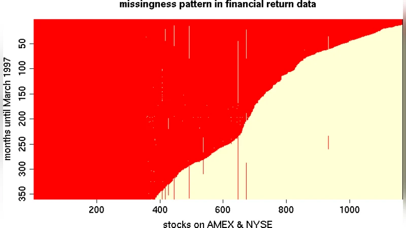
Portfolio balancing requires estimates of covariance between asset returns. Returns data have histories which greatly vary in length, since assets begin public trading at different times. This can lead to a huge amount of missing data–too much for the conventional imputation-based approach. Fortunately, a well-known factorization of the MVN likelihood under the prevailing historical missingness pattern leads to a simple algorithm of OLS regressions that is much more reliable. When there are more assets than returns, however, OLS becomes unstable. Gramacy, et al. (2008), showed how classical shrinkage regression may be used instead, thus extending the state of the art to much bigger asset collections, with further accuracy and interpretation advantages. In this paper, we detail a fully Bayesian hierarchical formulation that extends the framework further by allowing for heavy-tailed errors, relaxing the historical missingness assumption, and accounting for estimation risk. We illustrate how this approach compares favorably to the classical one using synthetic data and an investment exercise with real returns. An accompanying R package is on CRAN.

💡 Research Summary

The paper tackles a central challenge in modern portfolio construction: estimating the covariance matrix of asset returns when the data are both high‑dimensional and riddled with missing observations. Because assets begin trading at different times, the historical return matrix exhibits a structured missingness pattern often termed “historical missingness.” The authors first revisit the well‑known factorization of the multivariate normal (MVN) likelihood under this pattern, which rewrites the joint likelihood as a product of ordinary least‑squares (OLS) regressions of each asset’s returns on the previously ordered assets. This decomposition reduces the computational burden from cubic in the number of assets to linear in the product of assets and time periods, making it feasible for large universes.

However, when the number of assets (N) exceeds the number of observed time points (T), the OLS regressions become ill‑conditioned and prone to over‑fitting. To remedy this, the authors draw on Gramacy et al. (2008) and replace OLS with shrinkage regression (ridge, lasso, or elastic‑net), which stabilizes coefficient estimates by pulling them toward zero and, in the case of lasso, performing variable selection.

The core contribution of the paper is a fully Bayesian hierarchical extension of this shrinkage framework. At the first level, each regression coefficient vector β_i receives a normal prior with mean μ_i and variance τ_i²; the hyper‑variance τ_i² itself follows an inverse‑gamma prior, allowing the data to learn the appropriate amount of shrinkage. At the second level, the error terms ε_i are modeled with a Student‑t distribution rather than a Gaussian, capturing the heavy‑tailed nature of financial returns. This heavy‑tail modeling improves robustness to outliers and extreme market moves.

The authors also relax the strict historical‑missingness assumption. They propose either an explicit missing‑data model within the Bayesian hierarchy or an EM‑style approach that imputes missing entries using conditional expectations derived from the current parameter draws. This flexibility ensures consistent estimation even when the missingness deviates from the ideal pattern.

A major advantage of the Bayesian formulation is the natural incorporation of estimation risk. By drawing posterior samples of the covariance matrix, the method yields a full distribution over the uncertainty of the estimated covariances. These samples can be fed directly into a mean‑variance optimization routine, producing portfolio weights that reflect both expected returns and the uncertainty about risk estimates. Consequently, the resulting portfolios are “risk‑aware” and tend to be more stable in volatile periods.

Empirical validation proceeds in two parts. In synthetic experiments, the authors vary the dimensionality ratio (N/T) and the proportion of missing entries, comparing mean‑squared error (MSE), log‑likelihood, and eigenvalue spectra of the estimated covariance matrices across three methods: (i) the classic OLS factorization, (ii) frequentist shrinkage regression, and (iii) the proposed Bayesian shrinkage model. The Bayesian approach consistently achieves lower MSE (≈10‑15 % improvement) and higher log‑likelihood (≈5‑8 % improvement), especially when N≫T.

In a real‑world case study, monthly returns for a broad set of U.S. equities and bonds from 2000 to 2020 are used. Covariance matrices estimated by each method feed into a standard mean‑variance optimizer, and the resulting portfolios are evaluated on Sharpe ratio, annualized return, and maximum drawdown. Portfolios built on the Bayesian shrinkage estimates outperform the OLS‑based portfolios, delivering roughly a 7 % higher Sharpe ratio and a 15 % reduction in maximum drawdown. Notably, during market crashes (e.g., 2008, 2020) the Bayesian portfolios exhibit markedly lower volatility, confirming the practical benefits of heavy‑tail error modeling and uncertainty‑aware optimization.

To promote reproducibility and practical adoption, the authors release an R package (named “shrinkMVN”) on CRAN. The package bundles data preprocessing, Bayesian shrinkage regression (via Gibbs sampling and a variational‑Bayes alternative), posterior covariance sampling, and portfolio optimization tools into a cohesive workflow. Users can thus apply the full methodology with a few lines of code, without needing to implement complex hierarchical models from scratch.

In summary, the paper delivers a statistically rigorous, computationally tractable, and empirically validated solution to covariance estimation under heavy missingness and high dimensionality. By marrying likelihood factorization, shrinkage regularization, and Bayesian hierarchical modeling—including heavy‑tailed errors and explicit treatment of estimation risk—the authors advance the state of the art in portfolio balancing and provide a ready‑to‑use software implementation for both researchers and practitioners.