A mapping function approach applied to some classes of nonlinear equations

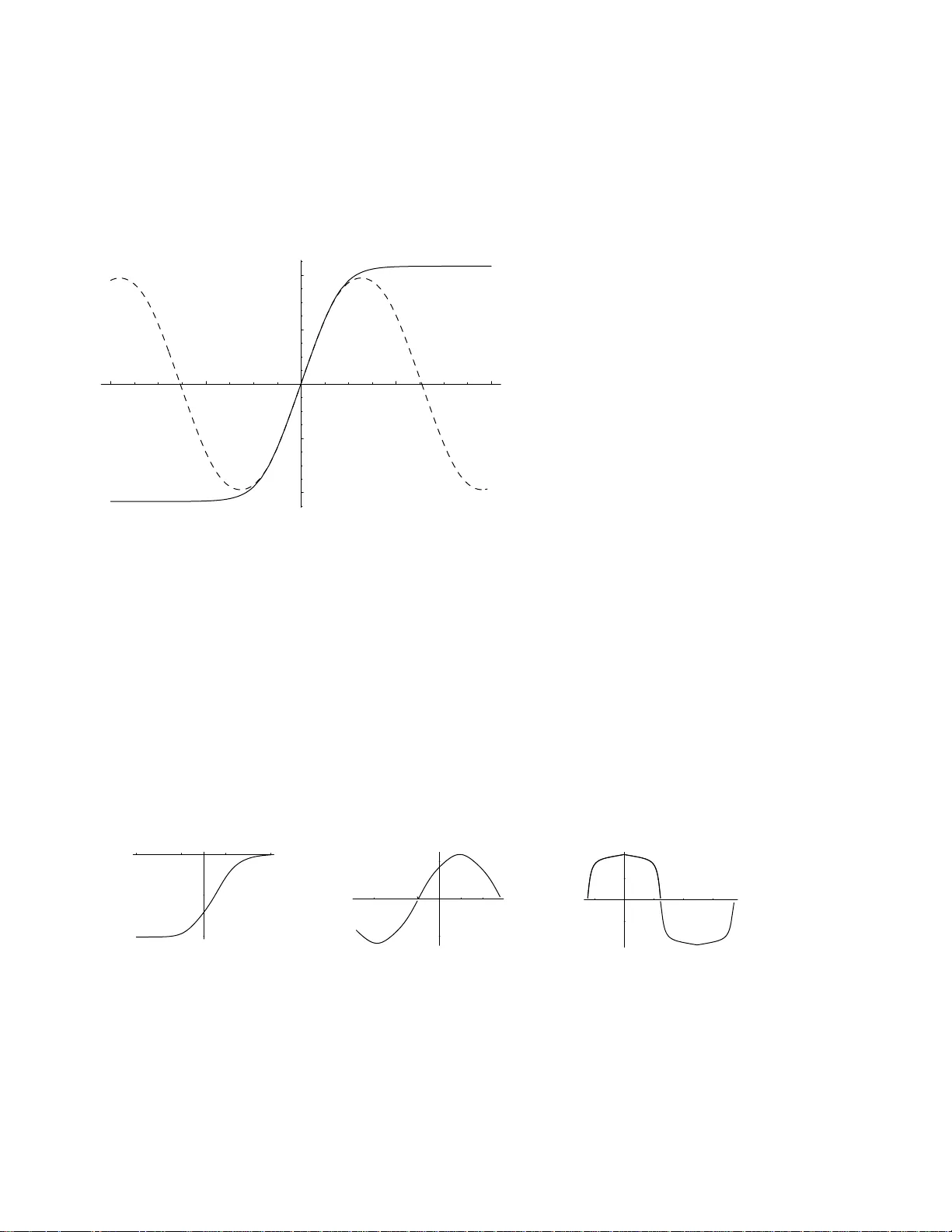
A mapping function approac h applied to some classes of nonlinear equations A. de Souza Dutra a,b ∗ , Marcelo Hott a † and Filip e F. Bellotti a a UNESP Univ Estadual P aulista, Campus de Guaratinguet´ a, Departamen to de F ´ ısica e Qu ´ ımica ‡ 12516-4 10 Guaratinguet´ a, SP , Brasil. b Ab dus Salam ICTP , Strada Costiera 11 , 34014 T rieste Italy . No v em b er 20, 2018 Abstract In this work, we study some mo dels of scalar fields in 1+1 dimensions with non-linear se lf- int eractions. Here, we s ho w ho w it is p ossible to extend the solutions r ecen tly repor ted in the literature for some classe s of nonlinear equations like the nonlinear Klein-Gor don equation, the generalized Camassa- Holm and the Benjamin-Bona-Maho ny equa tions. It is shown t hat the solu- tions obtained by Y omba [1 ], when using the so- called auxiliar y equation metho d, can be r e ac hed by mapping them int o some known nonlinear equations. This is achiev ed through a suitable sequence of translation and p o w er-like trans formations. Particularly , the par en t-like equations used here are the ones for the λφ 4 mo del and the W eier strass equation. This last one, allow us to g et oscillating solutions for the models under ana lysis. W e als o sys tematize the a pproach in order to sho w ho w to get a lar g er class of nonlinear e q uations which, as far as we know, were not taken into account in the literature up to now. P A CS : 02 .30.Jr; 02.30.Gp; 05 .4 5.Yv Key-words: Solitons, Nonlinear equations, Camassa-Holm equation, BBM equation, W eier- strass’ elliptic functions. ∗ Corresponding author: E-mail : d utra@feg. unesp.br Phone:0055-12-312 32848 † E-mail: hott@feg.unesp.br ‡ P ermanent Institution 1 In the last few yea rs, a gro wing n um b er o f w orks hav e b een dev oted to obtain no v el analytical solu- tions for some c lasses of nonlinear differen tial equations, lik e th e n onlinea r Klein-Gordon equation, the generalized C ama ssa-Holm and Benjamin-Bona-Mahon y equations. F or this, man y app r oa c h es w ere dev elop ed. Here we intend to sho w that th r ough a sequen ce of transformations, were one alternates translations and p o w er-lik e transformations, some of the solutions rep orted recen tly in the literature can b e repro duced and, b etter, increased. In particular, w e treat the cases studied by E. Y om ba in a recen t work [1], as well as by J. Nic k el [2]. In those w orks, the auth ors in tro duced interesting metho ds in order to deal essentiall y with an auxiliary equation like  dF ( s ) ds  2 = N X i =0 h i F i . (1) The idea is to sho w that those solutions can b e obtained from a direct mapping with an already kno wn equation lik e, for in stance , the one coming from the so-called λφ 4 mo del. Let us b egin with the Cases 1 and 2 of Y om ba [1]. Starting with the equ at ion  dφ ( s ) ds  2 = A φ 4 + B φ 2 + C , (2) and p erforming the tr ansformation φ =  F − 2 + β  − 1 2 , we arriv e at  dF ( s ) ds  2 = C + ( B + 3 β C ) F 2 +  A + 2 β B + 3 β 2 C  F 4 + β  A + β B + β 2 C  F 6 , (3) whic h is clearly wr itt en in the form app earing in the w ork [1], namely  dF ( s ) ds  2 = h 0 + h 2 F 2 + h 4 F 4 + h 6 F 6 . (4) A t this p oin t w e should obser ve th at , in order to mak e con tact with the solution app earing in [1 ], w e must fix the arb itrary parameter β suc h th at β = 3 h 4 8 h 2 . Once this p articular c hoice is m ade, the restrictions app earing in th e Case 1 of [1] ( h 0 = 8 h 2 2 27 h 4 , h 6 = h 2 4 4 h 2 ) are reco v ered. S o, one can conclude that the fr ee dom introduced by means of the arb itrary p aramet er β , allo ws us to get less restrictiv e solutions. In f act, as we are go ing to see b elo w, th is mapping allo ws to get, b esides the trigonometric and h yp erb olic solutions, some other oscil lating ones coming f rom the solutions o f the W eierstrass equation [3], [4]. F urthermore, as it can b e s ee n, if one c ho oses the particular case where C = 0 (Case 2) in the equation (2), one obtains th e relations, 2 B = h 2 , A = ǫ √ ∆ , β = h 4 + ǫ √ ∆ 2 h 2 , (5) where ǫ = ± 1 and ∆ = h 2 4 − 4 h 2 h 6 , as defined in the T able 2 of [1]. Note that, due to the restricted c h oice of the parameter C ( C = 0), the solutions of equation (2) sh al l b e give n b y φ ( s ) = 2 h 2 e ± √ h 2 s 1 − ǫ h 2 ∆ e ± 2 √ h 2 s , (6) and the solutio n for the fun ctio n F ( s ) is simply obtained b y dir ec t substitution in the equation F (2) = ±  φ 2 − β  − 1 / 2 . Before g oing further in our analysis, w e should mention that the Case 5 of [1] can b e obtained from this last case treated ab o v e, by m aking th e additional trans formatio n F (2) = ± F 1 / 2 (5) . Then, we obtain the follo win g equation  dF (5) ( s ) ds  2 = h 2(5) F 2 (5) + h 3(5) F 3 (5) + h 4(5) F 4 (5) , (7) where one sh all mak e the identificat ions: h 2(5) = 4 h 2(2) , h 3(5) = 4 h 4(2) and h 4(5) = 4 h 6(2) . Thus, w e see that the discriminant defined for this case comes f r om the one of the Case 2 and is giv en by ∆ (5) = h 2 3(5) − 4 h 2(5) h 4(5) = 16 ∆ (2) . The notation h i ( j ) stands for the i-th co efficien t of the j-th case. No w, w e defin e “generations” of equations whic h can b e obtained from the important non lin ea r W eierstrass differentia l equation  d℘ ds  2 = 4 ℘ 3 − g 2 ℘ − g 3 , (8) whic h, as it is kn o wn, can p resen t solutions in many regimes, according to the sp ecific c h oice of the invariants g 2 and g 3 and of the discriminant ∆ = g 2 3 − 27 g 3 2 . Those solutions include, trigonometric and hyper b olic solutions as well as other oscillating solutions in terms of th e Jacobi elliptic functions. What we call the “zero-th” g eneration is trivially o btained from the W eierstrass equation by simply p erforming a translation and a dilation lik e F 0 ( s ) = a ℘ ( s ) + b . In this generation, one h as a quadratic term in the differen tial equation. One can c hec k that the Case 4 of [1] is completely r eco v ered, including the same constraints relating the co effici en ts of the p olynomial on th e right hand s id e of the equation. The next generation is obtained by doing the transformation ℘ ( s ) = r ( F I ) α ( r and α are arbitrary constan ts) a nd, if one is in terested only in p olynomials with p ositiv e and integ er degrees in F I , one m ust c h oose α = − 1 or α = − 2. In su ch cases, one obtains: 3  dF I a ( s ) ds  2 = 4 r F I a − g 2 r F 3 I a − g 3 r 2 F 4 I a , for α = − 1 , (9) and  dF I b ( s ) ds  2 = r − g 2 4 r F 4 I b − g 3 4 r 2 F 6 I b , for α = − 2 . (10) The second generation comes from a translation p erf orm ed on the fun ctio ns of the first generation. F or instance, by d oi ng the transform at ion F I a ( s ) = F I I a ( s ) + k one is left with  dF I I a ( s ) ds  2 = h 0 + h 1 F I I a + h 2 F 2 I I a + h 3 F 3 I I a + h 4 F 4 I I a , (11) where h 0 = − k r 2  g 3 k 3 + g 2 r k 2 − 4 r 3  , h 1 = 1 k r 2  4 r 3 − 4 k 3 g 3 − 3 r k 2 g 2  , h 2 = − 1 r 2 [3 k (2 k g 3 + r g 2 )] , h 3 = − 1 r 2 (4 k g 3 + r g 2 ) and h 4 = − g 3 r 2 . It is evid ent th at we ha v e no longer the co efficien ts indep endent of eac h other. At this p oin t we can mak e the identi fications defin ed in [1], α = h 4 , β = h 3 4 , γ = h 2 6 , ǫ = h 0 , and v erify that the constraints app earing in th e Case 3 of [1] and also in [2], namely g 2 = α ǫ − 4 β δ + 3 γ 2 and g 3 = α γ ǫ + 2 β γ δ − α δ 2 − γ 3 − ǫ β 2 are repro duced and, as a consequence, th e discriminant of the system will b e necessarily the same one for the W eierstrass equation: ∆ = g 3 2 − 27 g 2 3 . In this case the solution of the functions F I I a are written in terms of the W eierstrass fun cti on as F I I a ( s ) = r ℘ − 1 ( s ) − k . Finally , th e Case 6 of [1] is precisely the equation (2), which we ha v e commenced the m apping of the first t w o cases of [1]. No w, w e sho w that, for the cases wh er e the three constants A, B , C are arbitrary , equation (2) can b e mapp ed into th e W eierstrass equation. F or this w e can set φ ( s ) = √ C  ℘ ( s ) − B 3  − 1 2 or φ ( s ) = 1 √ A  ℘ ( s ) − B 3  1 2 , leading us to the equation (8 ) with g 2 = 4 C  B 2 3 C − A  and g 3 = 4 C B  A 3 − 2 B 2 27 C  . (12) for the fir st case or 4 g 2 = 4 A  B 2 3 A − C  and g 3 = 4 A B  C 3 − 2 B 2 27 A  . (13) in the second ca se. In fact, if one is inte rested in non-singular solutions, one must c ho ose the first solution, since the W eierstrass fun ction alw ays present s singular p oints whic h, in that case, will lead to we ll-b eha ve d solutions. In the Figure 1, some examples of those con tinuous solutions are p resen ted. Since w e ha v e sho wn ho w to obtain all the cases studied in [1] b y means of a mapping appr oa c h, w e can g o further with th e pro ce dure b y getting no vel equations whose solution can b e reac hed b y using this metho d. In fact, we can obtain terms of higher degrees p olynomial on the right hand side of the auxiliary d iffe rent ial through a suitable com b inati on of p o wer-lik e and translation transformations on the W eierstrass different ial equation. Ho w ev er, in order to achiev e this goal, one must c h o ose the translation constant appr opriate ly . F or example, let u s start w ith the W eierstrass equation and mak e the transformation ℘ ( s ) = ( k + F ( s ) 2 ) − 2 , w hic h leads u s to the equation  dF ( s ) ds  2 = a 0 + a 2 F 2 + a 4 F 4 + a 6 F 6 + a 8 F 8 + a 10 F 10 , (14) where w e h a v e fixed the inv ariant g 3 as g 3 = 4 − g 2 k 4 k 6 in ord er to a v oid a term with negativ e p o w er on the righ t hand sid e of the differentia l equ at ion. Un der this condition, the co efficie n ts a i are given by a 0 = ( − 12 + g 2 k 4 ) / (8 k ) , a 2 = 3( − 20 + 3 g 2 k 4 ) / 16 k 2 , a 4 = ( − 5 + g 2 k 4 ) /k 3 , a 6 = ( − 30 + 7 g 2 k 4 ) / 8 k 4 , a 8 = 3( − 4 + g 2 k 4 ) / 8 k 5 , a 10 = ( − 4 + g 2 k 4 ) / 16 k 6 . (15) Note th at , ev en if we includ e an additional parameter th rough a scaling of the fu nction, we still ha v e only three free p aramete rs, the remaining ones sh ould b e fi xed in order to gran t the exact solv abilit y of th e equation. Some solutions for th is example are illustr at ed in the Figure 2. One can see that the approac h develo p ed h ere generates higher order exactly solv able differen tial equations. W e think that those can b e u s eful to a b etter understand in g of some classes of nonlin ear equations lik e the generalize d Camassa-Holm and the Benjamin-Bona-Ma hon y equations, as d on e b y Y om ba [1] and the n onlinear Klein-Gordon equation and their generalizatio ns as the sine-Gordon, the sinh-Gordon and their m odified ve rsions, as considered b y [5]. In ord er to illustrate the mapp ing app roac h ev en more, we would lik e to consider h ere n on-linea r mo dels in volving th e Jacobi elliptic functions, particularly wh at has b een called th e Jacobi mo del [6], 5 whose auxiliary differentia l equ at ion is  dφ ds  2 = 4 sn 2 ( φ 2 | m ) − 4 c 2 , (16) where c is a constan t of the integ ration and s n ( ϕ | m ) is th e Jacobi elliptic fu nction defin ed by sn ( ϕ, m ) = sin θ , with resp ect to the integ ral ϕ = θ R 0 dα/ (1 − m sin 2 α ) 1 / 2 , where θ is called the amplitude and m (0 ≤ m ≤ 1) is the el liptic p ar ameter . The equation (16) retrieve s th e one f or the s o-called sine-Gordon mo del for m = 0. W e h a v e noted, b y using the mapping approac h, that the ab o v e equation has oscillat ing solutions for 0 < c 2 < 1 and soliton solutions for c 2 = 0. T he redefinition of the fields F ( s ) = cn ( ϕ ( s ) | m ), w h ere cn ( ϕ | m ) is the J ac obi elliptic function defined b y cn ( ϕ | m ) = cos θ , maps th e equation (1 6) in to an equat ion iden tical to (1) with N = 6 and the co effici en ts give n by h 0 = 1 − m − c 2 + c 2 m, h 2 = − 2 + c 2 + 3 m − 2 c 2 m, h 4 = 1 − 3 m + c 2 m, h 6 = m. (17) By using the follo wing m apping F = ± p h 0 ( ℘ + κ ) − 1 / 2 (18) with κ = 1 / 3(2 − c 2 − 3 m + 2 c 2 m ), w e r ec o ver the W eierstrass d ifferen tial equation (8) satisfied by the W eierstrass elliptic f unction ℘ ( s ; g 2 , g 3 ) with the inv ariant s g 2 = 4 / 3(1 − c 2 (1 + m ) + c 4 (1 − m + m 2 )) , g 3 = − 4 / 27(2 − 3 c 2 (1 + m ) − 3 c 4 (1 − 4 m + m 2 ) + c 6 (2 − 3 m − 3 m 2 + 2 m 3 ) . (19) A t this p oin t we can use th e r ela tion 18.9.1 1 of the reference [4], whic h relates the W eierstrass and the Jacobi elliptic functions, since th e discrimin an t ∆ > 0. Then w e obtain ℘ ( s ) = e 3 + ( e 1 − e 3 ) /sn 2 (( e 1 − e 3 ) 1 / 2 s | ν ) , (20) where e 1 = 1 / 3(1 + c 2 − 2 c 2 m ) , e 2 = 1 / 3(1 − 2 c 2 + c 2 m ) , e 3 = 1 / 3( − 2 + c 2 + c 2 m ) (21) and ν = ( e 2 − e 3 ) / ( e 1 − e 3 ) = (1 − c 2 )(1 − c 2 m ) . (22) Finally the solution f or the Jacobi elliptic mo del can b e written as φ J a cobi ( s ) = 2 cn − 1 ( F ( s ) | m ) , (23) 6 with F ( s ) = ± p (1 − c 2 )(1 − m ) sn ((1 − c 2 m ) s | ν ) p (1 − c 2 m ) − (1 − c 2 ) m sn 2 ((1 − c 2 m ) s | ν ) . (24) The ab o v e expression is the solution for the equation (1) with N = 6 and co effici en ts h i giv en in (17). According to the classification sc h eme mentioned ab o v e, it b elongs to the 2nd generation ( F I I b ). By ta king c = 0 in equations (22 )-( 24) w e obtain the (anti-)kink soliton solutions for t he J ac obi elliptic mo del φ J a cobi ( s ) = 2 cn − 1   ± p (1 − m ) tanh s p 1 − m tanh 2 s       m   (25) The k ink solution ab o v e can b e r ewritte n as φ k ink − J acobi ( s ) = 2 K [ m ] + 2 sn − 1 (tanh s | m ), which is the kink foun d in [6], and K [ m ] is the elliptic qu arte r p erio d. The solutions for the sin e- Gordon model are retriev ed b y taking m = 0. In this limit the differen tial equation for F ( s ) is the equation (1) with N = 4; th e coefficien ts can b e obtained fr om (17) by taking m = 0. The solution for th e sine-Gordon mo del is φ s − G ( s ) = 2 cos − 1 ( ± p 1 − c 2 sn ( s | 1 − c 2 )) , (26) whic h is in agreemen t with the solution presented in [7] and [8] with an adequate reparametrization of the v ariable s and a reescaling of the field. F or c = 0 w e o btain the (anti-)kink solution for t he sine-Gordon mo del φ s − G ( s ) = 2 cos − 1 ( ± tanh s ) = 4 tan − 1 ( e ∓ s ) . (27) Finally w e w ould like to ment ion that generalizations of non-p olynomial non-linear mo d els as for instance, the generalized versions of the sine-Gordon and the sin h -Go rdon mo dels [5], can also b e approac h ed by means of this mapping fun ct ion metho d describ ed here. Ac knowledgmen ts: The authors thanks to CNPq and F APESP for partial fi nancial supp ort. This w ork wa s partially d one during a visit (A.S.D.) with in the Asso cia te S c heme of the Ab du s S al am ICTP . References [1] E. Y om ba, Ph ys. Lett. A 372 (2008) 1048-1060 , and references th erein. [2] J. Nic ke l, Ph ys. Lett. A 364 (2007) 221-226, and references therein. 7 [3] E. T. Whittak er and G.N. W atson, A Course of Modern Analysis, Cambridge Univ ersit y Press, London, 1927. [4] M. Abramo witz and I. Stegun, Handb o ok of Mathematical F unctions, Do v er, T oron to, 1965. [5] A-M. W azwaz , Chaos, Solitons and F ractals 28 (2006) 127-135 [6] G. V. Dunne, Ph ys. Lett. B 467 (1999) 238-2 46. G.V. Dunne and K . Rao, JHEP 01 (2 000) 019-02 5. [7] K. T ak a ya ma and M. Ok a, Nucl. Phys. A 551 (1993) 637-6 56. [8] G. Mussardo, V. Riv a and G. Sotko v, Nu cl. Ph y s . B 705 [FS] (2005) 548- 562. 8 -4 -2 2 4 x -0.4 -0.2 0.2 0.4 Φ H x L Figure 1: Solutions of the equation (2) with ∆ = 0, g 2 = 12 and g 3 = − 8 (solid line) and ∆ > 0, g 2 = 13 and g 3 = − 8 (d ashed line) -3 -1 1 3 x -0.7 -1.4 F H x L -3 -1 1 2 x -1 1 F H x L -1 1 2 3 x -1 1 F H x L Figure 2: Solutions of th e equation (14) for ∆ = 0, g 2 = 12 and g 3 = − 8 (left fi gure); ∆ > 0, g 2 = 20 and g 3 = − 8 (mid dle figure) and ∆ < 0, g 2 = − 20 and g 3 = 1 (righ t figure) 9