Markov basis and Groebner basis of Segre-Veronese configuration for testing independence in group-wise selections

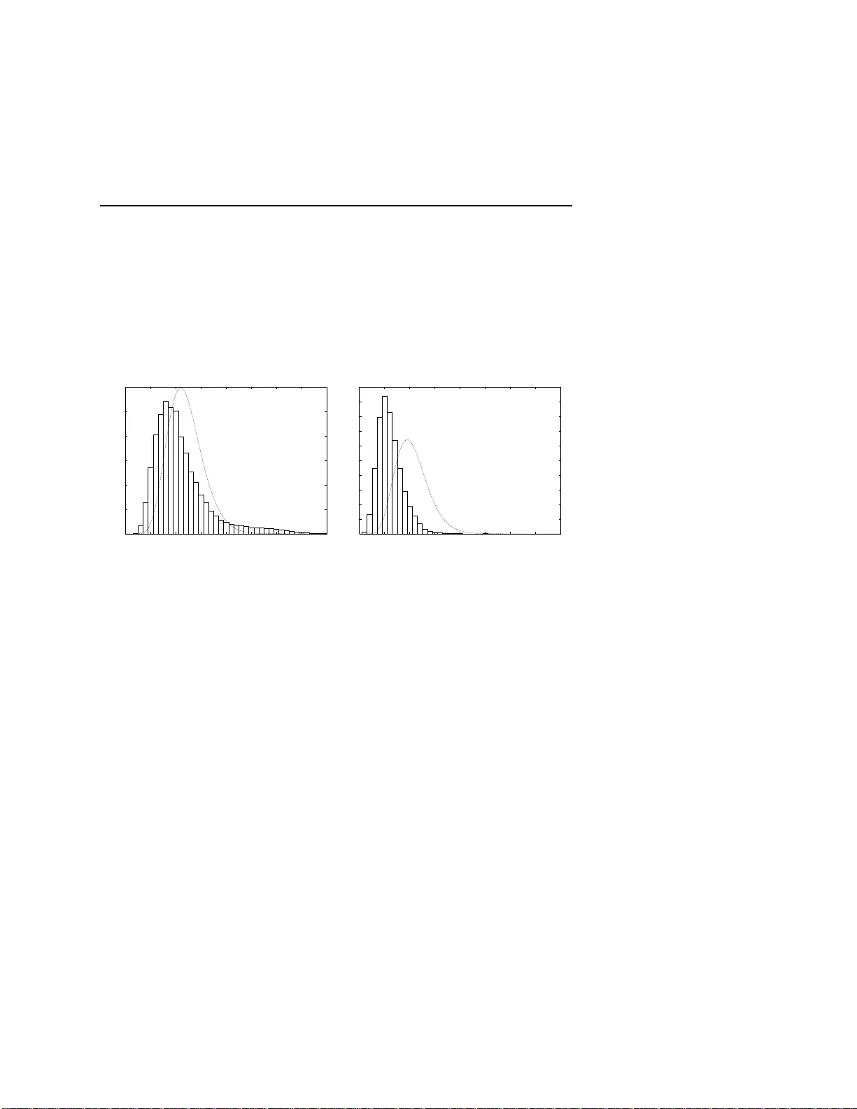
Annals of the Institute of Stat istical Mathematics man uscript No. (will be inserted by the editor) Mark o v basis and Gr¨ obner basi s of Segre-V eronese configuration for testing indep endence in gr o up-wise selections Satoshi Aoki · T ak a yuki Hi bi · Hidefumi Ohsugi · Akimic hi T ak emura Receiv ed: dat e / Revised: date Abstract W e co nsider testing independence in gr oup-wise selections with some restrictions on com binations of choices. W e present models for frequency data of selectio ns for which it is easy to p e rform conditional tests by Marko v chain Monte Carlo (MCMC) methods. When the restrictions on the combina- tions can b e describ ed in terms of a Segr e-V erones e configuratio n, a n ex plicit form o f a Gr¨ obner basis cons isting of binomials o f degree tw o is readily av ail- able for perfor ming a Marko v c hain. W e illustrate our setting with the National Cent er T est for university en trance exa minations in J apan. W e a lso a pply our metho d to testing indepe ndence hypotheses involving genotypes at more than one lo cus or haplotype s of a lleles on the same chromosome. Keyw ords contingency table · diplotype · exact tests · ha plot yp e · Hardy- W einberg mo del · Marko v c hain Mont e Carlo · Nationa l Center T e st · structural zero Satoshi Aoki Departmen t of Mathematics and Computer Science Kagoshima Universit y 1-21-35, Korimoto, Kagoshima, Kagoshima 890-0065, Japan E-mail: aoki@sci.k agoshima-u.ac.jp T ak ayuki Hibi Graduate Sc ho ol of Information Science and T echnology Osak a Universit y 1-1, Y amadaok a, Suita, Osak a 565-0871, Japan Hidefumi Ohsugi Departmen t of Mathematics Rikkyo Universit y 3-34-1, Nishi Ik ebukuro, T oshima-ku, T okyo 171-8501, Japan Akimichi T ak emura Graduate Sc ho ol of Information Science and T echnology Unive rsity of T oky o 7-3-1, Hongo, Bunky o-ku, T oky o 113-0033, Japan 2 Satoshi Aoki et al. 1 Introduction Suppo se that pe ople are asked to select items which a re classified into cate- gories o r groups and there ar e some restr ictions on combinations of choices. F o r example, when a consumer buys a car, he o r she ca n cho ose v ar ious o ptions, such as a co lor, a g rade of air conditioning , a br a nd of audio eq uipmen t, etc. Due to space res trictions for exa mple, some c o m bina tions of o ptions may not be av ailable. The problem we consider in this pap er is testing indep endence o f peo ple’s pr e ferences in group-wise selections in the presence o f restr ictions. W e assume that obser v ations are the counts of p eople choo sing v ar ious combina- tions in g roup-wise selections, i.e., the data ar e given in a form of a multiw ay contingency table with some s tr uctural zero s co rresp onding to the restr ic tions. If there are m gro ups of items and a co nsumer freely cho oses just one item from each g roup, then the combination o f choices is simply a ce ll of an m - wa y contingency table. Then the hypo thesis o f independence reduces to the complete indep endence model of an m -wa y c ont ing ency ta ble . The pro ble m bec omes harder if there are s ome a dditional conditions in a group-wise se- lection. A consumer ma y b e asked to choo se up to tw o items from a group or there may be a r estriction on the to tal num b er of items. Groups may be nested, so that there are further res trictions on the num b er of items fro m sub- groups. Some r estrictions may concern several groups or subgr oups. Therefore the restrictions on combinations may be complicated. As a concr ete example we consider r estrictions on choo s ing sub jects in the National Center T est (NCT her eafter) for university entrance examinations in J apan. Due to time constraints of the schedule of the test, the pattern of restrictions is rather complicated. Howev er we will show that restrictio ns o f NCT can b e descr ibed in terms o f a Segre-V eronese configur a tion. Another imp ortant applicatio n of this pap er is a generalizatio n o f the Hardy-W einber g mo del in p opulatio n ge netics. W e are interested in testing v arious hypotheses of indepe ndence inv olving genotypes at mo r e than one lo cus and haplo t yp es of c o m bina tion of alleles on the sa me chromosome. Although this problem seems to b e different fr o m the ab ov e intro ductory motiv ation on consumer c hoices, we c an imag ine that each offspring is r equired to cho ose tw o alleles for e ach gene (lo cus) from a p o ol of alleles for the gene. He or she can choose the same allele twice (ho mo zygote) o r different a lleles (hetero z y gote). In the Ha rdy-W einberg mo del tw o choices a re ass umed to b e indep endent ly and identically distributed. A natural g eneralization of the Hardy-W ein b erg mo del for a single lo cus is to consider indepe ndence of g enotypes o f more than one lo cus. In many epidemiologica l studies, the primary interest is the cor- relation b etw een a cer tain disea se and the genotype of a s ing le g ene (or the genotypes at more than one lo cus, or the haplotypes involving alleles on the same chromosome). F urther complication might a rise if certain ho mo zygotes are fatal a nd can not b e observed, thus b ecoming a s tr uctural zer o. In this pap er we c o nsider c o nditional tests o f indep endence hypotheses in the ab ov e t wo imp ortant problems from the vie wpoint of Marko v bases and Gr¨ obner bases. Ev aluation of P -v alues by Ma rko v chain Mo n te Ca rlo (MCMC) Gr¨ obner basis for testing independence in group-wise selections 3 metho d using Mar ko v base s and Gr¨ obner bas es was initiated in Diaconis and Sturmfels (1998 ). See also Sturmfels (1995). Since then, this approach at- tracted m uch atten tio n from statisticians as well as a lgebraists. Contributions of the present author s ar e found, for e x ample, in Aok i and T akem ura (200 5, 2007), Ohsugi and Hibi (200 5, 20 06, 20 07), and T ak emura a nd Aoki (20 04). Metho ds of alg e braic sta tis tics are curr en tly ac tiv ely a pplied to proble ms in computational biology (Pach ter and Sturmfels, 200 5). In a lgebraic statistics, results in co mmutative alge br a may find somewhat unexp ected applica tio ns in statistics. At the sa me time statistica l pro blems may prese n t new problems to commutativ e algebr a. A rece nt example is a c o njunctiv e Bay esia n netw ork prop osed in Beerenwinkel et al. (20 06), where a result of Hibi (1987 ) is succes s- fully used. In this pap er we present application of results on Segr e-V erones e configuratio n to testing indep endence in NCT and Hardy-W einberg mo dels. In fact, these statis tica l consider ations hav e prompted further theore tica l devel- opments of Gr¨ obner ba ses for Seg r e-V ero nese type configura tions and we will present these theoretical results in our subsequent pap er (Aoki et al., 2 007). Even in tw o -wa y tables, if the po sitions of the structur a l zero s are arbitra ry , then Markov bases may contain mov es of hig h deg rees (Aoki and T a kem ura, 2005). See also Huber et al. (2006) and Rapallo (20 06) for Marko v bases of the problems with the str uctural zer os. How ever if the restrictio ns on the combinations can b e describ ed in terms o f a Segr e-V ero ne s e configuration, then an explic it fo rm of a Gr¨ obner basis consisting of binomials of degree t wo with a squar efree initial term is readily av a ilable for running a Mar ko v chain for p erforming co nditional tests of v arious hypothes e s of indep endence. Therefore mo dels which ca n be describ ed by a Seg re-V ero nese config uration are very us e ful for statistica l analys is. The organization of this pap er is as follows. In Section 2 , we in tro duce t wo examples of group- wise se le ction. In Section 3, we give a for malization of conditional tests and MCMC pr o cedures and co ns ider v arious hyp o theses of independence for NCT data and the allele freq uency data. In Section 4, we define Segre-V eronese configura tion. W e giv e an ex plicit expressio n o f a reduced Gr¨ obner basis for the configur ation and describ e a simple pro cedure for running MCMC using the basis for co nditio na l tests. In Se c tion 5 we present nu merical r esults on NCT data a nd diplotype frequencies data. W e end the pap er by some discussio ns in Section 6. 2 Exampl e s of group-wis e s elections In this sectio n, we int ro duce tw o examples of group-wis e selection. In Section 2.1, w e take a close lo o k at patterns of selections of sub jects in NCT. In Section 2 .2, we illus trate an imp orta n t problem of p opulation genetics from the viewp oint of gr oup-wise selectio n. 4 Satoshi Aoki et al. 2.1 The ca s e of Nationa l Center T es t in Japa n One impor tan t exa mple of group-w is e se le ction is the entrance examination for universities in J a pan. In Japa n, a s the co mmo n fir s t-stage screening pro - cess, most studen ts apply ing for universities take the Na tio nal Center T est for universit y en trance examinations administered by Nationa l Cen ter for Univer- sity E n tr ance E xaminations (NCUEE). Basic info r mation in English on NCT in 200 6 is av ailable from the b o oklet published by NCUEE ([12 ] in the refer- ences). After obtaining the score of NCT, students apply to depa rtmen ts of individual universities and take second-stage examina tions administered by the universities. Due to time c o nstraints of the schedule of NCT, ther e are ra ther complicated r estrictions on po ssible combination of sub jects. F urthermore each department o f each university can imp ose different a dditio nal requirement on the combinations of sub jects of NCT to students applying to the department. In NCT examinees c an choo se sub jects in Mathematics, So cial Studies and Science. These three ma jor sub jects are divided into sub categor ies. F or example Ma thematics is divided into Mathematics 1 and Ma thematics 2 a nd these are then co mp osed of indiv idua l sub jects. In the test carried out in 2006 , examinees could se lect tw o mathema tics sub jects, tw o so cial studies sub jects and three science s ub jects at most as shown b elow. The details of the sub jects can be found in w eb pages and publications of NCUEE. In this pape r , w e omit Mathematics for simplicit y , and only consider selections in Socia l Studies and Science . In parentheses w e show our a bbreviations for the s ub jects in this pap er. – So cial Studies: ◦ Geogra phy and History: One sub ject from { W o rld Histor y A (WHA), W orld History B (WHB), J apanese History A (JHA), Japanese History B (JHB), Geogra ph y A (GeoA), Geog raphy B (GeoB) } ◦ Civics: One sub ject fr om { Contemporary Socie ty (Con tSo c), Ethics, Politics and E conomics (P& E) } – Science: ◦ Science 1: One sub ject from { Co mpr ehensive Scie nce B (CSciB), Biol- ogy I (Bio I ), Integrated Science (IntegS), Biology IA (BioIA) } ◦ Science 2: One sub ject from { Comprehensive Science A (CSciA), Chem- istry I (ChemI), Che mis try IA (ChemIA) } ◦ Science 3: One sub ject fro m { Physics I (Ph ysI), Ea rth Science I (EarthI), Physics IA (P hysIA), Earth Science IA (E arthIA) } F requencies of the examinees selecting each combination of sub jects in 2006 are given in the website o f NCUEE. W e r epro duce part of them in T a bles 8– 12 at the end of the pap er. As seen in these tables, examinees may select or not select these sub jects. F or example, o ne ex aminee may select tw o sub jects from So cia l Studies and three sub jects fro m Science, while another exa minee may select o nly one sub ject from Scie nc e and none from So cial Studies. Hence each exa minee is catego rized in to o ne of the (6 + 1) × · · · × (4 + 1) = 2 800 combinations o f individual sub jects. Here 1 is added for not c ho osing from Gr¨ obner basis for testing independence in group-wise selections 5 the sub categ ory . As mentioned ab ov e, individual depar tmen ts of universities impo se different additional r equirements on the choices of sub jects of NCT. F or example, many science or engineering departments of national universities ask the students to take tw o sub jects from Science and o ne sub ject fro m So cial Studies. Let us obser ve some tendencies of the s elections by the exa minees to illus - trate wha t kind o f sta tis tica l q uestions o ne might ask concerning the data in T ables 8 – 1 2. (i) The most freq uen t triple of Science sub jects is { Bio I, ChemI, Ph ysI } in T a- ble 12, w hich seems to b e co nsistent with T able 10 since these three sub jects are the mo st fre q uen tly selected sub jects in Science 1, Science 2 and Sci- ence 3, res pectively . How ever in T able 11, while the pairs { BioI, ChemI } and { Che mI, P h y sI } are the most frequently sele c ted pair s in { Science 1 , Science2 } and { Science 2 , Science 3 } , resp ectively , the pair { BioI, PhysI } is not the first ch oice in { Science 1, Science 3 } . This fact indicates differences in the selection of Science sub jects betw e en the e x aminees selecting tw o sub jects and those selecting three sub jects. (ii) In T able 9 the most freque nt pa ir is { GeoB , ContSoc } . How ever the most frequent single sub ject from Geogr aphy and Histor y is JHB b oth in T able 8 a nd 9. This fact indicates the in ter action effect in selecting pa irs of So cial Studies. These o bserv ations lea d to many interesting statistical questions . How ever T ables 8 – 12 only give frequencie s o f choices separ ately for So cial Studies a nd Science, i.e., they are the marginal tables for these tw o ma jor sub jects. In this pap er we ar e interested in independenc e a cross these tw o sub jects, such as “ar e the selections on So cia l Studies a nd Science related or not?” W e give v arious mo dels for NCT data in Sec tion 3.2 and numerical ana ly sis in Sectio n 5.1. 2.2 The ca s e of Har dy -W einberg mo dels for allele fr e quency data W e also consider pr oblems of p opulation g enetics in this paper . This is another impo rtant application o f the metho dolog y of this pap er. The allele fr e quency data are usua lly given a s the genotype fre q uency . F or multi-allele lo cus with alleles A 1 , A 2 , . . . , A m , the pr obability of the g enotype A i A j in a n individual from a ra ndo m br eeding p opulation is q 2 i ( i = j ) or 2 q i q j ( i 6 = j ), where q i is the prop ortion o f the allele A i . These are known as the Hardy- W ein b erg equi- librium pro ba bilities. Since the Hardy-W ein b erg law plays an imp ortant r ole in the field of p opulation genetics and often ser ves a s a basis for genetic infer- ence, muc h attention ha s b een pa id to tests of the h yp othesis that a p opulatio n being sa mpled is in the Hardy-W e inber g equilibrium ag ainst the hypothesis that disturbing fo r ces cause some deviation fro m the Hardy-W ein b erg ratio. See Cr ow (198 8) and Guo and Thompson (1992) for example. Though Guo and Thompso n (1992) consider the exact test of the Hardy W einberg equi- librium for mu ltiple lo ci, exact pro cedure be c omes infeasible if the data size 6 Satoshi Aoki et al. or the n umber of alleles is mo derately large. Therefor e MCMC is a lso use- ful for this problem. T a k emura and Ao ki (200 4) considers conditional tests o f Hardy-W einber g mo del by using MCMC a nd the technique of Ma r ko v bases. Due to the rapid pro g ress of se q uencing technology , more and mo r e infor- mation is av ailable on the combination of a lle les on the same chromosome. A combination of alleles a t more than o ne lo cus on the same chromosome is called a haplotype and data on haplotype counts are called haplotype frequency data . The haplo type analy sis has gained an increasing attention in the mapping of complex-diseas e genes, because of the limited pow er of conven tional single - lo cus analyses. Haplotype data may come with or without pairing informatio n on ho mologous chromosomes. It is techn ically more difficult to determine pairs of haplotypes of the co rresp onding lo ci on a pa ir of homolo gous chromosomes. A pa ir of haplot yp es on homologous chromoso mes is called a diplotype. In this pap er we a r e interested in diplotype fre q uency data, b ecause ha plot yp e frequency data o n individua l chromosomes without pairing information a re standard contingency table da ta and can b e a na lyzed by statistical metho ds for usual contingency tables. F or the diplotype frequency data , the null mo del we wan t to consider is the indep endence mo del that the pr o bability for each diplotype is expressed by the pro duct of pr obabilities fo r ea c h geno t yp e. W e consider the mo dels for ge no t y p e frequenc y data in Sectio n 3.3.1 a nd then consider the mo dels for diplotype frequency data in Section 3.3.2 . Note that the av aila bilit y of haplotype data or diplotype data requir es a separ ate treatment in our arg umen ts. Finally we give numerical examples of the a nalysis of diplotype fr equencies da ta in Section 5.2. 3 Condi tional tests and mo dels 3.1 General formulation o f co nditional tests and Mar ko v chain Monte Ca rlo pro cedures First we give a br ief r eview on p e rforming MCMC for conducting conditiona l tests based on the theo ry of Ma rko v basis. Markov basis was intro duced by Diaconis and Sturmfels (1998) a nd ther e are now many refere nc e s o n the def- inition and the use of Mar ko v bas is (e.g. Aoki and T ak emura, 200 6). W e denote the s pa ce of po ssible selections as I . Ea ch element i in I rep- resents a combination o f c hoices. F ollowing the termino logy o f con tingency tables, each i ∈ I is ca lled a c el l . It should b e noted that unlik e the case o f standard multiw ay contingency tables, our index set I can not b e written as a direct pro duct in gener al. W e show the structur e s o f I for NCT da ta a nd allele fr equency data in Section 3 .2 a nd Section 3.3 , resp ectively . Let p ( i ) denote the proba bilit y of selecting the combination i (or the pr ob- ability of cell i ) a nd write p = { p ( i ) } i ∈I . In this pap er, we do not necess a rily assume that p is no rmalized. In fact, in the mo dels we consider in this pa- per , we only g ive an unnor malized functional sp ecification o f p ( · ). No te that we need not calculate the normalizing constant P i ∈I p ( i ) for performing a Gr¨ obner basis for testing independence in group-wise selections 7 MCMC pro cedure. Denote the result o f the selections by n individua ls as x = { x ( i ) } i ∈I , where x ( i ) is the freq uenc y of the cell i . W e ca ll x a freq uenc y vector. In the models considered in this pap er, the cell proba bilit y p ( i ) is written as some pro duct of functions, which cor r esp ond to v ario us marginal pro babilities. Let J deno te the index se t of the mar ginals. Then our mo dels ca n be written as p ( i ) = h ( i ) Y j ∈J q ( j ) a ji , (1) where h ( i ) is a known function a nd q ( j )’s are the para meters. An imp orta n t po in t here is that the s ufficie nt statistic t = { t ( j ) , j ∈ J } is wr itten in a matrix form a s t = A x , A = ( a ji ) j ∈J , i ∈I , (2) where A is d × ν matrix of non-negative in teg e rs and d = |J | , ν = |I | . W e call A a c onfigu r ation in connection w ith the theo ry of toric ideals in Section 4 . By the s tandard theory of conditional tests (Lehmann a nd Romano, 2005 , for example), w e can p erform conditiona l test of the mo de l (1) based on the conditional distribution given the sufficient statistic t . The conditional sample space given t , called the t - fiber , is F t = { x ∈ N ν | t = A x } , where N = { 0 , 1 , . . . } . If we can sample from the conditional distribution ov er F t , we can ev alua te P -v alues of any test s tatistic. One o f the adv antages of MCMC method of sampling is that it can b e run without ev aluating the normalizing co nstant. Also once a connected Mar ko v chain ov er the conditional sample spa ce is constructed, then the chain can be mo dified to give a connected and ap erio dic Markov chain with the stationar y distr ibution b y the Metrop olis- Hastings pro cedur e (e.g. Hastings, 19 70). Therefore it is es s en tia l to co nstruct a connected chain and the so lution to this problem is given by the notion of Markov b asis (Diaconis and Sturmfels, 199 8). The fundamental contribution of Dia c onis and Sturmfels (19 98) is to show that a Mar k ov ba sis is given as a binomial g e nerator of the well-specified po lynomial ideal (toric ideal) and it can b e given as a Gr¨ obner basis. In Sectio n 4, we show that o ur problem co nsidered in Section 3.2 and 3.3 corresp onds to a well-kno wn to ric ideal and give an explicit for m of the reduced Gr¨ obner basis. 3.2 Mo dels for NCT data F ollowing the general formalization in Section 3 .1, we formulate data type s and their sta tis tica l mo dels in view of NCT. Supp ose that there are J different groups (or catego ries) a nd m j different subg r oups in g roup j for j = 1 , . . . , J . There are m j k different items in subgroup k of gro up j ( k = 1 , . . . , m j , j = 1 , . . . , J ). In NCT, J = 2 , m 1 = |{ Geo graphy and History , Civics }| = 2 and 8 Satoshi Aoki et al. similarly m 2 = 3 . The sizes o f s ubgroups are m 11 = |{ WHA, WHB, JHA, JHB , GeoA, GeoB }| = 6 a nd simila rly m 12 = 3 , m 21 = 4, m 22 = 3, m 23 = 4. Each individual s elects c j k items from the s ubgroup k o f g r oup j . W e assume that the total num b er τ of items chosen is fixed and common for all individuals. In NCT c j k is either 0 or 1 . F or example if an examinee is req uired to take tw o Science sub jects in NCT, then ( c 21 , c 22 , c 23 ) is (1 , 1 , 0), (1 , 0 , 1) o r (0 , 1 , 1). F o r the a nalysis of g enotypes in Section 3.3, c j k ≡ 2 although there is no nes ting of subgro ups, and the same item (allele) ca n be selected more than once (se le ction “with r e pla cement ”). W e now s et up our notation for indexing a co m bina tion of choices s ome- what carefully . In NCT, if an examinee choos es WHA fro m “ Geography and History” of So cial Studies and PhysI from Science 3 of Science , we denote the combination of these tw o choices a s (111 )(231). In this nota tio n, the selection of c j k items from the s ubgroup k o f gro up j ar e indexed as i j k = ( j k l 1 )( j k l 2 ) . . . ( j k l c jk ) , 1 ≤ l 1 ≤ · · · ≤ l c jk ≤ m j k . Here i j k is re g arded as a string . If nothing is selected from the subgro up, we define i j k to be an empty str ing. Now by co ncatenation of str ings, the set I of combinations is written a s I = { i = i 1 . . . i J } , i j = i j 1 . . . i j m j , j = 1 , . . . , J. F or example the choice of (P&E, BioI, ChemI) in NCT is denoted b y i = (123)(212 )(222). In the following we denote i ′ ⊂ i if i ′ app ears as a substr ing of i . Now we consider so me statistical models for p . F or NCT da ta , we con- sider thr e e simple statistical models, namely , c omplete indep endenc e mo del , sub gr oup-wise indep endenc e mo del and gr ou p-wise indep endenc e mo del . The complete indep endence mo del is defined a s p ( i ) = J Y j =1 m j Y k =1 i jk ⊂ i c jk Y t =1 q j k ( l t ) (3) for s ome parameter s q j k ( l ) , j = 1 , . . . , J ; k = 1 , . . . , m j ; l = 1 , . . . , m j k . Note that if c j k > 1 we need a multin omial co efficient in (3). The complete inde- pendenc e mo del means that each p ( i ), the inclinatio n of the combination i , is explained b y the set of inclinations q j k ( l ) of each item. Here q j k ( l ) corre s ponds to the marg inal pro babilit y of the item ( j k l ). How ever we do no t nece s sarily normalize them as 1 = P m jk l =1 q j k ( l ), b ecaus e the norma lization for p is not trivial anyw ay . The same comment applies to other mo dels b elow. Similarly , the subgr oup-wise indep endence mo del is defined as p ( i ) = J Y j =1 m j Y k =1 i jk ⊂ i q j k ( i j k ) (4) Gr¨ obner basis for testing independence in group-wise selections 9 for some parameters q j k ( · ), and the g roup-wise indep endence mo del is defined as p ( i ) = J Y j =1 q j ( i j ) (5) for s ome par ameters q j ( · ). In this pap er, we treat these mo dels a s the nul l mo dels and give testing pro cedures to assess their fitting to obs erved data following the g eneral theory in Section 3 .1. 3.3 Mo dels for allele frequency data 3.3.1 Mo dels for the genotyp e fr e quency data W e a ssume that there are J distinct lo ci. In the lo cus j , there a re m j dis- tinct alleles, A j 1 , . . . , A j m j . In this case, we ca n imagine that e ach individual selects tw o alleles for eac h lo cus with r eplac ement . Ther efore the set of the combinations is w r itten a s I = { i = ( i 11 i 12 )( i 21 i 22 ) . . . ( i J 1 i J 2 ) | 1 ≤ i j 1 ≤ i j 2 ≤ m j , j = 1 , . . . , J } . F or the g enotype frequency data , we consider tw o mo dels o f hierarchical structure, namely , genotyp e-wise indep endenc e mo del p ( i ) = J Y j =1 q j ( i j 1 i j 2 ) (6) and the Har dy-W einberg mo del p ( i ) = J Y j =1 ˜ q j ( i j 1 i j 2 ) , (7) where ˜ q j ( i j 1 i j 2 ) =  q j ( i j 1 ) 2 if i j 1 = i j 2 , 2 q j ( i j 1 ) q j ( i j 2 ) if i j 1 6 = i j 2 . (8) Note that for b oth cas es the sufficient statistic t ca n b e wr itten a s t = A x for an a ppr opriate matrix A as shown in Section 5.2. 3.3.2 Mo dels for the diplotyp e fr e quency data In order to illustrate the differe nc e b et ween genotype data and diplotype data, consider a simple cas e o f J = 2 , m 1 = m 2 = 2 and s upp ose that geno t yp es o f n = 4 individuals ar e given as { A 11 A 11 , A 21 A 21 } , { A 11 A 11 , A 21 A 22 } , { A 11 A 12 , A 21 A 21 } , { A 11 A 12 , A 21 A 22 } . 10 Satoshi Aoki et al. In this genotype data, fo r an individual who ha s homozygo te genotype on at least one lo ci, the diplotypes are uniquely determined. How ever, for the four th individual who has the genotype { A 11 A 12 , A 21 A 22 } , there ar e t wo po ssible diplotypes a s { ( A 11 , A 21 ) , ( A 12 , A 22 ) } and { ( A 11 , A 22 ) , ( A 12 , A 21 ) } . Now supp ose that information on diplotypes ar e av ailable. The se t of com- binations fo r the diplotype da ta is g iv en as I = { i = i 1 i 2 = ( i 11 · · · i J 1 )( i 12 · · · i J 2 ) | 1 ≤ i j 1 , i j 2 ≤ m j , j = 1 , . . . , J } . In order to determine the or der of i 1 = ( i 11 . . . i r 1 ) and i 2 = ( i 12 . . . i r 2 ) uniquely , we as sume that these tw o ar e lex icographica lly order ed, i.e., there exists s ome j s uch that i 11 = i 12 , . . . , i j − 1 , 1 = i j − 1 , 2 , i j 1 < i j 2 unless i 1 = i 2 . F or the par ameter p = { p ( i ) } where p ( i ) is the probability for the diplotype i , we can consider the sa me mo dels a s for the g enot yp e case. Corresp onding to the null h yp othesis that diplotype data do not contain more infor mation than the genotype data, we can consider the genotype- wise indep endence mo del (6) and the Hardy -W einberg mo del (7). The sufficie nt statistics for these mo dels are the same as in the prev ious subsec tion. If these mo dels ar e r e jected, we can further test indep endence in diplotype data. F or exa mple we can consider a haplotype-wise Hardy- W einberg mo del. p ( i ) = p ( i 1 i 2 ) =  q ( i 1 ) 2 if i 1 = i 2 , 2 q ( i 1 ) q ( i 2 ) if i 1 6 = i 2 . The sufficient statistic for this mo del is given by the set of frequencies of ea ch haplotype and the co nditional test can b e p erfor med as in the case of Har dy- W einberg mo del for a single ge ne by formally identifying each haplot yp e as an allele. 4 Gr¨ obner basis for Segre-V erones e configuration In this section, we in tro duce to ric ideals of alg ebras of Seg re-V ero nese type (Ohsugi and Hibi, 2000 ) with a g e neralization to fit statistica l applica tions in the present pap er. First we define toric ide a ls. A c onfigur ation in R d is a finite set A = { a 1 , . . . , a ν } ⊂ N d . A can be regarded as a d × ν ma trix and corresp onds to the matrix connecting the freq ue ncy vector to the sufficient statistic as in (2). Let K b e a field and K [ q ] = K [ q 1 , . . . , q d ] the p olynomial ring in d v ari- ables over K . W e as so ciate a co nfiguration A ⊂ N d with the semigr oup ring K [ A ] = K [ q a 1 , . . . , q a ν ] where q a = q a 1 1 · · · q a d d if a = ( a 1 , . . . , a d ). Note that d = |J | and q a i corres p onds to to the term Q j ∈J q ( j ) a ji on the right-hand side of (1). Let K [ W ] = K [ w 1 , . . . , w ν ] b e the p olynomial r ing in ν v ar iables ov er K . Her e ν = |I | and the v a riables w 1 , . . . , w ν corres p ond to the cells Gr¨ obner basis for testing independence in group-wise selections 11 of I . The toric ide al I A of A is the kernel o f the surjectiv e homomo r phism π : K [ W ] → K [ A ] defined by setting π ( w i ) = q a i for all 1 ≤ i ≤ ν . It is known that the toric ideal I A is generated b y the bino mials u − v , where u and v are monomials of K [ W ], with π ( u ) = π ( v ). More precisely , I A is wr itten a s I A = D W z + − W z −    z ∈ Z ν , A z = 0 E , where z = z + − z − with z + , z − ∈ N ν . W e call an int eger vector z ∈ Z ν a move if A z = 0 . The initial ide al of I A with r espe c t to a monomial order is the ideal of K [ W ] gener ated by all initial monomia ls of no nzero elements of I A . A finite set G of I A is ca lled a Gr¨ ob ner b asis of I A with res p ect to a monomia l order < if the initial ideal o f I A with respe ct to < is gener ated by the initial monomia ls of the p olynomials in G . A Gr¨ obner basis G is ca lled r e duc e d if, for each g ∈ G , none o f the monomials in g is divisible by the initial mono mials of g ′ for some g 6 = g ′ ∈ G . It is known that if G is a Gr¨ obner ba sis of I A , then I A is generated by G . In g eneral, the reduced Gr¨ obner ba s is of a tor ic ideal consis ts of binomials . See Chapter 4 of Sturmfels (19 95) for the details o f tor ic ideals and Gr¨ obner bases. The following pr opo sition asso ciates Markov bases with toric ideals. Prop osition 1 (Diaconis –Sturmfels, 1998 ) A set of moves B = { z 1 , . . . , z L } is a Markov b asis if and only if I A is gener ate d by binomials W z + 1 − W z − 1 , . . . , W z + L − W z − L . W e now introduce the no tion of alg ebras of Seg re-V ero nese type. Fix inte- gers τ ≥ 2, M ≥ 1 and sets of in teg ers b = { b 1 , . . . , b M } , c = { c 1 , . . . , c M } , r = { r 1 , . . . , r M } a nd s = { s 1 , . . . , s M } such that (i) 0 ≤ c i ≤ b i for a ll 1 ≤ i ≤ M ; (ii) 1 ≤ s i ≤ r i ≤ d fo r a ll 1 ≤ i ≤ M . Let A τ , b , c , r , s ⊂ N d denote the configuration consisting o f all no nnegative in- teger vectors ( f 1 , f 2 , . . . , f d ) ∈ N d such that (i) P d j =1 f j = τ . (ii) c i ≤ P r i j = s i f j ≤ b i for a ll 1 ≤ i ≤ M . Let K [ A τ , b , c , r , s ] denote the affine semig roup ring genera ted b y all monomials Q d j =1 q j f j ov er K and call it a n algebr a of Se gr e-V er onese typ e . Note tha t the present definition generaliz e s the definition in Ohsugi and Hibi (2000 ). Several p opular classes of semig roup rings a r e algebras of Segr e -V eronese t yp e . If M = 2, τ = 2, b 1 = b 2 = c 1 = c 2 = 1, s 1 = 1, s 2 = r 1 + 1 and r 2 = d , then the affine s emigroup ring K [ A τ , b , c , r , s ] is the Seg re pro duct of polynomial r ings K [ q 1 , . . . , q r 1 ] and K [ q r 1 +1 , . . . , q d ]. O n the other hand, if M = d , s i = r i = i , b i = τ and c i = 0 for all 1 ≤ i ≤ M , then the affine semigro up r ing K [ A τ , b , c , r , s ] is the cla ssical τ th V er onese subr ing of the po lynomial ring K [ q 1 , . . . , q d ]. Mor eov er, if M = d , s i = r i = i , b i = 1 and 12 Satoshi Aoki et al. c i = 0 for all 1 ≤ i ≤ M , then the affine semig roup ring K [ A τ , b , c , r , s ] is the τ th sq uarefree V eronese subring o f the p olynomial ring K [ q 1 , . . . , q d ]. In addition, a lgebras of V er onese type (i.e., M = d , s i = r i = i and c i = 0 for all 1 ≤ i ≤ M ) are studied in De Negri a nd Hibi (19 97) and Sturmfels (19 95). Let K [ Y ] denote the p olynomial ring with the set of v ariables ( y j 1 j 2 ··· j τ      1 ≤ j 1 ≤ j 2 ≤ · · · ≤ j τ ≤ d, τ Y k =1 q j k ∈ { q a 1 , . . . , q a ν } ) , where K [ A τ , b , c , r , s ] = K [ q a 1 , . . . , q a ν ]. The toric ideal I A τ, b , c , r , s is the ker- nel of the surjective ho mo morphism π : K [ Y ] − → K [ A τ , b , c , r , s ] defined by π ( y j 1 j 2 ··· j τ ) = Q τ k =1 q j k . A monomial y α 1 α 2 ··· α τ y β 1 β 2 ··· β τ · · · y γ 1 γ 2 ··· γ τ is ca lle d sorte d if α 1 ≤ β 1 ≤ · · · ≤ γ 1 ≤ α 2 ≤ β 2 ≤ · · · ≤ γ 2 ≤ · · · ≤ α τ ≤ β τ ≤ · · · ≤ γ τ . Let sort( · ) denote the op erator which takes any str ing over the a lphab e t { 1 , 2 , . . . , d } a nd so rts it int o weakly increa sing or der. Then the qua dratic Gr¨ obner basis of toric ideal I A τ, b , c , r , s is given as follows. Theorem 1 Work with the same notation as ab ove. Then ther e exists a mono- mial or der on K [ Y ] such that the set of al l binomials { y α 1 α 2 ··· α τ y β 1 β 2 ··· β τ − y γ 1 γ 3 ··· γ 2 τ − 1 y γ 2 γ 4 ··· γ 2 τ | sort( α 1 β 1 α 2 β 2 · · · α τ β τ ) = γ 1 γ 2 · · · γ 2 τ } (9) is t he r e duc e d Gr¨ obner b asis of the toric ide al I A τ, b , c , r , s . The initial ide al is gener ate d by squar efr e e quadr atic (n onsorte d) monomials. In p articular, the set of al l inte ger ve ctors c orr esp onding to the ab ove bi- nomials is a Markov b asis. F urthermor e the set is m inimal as a Markov b asis. Pr o of. The basic idea of the pro of app ears in Theorem 14.2 in Sturmfels (1995). Let G b e the a b ove set of binomials. Fir st we show that G ⊂ I A τ, b , c , r , s . Suppo se that m = y α 1 α 2 ··· α τ y β 1 β 2 ··· β τ is not s orted a nd le t γ 1 γ 2 · · · γ 2 τ = sort( α 1 β 1 α 2 β 2 · · · α τ β τ ) . Then, m is s quarefree since the mono mial y 2 α 1 α 2 ··· α τ is sorted. Since the bi- nomial y α 1 α 2 ··· α τ y β 1 β 2 ··· β τ − y α ′ 1 α ′ 2 ··· α ′ τ y β ′ 1 β ′ 2 ··· β ′ τ ∈ K [ Y ] belong s to I A τ, b , c , r , s if a nd only if sor t( α 1 α 2 · · · α τ β 1 β 2 · · · β τ ) = sort( α ′ 1 α ′ 2 · · · α ′ τ β ′ 1 β ′ 2 · · · β ′ τ ), it is sufficient to show that b oth y γ 1 γ 3 ··· γ 2 τ − 1 and y γ 2 γ 4 ··· γ 2 τ are v aria bles of K [ Y ]. F or 1 ≤ i ≤ n , let ρ i = |{ j | s i ≤ γ 2 j − 1 ≤ r i }| and σ i = |{ j | s i ≤ γ 2 j ≤ r i }| . Since γ 1 ≤ γ 2 ≤ · · · ≤ γ 2 τ , ρ i and σ i are either equal or they differ by one for each i . If ρ i ≤ σ i , then 0 ≤ σ i − ρ i ≤ 1. Since 2 c i ≤ ρ i + σ i ≤ 2 b i , we have σ i ≤ b i + 1 / 2 and c i − 1 / 2 ≤ ρ i . Thus c i ≤ ρ i ≤ σ i ≤ b i . If ρ i > σ i , then ρ i − σ i = 1. Since 2 c i ≤ ρ i + σ i ≤ 2 b i , we have ρ i ≤ b i + 1 / 2 and c i − 1 / 2 ≤ σ i . Thu s c i ≤ σ i < ρ i ≤ b i . Hence y γ 1 γ 3 ··· γ 2 τ − 1 and y γ 2 γ 4 ··· γ 2 τ are v ar iables o f K [ Y ]. By virtue o f rela tio n b etw een the reduction of a mo nomial by G and so rting of the indices o f a mono mial, it follows that there exists a monomial order such Gr¨ obner basis for testing independence in group-wise selections 13 that, for any binomia l in G , the firs t monomia l is the initial mo nomial. See also Theorem 3 .12 in Sturmfels (199 5). Suppo se that G is no t a Gr¨ obner basis. Thanks to Macaulay’s Theo rem, there exists a binomial f ∈ I A τ, b , c , r , s such that b oth monomials in f are sorted. This means that f = 0 a nd f is not a binomial. Hence G is a Gr ¨ obner basis o f I A τ, b , c , r , s . It is easy to see that the Gr¨ obner basis G is reduced and a minimal set of g enerators of I A τ, b , c , r , s . Q.E.D. Finally we describ e how to r un a Marko v chain using the Gr¨ obner basis given in Theorem 1 . First, g iven a config uration A in (2), we chec k that (with appropria te reordering of rows) that A is indeed a config uration of Segre- V erones e type. It is easy to c heck tha t our models in Sections 3.2 and 3.3 are of Segre-V erones e type, b ecause the restrictions o n c hoices are imposed separately for each group or eac h subgr oup. Reca ll tha t e ach column of A consists of no n-negative integers who se sum τ is common. W e now asso ciate to each column a i of A a set of indices indicating the rows with p ositive element s a ji > 0 and a particula r index j is rep eated a ji times. F or example if d = 4 , τ = 3 and a i = (1 , 0 , 2 , 0 ) ′ , then row 1 app ears once and row 3 app ear s twice in a i . Therefore we as so ciate the index (1 , 3 , 3) to a i . W e c an consider the se t o f indices as τ × ν matr ix ˜ A . Note that ˜ A a nd A c a rry the sa me information. Given ˜ A , we can cho ose a r andom element of the reduced Gr ¨ obner basis of Theorem 1 as follows. Cho ose tw o columns (i.e. choos e t wo cells fro m I ) of ˜ A and so rt 2 × τ elemen ts of these tw o columns. F rom the s orted elements, pick alternate elements and form tw o new sets o f indices. F or exa mple if τ = 3 and the tw o chosen columns o f ˜ A are (1 , 3 , 3) a nd (1 , 2 , 4 ), then by so r ting these 6 elements we obtain (1 , 1 , 2 , 3 , 3 , 4). Picking alterna te elements pro duces (1 , 2 , 3) and (1 , 3 , 4). These new sets of indices cor r esp ond to (a p o ssibly overlapping) t wo columns of ˜ A , hence to tw o cells of I . Now the difference o f the tw o orig ina l columns and the tw o sor ted co lumns of ˜ A cor resp ond to a ra ndo m bino mial in (9). It sho uld be noted that when the sorted columns coincide with the original columns, then we disca r d thes e columns and choo se other tw o columns. The rest of the pro cedure for running a Mar ko v chain is des crib ed in Diaco nis and Sturmfels (1998). Se e also Aok i and T ak e mura (200 6). 5 Num erical examples In this s e ction we pre s en t numerical expe riment s on NCT data and a diplotype frequency data. 5.1 The ana lysis o f NCT data First w e consider the analys is o f NCT data concerning selections in Social Studies and Science. Be c a use NCUEE curr e n tly do not provide cros s tabula- tions o f fr e q uencies of choices acr o ss the ma jor sub jects, we can not ev aluate 14 Satoshi Aoki et al. the P -v alue o f the actual data. How ever for the models in Section 3.2, the sufficient statistics (the margina l frequencies) ca n be obtained from T ables 8 – 12. Therefore in this section we ev alua te the c onditional null distribution of the Pearso n’s χ 2 statistic b y MCMC and compare it to the asymptotic χ 2 distribution. In Section 3 .2, we co nsider three mo dels, complete indep endence mo del, subgroup-wis e indep endence mo del and gro up-wise independenc e model, for the s e tting of g roup-wise selection problems. Note that, how ever, the subgroup- wise indep endence mo del coincides with the g roup-wise indep endence mo del for NCT data, since c j k ≤ 1 fo r all j and k . Therefor e we cons ider fitting of the complete independence mo del and the group-wis e indep endence mo del for NCT data. As we hav e s e e n in Section 2.1, there are many kinds of choices for each examinee. How ever, it may b e natural to tr eat s ome similar sub jects as o ne sub ject. F or example, WHA and WHB may well b e tre ated as WH, ChemI and Chem IA may well b e treated a s Chem, a nd so on. As a r esult, we consider the following aggr egation of sub jects. – In So cial Studies: WH = { WHA,WHB } , JH = { JHA,JHB } , Geo = { GeoA,GeoB } – In Science: CSiB = { CSiB, ISci } , Bio = { BioI, Bio IA } , Chem = { ChemI, ChemIA } , Phys = { P h y sI, PhysIA } , E arth = { E arthI, E arthIA } In our analysis, we take a lo o k at exa minees selecting tw o sub jects for So cial Studies and tw o sub jects for Science. Therefor e J = 2 , m 1 = 2 , m 2 = 3 , m 11 = m 12 = 3 , m 21 = m 22 = m 23 = 2 , c 11 = c 12 = 1 , ( c 21 , c 22 , c 23 ) = (1 , 1 , 0) o r (1 , 0 , 1) or (0 , 1 , 1) . The num b er of po ssible combination is then ν = |I | = 3 · 3 × 3 · 2 2 = 1 08. Accordingly o ur sample size is n = 1950 9 4, which is the num b er of examinees selecting t wo s ub jects on Science from T a ble 1 0. Our data set is shown in T able 1. T able 1 The data set of n umber of the examinees in NCT in 2006 ( n = 195094) Con tS Ethics P&E WH 32352 8839 8338 JH 51573 8684 14499 Geo 59588 4046 7175 CSiA Chem Ph ys Earth CSiB 1648 1572 169 4012 Bio 21392 55583 1416 1845 Ph ys 32 86 102856 — — Earth 522 793 — — F rom T able 1, we can ca lc ulate the max imum likelihoo d estimates of the nu m ber s of the examinees selecting each combination of sub jects. The s uffi- cient sta tis tics under the co mplete indep endence model a re the n umbers of the examinees s electing each sub ject, wherea s the sufficient statistics under the gro up-wise indep endence mo del ar e the num b ers of the exa minees select- ing ea ch com bination o f sub jects in the s ame gr oup. The maximum likeliho o d Gr¨ obner basis for testing independence in group-wise selections 15 estimates calculated fro m the sufficien t statistics a r e shown in T able 2. F o r the co mplete indep endence mo del the maximum likeliho o d estimates can b e calculated as in Section 5 .2 of Bis hop et al. (1975 ). T able 2 M LE of the n umber of the examinees selecting each combinat ion of sub jects under the complete indep endenc e mo del (upper) and the group-wise independence mo del (lo wer). WH JH Geo ContS Ethics P&E ContS Ethics P&E ContS Ethics P&E CSiB,CSiA 180.96 27.20 37.84 273.12 41.05 57.12 258.70 38.88 54.10 273.28 74.66 70.43 435.65 73.36 122.48 503.35 34.18 60.61 CSiB,Chem 1083.82 162.89 226.65 16 35.85 245.86 34 2.10 1549.48 232.88 324.03 260.68 71.22 67.18 415.56 69.97 116.83 480.14 32.60 57.81 CSiB,Phys 110.04 16.54 23.01 166.09 24.96 34.73 157.32 23.64 32.90 28.02 7.66 7.22 44.68 7.52 12.56 51.62 3.50 6.22 CSiB,Earth 7.33 1.10 1.53 11.06 1.66 2.31 10.47 1.57 2.19 665.30 181.77 171.47 1060.57 178.58 298.16 1225.39 83.20 147.55 Bio,CSiA 1961.78 294.84 410.26 2960.99 445.02 619.21 2804.66 421.52 586.52 3547.39 969.19 914.26 5654.96 952.20 1589.81 6533.81 443.64 786.74 Bio,Chem 11749.94 1765.93 2457.19 17734.63 2665.39 3708.74 16798.27 2524.66 3512.92 9217.20 2518.26 2375.53 14693.34 2474.10 4130.82 16976.84 1152.72 2044.18 Bio,Phys 1193.01 179.30 249.49 1800.65 270.63 376.56 1705.58 256.34 356.68 234.81 64.15 60.52 374.32 63.03 105.23 432.49 29.37 52.08 Bio,Earth 79.43 11.94 16.61 119.88 18.02 25.07 113.55 17.07 23.75 305.95 83.59 78.85 487.72 82.12 137.12 563.52 38.26 67.85 CSiA,Phys 2691.94 404.58 562.95 4063.04 610.65 849.68 3848.52 578.41 804.82 544.91 148.88 140.44 868.65 146 .27 244.21 1003.65 68.15 120.85 CSiA,Earth 179.22 26.94 37.48 270.50 40.65 56.57 256.22 38.51 53.58 86.56 23.65 22.31 137.99 23.24 38.79 159.44 10.83 19.20 Bio,Phys 16123 .14 2423.20 3371.73 24335.27 3657.42 5089.09 23050.40 3464.31 4820.39 17056.38 4660.03 4395.90 27189.93 4578.31 7644.05 31415.54 2133.10 3782.75 Bio,Earth 1073.41 161.33 224.48 1620.14 243.50 338.81 1534.60 230.64 320.92 131.50 35.93 33.89 209.63 35.30 58.93 242.21 16.45 29.16 The config uration A for the complete indep endence mo del is written as A =   E 3 ⊗ 1 ′ 3 ⊗ 1 ′ 12 1 ′ 3 ⊗ E 3 ⊗ 1 ′ 12 1 ′ 9 ⊗ B   and the co nfiguration A for the gro up-wise indep endence mo del is written as A =  E 9 ⊗ 1 ′ 12 1 ′ 9 ⊗ E ′ 12  , where E n is the n × n identit y matrix, 1 n = (1 , . . . , 1 ) ′ is the n × 1 c o lumn vector o f 1’s , ⊗ denotes the Kronecker pro duct and B =         11110 00000 00 00001 11100 00 10001 00011 00 01000 10000 11 00100 01010 10 00010 00101 01         . Note that the configura tio n B is the vertex-edge incidence matr ix of the (2 , 2 , 2) complete mult ipartite graph. Qua dratic Gr¨ obner base s of toric ide- als aris ing from c o mplete multipartite gr aphs ar e studied in Ohsugi and Hibi (2000). 16 Satoshi Aoki et al. Given these co nfigurations we can e a sily run a Ma r ko v chain as discussed at the end of Sectio n 4. After 5 , 000 , 000 burn-in steps, we co nstruct 1 0 , 0 00 Monte Carlo sa mples. Figure 1 show histog rams of the Monte Carlo sampling generated from the exa ct conditional distribution of the Pearson go o dness - of- fit χ 2 statistics for the NCT da ta under the complete indep endence model and the g roup-wise indep endence mo del, res p ectively , a long with the co rresp onding asymptotic distributions χ 2 98 and χ 2 88 . 0 0.005 0.01 0.015 0.02 0.025 0.03 40 60 80 100 120 140 160 180 200 0 0.005 0.01 0.015 0.02 0.025 0.03 0.035 40 60 80 100 120 140 160 180 Complete independence mo del ( d f = 98) Group-wise independence mo del ( d f = 88) Fig. 1 Asymptotic and Monte Carlo sampling di stributions of NCT data 5.2 The ana lysis o f PTGDR (prosta no id DP receptor) diplotype frequencies data Next we g ive a numerical exa mple of geno me data. T a ble 3 shows diplotype frequencies on the three lo ci, T-54 9C (lo cus 1), C-441 T (lo cus 2) and T-1 97C (lo cus 3) in the h uma n g enome 1 4q22.1, which is given in Oguma et al. (2004). Though the da ta is used for the g enetic asso ciation studies in O guma et al. (2004), we simply cons ider fitting o ur mode ls . As an example, we only cons ider the diplotype data of pa tien ts in the p opulatio n of blacks ( n = 79). First we co nsider the ana lysis of genotype frequency data. Thoug h T able 3 is diplotype frequency data, he r e w e ignor e the information on the hap- lotypes and simply treat it as a geno t y p e frequency data. Since J = 3 and m 1 = m 2 = m 3 = 2, there are 3 3 = 27 distinct set of g enotypes, i.e., |I | = 27, while only 8 distinct haplotypes app ear in T able 3. T able 4 is the set of geno- t yp e frequencies of patients in the po pulation of blacks. Under the genotype- wise indep endence mo del (6), the sufficient statistic is the geno t y p e frequency data for each lo cus. On the other hand, under the Hardy- W einberg mo del (7), the sufficient statistic is the allele fr e quency data for each lo cus, and the genotype frequencies for each locus a r e estimated b y the Hardy-W ein b erg law. Accordingly , the ma xim um likelihoo d estimates for the co m bina tion of the genotype freq uencies are calculated as T able 5. The configur ation A for the Gr¨ obner basis for testing independence in group-wise selections 17 T able 3 PTGDR dipl ot yp e frequencies among patien ts and controls i n eac h population. (The order of the SNPs in the haplot yp e is T-549C, C -441T and T-197C.) Diploty pe Whites Blac ks Con trol s P atients Controls Pa tien ts CCT/CCT 16 78 7 10 CCT/TTT 27 106 1 2 27 CCT/TCT 48 93 4 12 CCT/CCC 17 45 3 9 TTT/TTT 9 43 2 7 TTT/TCT 34 60 8 6 TTT/CCC 4 28 1 6 TCT/TCT 11 20 7 0 TCT/CCC 6 35 1 2 CCC/CCC 1 8 0 0 T able 4 The genot yp e f requencies f or patien ts among blacks of PTGDR data lo cus 3 CC CT TT lo cus 2 CC CT TT CC CT TT CC CT TT lo cus 1 CC 0 0 0 9 0 0 10 0 0 CT 0 0 0 2 6 0 12 27 0 TT 0 0 0 0 0 0 0 6 7 T able 5 M LE for PTGDR genot yp e frequencies of patients among blac ks under the Hardy- W einberg mo del (upp er) and genot yp e-wise indep endence mo del (low er) lo cus 3 CC CT TT lo cus 2 CC CT TT CC CT TT CC CT TT lo cus 1 CC 0.1169 0.1180 0.0298 1.939 1.958 0.4941 8.042 8.118 2.049 0 0 0 1.708 2.018 0.3623 6.229 7.361 1.321 CT 0.2008 0.2027 0.0512 3.331 3.362 0.8486 13.81 13.94 3.519 0 0 0 4.225 4.993 0.8962 15.41 18.21 3.268 TT 0.0862 0.0870 0.0220 1.430 1.444 0.3644 5.931 5.988 1.511 0 0 0 1.169 1.381 0.2479 4.262 5.037 0.9040 Hardy-W einber g mo del is w r itten a s A =         22222 2222 111111 1 11 0000 00000 00000 0000 111111 1 11 2222 22222 22211 1000 222111 0 00 2221 11000 00011 1222 000111 2 22 0001 11222 21021 0210 210210 2 10 2102 10210 01201 2012 012012 0 12 0120 12012         and the co nfiguration A for the genotype-wise indepe ndence mo del is written as A =   E 3 ⊗ 1 ′ 3 ⊗ 1 ′ 3 1 ′ 3 ⊗ E 3 ⊗ 1 ′ 3 1 ′ 3 ⊗ 1 ′ 3 ⊗ E ′ 3   . 18 Satoshi Aoki et al. Since these t wo configura tions ar e of the Segr e-V ero nes e type, again we c a n easily p erfor m MCMC sampling a s discuss ed in Section 4. After 10 0 , 0 00 burn- in steps, we construct 10 , 00 0 Mon te Carlo samples. Figure 2 shows histogr ams of the Monte Carlo sampling g enerated fro m the exa ct conditional distr ibution of the Pearson go o dness-of-fit χ 2 statistics for the P TGDR genotype frequency data under the Hardy-W e in b erg mo del and the g enotype-wise indep endence mo del, resp ectively , a long with the corr esp o nding asy mpto tic distributions χ 2 24 and χ 2 21 . 0 0.01 0.02 0.03 0.04 0.05 0.06 0 10 20 30 40 50 60 70 80 0 0.01 0.02 0.03 0.04 0.05 0.06 0.07 0.08 0.09 0.1 0 10 20 30 40 50 60 70 80 Hardy-W einberg m odel ( d f = 24) Genot yp e-wise indep endence mo del ( d f = 21) Fig. 2 Asymptotic and Mon te Carl o sampling distr ibutions of PTGDR genotype fr equenc y data F rom the Mont e Carlo samples, we can a ls o estimate the P -v alues for each n ull mo del. The v alues of the Pearson go o dness- of-fit χ 2 for the PTGDR genotype freq ue nc y da ta of T a ble 4 ar e χ 2 = 8 8 . 26 under the Hardy-W ein b erg mo dels, wher eas χ 2 = 103 . 37 under the g enotype-wise indep endence mo del. These v alues ar e highly significant ( p < 0 . 01 for b oth mo dels), which implies the susceptibility of the particular haplotypes. Next we consider the analys is of the diplotype fr equency data. In this case of J = 3 and m 1 = m 2 = m 3 = 2 , there are 2 3 = 8 distinct ha plot yp e s, a nd there a re |I | = 8 +  8 2  = 3 6 distinct diplotypes, while there are only 4 haplotypes and 10 diplotypes appe a r in T able 3. The num b ers o f ea c h haplo t yp e are calc ula ted a s the second c o lumn of T a ble 6. Under the Har dy-W einberg mo del, the haplotype frequencies are estimated prop ortio nally to the allele frequencie s , which is s hown as the thir d column o f T a ble 6. The maximum likelihoo d e s timates of the diplot y pe fre - quencies under the Har dy-W einberg mo del ar e calcula ted from the ma xim um likelihoo d estima tes for each haplo type . These v alue s coincide with a ppropriate fractions of the v alues for the corr espo nding combination o f the g e not y pes in T able 5. F o r e x ample, the MLE for the diplotype CCT/ CCT coincides with the MLE for the combination of the genotype s (CC,CC,TT) in T a ble 5, wher e as Gr¨ obner basis for testing independence in group-wise selections 19 T able 6 Observe d fr equency and MLE under the Hardy-W ein b erg model for PTGDR hap- lot yp e frequencies of patien ts among blacks. Haplot yp e observ ed MLE under HW Haplot yp e observed MLE under HW CCC 17 6.078 TCC 0 5.220 CCT 68 50.410 TCT 20 43.293 CTC 0 3.068 TTC 0 2.635 CTT 0 25.445 TTT 53 21.853 the MLE’s for the diplotype CCC/TTT, CCT/T TC , CTC/TCT, CTT/TCC coincide with the 1 4 fraction of the MLE for the combination o f the g enotypes (CT,CT,CT), and so on. Since we know that the Hardy-W ein b erg mode l is highly statistically rejected, it is na tur al to co nsider the haplotype-wise Hardy- W einberg mo del given in Section 3 .3.2. T able 7 shows the maximum likeliho o d estimates under the haplotype-wise Hardy-W ein b erg mo del. It should be noted that the MLE for the other diplo t yp es a r e all zeros . W e p erform the Ma r ko v T able 7 M LE for PTGDR diplot ype frequencies of patien ts among blac ks under the haplot yp e-wise Hardy-W einberg m odel. Diploty pe observ ed MLE Diploty pe observ ed MLE CCT/CCT 10 14.6329 TTT/TCT 6 6.7089 CCT/TTT 27 22.8101 TTT/CCC 6 5.7025 CCT/TCT 12 8.6076 TCT/TCT 0 1.2658 CCT/CCC 9 7.3165 TCT/CCC 2 2.1519 TTT/TTT 7 8.8892 CCC/CCC 0 0.9146 chain Monte Car lo sampling for the haplotype- wise Hardy-W ein b erg mo del. The configura tion A fo r this mo del is written a s A =             20000 00011 11111000000000000000000000 02000 00010 00000111111000000000000000 00200 00001 00000100000111110000000000 00020 00000 10000010000100001111000000 00002 00000 01000001000010001000111000 00000 20000 00100000100001000100100110 00000 02000 00010000010000100010010101 00000 00200 00001000001000010001001011             , which is obviously of the Segre-V erone s e type. W e give a histogram of the Monte Carlo s a mpling generated from the exa ct co nditional distribution of the Pearso n go o dness-of-fit χ 2 statistics fo r the PTGDR diplotype freq uency data under the ha plot yp e -wise Hardy-W ein b erg mo del, a lo ng with the cor r e- sp onding as ymptotic distributions χ 2 9 in Figure 3. The P -v alue for this mo del is estima ted as 0 . 892 7 with the e stimated stan- dard deviation 0 . 0029 (W e also discar d the first 10 0 , 0 0 0 samples, and use a batching metho d to o btain an estimate of v ariance, see Has tings (1970) and Ripley (1987 )). Note that the asymptotic P -v alue base d on χ 2 9 is 0 . 674 1. 20 Satoshi Aoki et al. 0 0.02 0.04 0.06 0.08 0.1 0.12 0 10 20 30 40 50 60 Fig. 3 Asymptotic and Monte Carlo sampling distributions of PTGDR diplot yp e frequency data under the haplot yp e-wise H ardy-W einberg mo del ( d f = 9). 6 Som e discuss i ons In this pap er we co ns idered independence mo dels in g roup-wise selections, which can b e describ ed in terms of a Segre-V eronese configur a tion. W e have shown that our framework can b e a pplied to tw o imp orta n t examples in ed- ucational statistics and biosta tistics. W e exp ect that the metho dology of the present pap er finds a pplications in many other fields. In the NCT example, we assumed that the examinees ch o ose the same num- ber τ of sub jects. W e also assumed for s implicit y that the ex aminees choose either nothing or one sub ject fro m a subgr oup. This restricts our analysis to some subset o f the e x aminees o f NCT. Actually the ex a minees make decisions on how ma n y sub jects to take and mo deling this dec is ion mak ing is clearly of statistical in ter est. F urther complication ar ises from the fact that the ex - aminees c a n cho ose which scores to submit to universities after taking NCT. F or example after obtaining scor es of thr e e sub jects on Science, an examinee can choo se the b est tw o sc o res for submitting to a university . In our subse- quent pap er (Aoki et al., 2 007) we pr e sen t a g eneralization o f Seg re-V ero nese configuratio ns to co p e with these complicatio ns. It seems that the simplicity o f the reduced Gr¨ obner ba sis for the Segr e- V erones e configur ation comes fro m the fact that the index set J of the r ows of A can b e ordered a nd the restriction on the c o un ts can b e expressed in terms o f one-dimensio nal in ter v als. F rom statistical viewp oint, ordering of the elements o f the sufficient statistic in group-w is e selection seems to b e so mewhat artificial. It is of interest to lo o k for other statistical mo dels, where ordering of the elements o f the sufficient s ta tistic is more natur al and the Segre - V eronese configuratio n ca n b e applied. Gr¨ obner basis for testing independence in group-wise selections 21 References 1. Aoki, S., Hibi, T., Ohsug i, H. and T akemura, A. (2007 ). Gr¨ obner bases of nested config urations. Submitted for publica tio n. 2. Aoki, S. and T akemura, A. (2005 ). Marko v chain Monte Car lo exa ct tests for incomplete tw o-way co n ting ency tables. Journal of St atistic al Compu- tation and Simu lation . 75 , 78 7 –812. 3. Aoki, S. and T akem ura, A. (2006 ). Marko v chain Mo nte Car lo tests for de- signed e x per imen ts. arX iv:mat h/0611463 v1 . Submitted fo r publication. 4. Aoki, S. and T a kem ura, A. (2007). Minimal in v ar iant Mar k ov basis for sampling contingency tables with fixed ma r ginals. Annals of the Institu te of St atist ic al Mathematics , T o app ear. 5. Beerenwink el, N., Eriksson, N. and Sturmfels, B. (20 06). Conjunctive Bay esia n netw or ks. arXiv :math/ 0608417 v3 . T o app ear in Bernoul li . 6. Bishop, Y. M. M., Fienberg, S. E. and Holland P . W. (19 75). Discr ete Multivariate Analysis: The ory and Pr actic e . The MIT Pre ss, Cambridge, Massach us e tts. 7. Crow, J . E. (1988). Eig h ty y ea rs ago: The b eginnings of p opulation ge ne t- ics. Genetics , 11 9 , 473 –476. 8. De Neg ri, E . and Hibi, T. (1997 ). Gorenstein alg e bras of V ero nese type. Journal of Algebr a , 193 , no. 2, 62 9–639 . 9. Diaconis, P . and Sturmfels, B. (1 998). Algebraic alg orithms for sa mpling from co nditional distr ibutio ns . The Annals of Statistics , 26 , 363 –397. 10. Guo, S. and Thompson, E. (1 9 92). Performing the exact test of Hardy- W einberg prop or tio n fo r multiple alleles . Biometrics , 4 8 , 361 –372. 11. Hastings, W. K. (1970 ). Mon te Carlo sa mpling metho ds using Mar k ov chains and their applica tions. Biometrika , 57 , 97– 109. 12. Hibi, T. (1987 ). Distr ibutiv e lattices, a ffine semigr oup rings and a lgebras with s traightening laws. A dvanc e d Studies in Pur e Mathematics , 11 , 9 3– 109. 13. Hub e r, M., Chen, Y., Din woo die, I., Dobra, A. a nd Nicholas, M. (2006 ). Monte Ca rlo algo rithms for Har dy-W einberg pr o po rtions. Biometrics , 62 , 49–53 . 14. Lehmann, E. L. and Romano, J. P . (2005 ). T esting Statistic al Hyp otheses , 3rd ed. Spring er, New Y ork. 15. National Cent er for Universit y Entrance Examina- tions. (2006). Bo oklet on NCUEE. Av ailable from http:/ /www.d nc.ac.jp/dnc/gaiyou/pdf/youran englis h H18 HP .pdf 16. Oguma, T., Palmer, L. J., Birb en, E ., So nna , L. A. Asano, K. and Lilly , C. M. (2004 ). Role of pr ostanoid DP receptor v ar iants in s usceptibilit y to asthma. The New England Journal of Me dicine , 351 , 175 2–176 3. 17. Ohsugi, H. and Hibi, T. (20 00). Co mpressed p olytop es, initia l idea ls and complete multipartite graphs, Il linois Journal of Mathematics , 44 , 391– 406. 18. Ohsugi, H. and Hibi, T. (20 0 5). Indisp ensable binomials of finite graphs. Journal of Algebr a and Its Applic ations , 4 , 42 1–434 . 22 Satoshi Aoki et al. 19. Ohsugi, H. and Hibi, T. (2006). Quadratic Gr¨ obner bases ar is ing from combinatorics. Inte ger Points in Polyhe dr a - Ge ometry, N umb er The ory, R epr esentation The ory, Algebr a, Optimization, Statistics , T o a ppea r. 20. Ohsugi, H. and Hibi, T. (20 07). T o ric ideals ar ising fro m contingency ta- bles. in “Co mm utative Algebr a and Combinatorics,” Ramanujan Mathe- matical So ciety Lecture Notes Series, Num b er 4 , Ramanujan Mathemati- cal So ciety , I ndia , in pr ess. 21. Pac hter, L. and Sturmfels, B. (2005). Alg ebr aic S tatistics for Computa- tional Biolo gy. Cambridge University Pr ess, Ca m br idge. 22. Rapallo, F. (2006). Marko v ba ses and structural z e ros. J ournal of Symb olic Computation , 41 , 164 –172. 23. Ripley , B. D. (198 7). Sto chastic Simulation . Wiley , New Y ork. 24. Sturmfels, B. (1995). Gr¨ o bn er Bases and Convex Polytop es . Amer ican Mathematical So ciety , Providence, RI. 25. T akemura, A. and Aoki, S. (2 0 04). So me character iz a tions of minimal Marko v ba s is for sa mpling fro m disc r ete conditio nal distributions . Annals of the Institu te of Statistic al Mathematics , 56 , 1–1 7. Gr¨ obner basis for testing independence in group-wise selections 23 A T able s o f n umb ers o f examine e s in NCT i n 2006 T able 8 Number of examinees who tak es sub jects on So cial Studies Geograph y and History Civics # total # actual WHA W HB JHA JHB GeoA Ge oB Con tS Ethics P&E examinees examinees 1 sub ject 496 29,108 1,456 54,577 1, 347 27,152 40,677 16,607 25,321 196 , 741 196,741 2 sub jects 1 ,028 61,132 3, 386 90,427 5,039 83,828 180,108 27,064 37,668 489,680 244,840 T otal 1,524 90,240 4,842 145,004 6,386 110,980 220,785 43,671 62,989 686,421 441,581 T able 9 Number of examinees who selects tw o sub j ects on So cial Studies Geograph y and History Civics WHA WHB JHA JHB GeoA GeoB T otal Con tSo c 687 39,913 2,277 62,448 3,817 70,966 180,108 Ethics 130 10,966 409 10.482 405 4,672 27,064 P&E 211 10253 700 17,497 817 8, 190 37,668 T otal 1,028 61,132 3,386 90,427 5,039 83,838 244,840 T able 10 Number of examinees who tak es sub j ects on Science Science 1 Science 2 Science 3 # total #a ctual CSciB BioI ISci BioIA CSciA ChemI ChemIA Phy s I EarthI Ph ysIA EarthIA examinee s examinees 1 sub ject 2,558 80,385 511 1,314 1,569 19,616 717 14,397 10,788 289 236 132,380 132,380 2 sub jects 6,878 79,041 523 1,195 26,848 158,027 2,777 106,822 6,913 905 259 390,188 195,094 3 sub jects 7,942 18,519 728 490 6,838 20,404 437 18,451 8,423 361 444 83,037 27,679 T otal 17,378 177,945 1,762 2,999 35,255 198,04 7 3,931 139,670 26,124 1,555 939 605,605 355,153 24 Satoshi Aoki et al. T able 11 Number of examinees who selects t wo sub j ects on Science Science 2 Science 3 CSciA ChemI ChemIA Phy sI Ear thI Ph ysIA EarthIA Science 1 CSciB 1,501 1,334 23 120 3,855 1 44 BioI 21,264 54,412 244 1,366 1,698 5 52 ISci 147 165 50 43 92 5 21 BioIA 128 21 2 715 16 33 29 62 Science 3 Physics 3,243 101,100 934 — — — — EarthI 485 7 30 20 — — — — Ph ysIA 43 54 768 — — — — EarthIA 37 2 0 23 — — — — T able 12 Number of examinees who selects three sub jects on Science Science 3 Ph ysI EarthI Ph ysics IA Earth science IA Science 2 CSciA ChemI ChemIA CSciA ChemI ChemIA CSciA ChemI ChemIA CSciA C hemI ChemIA Science 1 CSciB 1,155 5,152 17 1,201 317 7 16 5 16 4 8 5 3 BioI 553 10,901 31 3,386 3,342 16 30 35 19 130 56 20 ISci 80 380 23 62 34 4 32 13 27 48 14 11 BioIA 6 114 39 22 22 10 12 6 150 57 8 44