Finding Associations and Computing Similarity via Biased Pair Sampling

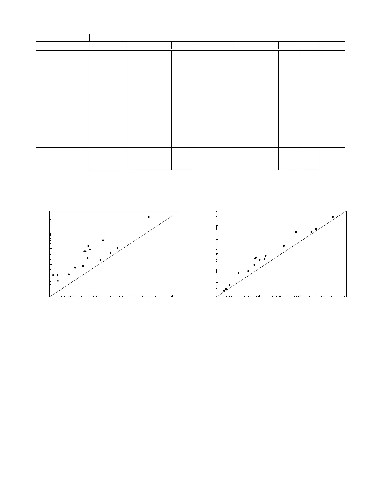
Finding Associations and Computing Similarity via Biased P air Sampling ∗ Andrea Campagna and Rasmus Pagh IT Univ ersity of Copenhagen, Denmark Email: { acam,pagh } @itu.dk Abstract —Sampling-based methods hav e pr eviously been pr o- posed f or the problem of finding interesting associations in data, even for low-support items. While these methods do not guarantee precise r esults, they can be vastly mor e efficient than approaches that rely on exact counting. However , for many similarity mea- sures no such methods have been known. In this paper we show how a wide variety of measures can be supported by a simple biased sampling method. The method also extends to find high- confidence association rules. W e demonstrate theoretically that our method is superior to exact methods when the threshold for “interesting similarity/confidence” is above the av erage pairwise similarity/confidence, and the av erage support is not too low . Our method is particularly good when transactions contain many items. W e confirm in experiments on standard association mining benchmarks that this gives a significant speedup on real data sets (sometimes much larger than the theoretical guarantees). Reductions in computation time of over an order of magnitude, and significant savings in space, are obser ved. Index T erms —algorithms; sampling; data mining; association rules. I . I N T RO D U C T I O N A central task in data mining is finding associations in a binary relation. T ypically , this is phrased in a “mark et basket” setup, where there is a sequence of baskets (from now on “transactions”), each of which is a set of items. The goal is to find patterns such as “customers who buy diapers are more likely to also buy beer”. There is no canonical w ay of defining whether an association is interesting — indeed, this seems to depend on problem-specific factors not captured by the abstract formulation. As a result, a number of measures exist: In this paper we deal with some of the most common measures, including J accar d [1], lift [2], [3], cosine , and all confidence [4], [5]. In addition, we are interested in high- confidence association rules, which are closely related to the overlap coef ficient similarity measure. W e refer to [6, Chapter 5] for general background and discussion of similarity measures. In the discussion we limit ourselves to the problem of binary associations, i.e., patterns inv olving pairs of items. There is a large literature considering the challenges of finding patterns in volving larger item sets, taking into account the aspect of ∗ This is an extended version of a paper that appeared at the IEEE International Conference on Data Mining, 2009. c  2009 IEEE. This version is superseded by a full version that can be found at http://www.itu.dk/people/pagh/papers/mining-jour.pdf , which contains stronger theoretical results and fixes a mistake in the reporting of experiments. time, multiple-lev el rules, etc. While some of our results can be extended to cover larger item sets, we will for simplicity concentrate on the binary case. Previous methods rely on one of the following approaches: 1) Identifying item pairs ( i, j ) that “occur frequently to- gether” in the transactions — in particular, this means counting the number of co-occurrences of each such pair — or 2) Computing a “signature” for each item such that the similarity of e very pair of items can be estimated by (partially) comparing the item signatures. Our approach is different from both these approaches, and generally offers improved performance and/or flexibility . In some sense we go directly to the desired result, which is the set of pairs of items with similarity measure abov e some user- defined threshold ∆ . Our method is sampling based, which means that the output may contain false positiv es, and there may be false negativ es. Howe ver , these errors are rigorously understood, and can be reduced to any desired level, at some cost of ef ficiency — our experimental results are for a false negati ve probability of less than 2%. The method for doing sampling is the main novelty of this paper , and is radically different from previous approaches that in volve sampling. The main focus in many previous association mining papers has been on space usage and the number of passes over the data set, since these have been recognized as main bottlenecks. W e believe that time has come to also carefully consider CPU time . A transaction with b items contains  b 2  item pairs, and if b is not small the ef fort of considering all pairs is non- negligible compared to the cost of reading the item set. This is true in particular if data resides in RAM, or on a modern SSD that is able to deliver data at a rate of more than a gigabyte per second. One remedy that has been used (to reduce space, but also time) is to require high support , i.e., define “occur frequently together” such that most items can be thro wn away initially , simply because they do not occur frequently enough (the y are below the support threshold ). Ho wev er , as observed in [1] this means that potentially interesting or useful associations (e.g. correlations between genes and rare diseases) are not reported. In this paper we consider the problem of finding associations without support pruning. Of course, support pruning can still be used to reduce the size of the data set before our algorithms are applied. In the following sections we first discuss the need for focusing on CPU time in data mining, and then elaborate on the relationship between our contribution and related w orks. A. I/O versus CPU In recent years, the capacity of very fast storage de vices has exploded. A typical desktop computer has 4–16 GB of RAM, that can be read (sequentially) at a speed of at least 800 million 32-bit w ords per second. The flash-based ioDri ve Duo of Fusion-io of fers up to ov er a terabyte of storage that can be read at around 400 million 32-bit words per second. Thus, ev en massiv e data sets can be read at speeds that make it challenging for CPUs to k eep up. An 8-core system must, for example, process 100 million (or 50 million) items per core per second. At 3 GHz this is 33 clock cycles (or 66 clock cycles) per item. This means that any kind of processing that is not constant time per item (e.g., using time proportional to the size of the transaction containing the item) is lik ely to be CPU bound rather than I/O bound. F or example, a hash table lookup requires on the order of 5-10 ns e ven if the hash table is L2 cache-resident (today less than 10 MB per core). This giv es an upper limit of 100-200 million lookups per second in each core, meaning that any algorithm that does more than a dozen hash table operations per item (e.g. updating the count of some item pairs) is definitely CPU bound, rather than I/O bound. In conclusion, we belie ve it is time to carefully consider optimizing internal computation time, rather than considering all computation as “free” by only counting I/Os or number of passes. Once CPU efficient algorithms are known, it is likely that the remaining bottleneck is I/O. Thus, we also consider I/O efficient versions of our algorithm. B. Pre vious work Exact counting of fr equent item sets: The approach pio- neered by the A-Priori algorithm [7], [8], and refined by many others (see e.g. [9]–[13]), allo ws, as a special case, finding all item pairs ( i, j ) that occur in more than k transactions, for a specified threshold k . Howe ver , for the similarity measures we consider, the v alue of k must in general be chosen as a low constant, since ev en pairs of very infrequent items can hav e high similarity . This means that such methods degenerate to simply counting the number of occurrences of all pairs, spending time Θ( b 2 ) on a transaction with b items. Also, generally the space usage of such methods (at least those requiring a constant number of passes ov er the data) is at least 1 bit of space for each pair that occurs in some transaction. The problem of counting the number of co-occurrences of all item pairs is in fact equi valent to the problem of multiplying sparse 0-1 matrices. T o see this, consider the n × m matrix A in which each row A i is the incidence vector having 1 in position p iff the i th element in the set of items appears in the p th transaction. Each entry ˜ A i,j of the n × n matrix ˜ A = A × A T represents the number of transactions in which the pair ( i, j ) appears. The best theoretical algorithms for (sparse) matrix multiplication [14]–[16] scale better than the A-Priori family of methods as the transaction size gets lar ger , but because of huge constant factors this is so f ar only of theoretical interest. Sampling transactions: T oiv onen [17] inv estigated the use of sampling to find candidate frequent pairs ( i, j ) : T ake a small, random subset of the transactions and see what pairs are frequent in the subset. This can considerably reduce the memory used to actually count the number of occurrences (in the full set), at the cost of some probability of missing a frequent pair . This approach is good for high-support items, but low-support associations are likely to be missed, since few transactions contain the relev ant items. Locality-sensitive hashing: Cohen et al. [1] proposed the use of another sampling technique, called min-wise indepen- dent hashing , where a small number of occurrences of each item (a “signature”) is sampled. This means that occurrences of items with low support are more likely to be sampled. As a result, pairs of (possibly low-support) items with high jaccard coefficient are found — with a probability of false positi ves and negati ves. A main result of [1] is that the time complexity of their algorithm is proportional to the sum of all pairwise jaccard coefficients, plus the cost of initially reading the data. Our main result has basically the same form, but has the advantage of supporting a wide class of similarity measures. Min-wise independent hashing belongs to the class of locality-sensitive hashing methods [18]. Another such method was described by Charikar [19], who showed how to compute succinct signatures whose Hamming distance reflects angles between incidence vectors. This leads to an algorithm for find- ing item pairs with cosine similarity above a given threshold (again, with a probability of false positiv es and negati ves), that uses linear time to compute the signatures, and Θ( n 2 ) time to find the similar pairs, where n is the number of distinct items in all transactions. Charikar also shows that many similarity measures, including some measures supported by our algorithm, cannot be handled using the approach of locality-sensitiv e hashing. Deterministic signatur e methods: In the database commu- nity , finding all pairs with similarity above a giv en threshold is sometimes referred to as a “similarity join. ” Recent results on similarity joins include [20]–[23]. While not always described in this way , these methods can be seen as deterministic analogues of the locality-sensitiv e hashing methods, of fering exact results. The idea is to avoid computing the similarity of ev ery pair by employing succinct “signatures” that may serve as witnesses for low similarity . Most of these methods require the signatures of every pair of items to be (partially) compared, which takes Ω( n 2 ) time. Howe ver , the worst-case asymptotic performance appears to be no better than the A- Priori family of methods. A similarity join algorithm that runs faster than Ω( n 2 ) in some cases is described in [20]. Howe ver , this algorithm e xhibits a polynomial dependence on the maximum number k of differences between two incidence vectors that are considered similar , and for many similarity measures the rele vant value of k may be linear in the number m of transactions. C. Our results In this paper we present a nov el sampling technique to handle a variety of measures (including jaccard, lift, cosine, and all confidence), e ven finding similar pairs among low support items. The idea is to sample a subset of all pairs ( i, j ) occurring in the transactions, letting the sampling probability be a function of the supports of i and j . For a parameter µ , the probability is chosen such that each pair with similarity abov e a threshold ∆ (an “interesting pair”) will be sampled at least µ times, in expectation, while we do not expect to see a pair ( i, j ) whose measure is significantly belo w ∆ . A na ¨ ıve implementation of this idea would still use quadratic time for each transaction, but we show how to do the sampling in near -linear time (in the size of the transaction and number of sampled pairs). The number of times a pair is sampled follows a binomial distribution, which allows us to use the sample to infer which pairs are likely to hav e similarity above the threshold, with rigorous bounds on false negati ve and false positi ve probabilities. W e show that the time used by our algorithm is (nearly) linear in the input size and in the the sum of all pairwise similarities between items, divided by the threshold ∆ . This is (close to) the best complexity one could hope for with no conditions on the distribution of pairwise similarities. Under reasonable assumptions, e.g. that the average support is not too lo w , this giv es a speedup of a factor Ω( b/ log b ) , where b is the av erage size of a transaction. W e show in extensi ve experiments on standard data sets for testing data mining algorithms that our approach (with a 1 . 8% false negati ve probability) giv es speedup factors in the vicinity of an order of magnitude, as well as significant sa vings in the amount of space required, compared to exact counting methods. W e also present e vidence that for data sets with many distinct items, our algorithm may perform significantly less work than methods based on locality-sensiti ve hashing. D. Notation Let T 1 , . . . , T m be a sequence of transactions, T j ⊆ [ n ] . For i = 1 , . . . , n let S i = { j | i ∈ T j } , i.e., S i is the set of occurrences of item i . W e are interested in finding associations among items, and consider a framework that captures the most common measures from the data mining literature. Specifically , we can handle a similarity measure s ( i, j ) if there exists a function f : N × N × R + → R + that is non-increasing in all parameters, and such that: | S i ∩ S j | f ( | S i | , | S j | , s ( i, j )) = 1 . In other words, the similarity should be the solution to an equation of the form giv en above. Fig. 1 shows particular mea- sures that are special cases. The monotonicity requirements on f hold for any reasonable similarity measure: increasing | S i ∩ S j | should not decrease the similarity , and adding an occurrence of i or j should not increase the similarity unless | S i ∩ S j | increases. In the following we assume that f is Measure s ( i, j ) f ( | S i | , | S j | , s ) lift | S i ∩ S j | | S i || S j | s − 1 m/ ( | S i | · | S j | ) cosine | S i ∩ S j | √ | S i || S j | s − 1 / p | S i | · | S j | jaccard | S i ∩ S j | | S i ∪ S j | 1+ s s / ( | S i | + | S j | ) all confidence | S i ∩ S j | max( | S i | , | S j | ) s − 1 / max( | S i | , | S j | ) dice | S i ∩ S j | | S i | + | S j | s − 1 / ( | S i | + | S j | ) ov erlap coef | S i ∩ S j | min( | S i | , | S j | ) s − 1 / min( | S 1 | , | S 2 | ) Fig. 1. Some measures cover ed by our algorithm and the corr esponding functions. Note that finding all pairs with overlap coefficient at least ∆ implies finding all association rules with confidence at least ∆ . computable in constant time, which is clearly a reasonable assumption for the measures of Fig. 1. I I . O U R A L G O R I T H M The goal is to identify pairs ( i, j ) where s ( i, j ) is “large”. Giv en a user -defined threshold ∆ we w ant to report the pairs where s ( i, j ) ≥ ∆ . W e observe that all measures in Fig. 1 are symmetric, so it suffices to find all pairs ( i, j ) where | S i | ≤ | S j | , i 6 = j , and s ( i, j ) ≥ ∆ . A. Algorithm idea Our algorithm is randomized and finds each qualifying pair with probability 1 − ε , where ε > 0 is a user-defined error probability . The algorithm may also return some false positiv es, b ut each f alse positi ve pair is lik ely to ha ve similarity within a small constant factor of ∆ . If desired, the false positiv es can be reduced or eliminated in a second phase, b ut we do not consider this step here. The basic idea is to randomly sample pairs of items that occur together in some transaction such that for any pair ( i, j ) the expected number times it is sampled is a strictly increasing function of s ( i, j ) . Indeed, in all cases e xcept the jaccard measure it is simply proportional to s ( i, j ) . W e scale the sampling probability such that for all pairs with s ( i, j ) ≥ ∆ we expect to see at least µ occurrences of ( i, j ) , where µ is a parameter (defined later) that determines the error probability . B. Implementation Fig. 2 shows our algorithm, called B I S A M (for bi ased sam pling). The algorithm iterates through the transactions, and for each transaction T t adds a subset of T t × T t to a multiset M in time that is linear in | T t | and the number of pairs added. W e use T t [ i ] to denote the i th item in T t . Because f is non-increasing and T t is sorted according to the order induced by c ( · ) we will add ( T t [ i ] , T t [ j ]) ∈ T t × T t if and only if f ( c ( T t [ i ]) , c ( T t [ j ]) , ∆) µ > r . The second loop of the algorithm builds an output set containing those pairs ( i, j ) that either occur at least µ/ 2 times in M , or where the number of occurrences in M imply that s ( i, j ) ≥ ∆ (with probability 1 ). procedur e B I S A M ( T 1 , . . . , T m ; f , µ, ∆) c := I T E M C O UN T ( T 1 , . . . , T m ) ; M := ∅ ; for t := 1 to m do sort T t [] s.t. c ( T t [ j ]) ≤ c ( T t [ j + 1]) for 1 ≤ j < | T t | ; let r be a random number in [0; 1) ; for i := 1 to | T t | do j:=i+1; while j ≤ | T t | and f ( c ( T t [ i ]) , c ( T t [ j ]) , ∆) µ > r M := M ∪ { ( T t [ i ] , T t [ j ]) } ; j:=j+1; end end end R = ∅ ; for ( i, j ) ∈ M do if M ( i, j ) > µ/ 2 or M ( i, j ) f ( c ( i ) , c ( j ) , ∆) ≥ 1 then R := R ∪ { ( i, j ) } ; retur n R ; end Fig. 2. Pseudocode for the B I S A M algorithm. The pr ocedure I T E M C O U N T ( · ) r eturns a function (hash map) that contains the number of occurr ences of each item. T t [ j ] denotes the j th item in transaction t . M is a multi set that is updated by inserting certain randomly chosen pairs ( i, j ) . The number of occurr ences of a pair ( i, j ) is denoted M ( i, j ) . The best implementation of the subprocedure I T E M C O U N T depends on the relationship between a vailable memory and the number n of distinct items. If there is suf ficient internal memory , it can be ef ficiently implemented using a hash table. For lar ger instances, a sort-and-count approach can be used (Section III-B). The multiset M can be represented using a hash table with counters (if it fits in internal memory), or more generally by an external memory data structure. In the following we first consider the standard model (often referred to as the “RAM model”), where the hash tables fit in internal memory , and assume that each insertion takes constant time. Then we consider the I/O model, for which an I/O efficient implementation is discussed. As we will show in Section IV, a sufficiently large value of µ is 8 ln(1 /ε ) . Fig. 5 sho ws more exact, concrete values of µ and corresponding false positiv e probabilities ε . Example. Suppose I T E M C O U N T has been run and the supports of items 1–6 are as sho wn in Fig. 3. Suppose now that the transaction T t = { 6 , 5 , 4 , 3 , 2 , 1 } is giv en. Note that its items are written according to the number of occurrences of each item. Assuming the similarity measure is cosine , µ = 10 , ∆ = 0 . 7 , and r for this transaction equal to 0.9, our algorithm would select from T t × T t the pairs shown in Fig. 4. Suppose that after processing all transactions the pair (6 , 5) occurs 3 times in M , (6 , 4) occurs twice in M , (6 , 1) occurs once in M , and (5 , 4) occurs 4 times in M . Then the algorithm item occurences item occurrences i c ( i ) i c ( i ) 1 60 4 5 2 60 5 5 3 50 6 3 Fig. 3. Items in the example, with corr esponding I T E M C O U N T values. i j f ( c ( i ) , c ( j ) , ∆) i j f ( c ( i ) , c ( j ) , ∆) 6 5 0.37 6 2 0.11 6 4 0.37 6 1 0.11 6 3 0.12 5 4 0.28 Fig. 4. P airs selected fr om T t in the example. Notice that after r ealizing the pair (5 , 3) does not satisfy the inequality f ( c (5) , c (3) , ∆) µ > r , the algorithm will not tak e into account the pairs (5 , 2) and (5 , 1) . would output the pairs: (6 , 5) (since M (6 , 5) < µ/ 2 but M (6 , 5) f (3 , 5 , 0 . 7) > 1 ), and (5 , 4) (same situation as before). I I I . A NA LY S I S O F R U N NI N G T I M E Our main lemma is the following: Lemma 1: For all pairs ( i, j ) , where i 6 = j and c ( i ) ≤ c ( j ) , if f ( c ( i ) , c ( j ) , ∆) µ < 1 then at the end of the procedure, M ( i, j ) has binomial distribution with | S i ∩ S j | trials and mean | S i ∩ S j | f ( | S i | , | S j | , ∆) µ. If f ( c ( i ) , c ( j ) , ∆) µ ≥ 1 then at the end of the procedure M ( i, j ) = | S i ∩ S j | . Pr oof: As observed above, the algorithm adds the pair ( i, j ) to M in iteration t if and only if ( i, j ) ∈ T t × T t and f ( c ( i ) , c ( j ) , ∆) µ > r , where r is the random number in [0; 1) chosen in iteration t . This means that for every t ∈ S i ∩ S j we add ( i, j ) to M with probability min(1 , f ( c ( i ) , c ( j ) , ∆) µ ) . In particular, M ( i, j ) = | S i ∩ S j | for f ( c ( i ) , c ( j ) , ∆) µ ≥ 1 . Otherwise, since the v alue of r is independently chosen for each t , the distribution of M ( i, j ) is binomial with | S i ∩ S j | trials and mean | S i ∩ S j | f ( c ( i ) , c ( j ) , ∆) µ . Looking at Fig. 1 we notice that for the jaccard similarity measure s ( i, j ) = | S i ∩ S j | | S i ]+ | S j |−| S i ∩ S j | , the mean of the distribu- tion is | S i ∩ S j | | S i ] + | S j | 1 + ∆ ∆ µ = µ s ( i, j )(1 + ∆) (1 + s ( i, j ))∆ ≤ 2 µ s ( i, j ) / ∆ , where the inequality uses s ( i, j ) , ∆ ∈ [0; 1] . For all other similarity measures the mean of the binomial distrib ution is µ s ( i, j ) / ∆ . As a consequence, for all these measures, pairs with similarity below (1 − ε )∆ will be counted exactly , or sampled with mean (1 − Ω( ε )) µ . Also notice that for all the measures we consider , | S i ∩ S j | f ( | S i | , | S j | , ∆) = O ( s ( i, j ) / ∆) . W e provide a running time analysis both in the standard (RAM) model and in the I/O model of Aggarwal and V it- ter [24]. In the latter case we present an external memory efficient implementation of the algorithm, I O B I S A M . Let b denote the average number of items in a transaction, i.e., there are bm items in total. Also, let z denote the number of pairs reported by the algorithm. A. Running time in the standard model The first and last part of the algorithm clearly runs in expected time O ( mb + z ) . The time for reporting the result is dominated by the time used for the main loop, but analyzing the complexity of the main loop requires some thought. The sorting of a transaction with b 1 items takes O ( b 1 log b 1 ) time, and in particular the total cost of all sorting steps is O ( mb log n ) . 1 What remains is to account for the time spent in the while loop. W e assume that | S i ∩ S j | f ( | S i | , | S j | , ∆) = O ( s ( i, j ) / ∆) , which is true for all the measures we consider . The time spent in the while loop is proportional to the number of items sampled, and according to Lemma 1 the pair ( i, j ) will be sampled | S i ∩ S j | f ( | S i | , | S j | , ∆) µ = O ( µ s ( i, j ) / ∆) times in expectation if f ( c ( i ) , c ( j ) , ∆) µ < 1 , and | S i ∩ S j | times otherwise. In both cases, the expected number of samples is O ( s ( i, j ) µ ∆ ) . Summing ov er all pairs we get the total time complexity . Theor em 2: Suppose we are given transactions T 1 , . . . , T m , each a subset of [ n ] , with mb items in total, and that f is the function corresponding to the similarity measure s . Also assume that | S i ∩ S j | f ( | S i | , | S j | , ∆) = O ( s ( i, j ) / ∆) . Then the expected time comple xity of B I S A M ( T 1 , . . . , T m ; f , µ, ∆) in the standard model is: O   mb log n + µ ∆ X 1 ≤ i r . When a pair satisfies the inequality , it is buf fered in an output page in memory , together with the item supports. Once the page is filled, it is flushed to external memory . The total cost of this phase is O ( N + N 0 B ) I/Os for the flushings and reads, where N 0 is the total number of pairs satisfying the inequality (i.e., the number of samples taken). As before, the expected v alue of N 0 is O ( µ ∆ P 1 ≤ i µ/ 2 or M ( i, j ) f ( c ( i ) , c ( j ) , ∆) ≥ 1 , which needs O ( N 0 B ) I/Os. W e observe that this cost is dom- inated by the cost of previous operations. The most expen- siv e steps are the sorting steps, whose total input has size O ( N + N 0 ) , implying that the following theorem holds: Theor em 4: Suppose we are given transactions T 1 , . . . , T m , each a subset of [ n ] , with N = mb items in total, and f is the function corresponding to the similarity measure s . Also assume | S i ∩ S j | f ( | S i | , | S j | , ∆) = O ( s ( i, j ) / ∆) . For N 0 = O ( µ ∆ P 1 ≤ i µ/ 2 . Fig. 6 illustrates two Poisson distributions (one corresponding to an item pair with measure three times belo w the threshold, and one corresponding to an item pair with measure at the threshold). Actually , the number µ/ 2 in the reporting loop of the B I S A M algorithm is just one possible choice in a range of possible trade-of fs between the number of false positi ves and false negati ves. As an alternative to increasing this threshold, a post-processing procedure may efficiently eliminate most false positiv es by more accurately estimating the corresponding values of the measure. V . V A R I A N T S A N D E X T E N S I O N S In this section we mention a number of ways in which our results can be extended. A. Alternative filtering of false positives The threshold of µ/ 2 in the B I S A M algorithms means that we filter a way most pairs whose similarity is far from ∆ . An alternativ e is to spend more time on the pairs ( i, j ) ∈ M , using a sampling method to obtain a more accurate estimate of | S i ∩ S j | . A suitable technique could be to use min-wise independent hash functions [26], [27] to obtain a sketch of Fig. 6. Illustration of false ne gatives and false positives for µ = 15 . The leftmost peak shows the pr obability distribution for the number of samples of a pair ( i, j ) with s ( i, j ) = ∆ / 3 . W ith a pr obability of ar ound 13% the number of samples is above the threshold (vertical line), which leads to the pair being r eported (false positive). The rightmost peak shows the pr obability distribution for the number of samples of a pair ( i, j ) with s ( i, j ) = ∆ . The pr obability that this is below the thr eshold, and hence not r eported (false ne gative), is ar ound 1.8%. each set S i . It suf fices to compare two sk etches in order to hav e an approximation of the jaccard similarities of S i and S j , which in turn gives an approximation of | S i ∩ S j | . Based on this we may decide if a pair is likely to be interesting, or if it is possible to filter it out. The sketches could be built and maintained during the I T E M C O U N T procedure using, say , a logaritmic number of hash functions. Indyk [27] presents an efficient class of (almost) min-wise independent hash functions. For some similarity measures such as lift and overlap coefficient the similarity of two sets may be high ev en if the sets have very dif ferent sizes. In such cases, it may be better to sample the smaller set, say , S i , and use a hash table containing the larger set S j to estimate the fraction | S i ∩ S j | / | S i | . B. Reducing space usage by using counting Bloom filters At the cost of an extra pass over the data, we may reduce the space usage. The idea, previously found in e.g. [12], is to initially create an approximate representation of M using counting Bloom filters (see [28] for an introduction). Then, in a subsequent pass we may count only those pairs that, according to the approximation, may occur at least µ/ 2 times. C. W eighted items Some applications of the cosine measure, e.g. in information retriev al, require the items to be weighted. B I S A M easily extends to this setting. D. Adaptive variant. Instead of letting ∆ be a user-defined variable, we may (informally) let ∆ go from ∞ towards 0 . This can be achieved by maintaining a priority queue of item pairs, where the priority reflects the v alue of ∆ that would allo w the pair to be sampled. Because f is non-increasing in all parameters it suffices to have a linear number of pairs from each transaction in the priority queue at any time, namely the pairs that are “next in line” to be sampled. For each of the similarity measures in Fig. 1 the value of ∆ for a pair ( i, j ) is easily computed by solving the equation f ( | S i | , | S j | , s ) µ = r for s . Decreasing ∆ corresponds to remo ving the pair with the maximum v alue from the priority queue. At any time, the set of sampled item pairs will correspond exactly to the choice of ∆ gi ven by the last pair extracted from the priority queue. The procedure can be stopped once suf ficiently many results hav e been found. E. Composite measures Notice that if f 1 ( | S i | , | S j | , ∆) and f 2 ( | S i | , | S j | , ∆) are both non-increasing, then any linear combination αf 1 + β f 2 , where α, β > 0 , is also non-increasing. Similarly , min( αf 1 , β f 2 ) is non-increasing. This allo ws us to use B I S A M to directly search for pairs with high similarity according to sev eral measures (corresponding to f 1 and f 2 ), e.g., pairs with cosine similarity at least 0 . 7 and lift at least 2 . V I . E X P E R I M E N T S T o make experiments fully reproducible and independent of implementation details and machine architecture, we focus our attention on the number of hash table operations, and the number of items in the hash tables. That is, the time for B I S A M is the number of items in the input set plus the number of pairs inserted in the multiset M . The space of B I S A M is the number of distinct items (for support counts) plus the number of distinct pairs in M . Similarly , the time for methods based on exact counting is the number of items in the input set plus the number of pairs in all transactions (since ev ery pair is counted), and the space for exact counting is the number of distinct items plus the number of distinct pairs that occur in some transaction. W e belie ve that these simplified measures of time and space are a good choice for two reasons. First, hash table lookups and updates require hundreds of clock cycles unless the relev ant key is in cache. This means that a large fraction of the time spent by a well-tuned implementation is used for hash table lookups and updates. Second, we are comparing two approaches that have a similar behavior in that they count supports of items and pairs. The key difference thus lies in the number of hash table operations, and the space used for hash tables. Also, this means that essentially any speedup or space reduction applicable to one approach is applicable to the other (e.g. using counting Bloom filters to reduce space usage). A. Data sets Experiments ha ve been run on both real datasets and artificial ones. W e hav e used most of the datasets of the Frequent Itemset Mining Implementations (FIMI) Repository 3 . In addition, we ha ve created three data sets based on the internet movie database (IMDB). 3 http://fimi.cs.helsinki.fi/ Dataset distinct number of avg . trans- max. trans- a vg. items items transactions action size action size support Chess 75 3196 37 37 1577 Connect 129 67555 43 43 22519 Mushroom 119 8134 23 23 1570 Pumsb 2113 49046 74 74 1718 Pumsb star 2088 49046 50 63 1186 K osarak 41270 990002 8 2498 194 BMS-W ebV iew-1 497 5962 2 161 301 BMS-W ebV iew-2 3340 59602 2 161 107 BMS-POS 1657 515597 6 164 2032 Retail 16470 88162 10 76 55 Accidents 468 340183 33 51 24575 T10I4D100K 870 100000 10 29 1161 T40I10D100K 942 100000 40 77 4204 actors 128203 51226 31 1002 12 directorsActor 51226 3783 1221 8887 90 movieActors 50645 133633 12 2253 33 Fig. 7. K e y figur es on the data sets used for e xperiments. The first 13 data sets ar e fr om the FIMI r epository . The last 3 wer e extracted fr om the May 29, 2009 snapshot of the Internet Movie Database (IMDB). The datasets Chess , Connect , Mushroom , Pumsb , and Pumsb star wer e pr epared by Roberto Bayar do fr om the UCI datasets and PUMBS. K osarak contains (anonymized) click-str eam data of a hungarian on-line news portal, pr ovided by F er enc Bodon. BMS-W ebView-1 , BMS-W ebV iew-2 , and BMS-POS contain clickstr eam and pur chase data of a le gwear and legcar e web r etailer , see [29] for details. Retail contains the (anonymized) r etail market basket data from a Belgian retail stor e [30]. Accidents contains (anonymized) traf fic accident data [31]. The datasets T10I4D100K and T10I4D100K have been gener ated using an IBM generator fr om the Almaden Quest resear ch gr oup. Actors contains the set of r ated movies for each male actor who has acted in at least 10 rated movies. DirectorActor contains, for each director who has dir ected at least 10 rated movies, the set of actors fr om Actors that this dir ector has worked with in rated movies. MovieActor is the in verse r elation of Actors , listing for each movie a set of actors. Fig. 7 contains some key figures on the data sets. B. Results and discussion Fig. 8 shows the results of our experiments for the co- sine measure. The time and space for B I S A M is a random variable. The reported number is an exact computation of the e xpectation of this random variable. Separate e xperiments hav e confirmed that observed time and space is relatively well concentrated around this v alue. The v alue of ∆ used is also shown — it was chosen manually in each case to gi ve a “human readable” output of around 1000 pairs. (For the IMDB data sets and the Kosarak data set this was not possible; for the latter this beha viour was due to a large number of false positiv es.) Note that choosing a smaller ∆ would bring the performance of B I S A M closer to the exact algorithms; this is not surprising, since lowering ∆ means reporting pairs having a smaller similarity measure, increasing in this way the number of samples taken. As noted before, we are usually interested in reporting pairs with high similarity , for almost an y reasonable scenario. The results for the other measures are omitted for space reasons, since they are very similar to the ones reported here. This is because the complexity of B I S A M is, in most cases, dominated by the first phase (counting item frequencies), meaning that fluctuations in the cost of the second phase hav e little effect. This also suggests that we could increase the value of µ (and possibly increase the value of the threshold µ/ 2 used in the B I S A M algorithm) without significantly changing the time complexity of the algorithm. W e see that the speedup obtained in the e xperiments v aries between a factor 2 and a factor over 30. Figures 9(a) and 9(b) giv e a graphical o vervie w . The largest speedups tend to come for data sets with the lar gest average transaction size, or data sets where some transactions are very lar ge (e.g. K osarak ). Howe ver , as our theoretical analysis suggests, large transaction size alone is not suf ficient to ensure a large speedup — items also need to have support that is not too small. So while the DirectorActor data set has very large a verage transaction size, the speedup is only moderate because the support of items is low . In a nutshell, B I S A M gives the largest speedups when there is a combination of relati vely lar ge transactions and relativ ely high a verage support. The space usage of B I S A M ranges from being quite close to the space usage for e xact counting, to a decent reduction. Though we have not experimented with methods based on locality-sensitiv e hashing (LSH), we observe that our method appears to have an advantage when the number n of distinct items is lar ge. This is because LSH in general (and in particular for cosine similarity) requires comparison of  n 2  pairs of hash signatures. For the data sets Retail , BMS- W ebview-2 , Actors , and MovieActors the ratio between the number of signature comparisons and the number of hash table operations required for B I S A M is in the range 9–265. While these numbers are not necessarily directly comparable, it does indicate that B I S A M has the potential to improve LSH-based methods that require comparison of all signature pairs. V I I . C O N C L U S I O N W e hav e presented a ne w sampling-based method for finding associations in data. Besides our initial experiments, indicating that large speedups may be obtained, there appear to be many opportunities for using our approach to implement association mining systems with very high performance. Some such opportunities are outlined in Section V, but many nontri vial aspects would hav e to be considered to do this in the best way . A C K N O W L E D G M E N T W e wish to thank Blue Martini Software for contrib uting the KDD Cup 2000 data. Also, we thank the re viewers of the ICDM submission for pointing out sev eral related works. R E F E R E N C E S [1] E. Cohen, M. Datar , S. Fujiwara, A. Gionis, P . Indyk, R. Motwani, J. D. Ullman, and C. Y ang, “Finding interesting associations without support pruning, ” IEEE T rans. Knowl. Data Eng , vol. 13, no. 1, pp. 64–78, 2001. [2] S. Brin, R. Motwani, and C. Silverstein, “Beyond market baskets: Generalizing association rules to correlations, ” SIGMOD Recor d (ACM Special Interest Group on Management of Data) , vol. 26, no. 2, pp. 265–276, Jun. 1997. [3] C. C. Aggarwal and P . S. Y u, “ A new framework for itemset generation, ” in Proceedings of the ACM SIGA CT–SIGMOD–SIGART Symposium on Principles of Database Systems (PODS ’98) . A CM Press, 1998, pp. 18–24. [4] Y .-K. Lee, W .-Y . Kim, Y . D. Cai, and J. Han, “Comine: Efficient mining of correlated patterns, ” in Pr oceedings of the IEEE International Confer ence on Data Mining (ICDM ’03) . IEEE Computer Society , 2003, pp. 581–584. [5] E. Omiecinski, “ Alternativ e interest measures for mining associations in databases, ” IEEE T rans. Knowl. Data Eng , vol. 15, no. 1, pp. 57–69, 2003. [6] J. Han and M. Kamber , Data Mining: Concepts and T echniques, 2nd edition . Morgan Kaufmann, 2006. [7] R. Agrawal, M. Mehta, J. C. Shafer, R. Srikant, A. Arning, and T . Bollinger , “The quest data mining system, ” in Proceedings of the 2nd International Conference of Knowledge Discovery and Data Mining (KDD ’96) . AAAI Press, 1996, pp. 244–249. [8] R. Agrawal and R. Srikant, “Fast algorithms for mining association rules in large databases, ” in International Confer ence On V ery Larg e Data Bases (VLDB ’94) . Morgan Kaufmann Publishers, Inc., Sep. 1994, pp. 487–499. [9] FIMI ’03, Proceedings of the ICDM 2003 W orkshop on Fr equent Itemset Mining Implementations , ser . CEUR W orkshop Proceedings, vol. 90. CEUR-WS.org, 2003. [10] FIMI ’04, Proceedings of the IEEE ICDM W orkshop on F requent Itemset Mining Implementations , ser . CEUR W orkshop Proceedings, vol. 126. CEUR-WS.org, 2004. [11] S. Brin, R. Motwani, J. D. Ullman, and S. Tsur , “Dynamic itemset counting and implication rules for market basket data, ” in Proceedings of the ACM-SIGMOD International Conference on Management of Data (SIGMOD ’97) , ser . SIGMOD Record (ACM Special Interest Group on Management of Data), vol. 26(2). ACM Press, 1997, pp. 255–264. [12] J. S. Park, M.-S. Chen, and P . S. Y u, “ An effecti ve hash-based algorithm for mining association rules, ” SIGMOD Record (ACM Special Inter est Gr oup on Management of Data) , vol. 24, no. 2, pp. 175–186, Jun. 1995. [13] A. Savasere, E. Omiecinski, and S. B. Nav athe, “ An efficient algorithm for mining association rules in large databases, ” in Proceedings of the 21st International Conference on V ery Larg e Data Bases (VLDB ’95) . Morgan Kaufmann Publishers, 1995, pp. 432–444. [14] R. R. Amossen and R. Pagh, “Faster join-projects and sparse matrix multiplications, ” in Database Theory - ICDT 2009, 12th International Confer ence, St. P etersbur g, Russia, Mar ch 23-25, 2009, Proceedings , ser . ACM International Conference Proceeding Series, vol. 361. ACM, 2009, pp. 121–126. [15] D. Coppersmith and S. W inograd, “Matrix multiplication via arithmetic progressions, ” J. Symb . Comput. , vol. 9, no. 3, pp. 251–280, 1990. [16] R. Y uster and U. Zwick, “Fast sparse matrix multiplication, ” ACM T rans. Algorithms , vol. 1, no. 1, pp. 2–13, 2005. [17] H. T oivonen, “Sampling large databases for association rules, ” in Pro- ceedings of the 22nd International Confer ence on V ery Lar ge Data Bases (VLDB ’96) . Morgan Kaufmann Publishers, 1996, pp. 134–145. [18] P . Indyk, R. Motwani, P . Raghav an, and S. V empala, “Locality- preserving hashing in multidimensional spaces, ” in Pr oceedings of the T wenty-Ninth Annual ACM Symposium on Theory of Computing , 4–6 May 1997, pp. 618–625. [19] M. S. Charikar, “Similarity estimation techniques from rounding al- gorithms, ” in STOC ’02: Pr oceedings of the thiry-fourth annual A CM symposium on Theory of computing . ACM, 2002, pp. 380–388. [20] A. Arasu, V . Ganti, and R. Kaushik, “Efficient exact set-similarity joins, ” in VLDB . ACM, 2006, pp. 918–929. [21] S. Chaudhuri, V . Ganti, and R. Kaushik, “ A primitive operator for similarity joins in data cleaning, ” in ICDE . IEEE Computer Society , 2006, p. 5. [22] C. Xiao, W . W ang, X. Lin, and H. Shang, “T op-k set similarity joins, ” in Pr oceedings of the 25th International Conference on Data Engineering, (ICDE ’09) . IEEE, 2009, pp. 916–927. [23] C. Xiao, W . W ang, X. Lin, and J. X. Y u, “Ef ficient similarity joins for near duplicate detection, ” in Proceedings of the 17th International Confer ence on W orld W ide W eb, (WWW ’08) . ACM, 2008, pp. 131–140. Time Space Dataset B I S A M Exact counting Ratio B I S A M Exact counting Ratio ∆ #output Chess 1 . 39 · 10 5 22 . 5 · 10 5 16.21 2 . 27 · 10 3 2 . 66 · 10 3 1.17 0.6 1039 Connect 29 . 3 · 10 5 639 · 10 5 21.82 4 . 21 · 10 3 6 . 96 · 10 3 1.65 0.7 1025 Mushroom 2 . 07 · 10 5 22 . 4 · 10 5 10.84 2 . 89 · 10 3 6 . 29 · 10 3 2.18 0.4 976 Pumsb 37 . 7 · 10 5 1360 · 10 5 36.14 67 . 8 · 10 3 536 · 10 3 7.91 0.7 3070 Pumsb star 25 . 8 · 10 5 638 · 10 5 24.74 60 . 9 · 10 3 485 · 10 3 7.95 0.7 1929 K osarak 148 · 10 5 3130 · 10 5 21.13 4790 · 10 3 33100 · 10 3 6.92 0.95 63500 BMS-W ebV iew-1 2 . 19 · 10 5 9 . 64 · 10 5 4.40 29 . 7 · 10 3 64 . 5 · 10 3 2.17 0.4 1226 BMS-W ebV iew-2 6 . 03 · 10 5 24 . 4 · 10 5 4.04 188 · 10 3 725 · 10 3 3.86 0.6 1317 BMS-POS 35 . 3 · 10 5 246 · 10 5 6.96 99 . 8 · 10 3 381 · 10 3 3.82 0.15 1263 Retail 23 · 10 5 80 . 7 · 10 5 3.50 1300 · 10 3 3600 · 10 3 2.78 0.3 1099 Accidents 115 · 10 5 187 · 10 5 1.62 10 . 9 · 10 3 47 . 3 · 10 3 4.35 0.5 995 T10I4D100K 11 · 10 5 62 . 8 · 10 5 5.72 57 . 8 · 10 3 171 · 10 3 2.95 0.4 846 T40I10D100K 42 . 6 · 10 5 841 · 10 5 19.74 168 · 10 3 433 · 10 3 2.57 0.5 1120 Actors 301 · 10 5 500 · 10 5 1.66 24100 · 10 3 32900 · 10 3 1.37 0.5 18531 DirectorsActor 10700 · 10 5 81500 · 10 5 7.64 236000 · 10 3 367000 · 10 3 1.56 0.5 — MovieActors 581 · 10 5 1070 · 10 5 1.84 38900 · 10 3 55400 · 10 3 1.42 0.5 43567 Fig. 8. Result of e xperiments for the cosine measure and µ = 15 (which gives false negative pr obability 1.8%). #output is the number of pairs of items reported; ∆ is the thr eshold for “interesting similarity . ” Dir ectorsActor lacks the output because of the huge number of pairs. 100000 1 x 10 6 1 x 10 7 1 x 10 8 1 x 10 9 1 x 10 10 Time for BiSam 100000 1 x 10 6 1 x 10 7 1 x 10 8 1 x 10 9 1 x 10 10 Time for exact counting (a) Comparison of the time for B I S A M and for e xact count- ing in all experiments. The line is the identity function. T ypical dif fer ence is about an or der of magnitude. 1000 10000 100000 1 x 10 6 1 x 10 7 1 x 10 8 1 x 10 9 Space for BiSam 1000 10000 100000 1 x 10 6 1 x 10 7 1 x 10 8 1 x 10 9 Space for exact counting (b) Comparison of the space for B I S A M and for exact counting in all experiments. The line is the identity function. Fig. 9. Space and time comparisons [24] A. Aggarwal and J. S. V itter , “The input/output complexity of sorting and related problems, ” Comm. A CM , vol. 31, no. 9, pp. 1116–1127, 1988. [25] R. Motw ani and P . Raghav an, Randomized algorithms . Cambridge Univ ersity Press, 1995. [26] A. Z. Broder, M. Charikar, A. M. Frieze, and M. Mitzenmacher, “Min- wise independent permutations, ” J . Comput. Syst. Sci. , vol. 60, no. 3, pp. 630–659, 2000. [27] P . Indyk, “ A small approximately min-wise independent family of hash functions, ” in Pr oocedings of the 10th Annual ACM-SIAM Symposium on Discrete Algorithms (SODA ’99) , 1999, pp. 454–456. [28] A. Z. Broder and M. Mitzenmacher, “Network applications of Bloom filters: A surve y , ” in Pr oceedings of the 40th Annual Allerton Confer ence on Communication, Contr ol, and Computing . A CM Press, 2002, pp. 636–646. [29] R. Koha vi, C. Brodley , B. Frasca, L. Mason, and Z. Zheng, “KDD- Cup 2000 organizers’ report: Peeling the onion, ” SIGKDD Explorations , vol. 2, no. 2, pp. 86–98, 2000. [30] T . Brijs, G. Swinnen, K. V anhoof, and G. W ets, “Using association rules for product assortment decisions: A case study , ” in Pr oceedings of the F ifth ACM SIGKDD International Conference on Knowledge Discovery and Data Mining (KDD ’99) . ACM Press, 1999, pp. 254–260. [31] K. Geurts, G. W ets, T . Brijs, and K. V anhoof, “Profiling high frequency accident locations using association rules, ” in Proceedings of the 82nd Annual T ransportation Researc h Board , 2003, p. 18pp.