New exact multi line soliton and periodic solutions with constant asymptotic values at infinity of the NVN integrable nonlinear evolution equation via dibar-dressing method

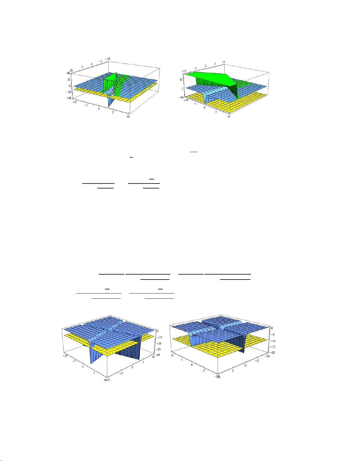
New exact solutions with constan t asymptotic v a lues at inﬁnit y of the NVN in tegrable nonlinear ev olution equation via ¯ ∂ -dressing metho d M.Y u. Ba salaev, V.G. Dubro vsky and A.V. T opovsky Nov osibirsk State T ec hnical Unive rsity , Karl Marx prosp. 20, Nov osi birsk 630092, Russi a E-mail: dubro vsky@aca dem.org Abstract. The classes of exact multi line sol i to n, peri odic solutions and solutions with functional par ameters, with constan t asymptotic v alues at inﬁnity u | ξ 2 + η 2 →∞ → − ǫ , for the h yperb olic and elliptic versions of the Nizhnik-V eselov- Nov iko v (NVN ) equation via ¯ ∂ -dressing method of Zakharo v and Manako v were constructed. At ﬁxed tim e these solutions are exactly solv able p ote n tials corresp ond ingly for one-dimensional p erturbed telegraph and tw o-di men sional stationary Sc hr¨ odinger equations. Ph ysical meaning of stationary states of quantum particle in exact one li ne and t wo line soliton p ot en tial v alleys was di s c ussed. In the li mit ǫ → 0 exact special solutions u (1) , u (2) (line soli tons and p eriodic solutions) were found which sum u (1) + u (2) (linear sup e rp osition) is also exact solution of NVN equation. P ACS num b ers: 02.30 .Ik, 02.30.Jr , 02.30.Zz, 05.45.Yv 1. In tro duction Exact solutions of diﬀeren tial equations o f mathematical physics, linear and nonlinear, are very imp ortan t for the understanding of v arious ph ysical phenomena. In the la st three decades the Inv erse Sca t tering T ransform (IST) metho d has b een g eneralized and successfully applied to several t wo-dimensional nonlinear evolution equa tio ns such as Kadomtsev-Petviash vili, Dav ey - Stew arts o n, Nizhnik-V eselov-No vikov, Zakharov- Manako v system, Ishimo r i, t wo-dimensional integrable Sin-Gordon and others (see bo oks [1]-[4] a nd references therein). The extension of nonloca l Riemann-Hilb ert pro blem b y Zakharov and Manako v [5 ] and ¯ ∂ -pro blem a pproac h [6] led to the discov ery of more genera l ¯ ∂ -dressing method [7]- [10] whic h became very pow er f ul method for solving t w o-dimensional in tegrable nonlinear evolution eq ua tions. In the present pap er the ¯ ∂ -dres s ing metho d of Z akharov and Manakov was used for the constructio n of the classes o f exac t multisoliton and per iodic solutions of the famous (2+1)-dimensio nal Nizhnik- V e s elo v- No vikov (NVN) int egrable e q uation u t + κ 1 u ξξ ξ + κ 2 u ηη η + 3 κ 1 ( u∂ − 1 η u ξ ) ξ + 3 κ 2 ( u∂ − 1 ξ u η ) η = 0 , (1.1) where u ( ξ , η, t ) is sca la r function, κ 1 , κ 2 are arbitrary constants, ξ = x + σ y, η = x − σy , and σ 2 = ± 1; ∂ ξ ≡ ∂ ∂ ξ , ∂ η ≡ ∂ ∂ η and ∂ − 1 ξ , ∂ − 1 η are op erators inv erse to ∂ ξ and ∂ η : New exact solut i ons of the NV N nonline ar e quation via ¯ ∂ -dr essing metho d 2 ∂ − 1 η ∂ η = ∂ − 1 ξ ∂ ξ = 1. Equa tion (1.1) was ﬁrst intro duced and studied by Nizhnik [11] for hyperb olic v er sion (NVN-I I e q uation) with σ = 1 a nd indep enden tly by V eselov and Novik ov [1 2 ] for elliptic version (NVN-I equation) with σ = i , κ 1 = κ 2 = κ . The NVN equation is in tegrable by the IST due to represe ntation o f it as the compatibility condition fo r tw o linea r auxiliary problems [11],[12]: L 1 ψ =  ∂ 2 ξη + u  ψ = 0 , (1.2) L 2 ψ =  ∂ t + κ 1 ∂ 3 ξ + κ 2 ∂ 3 η + 3 κ 1  ∂ − 1 η u ξ  + 3 κ 2  ∂ − 1 ξ u η  ψ = 0 (1.3) in the form of the Manakov’s tria d [ L 1 , L 2 ] = B L 1 , B = 3  κ 1 ∂ − 1 η u ξξ + κ 2 ∂ − 1 ξ u ηη  . (1.4) The present pa per is the con tin uation of Dubrovsky e t al w o rk a nd follo ws the notations, review of the sub ject a nd ge neral considera tions presented in the previous pap ers [22]-[24]. W e apply the ¯ ∂ -dres s ing metho d of Zakharov and Manako v for the construction of classes of exa ct solutions with non-zero constant asymptotic v alues at inﬁnit y: u ( ξ , η , t ) = ˜ u ( ξ , η, t ) + u ∞ = ˜ u ( ξ , η , t ) − ǫ, (1.5) where ˜ u ( ξ, η , t ) → 0 as ξ 2 + η 2 → ∞ . In this ca se the ﬁrst linear aux ilia ry problem in (1.2) ha s the fo r m:  ∂ 2 ξη + ˜ u  ψ = ǫψ . (1.6) F or σ = 1 with rea l spa ce v ariables ξ ⇒ t − x, η ⇒ t + y equation (1.6) can be int erpreted as per turbed telegraph eq uation with p oten tial u = ˜ u − ǫ or p erturbe d string equa tion for ǫ = 0. F or σ = i with co mplex spa ce v aria bles ξ ⇒ x + i y = z , η ⇒ x − iy = z equation (1.6) co incides with the famous tw o-dimens io nal stationary Schr¨ odinger equation  − 2 ∂ 2 z ¯ z + V S chr  ψ = E ψ (1.7) with V S chr = − 2 ˜ u and E = − 2 ǫ . F or this reas on the cons tr uction v ia ¯ ∂ -dressing metho d of exact so lut ions o f the NVN equations with c o nstan t asymptotic v alues at inﬁnit y mea ns simultaneous calculation of exact eigenfunctions (wa ve functions ) ψ and exactly solv able potentials u = ˜ u − ǫ and V S chr = − 2 ˜ u for ab ov e men tioned famous linear equa tio ns. The inv erse scattering tra ns f orm for the ﬁrst a ux iliary linear problem (1.6) (or in particular for 2D Sc hr ¨ o dinger equatio n (1.7)) has been de velop ed in a num b er of pap ers. Detailed review o ne can ﬁnd in the b oo k of K o nopelchenk o [3]. On the basis of developed for (1.6) IST using time evolution given by second aux ilia ry pr o blem (1.3) several classes of exact s o lutions of NVN equation were constr ucted [3], [4],[11]-[2 1 ]. Some exa c t so lutions o f NVN-I I equation with σ = 1 were obtained in the work [11] via the transformation oper ators. V eselov et al constructed ﬁnite zone solutions of NVN eq uation [12]. The clas ses of r ational lo calized solutions of so called N V N − I ± - equation (with E > 0 and E < 0 for (1.7)) corr e sponding to the case of simple p oles of w av e function ψ were presented in the works [14]- [16 ]. Spec ia l care requires the case of E = 0 for (1.7), i. e. the c ase of N V N − I 0 equation [17]. The use o f Darbu transformatio ns for the construction of exact so lutions of NVN equation w a s demonstrated by Matveev et al [18]. The cla ss of dromion-like solutions of NVN equation via Mottard transforma t ions was c o nstructed b y Athorne et al [21]. W e hav e already constr ucted classes of ex act p oten tia ls for p erturbed telegraph equatio n (1.6) New exact solut i ons of the NV N nonline ar e quation via ¯ ∂ -dr essing metho d 3 with potential u = ˜ u − ǫ a nd p erturbe d str ing equation with u = ˜ u, ǫ = 0 via ∂ - dressing metho d in the pap er [22] a nd obtained so me r ationally lo calized solutions of NVN-equation with simple and mult iple p ole wa ve functions ψ via ∂ -dressing metho d [23],[24]. Present work is concentrated on further use of ∂ -dres s ing method fo r the construction of exact solutions of t wo-dimensional int egrable nonlinear evolution equations, exact p oten tials and wa ve functions of famous linear a ux iliary pr oblems (1.6) o r (1.7) and the study of their po ssible applications. While many studies of this sub ject w ere perfor med the question of physical in terpr etation and exploitation of re s ults obtained via ∂ -dres s ing are still of grea t interest. The pap er is o rganized as des c r ibed further. Basic ingr edien ts of the ¯ ∂ -dressing metho d for the NVN equa tion (1.1) in brief are pr esen ted in sectio ns 2,3 and gener al determinant fo rm ula for multi line so liton solutio ns and useful for m ulas for the conditions of rea lity and p oten tiality of u a re obtained. In sections 4 and 5 the classes of exact multi line s o liton s olutions for h yp erbolic version with σ = 1 and for e llipt ic version with σ = i of the NVN equa tion resp ectively are constructed. The cla sses of p erio dic solutions for bo th v ersions of NVN equation a re constructed in section 6. The clas ses o f so lutions with functional parameter s are c o nstructed in s ection 7. The simplest exa mples of exact one, tw o line soliton solutions with corresp onding exact wa ve functions of auxiliary linear problems, per iodic solutions and solutions with functional parameter s a r e presented in sections 3,4 and 5 ,6,7 of the pap er. 2. Basic ingredien ts of the ¯ ∂ -dressi ng m ethod and general determ i nan t form ulas for exac t solutio ns As a matter of conv enience here we brieﬂy rev ie wed the ba s ic ingredien ts of the ¯ ∂ - dressing metho d [7]- [10] for the NVN equa t ion (1.1) in the case of u ( ξ , η , t ) with generically non-zer o asy mpt otic v alue at inﬁnity (1.6). W e follow ed the trea tment o f the pap ers [23],[24] witho ut rep etition of theirs detailed calcula tions. A t ﬁrst one p ostulates the no n- local ¯ ∂ -pro blem: ∂ χ ( λ, ¯ λ ) ∂ ¯ λ = ( χ ∗ R )( λ, ¯ λ ) = Z Z C χ ( µ, µ ) R ( µ, µ ; λ, ¯ λ ) dµ ∧ dµ (2.1) where in o ur case χ a nd R are the scalar c omplex-v alue d functions and χ has canonical normalizatio n: χ → 1 as λ → ∞ . It should b e ass umed that the problem (2.1) is unique solv able. Then one in tro duces the dependence of kernel R of the ¯ ∂ -pro blem (2.1) o n the spa ce and time v ariables ξ , η , t : ∂ R ∂ ξ = iµR ( µ, µ ; λ, λ ; ξ , η, t ) − R ( µ, µ ; λ, λ ; ξ , η , t ) iλ, ∂ R ∂ η = − i ǫ µ R ( µ, µ ; λ, λ ; ξ , η , t ) + R ( µ, µ ; λ, λ ; ξ , η , t ) i ǫ λ , (2.2) ∂ R ∂ t = i ( κ 1 µ 3 − κ 2 ǫ 3 µ 3 ) R ( µ, µ ; λ, λ ; ξ , η , t ) − R ( µ, µ ; λ, λ ; ξ , η , t ) i ( κ 1 λ 3 − κ 2 ǫ 3 λ 3 ) . Int egrating (2.2) one obta ins R ( µ, µ ; λ, ¯ λ ; ξ , η , t ) = R 0 ( µ, µ ; λ, ¯ λ ) e F ( µ ; ξ, η ,t ) − F ( λ ; ξ , η,t ) (2.3) where F ( λ ; ξ , η , t ) = i  λξ − ǫ λ η +  κ 1 λ 3 − κ 2 ǫ 3 λ 3  t  . (2.4) New exact solut i ons of the NV N nonline ar e quation via ¯ ∂ -dr essing metho d 4 By the use of ”long” deriv atives D 1 = ∂ ξ + iλ, D 2 = ∂ η − i ǫ λ , D 3 = ∂ t + i  κ 1 λ 3 − κ 2 ǫ 3 λ 3  (2.5) expressing the dep endence (2 .2) of kernel R o f the ¯ ∂ -pro blem (2.1 ) on the space and time v ar iables ξ , η , t in the following equiv a len t form [ D 1 , R ] = 0 , [ D 2 , R ] = 0 , [ D 3 , R ] = 0 (2.6) one can construct the op erators of auxiliary linear problems ˜ L = X l,m,n u lmn ( ξ , η , t ) D l 1 D m 2 D n 3 . (2.7) These o perator s must s a tisfy to the conditions h ∂ ∂ λ , ˜ L i χ = 0 , ˜ Lχ ( λ, λ ) | λ →∞ → 0 (2.8) of a bsence singularities at the po in ts λ = 0 and λ = ∞ o f the complex plane of sp ectral v ariable λ . F or suc h oper ators ˜ L the function ˜ Lχ obeys the same ¯ ∂ -equatio n as the function χ . There ar e may b e several op erators ˜ L i of this type, b y virtue of the unique solv ability of (2.1) one has ˜ L i χ = 0 for each of them. In considered case o ne constr ucts t wo such o perators : ˜ L 1 = D 1 D 2 + u 1 D 1 + u 2 D 2 + u, (2.9) ˜ L 2 = D 3 + κ 1 D 3 1 + κ 2 D 3 2 + V 1 D 2 1 + V 2 D 2 2 + V 3 D 1 + V 4 D 2 + V . (2.10) Using the c o nditions (2 .8 ) and se ries expa ns ions of wa ve functions χ near the p oint s λ = 0 and λ = ∞ χ = χ 0 + χ 1 λ + χ 2 λ 2 + . . . , χ = χ ∞ + χ − 1 λ + χ − 2 λ 2 + . . . , (2.11) one obtains the rec o nstruction for m ulas for the ﬁeld v a riables u 1 , u 2 and V 1 , V 2 , V 3 , V 4 through the co eﬃcients χ 0 and χ ∞ of expansions (2.1 1 ) (for calculation details s ee pap ers [2 3],[24]): u 1 = − χ ∞ η χ ∞ , V 1 = − 3 κ 1 χ ∞ ξ χ ∞ ; (2.12) u 2 = − χ 0 ξ χ 0 , V 2 = − 3 κ 2 χ 0 η χ 0 ; (2.13) V 3 = 3 iκ 2 ǫχ 1 η , V 4 = − 3 i κ 1 χ − 1 ξ . (2.14) According to well k nown terminology the op erator ˜ L 1 in (2.9 ) is pure p otential op erator when its ﬁr st deriv a tives are a bsen t. Due to canonical normaliza tio n of wav e function χ | λ →∞ → 1 ( χ ∞ = 1): u 1 = − χ ∞ η χ ∞ = 0 , V 1 = − 3 κ 1 χ ∞ ξ χ ∞ = 0 . (2.15) F or zero v alue o f the term u 2 ∂ η in ˜ L 1 one must to r equire χ 0 = const , witho ut restriction we can choo se χ 0 = 1, a nd then due to (2 .13 ) u 2 = − χ 0 ξ χ 0 = 0 , V 2 = − 3 κ 2 χ 0 η χ 0 = 0 . (2.16) Using (2.8),(2.12) - (2 .16) (for calculation de ta ils see also [23],[24]) o ne obtains the following expr essions for V 3 , V 4 and u : V 3 = 3 iκ 2 ǫχ 1 η = 3 κ 2 ∂ − 1 ξ u η , V 4 = − 3 i κ 1 χ − 1 ξ = 3 κ 1 ∂ − 1 η u ξ , (2.17) New exact solut i ons of the NV N nonline ar e quation via ¯ ∂ -dr essing metho d 5 u = − ǫ − iχ − 1 η = − ǫ + i ǫχ 1 ξ . (2.18) The ﬁeld v ariable V in (2.10) due to gaug e fr eedom [25] in the pr e s en t pap er is chosen to b e equal to zero. In terms of the wav e function ψ := χe F ( λ ; ξ, η ,t ) = χe i  λξ − ǫ λ η +  κ 1 λ 3 − κ 2 ǫ 3 λ 3  t  , (2.19) under the reduction u 1 = 0 and u 2 = 0 (the condition o f p otent iality ˜ L 1 ), one obtains from (2 .9),(2.10) due to (2.8) and (2.15)-(2.17) the linear auxiliary system (1 .2),(1.3) and NVN integrable nonlinear eq ua tion (1.1) as co mpatibilit y c o ndition (1.4) of linear auxiliary pro ble ms in (1.2), (1.3). The solution of the ¯ ∂ -pro blem (2.1) with co nstan t nor malization χ ∞ = 1 is equiv alent to the so lution of the following sing ular integral equation: χ ( λ ) = 1 + Z Z C dλ ′ ∧ d ¯ λ ′ 2 π i ( λ ′ − λ ) Z Z C χ ( µ, ¯ µ ) R ( µ, µ ; λ, ¯ λ ) dµ ∧ d ¯ µ. (2.20) F rom (2.2 0) one o bta ins for the co eﬃcien ts χ 0 and χ − 1 of the s eries expansio ns (2.11) of χ the following e xpressions: χ 0 = 1 + Z Z C dλ ∧ d ¯ λ 2 π iλ Z Z C χ ( µ, ¯ µ ) R 0 ( µ, µ ; λ, ¯ λ ) e F ( µ ) − F ( λ ) dµ ∧ d ¯ µ (2.21) and χ − 1 = − Z Z C dλ ∧ d ¯ λ 2 π i Z Z C χ ( µ, ¯ µ ) R 0 ( µ, µ ; λ, ¯ λ ) e F ( µ ) − F ( λ ) dµ ∧ d ¯ µ (2.22) where F ( λ ) is short notation for F ( λ ; ξ , η , t ) given b y the formula (2.4). The co nditions of r e a lit y u a nd of p oten tiality of the op erator ˜ L 1 give some r estrictions for the kernel R 0 of the ¯ ∂ -problem (2.1 ). In the Nizhnik case ( σ = 1 , ¯ κ 1 = κ 1 , ¯ κ 2 = κ 2 ) of the NVN equations (1.1) with rea l space v ar iables ξ = x + y , η = x − y the condition of r ealit y of u leads from (2.18) and (2.22) in the limit of ” w eak” ﬁelds ( χ = 1 in (2.22)) to the following re striction for the kernel R 0 of the ¯ ∂ - problem: R 0 ( µ, µ ; λ, λ ) = R 0 ( − µ, − µ ; − λ, − λ ) . (2.23) F or the V eselov-No viko v case ( σ = i, κ 1 = κ 2 = κ = ¯ κ ) of the NVN equations (1.1) with complex space v ar ia bles ξ = z = x + iy , η = ¯ z = x − i y the condition o f r e a lit y of u lea ds from (2.18) and (2 .2 2) in the limit of ”weak” ﬁelds to another restriction on the kernel R 0 of the ¯ ∂ - problem: R 0 ( µ, µ ; λ, λ ) = ǫ 3 | µ | 2 | λ | 2 µλ R 0 ( − ǫ λ , − ǫ λ , − ǫ µ − ǫ µ ) . (2.24) The potentialit y condition for the oper ator ˜ L 1 in (2.9) for the choice χ 0 = 1 due to (2.21) has the following form: χ 0 − 1 = Z Z C dλ ∧ d λ 2 π iλ Z Z C χ ( µ, µ ) R 0 ( µ, µ ; λ, λ ) e F ( µ ) − F ( λ ) dµ ∧ dµ = 0 . (2.25) Here we obtained gene r al formulas for multisoliton solutions corr esponding to the degenerate delta -k er nel R 0 : R 0 ( µ, ¯ µ ; λ, ¯ λ ) = π X k A k δ ( µ − M k ) δ ( λ − Λ k ) . (2.26 ) New exact solut i ons of the NV N nonline ar e quation via ¯ ∂ -dr essing metho d 6 In this case the wa ve function χ ( λ ) due to (2.20) has the for m: χ ( λ ) = 1 + 2 i X k A k Λ k − λ χ ( M k ) e F ( M k ) − F (Λ k ) . (2.27) The co eﬃcient χ − 1 due to (2 .2 2 ) and (2.26) ha s the for m: χ − 1 = − 2 i X k A k χ ( M k ) e F ( M k ) − F (Λ k ) . (2.28) F or the wa ve functions χ ( M k ) from (2 .27) one obtains the following system of equations: X l ˜ A kl χ ( M l ) = 1 , ˜ A lk = δ lk + 2 iA k M l − Λ k e F ( M k ) − F (Λ k ) . (2.29) Instead of matrix ˜ A in (2.2 9 ) it is conv enient to intro duce ma trix A given b y expression A lk = δ lk + 2 iA k M l − Λ k e F ( M l ) − F (Λ k ) . (2.30) Both these matrices ˜ A in (2.29) and A (7.19) a r e connected by the re la tion A lk = e F ( M l ) ˜ A lk e − F ( M k ) . (2.31) F rom (2.29) due to (2.31) one derives the ex pr ession for the wa ve function χ at discrete v alues of sp ectral v a riable: χ ( M l ) = X k ˜ A − 1 lk = X k e F ( M k ) − F ( M l ) A − 1 lk . (2.32) As a matter of conv enience hereafter we descr ibed some useful formulas for wav e functions sa tisfying to linear auxilia r y pro blems (1.2),(1.3). F rom (2.19) and (2 .32 ) one o btains the wa v e function ψ ( M l , ξ , η , t ) = χ ( M l ) e F ( M l ) at discr ete p oin ts λ = M l in the space of sp ectral v a riables: ψ ( M l , ξ , η , t ) = χ ( M l ) e F ( M l ) = X k e F ( M k ) A − 1 lk . (2.33) F or the wav e function (2.1 9 ) at arbitrar y po in t λ from (2.2 7 ) - (2.32) follows the expression: ψ ( λ, ξ , η , t ) = χ ( λ ) e F ( λ ) = h 1 + 2 i X k A k Λ k − λ e F ( M k ) − F (Λ k ) χ ( M k ) i e F ( λ ) = h 1 + 2 i X k,l A k Λ k − λ e − F (Λ k ) A − 1 kl e F ( M l ) i e F ( λ ) . (2.34) Inserting (2.3 2) int o (2.28) one obtains for the co eﬃcien t χ − 1 χ − 1 = − 2 i X k,l A k e F ( M k ) − F (Λ k ) e F ( M l ) − F ( M k ) A − 1 kl = = − 2 i X k,l A k e F ( M l ) − F (Λ k ) A − 1 kl = i tr  ∂ A ∂ ξ A − 1  . (2.35) and due to reconstruction formula u = − ǫ − iχ − 1 η the conv enien t determina nt formula for the solution u of NVN equation (1.1): u = − ǫ + ∂ ∂ η tr  ∂ A ∂ ξ A − 1  = − ǫ + ∂ 2 ∂ ξ ∂ η ln(det A ) . (2.36) New exact solut i ons of the NV N nonline ar e quation via ¯ ∂ -dr essing metho d 7 Here a nd b elo w useful determinant identities T r ( ∂ A ∂ ξ A − 1 ) = ∂ ∂ ξ ln(det A ) , 1 + tr D = det (1 + D ) (2.37) are used; the matrix D from las t identit y of (7.12) is degenera te with r ank 1. Poten tiality condition (2.25) by the use of (2.26)-(2.3 2) c a n b e transfor med to the form: χ 0 − 1 = − 1 2 ǫ N X k,l =1 A − 1 kl B lk = 0 (2.38) where degener ate matrix B with rank 1 is deﬁned by the for m ula B lk = − 4 iǫ Λ k A k e F ( M l ) − F (Λ k ) . (2.39) Due to (7.12)-(7.20) p otent iality condition (2 .25) takes the for m: 0 = N X k,m =1 A − 1 km B mk = tr ( A − 1 B ) = det ( B A − 1 + 1) − 1 , (2.40) here matr ix B A − 1 is degener ate of rank 1 and in deriving the last equality in (7.16) the second matrix identit y of (7.1 2 ) is used. Equiv alently due to (7.16) the p oten tiality condition ta k es the fo rm det( A + B ) = det A. (2.41) 3. F ulﬁlmen t of p oten tialit y conditi o n. General formulas for one line and t wo line so litons F ormula (2.3 6 ) for exa c t solutions u ( ξ , η , t ) of NVN equa tions (1.1) is eﬀectiv e if the reality ¯ u = u conditions (2 .23 ),(2.2 4) a nd po tentiality co nditio n (2.2 5) of op erator L 1 are sa tisﬁed. This is the ma jor and the mo st diﬃcult part o f all constructions. Here we demonstrated how one can to fulﬁl the condition of p otent iality (2.25) by delta-kernel with tw o terms: R 0 ( µ, ¯ µ ; λ, ¯ λ ) = π  Aδ ( µ − µ 1 ) δ ( λ − λ 1 ) + B δ ( µ − µ 2 ) δ ( λ − λ 2 )  . (3.1) Inserting (3.1 ) into (2.25) one obtains in the limit of weak ﬁelds ( χ = 1 in (2.25)): χ 0 − 1 = Z Z C 1 2 iλ  Aδ ( µ − µ 1 ) δ ( λ − λ 1 ) + B δ ( µ − µ 2 ) δ ( λ − λ 2 )  × × e F ( µ ) − F ( λ ) dµ ∧ d µ dλ ∧ dλ = 2 i  A λ 1 e F ( µ 1 ) − F ( λ 1 ) + B λ 2 e F ( µ 2 ) − F ( λ 2 )  = 0 . (3.2) The equa lit y (3.2) is v alid if F ( µ 1 ) − F ( λ 1 ) = F ( µ 2 ) − F ( λ 2 ) , A λ 1 = − B λ 2 . (3.3) Due to the deﬁnition of F ( λ ) = i  λξ − ǫ λ η +  κ 1 λ 3 − κ 2 ǫ 3 λ 3  t  from space-dep enden t part of (3.3) the s ystem o f equations follows: µ 1 − λ 1 = µ 2 − λ 2 , ǫ µ 1 − ǫ λ 1 = ǫ µ 2 − ǫ λ 2 . (3.4) New exact solut i ons of the NV N nonline ar e quation via ¯ ∂ -dr essing metho d 8 One can show that time-dep enden t part of (3.3) do esn’t lead to new equation and satisﬁes due to the s ystem (3 .4). The sys tem (3 .4) ha s the fo llo wing solutio ns: 1) µ 1 = λ 1 , µ 2 = λ 2 ; 2) µ 1 = − λ 2 , µ 2 = − λ 1 . (3.5) The solution µ 1 = λ 1 , µ 2 = λ 2 corres p onds to lump so lutio n and will not be considered here, (for more information ab out lump s olutions see [20], [21]). F or the second solution µ 1 = − λ 2 , µ 2 = − λ 1 taking in to acc oun t sec o nd relation fro m (3.3) one obtains: A λ 1 = − B λ 2 = B µ 1 = a, (3.6) where a is some arbitr ary co mplex co nstan t. It is e viden t that to the p otentialit y condition (2.25) the kernel R 0 (whic h is the sum of expres sions o f the type (3 .1 ) with parameters deﬁned by (3.4)-(3.6)) R 0 ( µ, ¯ µ ; λ, ¯ λ ) = π N X k =1 h a k λ k δ ( µ − µ k ) δ ( λ − λ k ) + a k µ k δ ( µ + λ k ) δ ( λ + µ k ) i = = π 2 N X k =1 A k δ ( M − M k ) δ (Λ − Λ k ) (3.7) with the sets of a mplit udes A k and sp ectral parameters M k , Λ k ( A 1 , .., A 2 N ) := ( a 1 λ 1 , ..., a N λ N ; a 1 µ 1 , ..., a N µ N ); ( M 1 , ..., M 2 N ) := ( µ 1 , ..., µ N ; − λ 1 , ..., − λ N ) , (Λ 1 , ..., Λ 2 N ) := ( λ 1 , ..., λ N ; − µ 1 , ..., − µ N ) (3.8) satisﬁes. In order to av oid rep etition o f similar calculations in the following sections we prepared some useful formulas in g eneral p osition for calculating one- and t wo- line soliton solutions and co rrespo ndin g wa ve functions. The determinants of matrix A (7.19) with parameters (3.8) corresp onding to the simplest kernels (3.7) with N = 1 and N = 2 hav e the forms: 1 . N = 1 : det A =  1 + p 1 e ∆ F ( µ 1 ,λ 1 )  2 ; (3.9) 2 . N = 2 : det A =  1 + p 1 e ∆ F ( µ 1 ,λ 1 ) + p 2 e ∆ F ( µ 2 ,λ 2 ) + qe ∆ F ( µ 1 ,λ 1 )+∆ F ( µ 2 ,λ 2 )  2 (3.10) here p k , ∆ F ( µ k , λ k ) ( k = 1 , 2) a nd q are given by the expre s sions p k := ia k µ k + λ k µ k − λ k ; ∆ F ( µ k , λ k ) := F ( µ k ) − F ( λ k ) , (3.11) q := − p 1 p 2 · ( λ 1 − λ 2 )( λ 2 + µ 1 )( µ 1 − µ 2 )( λ 1 + µ 2 ) ( λ 1 + λ 2 )( λ 2 − µ 1 )( µ 1 + µ 2 )( λ 1 − µ 2 ) . (3.12) The for mula for one line solito n solution due to (2.36),(3.9) is: u ( ξ , η , t ) = − ǫ − ǫ 2 p 1 ( µ 1 − λ 1 ) 2 µ 1 λ 1 e ∆ F ( µ 1 ,λ 1 ) (1 + p 1 e ∆ F ( µ 1 ,λ 1 ) ) 2 . (3.13) By using the equa t ions (2.27),(7.19) a nd (2.3 2 ) corresp onding to one line soliton solution (3.13) wa ve functions one calcula tes: ˜ χ 1 := χ 1 ( µ 1 ) = χ 1 ( − λ 1 ) = 1 1 + p 1 e ∆ F ( µ 1 ,λ 1 ) ; (3 .14) New exact solut i ons of the NV N nonline ar e quation via ¯ ∂ -dr essing metho d 9 χ 1 ( λ ) = 1 −  λ 1 λ − λ 1 + µ 1 λ + µ 1  2 ia 1 e ∆ F ( µ 1 ,λ 1 ) 1 + p 1 e ∆ F ( µ 1 ,λ 1 ) . (3.15) Considering (3.14), (3 .15) wa ve functions ψ 1 ( µ 1 ) = χ 1 ( µ 1 ) e F ( µ 1 ) , ψ 1 ( − λ 1 ) = χ 1 ( − λ 1 ) e F ( − λ 1 ) and ψ 1 ( λ ) = χ 1 ( λ ) e F ( λ ) satisfy to linear auxiliar y pr oblems (1.2), (1.3) a nd at the sa me time to famous linea r equa t ions (1.6), (1.7) and have the following for ms: ψ 1 ( µ 1 ) = e F ( µ 1 ) 1 + p 1 e ∆ F ( µ 1 ,λ 1 ) , ψ 1 ( − λ 1 ) = e − F ( λ 1 ) 1 + p 1 e ∆ F ( µ 1 ,λ 1 ) ; (3.16) ψ 1 ( λ ) = e F ( λ ) −  λ 1 λ − λ 1 + µ 1 λ + µ 1  2 ia 1 e ∆ F ( µ 1 ,λ 1 ) e F ( λ ) 1 + p 1 e ∆ F ( µ 1 ,λ 1 ) . (3.17) F or tw o line soliton solution one obtains via (2.36),(3.10) after s imple calculations the expression: u ( ξ , η , t ) = − ǫ − 2 ǫ N ( ξ , η , t ) D ( ξ, η , t ) , (3.18) where the nominator N and denominator D are given by the ex pr essions N ( ξ , η , t ) = ( λ 1 − µ 1 ) 2 λ 1 µ 1 e ∆ F ( µ 1 ,λ 1 ) ( q p 2 e 2∆ F ( µ 2 ,λ 2 ) + p 1 ) + + ( λ 2 − µ 2 ) 2 λ 2 µ 2 e ∆ F ( µ 2 ,λ 2 ) ( q p 1 e 2∆ F ( µ 1 ,λ 1 ) + p 2 ) + + p 1 p 2 ( λ 1 − µ 1 − λ 2 + µ 2 )  λ 1 − µ 1 λ 1 µ 1 − λ 2 − µ 2 λ 2 µ 2  e ∆ F ( µ 1 ,λ 1 )+∆ F ( µ 2 ,λ 2 ) + + q ( λ 1 − µ 1 + λ 2 − µ 2 )  λ 1 − µ 1 λ 1 µ 1 + λ 2 − µ 2 λ 2 µ 2  e ∆ F ( µ 1 ,λ 1 )+∆ F ( µ 2 ,λ 2 ) , (3.19) D ( ξ, η , t ) = (1 + p 1 e ∆ F ( µ 1 ,λ 1 ) + p 2 e ∆ F ( µ 2 ,λ 2 ) + qe ∆ F ( µ 1 ,λ 1 )+∆ F ( µ 2 ,λ 2 ) ) 2 . (3.20) It is remark a ble tha t for the choice q = p 1 p 2 , i. e. under the condition ( λ 1 − λ 2 )( λ 2 + µ 1 )( µ 1 − µ 2 )( λ 1 + µ 2 ) ( λ 1 + λ 2 )( λ 2 − µ 1 )( µ 1 + µ 2 )( λ 1 − µ 2 ) = − 1 (3.21) or for equiv alent ( λ 1 µ 1 + λ 2 µ 2 )( λ 1 − µ 1 )( λ 2 − µ 2 ) = 0 (3.22) the formula for t wo line soliton solution (3.18) with N , D given by (3 .19),( 3.20) reduces to very simple expr ession: u ( ξ , η , t ) = − ǫ − ǫ 2 p 1 ( µ 1 − λ 1 ) 2 µ 1 λ 1 e ∆ F ( µ 1 ,λ 1 ) (1 + p 1 e ∆ F ( µ 1 ,λ 1 ) ) 2 − − ǫ 2 p 2 ( µ 2 − λ 2 ) 2 µ 2 λ 2 e ∆ F ( µ 2 ,λ 2 ) (1 + p 2 e ∆ F ( µ 2 ,λ 2 ) ) 2 . (3.23 ) It should be e mpha sized that in the present pap er multi line so liton solutions are considered, for s uc h solutio ns by construction µ k 6 = λ k , ( k = 1 , 2). Considering this due to (3.22) the co ndition q = p 1 p 2 satisﬁes if λ 1 µ 1 + λ 2 µ 2 = 0 . (3.24) New exact solut i ons of the NV N nonline ar e quation via ¯ ∂ -dr essing metho d 10 The co r responding to tw o line soliton solution (3.2 3 ) wa ve functions calculated in descr ibed case by the for m ulas (2 .27),( 2.32), under co nditio n p 1 p 2 = q , have the following simple forms: χ 2 ( µ 1 ) = ˜ χ 1 ˜ χ 2 h 1 − i a 2 e ∆ F ( µ 2 ,λ 2 ) ( λ 1 + λ 2 )( λ 2 + µ 1 )( λ 2 + µ 2 ) ( λ 1 − λ 2 )( λ 2 − µ 1 )( λ 2 − µ 2 ) i , (3.25) χ 2 ( − λ 1 ) = ˜ χ 1 ˜ χ 2 h 1 − i a 2 e ∆ F ( µ 2 ,λ 2 ) ( λ 1 − λ 2 )( λ 2 − µ 1 )( λ 2 + µ 2 ) ( λ 1 + λ 2 )( λ 2 + µ 1 )( λ 2 − µ 2 ) i , (3.26) χ 2 ( µ 2 ) = ˜ χ 1 ˜ χ 2 h 1 + i a 1 e ∆ F ( µ 1 ,λ 1 ) ( λ 1 + λ 2 )( λ 2 − µ 1 )( λ 1 + µ 1 ) ( λ 1 − λ 2 )( λ 2 + µ 1 )( λ 1 − µ 1 ) i , (3.27) χ 2 ( − λ 2 ) = ˜ χ 1 ˜ χ 2 h 1 + i a 1 e ∆ F ( µ 1 ,λ 1 ) ( λ 1 − λ 2 )( λ 2 + µ 1 )( λ 1 + µ 1 ) ( λ 1 + λ 2 )( λ 2 − µ 1 )( λ 1 − µ 1 ) i , (3.28) χ 2 ( λ ) = 1 + 2 i  λ 1 a 1 λ 1 − λ χ 2 ( µ 1 ) e ∆ F ( µ 1 ,λ 1 ) + µ 1 a 1 − µ 1 − λ χ 2 ( − λ 1 ) e ∆ F ( µ 1 ,λ 1 ) + + λ 2 a 2 λ 2 − λ χ 2 ( µ 2 ) e ∆ F ( µ 2 ,λ 2 ) + µ 2 a 2 − µ 2 − λ χ 2 ( − λ 2 ) e ∆ F ( µ 2 ,λ 2 )  , (3.29) where ˜ χ 1 ˜ χ 2 are the wav e functions (s e e (3.1 4 )) ˜ χ 1 = χ 1 ( µ 1 ) = χ 1 ( − λ 1 ) = 1 1 + p 1 e ∆ F ( µ 1 ,λ 1 ) , ˜ χ 2 = χ 1 ( µ 2 ) = χ 1 ( − λ 2 ) = 1 1 + p 2 e ∆ F ( µ 2 ,λ 2 ) (3.30) corres p onding to one line so liton so lutions. Two soliton ψ 2 wa ve functions (2 .3 3) , (2.34) satisfying to linear auxiliar y problems (1.2), (1.3) and at the same time to famous linear equations (1.6), (1.7) due to (3.25)-(3.2 9 ) hav e following forms: ψ 2 ( µ 1 ) = e F ( µ 1 ) 1 + p 1 e ∆ F ( µ 1 ,λ 1 ) 1 + p 2 e ∆ F ( µ 2 ,λ 2 ) ( λ 1 + λ 2 )( λ 2 + µ 1 ) ( λ 1 − λ 2 )( λ 2 − µ 1 ) 1 + p 2 e ∆ F ( µ 2 ,λ 2 ) , (3.31) ψ 2 ( − λ 1 ) = e F ( − λ 1 ) 1 + p 1 e ∆ F ( µ 1 ,λ 1 ) 1 + p 2 e ∆ F ( µ 2 ,λ 2 ) ( λ 1 − λ 2 )( λ 2 − µ 1 ) ( λ 1 + λ 2 )( λ 2 + µ 1 ) 1 + p 2 e ∆ F ( µ 2 ,λ 2 ) , (3.32) ψ 2 ( µ 2 ) = e F ( µ 2 ) 1 + p 2 e ∆ F ( µ 2 ,λ 2 ) 1 − p 1 e ∆ F ( µ 1 ,λ 1 ) ( λ 1 + λ 2 )( λ 2 − µ 1 ) ( λ 1 − λ 2 )( λ 2 + µ 1 ) 1 + p 1 e ∆ F ( µ 1 ,λ 1 ) , (3.33 ) ψ 2 ( − λ 2 ) = e − F ( λ 2 ) 1 + p 2 e ∆ F ( µ 2 ,λ 2 ) 1 − p 1 e ∆ F ( µ 1 ,λ 1 ) ( λ 1 − λ 2 )( λ 2 + µ 1 ) ( λ 1 + λ 2 )( λ 2 − µ 1 ) 1 + p 1 e ∆ F ( µ 1 ,λ 1 ) , (3.34 ) ψ 2 ( λ ) = e F ( λ ) + 2 i  λ 1 a 1 λ 1 − λ ψ 2 ( µ 1 ) e − F ( λ 1 ) + µ 1 a 1 − µ 1 − λ ψ 2 ( − λ 1 ) e F ( µ 1 ) + + λ 2 a 2 λ 2 − λ ψ 2 ( µ 2 ) e − F ( λ 2 ) + µ 2 a 2 − µ 2 − λ ψ 2 ( − λ 2 ) e F ( µ 2 )  e F ( λ ) . (3.35) All formulas (3 .9 )-(3.35) derived in the present s ection will b e eﬀective if the reality co ndit ions (2.23), (2.24) ar e satisﬁed. The reality condition u = ¯ u imp oses additional restrictio ns o n the pa r ameters a k , λ k , µ k (3.8) of the kernel (3.7). These restrictions and the calculatio ns of exact multi line so lit on s olutions u with corres p onding wa ve functions a re suitable for hyperb olic and elliptic versions of NVN equation (1.1) separa tely . New exact solut i ons of the NV N nonline ar e quation via ¯ ∂ -dr essing metho d 11 4. Exact m ulti line soliton solutions of NVN-I I equation In the pr esen t section the hyperb olic version of NVN equation (1.1) o r NVN-II equation, i. e. the case σ 2 = 1 with rea l spac e v a riables ξ = x + y and η = x − y , will be covered. In o r der to sa t isfy the rea lit y conditio n (2.23) let us require for each ter m in the sum (3.7): a k λ k δ ( µ − µ k ) δ ( λ − λ k ) + a k µ k δ ( µ + λ k ) δ ( λ + µ k ) = = a k λ k δ ( µ + µ k ) δ ( λ + λ k ) + a k µ k δ ( µ − λ k ) δ ( λ − µ k ) . (4.1) F rom (4.1) tw o pos sibilities follow: 1 . a k λ k = a k λ k , a k µ k = a k µ k , µ k = − µ k , λ k = − λ k ; 2 . a k λ k = a k µ k , µ k = λ k . (4.2) In the ﬁrst case in (4.2) one obtains that the sp ectral points µ k , λ k and amplitudes a k are pure imaginary: µ k = − µ k := iµ k 0 , λ k = − λ k := iλ k 0 , a k = − a k := − i a k 0 . (4.3) F or the seco nd cas e in (4.2) it is appr opiate to in tro duce the follo wing notatio ns for amplitudes and spe c t ral po in ts a k = a k := a ′ k 0 ; λ ′ k , µ ′ k := λ ′ k . (4.4) So the kernel (2.26), (3.7) satisfying to p oten tiality (2.25) and reality (2.23) conditions in conside r ed tw o cases (4.2) due to (4.3), (4.4) can b e chosen in the fo llowing form R 0 ( µ, µ, λ, λ ) = π 2( L + N ) X k =1 A k δ ( µ − M k ) δ ( λ − Λ k ) (4.5) of L pa irs o f the type π  a l 0 λ l 0 δ ( µ − iµ l 0 ) δ ( λ − iλ l 0 ) + a l 0 µ l 0 δ ( µ + iλ l 0 ) δ ( λ + iµ l 0 )  , ( l = 1 , ..., L ) and N pairs of the t ype π  a ′ n 0 λ ′ n δ ( µ − µ ′ n ) δ ( λ − λ ′ n ) + a ′ n 0 λ ′ n δ ( µ + λ ′ n ) δ ( λ + µ ′ n )  , with µ ′ n = ¯ λ ′ n ( n = 1 , ..., N ) of corre s ponding items. In (4.5) for applicatio n of general determinant formulas (7.19), (2.3 6) a nd (7.17) due to (4.3)-(4.5) the following sets o f amplitudes A k and sp ectral parameters M k , Λ k ( A 1 , .., A 2( L + N ) ) = = ( a 10 λ 10 , .., a L 0 λ L 0 ; a 10 µ 10 , ..a L 0 µ L 0 ; a ′ 10 λ ′ 1 , .., a ′ N 0 λ ′ N ; a ′ 10 µ ′ 1 , ..a ′ N 0 µ ′ N ) , ( M 1 , .., M 2( L + N ) ) = ( iµ 10 , .., iµ L 0 ; − iλ 10 , .., − iλ L 0 ; µ ′ 1 , .., µ ′ N ; − λ ′ 1 , .., − λ ′ N ) , (Λ 1 , .., Λ 2( L + N ) ) = ( iλ 10 , .., iλ L 0 ; − iµ 10 , .., − iµ L 0 ; λ ′ 1 , .., λ ′ N ; − µ ′ 1 , .., − µ ′ N ) . (4.6) are intro duced. General determinant fo r m ula (2.36) with ma trix A fr o m (7.19) with c o rrespo nding parameters (4.6) of kernel R 0 (4.5) of ∂ -problem (2.1) gives exact m ulti line solito n solutions u ( ξ , η , t ) w ith c o nstan t a symptotic v alue − ǫ at inﬁnity of hyp e r bolic version of NVN equa tion. A t the s ame time a n application of general scheme of ∂ - dressing metho d g iv es exa ct p oten tia ls u and cor responding wa ve functions χ [ L,N ] ( M l ), ψ [ L,N ] ( M l ) = χ [ L,N ] ( M l ) e F ( M l ) at discrete s p ectral parameter s M l and χ [ L,N ] ( λ ), ψ [ L,N ] ( λ ) = χ [ L,N ] ( λ ) e F ( λ ) at co n tinuous sp ectral parameter λ o f line a r auxiliar y problems (1.2),(1.3) and one-dimensiona l pe r turbed tele g raph equation (1.6). F or the conv enience here and hencefor th the symbols χ [ L,N ] , ψ [ L,N ] denote the wav e functions of multi line soliton e xact solution co rrespo nding to the general kernel (4.5) with L + N pairs of items. The rest of the present section is devoted to the pre sen tation for c onsidered case (4.2) of the explicit forms o f some one line of t yp es [1 , 0] , [0 , 1 ] a nd t wo line of types New exact solut i ons of the NV N nonline ar e quation via ¯ ∂ -dr essing metho d 12 [2 , 0] , [0 , 2] , [1 , 1] soliton solutio ns of hyperb olic version of NVN equation and ex act po ten tials with co rrespo nding wa ve functions of one-dimensio nal p e rturbed telegr aph equation (1.6). 4.1 [1 , 0] and [2 , 0] line so litons The kernels of type R 0 (4.5) with v alues L = 1 , 2 ; N = 0 (i. e. a l 0 6 = 0 , l = 1 , 2 ; a ′ n 0 = 0 , n = 1 , ..., N ) in (4.6) are corresp ond to [1 , 0], [2 , 0] solitons. F or nonsingular one line [1 , 0] and tw o line [2 , 0] so liton solutions of hyper b olic version of NVN equation par ameters µ k , λ k , a k in genera l formulas (3.9 )-(3.35 ) of Section 3 must be identiﬁed due to (4.6) by the following way: µ k = − µ k := iµ k 0 , λ k = − λ k := iλ k 0 , a k = − a k := − ia k 0 , ( k = 1 , 2) (4.7) and r e al parameters p k (3.11) p k = a k 0 µ k 0 + λ k 0 µ k 0 − λ k 0 = e φ 0 k > 0 , ( k = 1 , 2) (4.8) since p ositiv e constants must be chosen. The rea l phases ∆ F ( µ k , λ k ) = F ( µ k ) − F ( λ k ) := ϕ k , ( k = 1 , 2) (3.9)-(3.35) are given in considered ca se by the expressio ns: ϕ k ( ξ , η , t ) = ( λ k 0 − µ k 0 ) ξ +  ǫ λ k 0 − ǫ µ k 0  η − κ 1  λ 3 k 0 − µ 3 k 0  t − κ 2  ǫ 3 λ 3 k 0 − ǫ 3 µ 3 k 0  t. (4.9) One line solito n [1 , 0] so lut ion gener ating by simplest kernel R 0 of the type (4.5) with L = 1 , N = 0 and parameter s (4.6) due to (3.13) and (4.8), (4.9) is nonsingular line soliton: u = − ǫ − ǫ ( λ 10 − µ 10 ) 2 2 λ 10 µ 10 1 cosh 2 ϕ + φ 01 2 . (4.10) Figure 1. One line soliton [ 1 , 0] solution ˜ u ( x, y , t = 0) = u ( x, y , t = 0) + ǫ (4.10) (blue) and squared absolute v alue of corresp onding wa ve f u nction | ψ [1 , 0] ( iµ 10 ) | 2 (green) (4.11) with parameters a 10 = − 1 , ǫ = 1 , λ 10 = 1 , µ 10 = 4. W av e functions ψ [1 , 0] ( iµ 10 ), ψ [1 , 0] ( − iλ 10 ) and ψ [1 , 0] ( λ ) due to for m ulas (3.1 6), (3.17) and (4.7)-(4.9) hav e the following forms: ψ [1 , 0] ( iµ 10 ) = e F ( iµ 10 ) 1 + e ϕ 1 + φ 0 , ψ [1 , 0] ( − iλ 10 ) = e − F ( iλ 10 ) 1 + e ϕ 1 + φ 01 ; (4.11) ψ [1 , 0] ( λ ) = e F ( λ ) −  iλ 10 λ − iλ 10 + iµ 10 λ + iµ 10  2 a 10 e ϕ 1 + F ( λ ) 1 + e ϕ 1 + φ 01 . (4.12) Graphs o f one line [1 , 0] s oliton (4.10) and the squared absolute v alue of wav e function ψ [1 , 0] ( iµ 10 ) (4.11) for certain v alues of pa r ameters ar e presented in Fig.1. Graph of New exact solut i ons of the NV N nonline ar e quation via ¯ ∂ -dr essing metho d 13 the squared absolute v alue o f another wa ve function - ψ [1 , 0] ( − iλ 10 ) has the simila r form but with lo calization along another one ha lf of p otent ial v alley Two line soliton [2 , 0] solution in considered case of kernel R 0 (4.5) with parameters (3.12),(4.6)-(4.8) is given by the formula (3.18). It is r emark a ble that under the condition q = p 1 p 2 (see (3.22)) which is equiv a len t to the r elation: ( λ 10 µ 10 + λ 20 µ 20 )( λ 10 − µ 10 )( λ 20 − µ 20 ) = 0 , (4.13) i. e. to relation λ 10 µ 10 + λ 20 µ 20 = 0 (due to λ n 0 6 = µ n 0 , we do not consider in the present pap er lumps!), the solution (3.18) ra dic a lly simpliﬁes and due to (3.2 3) takes the form: u ( ξ , η , t ) = − ǫ − ǫ ( λ 10 − µ 10 ) 2 2 λ 10 µ 10 1 cosh 2 ϕ 1 ( ξ, η,t )+ φ 01 2 − ǫ ( λ 20 − µ 20 ) 2 2 λ 20 µ 20 1 cosh 2 ϕ 2 ( ξ, η,t )+ φ 02 2 . (4.14) a) b) Figure 2. Two line soliton [2 , 0] solution ˜ u ( x, y, t = 0) = u ( x, y, t = 0) + ǫ (4.14) (a) and squared absolute v alue of corresp onding wa v e function | ψ [2 , 0] ( iµ 10 ) | 2 (green) (b), with parameters a 10 = 1 , λ 10 = 1 , µ 10 = − 3; a 20 = − 1 , λ 20 = 4 , ǫ = − 1. The corresp onding wa ve functions χ [2 , 0] , ψ [2 , 0] calculated in c o nsidered case of kernel R 0 (4.5) with par a meters (4.6)-(4.8) by the formulas (2.2 7)-(2.3 4 ), under condition p 1 p 2 = q , i. e. under λ 10 µ 10 + λ 20 µ 20 = 0, are given by the simple formulas (3.25)-(3.35). Graphs of tw o line [2 , 0 ] soliton (4.14) and the s q uared abs olute v alue of wa ve function - ψ [2 , 0] ( iµ 10 ) (3.31) for certain v alues o f parameter s ar e presented in Fig.2 (the squared absolute v alues of other wav e functions (3.32-3.34) hav e similar forms but with lo calization a long another three p ossible halves o f tw o p otential v alleys). ∂ -dres s ing in pr esen t pap er is ca r ried out for the ﬁxed nonzero v alue of para meter ǫ . Nevertheless o ne can cor r ectly set ǫ = c k µ k 0 , ( k = 1 , 2) ( c k -arbitra r y complex constant) and co nsider the limit ǫ → 0 in all derived formulas and o bt ain some int eresting results also for the case of ǫ = 0. Limiting pro cedure ǫ = c k µ k 0 → 0 , ( k = 1 , 2) can b e co rrectly pe rformed b y the following se ttings in all req uir ed formulas: ǫ → 0 and µ k 0 → 0 in cases when uncertaint y is a bsen t, but µ 20 µ 10 = − λ 10 λ 20 → c 1 c 2 in accorda nce with the relations ǫ = c k µ k 0 and µ 10 λ 10 + µ 20 λ 20 = 0; the last r elation is assumed to b e v alid in considered limit. The tw o line solito n solution (4.14) in the limit ǫ → 0 takes the form: u = − c 1 λ 10 2 cosh 2 ϕ 1 ( ξ, η,t )+ φ 01 2 − c 2 λ 20 2 cosh 2 ϕ 2 ( ξ, η,t )+ φ 02 2 , (4.15) New exact solut i ons of the NV N nonline ar e quation via ¯ ∂ -dr essing metho d 14 where the phases ϕ k ( ξ , η , t ) and φ 0 k due to (4.8), (4.9) hav e in c o nsidered limit the forms: ϕ k ( ξ , η , t ) = λ k 0 ξ − c k η − κ 1 λ 3 k 0 t + κ 2 c 3 k t, φ 0 k = ln( − a k 0 ) . (4.16) One ca n chec k b y dir ect substitution that NVN-II equation (1.1) with σ = 1 sa t isﬁes by u given by (4.1 5 ), it satisﬁes als o by each item u ( k ) = − c k λ k 0 2 cosh 2 ϕ k ( ξ, η,t )+ φ 0 k 2 , ( k = 1 , 2) (4.17) of the sum (4.15). So in considered case the linear principle of supe r position u = u (1) + u (2) for such sp ecial s o lutions u (1) , u (2) (4.17) is v alid. 4.2 [0 , 1] and [0 , 2] line so litons T o [0 , 1], [0 , 2 ] s o litons the kernels of type R 0 (4.5) with v alues L = 0 ; N = 1 , 2 (i. e. a l 0 = 0 , l = 1 , ..., L ; a ′ n 0 6 = 0 , n = 1 , 2) in (4 .6) are corresp ond. F or nonsingular one line [0 , 1] and t wo line [0 , 2 ] solito n s olutions of hyperb olic version of NVN equation parameters µ k , λ k , a k in genera l formulas (3.9)-(3.35) of Section 3 must b e identiﬁed due to (4.6) by the following way: µ k = λ k , a k = a k := a k 0 , ( k = 1 , 2 ) . (4.18) The para meter s p k , ( k = 1 , 2), q in (3.9)-(3.35) due to (4.18) are given b y the expressions : p k = − a k 0 λ kR λ kI := e φ 0 k > 0 , q = p 1 p 2 ·      ( λ 1 − λ 2 )( λ 1 + ¯ λ 2 ) ( λ 1 + λ 2 )( λ 1 − ¯ λ 2 )      2 , (4.19) where the parameters p k := e φ 0 k > 0 a re chosen a s p ositiv e constants. The re al phases ∆ F ( µ k , λ k ) = F ( µ k ) − F ( λ k ) := ϕ k , ( k = 1 , 2) in (3.9)-(3.35) a r e given due to (2.4) in consider ed case by the express io ns: ϕ k ( ξ , η , t ) = i h ( λ k − λ k ) ξ − ǫ  1 λ k − 1 λ k  η + κ 1 ( λ 3 k − λ 3 k ) t − κ 2 ǫ 3  1 λ 3 k − 1 λ 3 k  t i . (4.2 0) Figure 3. One line soliton [ 0 , 1] solution ˜ u ( x, y , t = 0) = u ( x, y , t = 0) + ǫ (4.21) (blue) and squared absolute v alue of corresp onding w a v e functions | ψ [0 , 1] ( λ 1 ) | 2 = | ψ [0 , 1] ( − λ 1 ) | 2 (green) (4.22) with parameters a 10 = − 1 , λ 1 R = 0 . 2 , λ 1 I = 2 , ǫ = − 1. New exact solut i ons of the NV N nonline ar e quation via ¯ ∂ -dr essing metho d 15 One line soliton [0 , 1] s o lution gener a ted by simplest kernel R 0 of the type (4.5 ) with L = 0 , N = 1 and parameter s (4.6) due to (3.13) a nd (4.18)-(4.20) is no nsingular line soliton: u = − ǫ + 2 ǫλ 2 1 I | λ 1 | 2 1 cosh 2 ϕ 1 ( ξ, η,t )+ φ 01 2 . ( 4.21) Figure 4. Two line soliton [0 , 2] solution ˜ u ( x, y , t = 0) = u ( x, y , t = 0) + ǫ wi t h parameters a 10 = − 1 , λ 1 R = 0 . 2 , λ 1 I = 2; a 20 = − 1 , λ 2 R = 0 . 1 , λ 2 I = 1 , ǫ = − 2. The corresp onding wav e functions ψ [0 , 1] ( µ 1 ) = χ [0 , 1] ( µ 1 ) e F ( µ 1 ) , ψ [0 , 1] ( − λ 1 ) = χ [0 , 1] ( − λ 1 ) e F ( − λ 1 ) and ψ [0 , 1] ( λ ) = χ [0 , 1] ( λ ) e F ( λ ) of linear auxiliar y pro ble ms (1.2),(1.3) and exac t potential u = ˜ u − ǫ o f o ne-dimensional p erturb e d telegraph equation (1.6) due to (3.16)-(3.17) a nd (4.18)-(4.20) hav e the for ms: ψ [0 , 1] ( λ 1 ) = e F ( λ 1 ) 1 + e ϕ 1 + φ 01 , ψ [0 , 1] ( − λ 1 ) = e − F ( λ 1 ) 1 + e ϕ 1 + φ 01 ; (4.22) ψ [0 , 1] ( λ ) = e F ( λ ) −  λ 1 λ − λ 1 + λ 1 λ + λ 1  2 ia 10 e ϕ 1 + F ( λ ) 1 + e ϕ 1 + φ 01 . (4.23) Graphs of one line [0 , 1 ] soliton (4.21) and the sq ua red absolute v alues of w av e functions (4.22) for certain v alues of par ameters are shown in Fig.3. Two line so lito n solution in considered c a se of kernel (4.5) with L = 0 , N = 2 and pa r ameters (4.6 ),( 4.19) is given by the for m ula (3.18). It is interesting to note that the condition q = p 1 p 2 in the considered case of k ernel R 0 of the t yp e (4.5) with L = 0 , N = 2 and parameters (4.6),(4.18), (4.19) due to (3.2 4 ) takes the form λ 1 µ 1 + λ 2 µ 2 = | λ 1 | 2 + | λ 2 | 2 = 0 and can not be satisﬁe d for λ k 6 = 0, by this reason splitting of tw o line so liton solutio n (3.18)-(3.20) into the simple form (3.2 3 ) in the present case is impos s ible. Graph of t wo line [0 , 2] soliton giv en by (3.1 8 )-(3.20) for certain v alues of co r responding par ameters is shown in Fig.4. 4.3 [1 , 1] l ine soli ton T o [1 , 1] soliton corresp onds the kernel of type R 0 (4.5) with v a lues L = 1 ; N = 1 (i. e. a 10 6 = 0 , a ′ 10 6 = 0 ) in (4.6). F o r nonsingular t w o line [1 , 1] s o liton solution of hyperb olic version of NVN e quation para met ers µ k , λ k , a k in g eneral formulas (3.9)- (3.35) of Section 3 must b e ident iﬁed due to (4.6) by the fo llowing wa y: µ 1 = − µ 1 := iµ 10 , λ 1 = − λ 1 := iλ 10 , a 1 = − a 1 := − ia 10 , µ 2 = µ ′ 1 , λ 2 = λ ′ 1 = µ ′ 1 , a 2 = a ′ 1 = a ′ 1 := a ′ 10 , (4.24) New exact solut i ons of the NV N nonline ar e quation via ¯ ∂ -dr essing metho d 16 a 2 , λ 2 , µ 2 in formulas (3.1 8)-(3.35) due (4.24) m ust b e identiﬁed with a ′ 1 , λ ′ 1 , µ ′ 1 in (4.5). The pa r ameters p k , ( k = 1 , 2 ), q in (3.9)-(3.35) due to (3.11) and (4.24) ar e given by ex pr essions: p 1 = a 10 µ 10 + λ 10 µ 10 − λ 10 := e φ 01 > 0 , p 2 = − a 20 λ 2 R λ 2 I := e φ 02 > 0 . (4.25) Two line soliton [1 , 1] so lution in cons idered case with para meters (3.1 2 ), (4.24) is given by the formula (3 .18). It is remark able that under the condition q = p 1 p 2 (see (3.22)) which is equiv alent to the relation: ( − λ 10 µ 10 + | λ 2 | 2 )( iλ 10 − iµ 10 )( λ 2 − λ 2 ) = 0 , (4.26) i. e. to relation − λ 10 µ 10 + | λ 2 | 2 = 0 (due to λ n 0 6 = µ n 0 , we do not co nsider in the present pap er lumps!), the solution (3.19) ra dic a lly simpliﬁes and due to (3.2 3) takes the form: u ( ξ , η , t ) = − ǫ − ǫ ( λ 10 − µ 10 ) 2 2 λ 10 µ 10 1 cosh 2 ϕ 1 ( ξ, η,t )+ φ 01 2 + 2 ǫλ 2 2 I | λ 2 | 2 1 cosh 2 ϕ 2 ( ξ, η,t )+ φ 02 2 , (4.27) where phases ϕ 1 ( ξ , η , t ), ϕ 2 ( ξ , η , t ) a r e given by the for m ulas (4.9),(4.20). Figure 5. Two line soliton [1 , 1] solution ˜ u ( x, y , t = 0) = u ( x, y , t = 0) + ǫ (4.27) with parameters a 10 = − 0 . 1 , λ 10 = 2 , ǫ = − 2; a 20 = − 0 . 1 , λ 2 R = 0 . 1 , λ 2 I = 1. a b Figure 6. Non b ounded | ψ [1 , 1] ( iµ 10 ) | 2 (a) and b ounde d | ψ [1 , 1] ( λ 1 ) | 2 = | ψ [1 , 1] ( − λ 1 ) | 2 (b) squared absolute v alues of wa ve functions (green) corresponding to solution in the Fig.5. The corresp onding wa ve functions χ [1 , 1] , ψ [1 , 1] calculated in c o nsidered case of kernel R 0 (4.5) with pa rameters (4.6),(4.24 ) and by the fo rm ulas (2.27)-(2.3 4 ), under New exact solut i ons of the NV N nonline ar e quation via ¯ ∂ -dr essing metho d 17 condition p 1 p 2 = q , i. e. under − λ 10 µ 10 + | λ 2 | 2 = 0, are given by the simple formulas (3.25)-(3.35). Gra phs of t wo line [1 , 1] solito n (4.27) and squared absolute v a lues of some wa ve functions given by (3.3 1 )-(3.33) for ce r tain v alues o f parameters are shown in Fig.5-Fig.6 (graphs of | ψ [1 , 1] ( iµ 10 ) | 2 and | ψ [1 , 1] ( − iλ 10 ) | 2 are similar to each other but with lo calization a long tw o diﬀer e nt halves of corr esponding p oten tial v alley). In all co nsidered ca s es for NVN-I I equation (hyperb olic version) multi line solitons are ﬁnite but co rrespo nding w av e functions can take inﬁnite v alues in some areas of the plane ( x, y ), (Fig.1, 2, 6a). Only in tw o co nsidered cases, for so liton [0 , 1] and soliton [1 , 1] the squared absolute v alue of corre s ponding w av e functions | ψ [0 , 1] ( λ 1 ) | 2 = | ψ [0 , 1] ( − λ 1 ) | 2 (Fig.3) and | ψ [1 , 1] ( λ 1 ) | 2 = | ψ [1 , 1] ( − λ 1 ) | 2 (Fig.6b) a re ﬁnite. W e hav e to men tion that e xact p oten tia ls (of t yp es [0,1] and [1 ,0]) of (1 .6 ) with corres p onding wa ve functions (4.11), (4.22) in the pap er [22] hav e b een calculated a nd used for the construction o f exact so lut ions of tw o- dimens ional genera liz e d integrable sine-Gordon equation (2DGSG). In the present pap er time ev olution (2.2) is taken int o account and co rrespo nding m ulti line soliton solutions of NVN-I I equation are calculated. 5. Exact m ulti line soliton solutions of NVN-I equation F or elliptic version o f NVN equatio n (1.1), or NVN-I equation, with σ 2 = − 1 and complex space v aria bles ξ := z = x + iy , η := ¯ z = x − iy an application o f reality condition (2 .24) to ea c h term of the sum (3.7) fo r R 0 gives the following rela tion: a k λ k δ ( µ − µ k ) δ ( λ − λ k ) + a k µ k δ ( µ + λ k ) δ ( λ + µ k ) = = ǫ 3 | λ | 2 | µ | 2 λµ h a k λ k δ  − ǫ λ − µ k  δ  − ǫ µ − λ k  + a k µ k δ  − ǫ λ + λ k  δ  − ǫ µ + µ k i = = ǫ a k µ k δ  λ + ǫ µ k  δ  µ + ǫ λ k  + ǫ a k λ k δ  λ − ǫ λ k  δ  µ − ǫ µ k  . (5.1) W e should underline that in the prese n t pap er complex delta functions (with complex arguments) a re used. The last equality in (5 .1) by the well known pro perty of complex delta functions δ ( ϕ ( z )) = P k δ ( z − z k ) / | ϕ ′ ( z k ) | 2 is obtained; z k in last for mula are simple ro ots of equa tion ϕ ( z k ) = 0 . F rom (5.1) tw o pos sibilities ar e follow: 1 . a k λ k = ǫ a k µ k , λ k = − ǫ µ k , µ k = − ǫ λ k ; 2 . a k λ k = ǫ a k λ k , λ k = ǫ λ k , µ k = ǫ µ k . (5.2) F or the ﬁrst ca se in (5.2 ) taking into acco un t the r ealit y of ǫ one o bt ains a k = − a k := ia k 0 , ǫ = − µ k λ k = − µ k λ k ; ar g( µ k ) = a r g( λ k ) + mπ , (5.3) i. e. pure imag inary a mplit udes a k ( a k 0 = a k 0 ) and the relation b et ween arg umen ts of discr ete s pectral p oint s µ k and λ k with m a rbitrary in teger. F r om the second po ssibilit y in (5.2) for satisfying the rea lit y condition (2.24) the following relatio ns a k = a k := a ′ k 0 , ǫ = | µ ′ k | 2 = | λ ′ k | 2 ; arg( µ ′ k ) = a r g( λ ′ k ) + δ k (5.4) with rea l amplitudes a k = a k := a ′ k 0 and a r bitrary constants δ k are follow. New exact solut i ons of the NV N nonline ar e quation via ¯ ∂ -dr essing metho d 18 So the kernel (2.2 6 ), (3.7) satisfying to p oten tiality (2 .25) and r ealit y (2.23) conditions in considered t wo c a ses (4.2) due to (5.2)-(5.4) ca n b e chosen in the following form R 0 ( µ, µ, λ, λ ) = π 2( L + N ) X k =1 A k δ ( µ − M k ) δ ( λ − Λ k ) (5.5) of L pa irs of the type iπ  a l 0 λ l δ ( µ − µ l ) δ ( λ − λ l ) + a l 0 µ l δ ( µ + λ l ) δ ( λ + µ l )  (here ǫ = − µ l λ l = − µ l λ l , ( l = 1 , .., L )) ; and N pairs of the type π  a ′ n 0 λ ′ n δ ( µ − µ ′ n ) δ ( λ − λ ′ n ) + a ′ n 0 µ n δ ( µ + λ ′ n ) δ ( λ + µ ′ n )  (here ǫ = | λ ′ n | 2 = | µ ′ n | 2 , ( n = 1 , .., N )) of corres p onding items. Here in (5.5 ) for application of g eneral determinant for m ulas (7.19), (2.3 6 ) and (7.17) due to (5.2)-(5.4) the following sets of amplitudes A k and sp ectral par ameters M k , Λ k ( A 1 , .., A 2( L + N ) ) = = ( ia 10 λ 1 , .., ia L 0 λ L ; ia 10 µ 1 , .., ia L 0 µ L ; a ′ 10 λ ′ 1 , .., a ′ N 0 λ ′ N ; a ′ 10 µ ′ 1 , .., a ′ N 0 µ ′ N ) , ( M 1 , .., M 2( L + N ) ) = ( µ 1 , .., µ L ; − λ 1 , .., − λ L ; µ ′ 1 , .., µ ′ N ; − λ ′ 1 , .., − λ ′ N ) , (Λ 1 , .., Λ 2( L + N ) ) = ( λ 1 , .., λ N ; − µ 1 , .., − µ N ; λ ′ 1 , .., λ ′ N ; − µ ′ 1 , .., − µ ′ N ) (5.6 ) are intro duced. General determinant fo r m ula (2.36) with ma trix A fr o m (7.19) with c o rrespo nding parameters (5.6) of kernels R 0 (5.5) of ∂ -problem (2.1) gives exa ct m ulti line soliton so lut ions u ( z , z , t ) with consta n t asymptotic v a lue − ǫ at inﬁnity o f elliptic version of NVN equation. Sim ultaneously an applicatio n of gener al scheme of ∂ - dressing metho d g iv es exa ct p oten tia ls u and cor responding wa ve functions χ [ L,N ] ( M l ), ψ [ L,N ] ( M l ) = χ [ L,N ] ( M l ) e F ( M l ) at discrete s p ectral parameter s M l and χ [ L,N ] ( λ ), ψ [ L,N ] ( λ ) = χ [ L,N ] ( λ ) e F ( λ ) at co n tinuous sp ectral parameter λ o f line a r auxiliar y problems (1.2),(1.3) and tw o- dimensional stationary Schr¨ odinger equation (1.7). Here and below the symbols χ [ L,N ] , ψ [ L,N ] denote the wa ve functions of m ulti line soliton exact solution corresp onding to the general kernel (5.5) with L + N pairs o f items. The rest o f the section is devoted to the pr esen tatio n for considered tw o ca ses (5.2) of the explicit for ms o f some one line of types [1 , 0 ] , [0 , 1] and tw o line s oliton solutions of types [2 , 0] , [0 , 2 ] , [1 , 1] of elliptic version of NVN equation and exact p oten tia ls with corre s ponding w av e functions of tw o-dimens io nal stationar y Schr¨ odinger equation (1.7). 5.1 [1 , 0] , [2 , 0] l ine soli tons T o [1 , 0 ], [2 , 0] line solitons the kernels of t yp e R 0 (5.5) with v alues L = 1 , 2; N = 0 (i. e. a l 0 6 = 0 , l = 1 , 2 ; a ′ n 0 = 0 , n = 1 , ..., N ) in (5.6) are corres p ond. F or nonsingular one line [1 , 0] and tw o line [2 , 0] soliton s o lutions of elliptic version of NVN equatio n par ameters µ k , λ k , a k in general formulas (3.9)-(3.35) of Section 3 m ust b e identiﬁed due to (5.6) by the following wa y: a k = − a k := ia k 0 , µ k = − ǫ λ k ( k = 1 , 2) , (5.7) and r e al parameters p k (3.11) p k = a k 0 λ k + µ k λ k − µ k = e φ 0 k > 0 , ( k = 1 , 2) (5.8) as pos itive co nstan ts m us t be chosen. The real pha ses ∆ F ( µ k , λ k ) = F ( µ k ) − F ( λ k ) := ϕ k , ( k = 1 , 2) in (3.9)-(3.35) are given in cons idered case by the ex pr essions: ϕ k ( z , ¯ z , t ) = i  ( µ k − λ k ) z − ( µ k − λ k ) z + κ ( µ 3 k − λ 3 k ) t − κ ( µ 3 k − λ 3 k ) t  . (5.9) New exact solut i ons of the NV N nonline ar e quation via ¯ ∂ -dr essing metho d 19 One line soliton [1 , 0] solution corresp onding to simplest k ernel R 0 of the t yp e (5.5) with para meters (5.6) due to (5.7)-(5.9 ) is no nsingular line soliton: u = − ǫ − ǫ ( λ 1 − µ 1 ) 2 2 λ 1 µ 1 1 cosh 2 ϕ 1 + φ 01 2 = − ǫ + | λ 1 − µ 1 | 2 2 1 cosh 2 ϕ 1 + φ 01 2 ; ǫ = − λ 1 ¯ µ 1 . (5.10) a b c Figure 7. Po ten tial V S hr (5.13) (blue) with the energy leve l E (yello w) and corresponding squared absolute v alues of wa v e functions | ψ [1 , 0] ( µ 1 ) | 2 = | ψ [1 , 0] ( − λ 1 ) | 2 (5.11) (green) with paramet ers: a) a 10 = − 0 . 1 , λ 1 = e i π 6 , µ 1 = 4 e i 7 π 6 , E = − 2 ǫ = − 8; b) a 10 = − 0 . 1 , λ 1 = e i π 6 , µ 1 = 4 e i π 6 , E = − 2 ǫ = 8; c) a 10 = 0 . 1 , λ 1 = e i π 6 , µ 1 = 0 , E = − 2 ǫ = 0. The corresp onding wav e functions ψ [1 , 0] ( µ 1 ) = χ [1 , 0] ( µ 1 ) e F ( µ 1 ) , ψ [1 , 0] ( − λ 1 ) = χ [1 , 0] ( − λ 1 ) e F ( − λ 1 ) and ψ [1 , 0] ( λ ) = χ ( λ ) e F ( λ ) of linear auxilia r y pro blems (1.2 ) ,(1.3) and exact potential V S hr of 2D stationary Sc hr¨ o ding er equation (1.7) with energy level E := − 2 ǫ due to (2.34), (3.14)-(3.17) hav e the forms: ψ ( µ 1 ) = e F ( µ 1 ) 1 + e ϕ 1 + φ 01 , ψ ( − λ 1 ) = e − F ( λ 1 ) 1 + e ϕ 1 + φ 01 , (5.11) ψ ( λ ) = e F ( λ ) +  λ 1 λ − λ 1 + µ 1 λ + µ 1  2 a 10 e ϕ 1 + F ( λ ) 1 + e ϕ 1 + φ 01 ; (5.12) V S chr = − E ( λ 1 − µ 1 ) 2 λ 1 µ 1 1 cosh 2 ϕ 1 + φ 01 2 = − | λ 1 − µ 1 | 2 cosh 2 ϕ 1 + φ 01 2 ; E = − 2 ǫ = 2 λ 1 ¯ µ 1 . (5 .13) New exact solut i ons of the NV N nonline ar e quation via ¯ ∂ -dr essing metho d 20 a b c Figure 8. Poten tial V S hr corresponding tw o line soliton [2 , 0] s ol u tion (5.14) (blue) with the energy leve l E (ye llow) with parameters: a) a 10 = − 1 , λ 1 = e i π 8 , µ 1 = 1 . 05 e i 9 π 8 ; a 20 = − 1 , τ = 1 , E = − 2 ǫ = − 2 . 1; b) a 10 = − 0 . 1 , λ 1 = e i π 6 , µ 1 = 4 e i π 6 ; a 20 = − 0 . 1 , τ = 1 , E = − 2 ǫ = 8; c) a 10 = 0 . 1 , λ 1 = e i π 6 , µ 1 = 0; a 20 = 0 . 1 , τ = 1 , E = − 2 ǫ = 0. Graphs of Schr¨ o dinger p oten tia ls (5.13) (connected with one line [1 , 0] solitons V S chr = − 2 ˜ u (5.10)) and squared absolute v alues o f wa ve functions (5.11) for stationary sta tes with ene r gies E < 0, E > 0 and E = 0 (equation (1 .7) fo r particle with mass m = 1) for certain v alues o f cor responding para meter s are shown in Fig.7. One can prov e that t wo wa ve functions (5.11) fo r a ll signs o f energ y c orrespo nd to stationary states of a pa rticle with opp osite to each other conser v ed pr o jections (on direction of v alley) of momentum. In all a bov e men tioned stationary states with wa ve functions (5.1 1 ) par t icle is bounded in tra nsv er se direc tio n to po ten tial v alley and moves freely along the direc tio n of p oten tia l v a lley . Two line soliton [2 , 0] solution in considered case o f kernel R 0 of the t ype (5.5) with parameter s (5.6) is given by the for m ula (3.18), it is r emark a ble that under the condition q = p 1 p 2 this s o lution r adically simpliﬁes. Indeed, due to (3.24) co ndition q = p 1 p 2 is s atisﬁed if λ 1 µ 1 + λ 2 µ 2 = 0 and in this ca se t w o line so liton solution (3.18) takes the form (3.23): u ( z , ¯ z , t ) = − ǫ − ǫ ( λ 1 − µ 1 ) 2 2 λ 1 µ 1 1 cosh 2 ϕ 1 ( z , ¯ z ,t )+ φ 01 2 − ǫ ( λ 2 − µ 2 ) 2 2 λ 2 µ 2 1 cosh 2 ϕ 2 ( z , ¯ z ,t )+ φ 02 2 = = − ǫ + | λ 1 − µ 1 | 2 2 1 cosh 2 ϕ 1 ( z , ¯ z ,t )+ φ 01 2 + | λ 2 − µ 2 | 2 2 1 cosh 2 ϕ 2 ( z , ¯ z ,t )+ φ 02 2 . (5 .14) F rom the rela tio n λ 1 µ 1 + λ 2 µ 2 = 0 taking in to account the ﬁrst c o ndition (5.2) New exact solut i ons of the NV N nonline ar e quation via ¯ ∂ -dr essing metho d 21 ( λ 1 µ 1 = λ 1 µ 1 = λ 2 µ 2 = λ 2 µ 2 = − ǫ ) follows µ 2 /µ 1 = − µ 2 /µ 1 = λ 1 /λ 2 and from the last r elation one obtains µ 2 = iτ µ 1 , λ 2 = iτ − 1 λ 1 , τ = ¯ τ (5.15) with arbitr ary real constant τ . W av e functions corresp onding to tw o line s o liton [2 , 0] solution (5.14) in co nsidered case of kernel R 0 of the type (5 .5) with par a meters (5.6) and (5.7)-(5.9), under condition p 1 p 2 = q , are g iv en by very simple e xpressions (3.2 5 )-(3.35). a b c Figure 9. Sq uared absolute v alues of wa v e functions | ψ [2 , 0] ( µ 1 ) | 2 = | ψ [2 , 0] ( − λ 1 ) | 2 (green) corresp onding to diﬀerent v alues of energy E in the Fig.8(a,b,c). Graphs o f Schr¨ odinge r p otentials (co nnected with t wo line [2 , 0] soliton V S chr = − 2 ˜ u so lutions (5.14)) and squared abso lut e v alues | ψ [2 , 0] ( µ 1 ) | 2 = | ψ [2 , 0] ( − λ 1 ) | 2 of some w av e functions from (3.31)-(3.34) for certain v a lues of par ameters a re shown in Fig.8 a nd Fig.9 (graphs of | ψ [2 , 0] ( µ 2 ) | 2 = | ψ [2 , 0] ( − λ 2 ) | 2 are similar to graphs of | ψ [2 , 0] ( µ 1 ) | 2 = | ψ [2 , 0] ( − λ 1 ) | 2 but with lo calization a long ano ther soliton v alley ). Calculated via ∂ -dres s ing metho d wa ve functions (3.31)-(3.34) at discr e t e v a lues of sp ectral para meter s corres pond to p ossible ph ysical ba s is states of particle lo calized in the ﬁeld of tw o p oten tial v alleys. ∂ -dressing in present pa per is ca rried o ut for the ﬁxed nonzero v alue of para meter ǫ or, in context of pr esen t section, for no nz e ro ener gy E 6 = 0. Nevertheless o ne can c o rrectly consider the limit ǫ → 0 in all derived formulas and obtain some interesting results also for the case of zero energ y E = − 2 ǫ = 0. Limiting pro cedure E = − 2 ǫ = µ k ¯ λ k + ¯ µ k λ k → 0 , ( k = 1 , 2 ) can b e correctly p erformed by the following settings in all required formulas: ǫ → 0 a nd µ k → 0 in cases when uncertaint y is absent, but ǫ µ k → − ¯ λ k in a ccordance with the rela tion ǫ = − µ k ¯ λ k ; in addition the formula λ 2 = iτ − 1 λ 1 (5.15) (follow ed fro m the rela tions ¯ µ k λ k = µ k ¯ λ k New exact solut i ons of the NV N nonline ar e quation via ¯ ∂ -dr essing metho d 22 and µ 1 λ 1 + µ 2 λ 2 = 0) with arbitrar y re a l c onstan t τ is a ssumed to b e v alid. The tw o line so lito n solution due to (5.14) in consider ed limit ha s the fo r m: u = | λ 1 | 2 2 cosh 2 ϕ 1 ( z , ¯ z )+ φ 01 2 + | λ 2 | 2 2 cosh 2 ϕ 2 ( z , ¯ z )+ φ 02 2 , (5.16) the phases ϕ k ( z , ¯ z ) and φ 0 k due to (2.4),(5.9),(5.8) hav e in considered limit the for ms: ϕ k ( z , ¯ z , t ) = − i  λ k z − λ k z + κλ 3 k t − κλ 3 k t  , φ 0 k = ln a k 0 . ( 5.17) One can chec k b y direct substitution that NVN-I e q uation (1.1) w ith σ = i satisﬁes by u = ˜ u = − V S chr / 2 given by (5.16), but it a lso sa tis ﬁes by each item u ( k ) = | λ k | 2 2 cosh 2 ϕ k ( z , ¯ z )+ φ 0 k 2 , ( k = 1 , 2 ) (5.18) of the sum (5.16). Th us, in co nsidered case the linear principle o f sup erposition u = u (1) + u (2) for such s pecial solutions u (1) , u (2) (5.18) is v alid. One ca n show using (5.15),(5.17) that line solitons u (1) and u (2) are propag ate in the plane ( x, y ) in per pendicular to each other directions . Schr¨ odinger potentials V S chr (of the types [1 ,0] and [2 ,0]) with co rrespo nding squa red absolute v alue wa ve functions of ze r o energy limit E = 0 are also pictur ed by graphs of Fig.7 , Fig.8 and Fig.9. 5.2 [0 , 1] , [0 , 2] line s olitons The kernels of type R 0 (5.5) with v alues L = 0; N = 1 , 2 (i. e. a l 0 = 0 , l = 1 , .., L ; a ′ n 0 6 = 0 , n = 1 , 2) in (5.6) cor respond to [0 , 1 ], [0 , 2] line solitons. F or nonsingular one line [0 , 1] and tw o line [0 , 2] soliton solutio ns of elliptic version of NVN equation parameter s a k , µ k , λ k in general form ulas (3.9)-(3.35) o f Section 3 must b e ident iﬁed due to (5.6) by the following wa y: a k = a k := a k 0 , ǫ = | µ k | 2 = | λ k | 2 , ( k = 1 , 2 ) . (5.19) Real pa rameters p k due to (3 .1 1 ), (5.6) and (5.19) p k = ia k 0 µ k + λ k µ k − λ k = a k 0 cot δ k 2 := e φ 0 k > 0 , µ k := λ k e iδ k , ( k = 1 , 2) (5.20) app ear as p ositiv e co nstan ts. The r e al phases ∆ F ( µ k , λ k ) = F ( µ k ) − F ( λ k ) := ϕ k , ( k = 1 , 2) are given in cons idered cas e by the ex pr essions: ϕ k ( z , ¯ z , t ) = i [( µ k − λ k ) z − ( µ k − λ k ) z + κ ( µ 3 k − λ 3 k ) t − κ ( µ 3 k − λ 3 k ) t ] . (5.21) One line soliton [0 , 1] solution corresp onding to simplest k ernel R 0 of the t yp e (5.5) with para meters (5 .6 ) due to (3.13) a nd (5.19)-(5.20) and (5.2 1) is nonsingular line soliton: u = − ǫ + | λ 1 − µ 1 | 2 2 1 cosh 2 ϕ 1 + φ 01 2 = − ǫ + 2 ǫ sin 2 δ 1 2 cosh 2 ϕ 1 + φ 01 2 . (5.22) The corresp onding wav e functions ψ [0 , 1] ( µ 1 ) = χ [0 , 1] ( µ 1 ) e F ( µ 1 ) , ψ [0 , 1] ( − λ 1 ) = χ [0 , 1] ( − λ 1 ) e F ( − λ 1 ) and ψ [0 , 1] ( λ ) = χ [0 , 1] ( λ ) e F ( λ ) of linear auxiliar y pro ble ms (1.2),(1.3) and e x act po ten tial V S hr of 2D stationa r y Schr¨ odinger e q uation (1.7) with energy level E := − 2 ǫ hav e for ms: ψ ( µ 1 ) = e F ( µ 1 ) 1 + e ϕ 1 + φ 01 , ψ ( − λ 1 ) = e − F ( λ 1 ) 1 + e ϕ 1 + φ 01 , (5.23) ψ ( λ ) = e F ( λ ) −  λ 1 λ − λ 1 + µ 1 λ + µ 1  2 ia 10 e ϕ 1 + F ( λ ) 1 + e ϕ 1 + φ 01 ; (5.24) New exact solut i ons of the NV N nonline ar e quation via ¯ ∂ -dr essing metho d 23 a b Figure 10. Poten tial V S hr (5.22) (blue) with the energy lev el E (y ellow) and corresponding squared absolute v alue of wa v e function | ψ [0 , 1] ( µ 1 ) | 2 (5.23) (green) with parameters: a) a 10 = − 1 , λ = 2 − i, δ = 10 π 9 , E = − 2 ǫ = − 10; b) a 10 = − 1 , λ = 2 − i, δ = π 3 , E = − 2 ǫ = − 1 0. V S chr = − | λ 1 − µ 1 | 2 cosh 2 ϕ 1 + φ 01 2 = − 4 ǫ sin 2 ( δ 1 2 ) cosh 2 ϕ 1 + φ 01 2 ; E = − 2 ǫ = − 2 | λ 1 | 2 = − 2 | µ 1 | 2 . (5.25) Graphs of Schr¨ o dinger po t ential V S chr (5.25) (connected with one line [0 , 1] soliton V S chr = − 2 ˜ u solution (5.22)) and the squar ed abso lut e v a lue o f wav e function ψ [0 , 1] ( µ 1 ) from (5.23) for certain v alues of parameters are shown in Fig .10: a) ( V S hr ) min < E < 0, b) ( V S hr ) min = E < 0 (the square d abs o lute v alue | ψ [0 , 1] ( − λ 1 ) | 2 has the similar form but with lo calization a long another o ne half of p oten tial v a lley). Two line s oliton [0 , 2] solution in co nsidered case of kernel k ernel R 0 of the t yp e (5.5) with par ameters (5.6) and (5.19),(5.20) and (5 .21) is given b y the for m ula (3.18). It is remark able that under the condition q = p 1 p 2 this solution r adically simpliﬁes. Indeed, due to (3.24) condition q = p 1 p 2 is satisﬁed if λ 1 µ 1 + λ 2 µ 2 = 0 , in this case t wo line soliton solutio n (3.18) takes the form (3.23): u ( z , ¯ z , t ) = − ǫ + | λ 1 − µ 1 | 2 2 1 cosh 2 ϕ 1 ( z , ¯ z ,t )+ φ 01 2 + | λ 1 − µ 1 | 2 2 1 cosh 2 ϕ 2 ( z , ¯ z ,t ) , + φ 02 2 = = − ǫ + 2 ǫ sin 2 δ 1 2 cosh 2 ϕ 1 ( z , ¯ z ,t )+ φ 01 2 + 2 ǫ sin 2 δ 2 2 cosh 2 ϕ 2 ( z , ¯ z ,t )+ φ 02 2 , µ k = λ k e iδ k , ǫ = | λ k | 2 = | µ k | 2 . (5.2 6) a b New exact solut i ons of the NV N nonline ar e quation via ¯ ∂ -dr essing metho d 24 Figure 11. Po ten tial V S hr corresponding tw o l ine soli t on [0 , 2] solution (5.26)(blue) with the energy l e ve l E (yello w) with parameters: (a) a 10 = − 1 , λ 1 = 2 − i, δ 1 = 10 π 9 ; a 20 = 1 , δ 2 = 3 π 10 , E = − 2 ǫ = − 1 0; (b) a 10 = 1 , λ 1 = 2 − i, δ 1 = π 3 ; a 20 = 1 , δ 2 = 3 π 5 , E = − 2 ǫ = − 1 0. The corr esponding to tw o line solito n solution (5.26) wav e functions in co nsidered case of kernel R 0 of the type (5.5) with parameters (5.6) and (5.19),(5.20) and (5.21), under co ndit ion p 1 p 2 = q , ar e g iv en by very s imp le express io ns (3.25)-(3.35). a b Figure 12. Squared absolute v alue of wa ve function | ψ [0 , 2] ( µ 1 ) | 2 (green) for the diﬀeren t types of crossings of potent ials v alleys by energy planes in the Fig.11 (a,b). Graphs of Schr¨ o dinger p otent ials (connected with tw o line [0 , 2] solitons V S chr = − 2 ˜ u (5.26)) and squared absolute v alue | ψ [0 , 2] ( µ 1 ) | 2 of one wa ve function from four linear independent partners (3 .31) -(3.34) for certain v a lues of parameters are sho wn in Fig.11 and Fig.12 (the sq uared absolute v a lues of other wa ve functions hav e the similar forms but with lo calization along another three pos sible halves of tw o p oten tial v alleys). In all considere d in the present s ection cas es of one line [0,1 ] and tw o line [0,2] s o litons u = ˜ u − ǫ and Schr¨ odinger p otent ials V S chr = − 2 ˜ u co rrespo nding wav e functions (Fig.10, Fig.12) a re not b ounded. 5.3 [1 , 1] l ine soli ton The kernel of type R 0 (5.5) with v alues L = 1; N = 1 (i. e. a 10 = 1; a ′ 10 = 1) in (5.6) corresp ond to [1 , 1] line s o liton. F or this soliton so lution parameter s a k , µ k , λ k in genera l formulas (3.9)-(3.35) of Section 3 must b e iden tiﬁed due to (5.6) b y the following way: a 1 = − a 1 := ia 10 , ǫ = − µ 1 λ 1 a 2 = a ′ 1 = a ′ 1 := a ′ 10 , µ 2 = µ ′ 1 , λ 2 = λ ′ 1 , ǫ = | µ ′ 1 | 2 = | λ ′ 1 | 2 . (5.27) a 2 , λ 2 , µ 2 in formulas (3.1 8)-(3.35) due (5.27) m ust b e identiﬁed with a ′ 1 , λ ′ 1 , µ ′ 1 in (5.5). Rea l para meters p 1 , p 2 due to (3.11), (5.6) and (5.27) p 1 = − a 10 µ 1 + λ 1 µ 1 − λ 1 := e φ 01 > 0 , p 2 = ia 20 µ 2 + λ 2 µ 2 − λ 2 = a 20 cot δ 2 2 := e φ 02 > 0 , (5.28) app ear a s p ositiv e constants. Two line s oliton [1 , 1] solution in co nsidered case of kernel k ernel R 0 of the t yp e (5.5) with parameter s (3.12) and (5.27),(5.28) is given by the formula (3.18). It is New exact solut i ons of the NV N nonline ar e quation via ¯ ∂ -dr essing metho d 25 remark a ble that under the condition q = p 1 p 2 this solution radica lly simpliﬁes. Indeed, due to (3.24) co ndition q = p 1 p 2 is satisﬁed if λ 1 µ 1 + λ 2 µ 2 = 0 , in this case tw o line soliton solutio n (3.18) takes the form (3.23: u ( z , ¯ z , t ) = − ǫ + | λ 1 − µ 1 | 2 2 1 cosh 2 ϕ 1 ( z , ¯ z ,t )+ φ 01 2 + | λ 2 − µ 2 | 2 2 1 cosh 2 ϕ 2 ( z , ¯ z ,t )+ φ 02 2 (5.29) where | λ 2 | 2 = | µ 2 | 2 = − µ 1 λ 1 = − µ 1 λ 1 = ǫ a nd the phases ϕ 1 , ϕ 2 are given by formulas (5.9),(5.21). Gr aphs of Schr¨ odinger po ten tials (connected with tw o line [1 , 1] solitons V S chr = − 2 ˜ u (5.29)) and squa red abso lute v alues of some wav e functions fro m (3.31)-(3.34) for certa in v a lue s of par ameters are shown in Fig.13 a nd Fig.1 4 (gra phs of | ψ [1 , 1] ( − λ 2 ) | 2 and | ψ [1 , 1] ( µ 2 ) | 2 are similar to ea c h other but with lo calization along t wo diﬀerent halves of corresp onding p otent ial v alley). Figure 13. Po ten tial V S hr corresponding tw o l ine soli t on [1 , 1] solution (3.18)(blue) and energy level E (yello w) w i t h parameters a 1 = − 1 , λ 1 = 1 e π 8 , µ 1 = 1 . 05 e 9 π 8 ; a 2 = − 1 , λ 2 = 1 . 0247 e π 2 , µ 2 = 1 . 0247 e 7 π 4 , E = − 2 ǫ = − 2 . 1. a b Figure 14. Bounde d | ψ [1 , 1] ( µ 1 ) | 2 = | ψ [1 , 1] ( − λ 1 ) | 2 (a) and non bounded | ψ [1 , 1] ( µ 2 ) | 2 (b) squared absolute v alues of wa ve functions (green) give n by (3.31)- (3.33) corresp onding to potential and energy in the Fig.13. In considered in pr esen t section c a se of tw o line [1 ,1] solito n u = ˜ u − ǫ (5.29) with corre s ponding Schr¨ oding er p oten tial V S chr = − 2 ˜ u squared absolute v alues of New exact solut i ons of the NV N nonline ar e quation via ¯ ∂ -dr essing metho d 26 wa ve functions | ψ [1 , 1] ( µ 1 ) | 2 = | ψ [1 , 1] ( − λ 1 ) | 2 are bounded (Fig.14 a), but the squa red absolute v alues o f other basis wa v e functions | ψ [1 , 1] ( µ 2 ) | 2 and | ψ [1 , 1] ( − λ 2 ) | 2 are not bo unded (Fig.1 4 b). In conclusion of Section 5 let us men tion that all construc ted in subse c tio n 5 .1 solitons a nd cor responding wav e functions are ﬁnite and hav e appr opriate physical int erpretation. F or example, the wa v e function (5.12) of cont inuous sp ectral parameter λ for discrete v a lues of this pa rameter λ = µ 1 or λ = − λ 1 coincides with wav e functions (5.11); for p ositiv e v alues of energy E = − 2 ǫ > 0 and λ 6 = µ 1 , λ 6 = − λ 1 , under condition | λ | 2 = − ǫ = E / 2 > 0, the wa ve function (5.1 2 ) corresp onds to stationary sta tes o f nonlo calized on the pla ne ( x, y ) par ticle which do not reﬂects from the constr ucted p oten tial (5.13). In consider ed in subsections 5.2 and 5.3 cases m ulti line so litons ar e ﬁnite but cor responding wa ve functions ca n ta ke inﬁnite v alues in some ar eas of the plane ( x, y ), (Fig.1 0 , 12, 14b); only for t wo line soliton [1 , 1 ] squared absolute v a lues o f w av e functions | ψ [1 , 1] ( µ 1 ) | 2 = | ψ [1 , 1] ( − λ 1 ) | 2 (Fig.14a) are ﬁnite. The ques tion of more detailed physical interpretation and applica tio ns of ex act po ten tials and corresp onding wa ve functions of 2D stationary Sc hr¨ o ding er eq uation will b e considere d elsewhere. 6. P erio dic solutions of the NVN equation The res trictions (2.23) and (2.2 4 ) on the kernel R 0 of the ¯ ∂ -pro blem (2.1) which lead to real so lutions u = ¯ u of the NVN equations (1.1 ) are obtained in section 2 by the use o f r econstruction for mula (2.18) u = − ǫ − iχ − 1 η = − ǫ + i χ − 1 η (6.1) in the limit of ”weak” ﬁelds , i.e. χ − 1 in (6.1) is ca lculated fr om its exact expressio n (2.22) with approximation χ ≃ 1 . It is shown in section 4 and 5 that rea lit y conditions (2.23) and (2.24) work and lead to multi line soliton s olutions of the NVN equatio n. Such use o f reality condition was considered in all previous pap ers (see for example [22]-[24]) devoted to constructions of classes of exact s olutions of integrable nonlinear evolution equa tio ns via ∂ -dressing metho d. B ut there is existing p ossibilit y of non use the limit o f weak ﬁelds and impo sing the re alit y co ndition u = u directly to exact solutions (3.13) of NVN equa tion calculated in sec t ions 2, 3 and satisfying only to po ten tiality condition. Thu s one starts from the general k ernel R 0 (3.7) o f ∂ -dres s ing pr oblem (with parameters (3.8)) which satisﬁes to p o ten tiality co ndit ion χ 0 − 1 = 0 o r equiv alently to (7.17). All genera l formulas (3.9)-(3.35) of section 3 are assumed to b e applied here. F or simplest k ernel R 0 (3.7) with N = 1 the requirements of r ealit y (6.1), i.e. χ − 1 η = − χ − 1 η , leads due to (2.2 2) and (3.9)-(3.13) to the conclusio n: ǫ a 1 ( λ 2 1 − µ 2 1 ) λ 1 µ 1 1 h e − ϕ 1 2 − ia 1 λ 1 + µ 1 λ 1 − µ 1 e ϕ 1 2 i 2 = − ǫ a 1 ( λ 2 1 − µ 2 1 ) λ 1 µ 1 1 h e − ϕ 1 2 + i a 1 λ 1 + µ 1 λ 1 − µ 1 e ϕ 1 2 i 2 (6.2) with the phase ϕ 1 given due to (2.4) by e x pressions: ϕ 1 ( ξ , η , t ) = F ( µ 1 ) − F ( λ 1 ) = i h ( µ 1 − λ 1 ) ξ −  ǫ µ 1 − ǫ λ 1  η + κ 1 ( µ 3 1 − λ 3 1 ) t − κ 2  ǫ 3 µ 3 1 − ǫ 3 λ 3 1  t i (6.3) in hyperb olic case a nd ϕ 1 ( z , z , t ) = F ( µ 1 ) − F ( λ 1 ) = i h ( µ 1 − λ 1 ) z −  ǫ µ 1 − ǫ λ 1  z + κ ( µ 3 1 − λ 3 1 ) t − κ  ǫ 3 µ 3 1 − ǫ 3 λ 3 1  t i (6.4) New exact solut i ons of the NV N nonline ar e quation via ¯ ∂ -dr essing metho d 27 in elliptic case of NVN equation (1.1). The condition (6.2) of rea lit y can b e satisﬁed as for r eal phas e ϕ 1 = ϕ 1 (this case leads to multi line s o liton solutions considered in sections 4,5) as long as for imaginar y phase ϕ 1 = − ϕ 1 . The last case leads to p erio dic solutions of the NVN equation. Her e after we desc r ibed separately the cases of the hyperb olic a nd elliptic NVN equations. The hy p erb o lic case . The condition of imaginar y phase ϕ 1 = − ϕ 1 due to (6.3) leads to relation: i h ( µ 1 − λ 1 ) ξ −  ǫ µ 1 − ǫ λ 1  η + κ 1 ( µ 3 1 − λ 3 1 ) t − κ 2  ǫ 3 µ 3 1 − ǫ 3 λ 3 1  t i = = i h ( µ 1 − λ 1 ) ξ −  ǫ µ 1 − ǫ λ 1  η + κ 1 ( µ 3 1 − λ 3 1 ) t − κ 2  ǫ 3 µ 3 1 − ǫ 3 λ 3 1  t i . (6.5) F rom space -dependent par t of (6.5) one obtains the following sy stem o f e q uations: µ 1 − λ 1 = µ 1 − λ 1 , ǫ µ 1 − ǫ λ 1 = ǫ µ 1 − ǫ λ 1 . (6.6) Suppo sing that µ 1 6 = λ 1 (the solution µ 1 = λ 1 of (6.6 ) leads to lump solutions, which are not co nsidered here, s ee the pap ers [2 3 ], [2 4 ]) one obtains from (6.6) the equiv alent system o f equations µ 1 − λ 1 = µ 1 − λ 1 , µ 1 λ 1 = µ 1 λ 1 . (6.7) The sys t em (6.7) has tw o so lutio ns: 1) µ 1 = − λ 1 , 2) λ 1 = λ 10 , µ 1 = µ 10 (6.8) where λ 10 and µ 10 are r eal c onstan ts. One can show that time- de p enden t part o f (6.5) do esn’t lead to new eq uations a nd satisﬁes due to the system (6 .7 ). F o r solution µ 1 = − λ 1 of the system (6.7) the phase ϕ 1 given by (6.3) is pur e imaginar y a nd has form: ϕ 1 ( ξ , η , t ) = − i h ( λ 1 + λ 1 ) ξ −  ǫ λ 1 + ǫ λ 1  η + κ 1 ( λ 3 1 + λ 3 1 ) t − κ 2  ǫ 3 λ 3 1 + ǫ 3 λ 3 1  t i := − i ˜ ϕ 1 . (6.9) Inserting µ 1 = − λ 1 and (6.9) int o (6.2) one obtains the relatio n:  λ 1 µ 1 − µ 1 λ 1   a 1 e i ˜ ϕ 1 − a 1 e − i ˜ ϕ 1  h 1 + | a 1 | 2  λ 1 + µ 1 λ 1 − µ 1  2 i = 0 , (6.10) which nontrivially satisﬁes under the condition: | a 1 | = ± i λ 1 − µ 1 λ 1 + µ 1 = ± λ 1 R λ 1 I . (6 .11) The solution of the NVN equatio n (1.1) due to (2.18) a nd (6.1 1 ) for the choice | a 1 | = λ 1 R λ 1 I has the form: u = − ǫ − 2 iǫ | a 1 | ( λ 2 1 − λ 2 1 ) | λ 1 | 2 e i arg a 1 h e i ˜ ϕ 1 2 + e i arg a 1 e − i ˜ ϕ 1 2 i 2 = − ǫ +2 ǫ λ 2 1 R | λ 1 | 2 1 cos 2 ( ˜ ϕ 1 − arg a 1 2 ) . (6.12) The so lut ion of the NVN equation (1.1) fo r | a 1 | = − λ 1 R λ 1 I due to (2.18) a nd (6.11) has the form: u = − ǫ − 2 iǫ | a 1 | ( λ 2 1 − λ 2 1 ) | λ 1 | 2 e i arg a 1 h e i ˜ ϕ 1 2 − e i arg a 1 e − i ˜ ϕ 1 2 i 2 = − ǫ + 2 ǫ λ 2 1 R | λ 1 | 2 1 sin 2 ( ˜ ϕ 1 − arg a 1 2 ) . (6.13) New exact solut i ons of the NV N nonline ar e quation via ¯ ∂ -dr essing metho d 28 F or the seco nd solution λ 1 = λ 10 , µ 1 = µ 10 of the system (6 .8) pur e imag inary phase ϕ 1 given by (6.3) has the form: ϕ 1 ( ξ , η , t ) = i h ( µ 10 − λ 10 ) ξ −  ǫ µ 10 − ǫ λ 10  η + κ 1 ( µ 3 10 − λ 3 10 ) t − κ 2  ǫ 3 µ 3 10 − ǫ 3 λ 3 10  t i := i ˜ ϕ 1 . (6.14) Inserting λ 1 = λ 10 , µ 1 = µ 10 and ϕ 1 = i ˜ ϕ 1 from (6.14) into (6.2) o ne obtains the the relation:  λ 1 µ 1 − µ 1 λ 1   a 1 e i ˜ ϕ 1 + a 1 e − i ˜ ϕ 1  h 1 − | a 1 | 2  λ 1 + µ 1 λ 1 − µ 1  2 i = 0 , (6.15) which nontrivially satisﬁes for | a 1 | = ± λ 10 − µ 10 λ 10 + µ 10 . (6.16) The solution u ( ξ , η , t ) of the NVN equation (1.1) due to (2.18), (6.2 ), (6.1 4 ) and (6.1 6 ) is given by expre ssion: u = − ǫ − ǫ ( λ 10 − µ 10 ) 2 2 λ 10 µ 10 1 cos 2 ( ˜ ϕ 1 +arg a 1 2 ∓ π 4 ) , (6.17) where ∓ π / 4 cor responds to ± signs in (6.16). ∂ -dres s ing in pr esen t pap er is ca r ried out for the ﬁxed nonzero v alue of para meter ǫ . Nevertheless a s in subsectio ns 4 .1 and 5.1 o ne ca n co rrectly consider the limit ǫ → 0, for this o ne ca n set ǫ = c k µ k 0 , ( k = 1 , 2) ( c k -arbitra r y real constant) and take the limit ǫ = c k µ k 0 → 0 , ( k = 1 , 2) in all derived form ulas. Limiting pr o cedure can be corr e c t ly p erformed by the following settings in all required formulas: ǫ → 0 and µ k 0 → 0 in cas es when uncer tain ty is a bsen t, but µ 20 µ 10 = − λ 10 λ 20 → c 1 c 2 in accor dance with the r elations ǫ = c k µ k 0 and µ 10 λ 10 + µ 20 λ 20 = 0 (3.24); the la s t rela tion is assumed to b e v alid in c o nsidered limit. The p erio dic s olution (3.23) in the limit ǫ → 0 takes the form: u = − c 1 λ 10 2 cos 2 ( ˜ ϕ 1 +arg a 1 2 − π 4 ) − c 2 λ 20 2 cos 2 ( ˜ ϕ 2 +arg a 2 2 − π 4 ) , (6.18) where the phases ˜ ϕ k ( ξ , η , t ) due to (6.14) are g iv en in co ns idered limit by the expressions : ˜ ϕ k ( ξ , η , t ) = ( − λ k 0 ξ − c k η − κ 1 λ 3 k 0 t − κ 2 c 3 k t ) . (6.19) One ca n chec k b y dir ect substitution that NVN-II equation (1.1) with σ = 1 sa t isﬁes by u given by (6.1 8 ), it satisﬁes als o by each item u ( k ) = − c k λ k 0 2 cos 2 ( ˜ ϕ 1 +arg a k 2 − π 4 ) , ( k = 1 , 2 ) (6.20) of the sum (6.18). So in considered case the linear principle of supe r position u = u (1) + u (2) for such sp ecial s o lutions u (1) , u (2) (6.20) is v alid. The el l iptic case . F or elliptic version of NVN equation (1 .1 ) the co ndition of imaginary phase ϕ 1 = − ϕ 1 given by (6.4 ) lea ds to the relation: ϕ 1 = i h ( µ 1 − λ 1 ) z −  ǫ µ 1 − ǫ λ 1  z + κ ( µ 3 1 − λ 3 1 ) t − κ  ǫ 3 µ 3 1 − ǫ 3 λ 3 1  t i = = i h ( µ 1 − λ 1 ) z −  ǫ µ 1 − ǫ λ 1  z + κ ( µ 3 1 − λ 3 1 ) t − κ  ǫ 3 µ 3 1 − ǫ 3 λ 3 1  t i . (6.21 ) New exact solut i ons of the NV N nonline ar e quation via ¯ ∂ -dr essing metho d 29 F rom the space-dep enden t part o f (6 .21) follows the sy stem of equations: µ 1 − λ 1 = − ǫ µ 1 + ǫ λ 1 , µ 1 − λ 1 = − ǫ µ 1 + ǫ λ 1 . (6.22) The solution µ 1 = λ 1 of (6.22) le a ds to lumps solutions u ( ξ , η , t ) of NVN equation (1.1), which are not consider ed her e (s e e the pa p ers [23], [24]). Excluding parameter ǫ fro m (6.22) o ne obtains the relations : ǫ = µ 1 λ 1 µ 1 − λ 1 µ 1 − λ 1 = µ 1 λ 1 µ 1 − λ 1 µ 1 − λ 1 , (6.23) and their consequence: ( | µ 1 | 2 − | λ 1 | 2 )( µ 1 λ 1 − µ 1 λ 1 ) = 0 . (6.24) Due to (6.23) and (6 .24) the system (6.22) has the s olutions: 1 . ǫ = −| µ 1 | 2 = −| λ 1 | 2 , 2 . ǫ = λ 1 µ 1 = λ 1 µ 1 . (6.25) One can sho w that time-dep enden t part of (6.21) satisﬁes by solutions (6.2 5 ) of the system (6.22). F or b o th solutions of the system (6.22) the pure imaginary ϕ 1 given by (6.2 1 ) takes the form: ϕ 1 ( z , ¯ z , t ) = i [( µ 1 − λ 1 ) z + ( µ 1 − λ 1 ) ¯ z + κ ( µ 3 1 − λ 3 1 ) t + κ ( µ 3 1 − λ 3 1 ) t ] := i ˜ ϕ 1 ( z , ¯ z , t )(6.26) The conditio n (6.2) o f r ealit y of u for the ﬁrst case in (6.2 5 ) gives the r elation:  λ 1 µ 1 − µ 1 λ 1   a 1 e i ˜ ϕ 1 − a 1 e − i ˜ ϕ 1  h 1 + | a 1 | 2  λ 1 + µ 1 λ 1 − µ 1  2 i = 0 , (6.27) which nontrivially satisﬁes for the following choice of amplitude a 1 | a 1 | = ± λ 1 − µ 1 λ 1 + µ 1 = ± tan δ 2 ; δ 1 := ar g( µ 1 ) − a r g( λ 1 ) . (6.28) F or | a 1 | = tan δ 2 due to (2.18) and (6.2 ), (6.2 5 ) - (6.28) one o bta ins the p eriodic solution u with co nstan t as ymptotic v alues − ǫ at inﬁnity of elliptic NVN equa tion: u ( z , ¯ z , t ) = − ǫ − | λ 1 − µ 1 | 2 2 1 cos 2  ˜ ϕ 1 +arg( a 1 ) 2  = − ǫ + 2 ǫ sin 2 δ 2 cos 2  ˜ ϕ 1 +arg( a 1 ) 2  , (6.2 9 ) and for | a 1 | = − tan δ 2 another p eriodic solution u ( z , ¯ z , t ) = − ǫ − | λ 1 − µ 1 | 2 2 1 sin 2  ˜ ϕ 1 +arg( a 1 ) 2  = − ǫ + 2 ǫ sin 2 δ 2 sin 2  ˜ ϕ 1 +arg( a 1 ) 2  . (6.30) The co nditio n (6.2) of rea lit y of u for the second case in (6.25) gives the relation:  λ 1 µ 1 − µ 1 λ 1   a 1 e i ˜ ϕ 1 + a 1 e − i ˜ ϕ 1  h 1 − | a 1 | 2  λ 1 + µ 1 λ 1 − µ 1  2 i = 0 (6.31) which sa t isﬁes for | a 1 | = ± λ 1 − µ 1 λ 1 + µ 1 . (6.3 2 ) F or the second case in (6.25) per iodic solution u ( ξ , η , t ) for the NVN equation (1.1) due to (2.18), (6.26), (6 .32) has the form: u = − ǫ − | λ 1 − µ 1 | 2 2 1 cos 2 ( ˜ ϕ 1 +arg a 1 2 ∓ π 4 ) , ǫ = λ 1 ¯ µ 1 = ¯ λ 1 µ 1 , (6.33) New exact solut i ons of the NV N nonline ar e quation via ¯ ∂ -dr essing metho d 30 where ∓ π / 4 cor responds to ± signs in (6.32). ∂ -dres s ing in pr esen t pap er is ca r ried out for the ﬁxed nonzero v alue of para meter ǫ or, in context of present section, for nonzero energ y E 6 = 0. Nev ertheless as in subsections 4.1 a nd 5.1 one can correctly consider the limit ǫ → 0 in all derived formulas and obtain some interesting results a lso for the case o f zero e nergy E = − 2 ǫ = 0 . Limiting pro cedure E = − 2 ǫ = − µ k ¯ λ k − ¯ µ k λ k → 0 , ( k = 1 , 2 ) can b e correctly p erformed by the following se t tings in all required formulas: ǫ → 0 and µ k → 0 in cases when uncerta int y is absent, but ǫ µ k → ¯ λ k in accor dance with the relation ǫ = µ k ¯ λ k ; in addition the formula λ 2 = iτ − 1 λ 1 (follow ed from the relations ¯ µ k λ k = µ k ¯ λ k and µ 1 λ 1 + µ 2 λ 2 = 0) with arbitrar y real co nstan t τ is ass umed to b e v alid. The p eriodic solution due to (3.2 3) in considered limit has the form: u = − | λ 1 | 2 2 cos 2 ( ˜ ϕ 1 +arg a 1 2 − π 4 ) − | λ 2 | 2 2 cos 2 ( ˜ ϕ 2 +arg a 2 2 − π 4 ) , (6.34) the phases ˜ ϕ k ( z , ¯ z , t ) due to (6.26) have in conside r ed limit the forms: ˜ ϕ k ( z , ¯ z , t ) =  − λ k z − λ k z − κλ 3 k t − κλ 3 k t  . (6.35) One can chec k b y direct substitution that NVN-I e q uation (1.1) w ith σ = i satisﬁes by u = ˜ u = − V S chr / 2 given by (6.34), but it a lso sa tis ﬁes by each item u ( k ) = − | λ k | 2 2 cos 2 ( ˜ ϕ k +arg a k 2 − π 4 ) , ( k = 1 , 2 ) (6.36) of the sum (6.34). T hus, in c o nsidered case the linea r principle of sup erposition u = u (1) + u (2) for such sp ecial perio dic solutions u (1) , u (2) (6.36) is v alid. One can show using re la tion λ 2 = iτ − 1 λ 1 , (6.35) that p eriodic solutions u (1) and u (2) are propaga te in the pla ne ( x, y ) in p erpendicular to ea c h other directions. a b Figure 15. a)P erio dic solution u ( x, y , t = 0) (6.29) (blue) and the squared absolute v alue of corresp onding wa v e functions | ψ ( µ 1 ) | 2 = | ψ ( − λ 1 ) | 2 (3.16) (green) with parameters arg ( a 1 ) = π 5 , δ 1 = π 3 , λ 1 = 1 − 0 . 5 i, ǫ = 1 . 25, b)Two- peri odic solution u ( x, y , t = 0) (3.23) with parameters arg( a 1 ) = π 3 , δ 1 = π 3 , λ 1 = 1 − 0 . 5 i ; arg( a 2 ) = π 3 , δ 2 = π 6 , λ 2 = 0 . 1 − 1 . 11355 i, ǫ = 1 . 25. Last t wo ﬁgures, Fig.1 5 a) and Fig.15 b), de mo nstrate the simplest one - (N=1 in kernel R 0 (3.7)) a nd tw o-p eriodic (N=2 in kernel R 0 (3.7)) s olutions of NVN equatio n (1.1) calculated by the fo rm ulas (6.29) and (3.23) under cer tain v alues of co r responding parameters . It is a ssumed also that for t w o-p eriodic solution the conditio n (3.24) New exact solut i ons of the NV N nonline ar e quation via ¯ ∂ -dr essing metho d 31 of splitting the solution (3.18) into tw o terms is fulﬁlled. All constr uc ted in the present sectio n p eriodic solutions ev iden tly a re singula r. The further study of p eriodic solutions o f NVN equation in the framework of ¯ ∂ -dressing metho d will be con tin ued elsewhere. 7. Solutions of NVN equation with functional parameters Constructed in the previous sections m ulti line solito n and perio dic solutions ca n b e embedded into more g eneral class o f exact solutions with functiona l para meters. Such solutions co r respond to degenerate kernel R 0 ( µ, µ ; λ, λ ) of ∂ -problem (2.1) R 0 ( µ, µ, λ, λ ) = π N X k =1 f k ( µ, µ ) g k ( λ, λ ) . (7.1) As in section 2 one can easily derive gene r al determinant formula for the class of exact solutions u ( ξ , η , t ) with consta n t asymptotic v alue − ǫ at inﬁnity with functional parameters of the NVN e q uation (1.1). Indeed, inser ting (7.1) int o (2 .20) and int egrating one obtains χ ( λ ) = 1 + π N X k =1 h k ( ξ , η , t ) Z Z C dλ ′ ∧ d λ ′ 2 π i ( λ ′ − λ ) g k ( λ ′ , λ ′ ) e − F ( λ ′ ) (7.2) where h k ( ξ , η , t ) := Z Z C χ ( µ, µ ) e F ( µ ) f k ( µ, µ ) dµ ∧ dµ. (7.3) F rom (7.2 ), (7.3) follows the system of linea r algebraic equa tions for the q ua n tities h k : N X k =1 A lk h k = α l , ( l = 1 , · · · , N ) (7.4) with α l ( ξ , η , t ) := Z Z C f l ( µ, µ ) e F ( µ ) dµ ∧ dµ (7.5) and matr ix A is given by ex pr ession: A lk := δ lk + π Z Z C dλ ∧ d λ Z Z C dλ ′ ∧ d λ ′ 2 π i e F ( λ ) − F ( λ ′ ) λ − λ ′ f l ( λ, λ ) g k ( λ ′ , λ ′ ) . (7.6) Int ro ducing the quantities β l ( ξ , η , t ) := Z Z C g l ( λ, λ ) e − F ( λ ) dλ ∧ dλ (7.7) one can rewrite the ma tr ix A lk (7.6) in the following form: A lk = δ lk + 1 2 ∂ − 1 ξ α l β k . (7.8) The functions α k ( ξ , η , t ), β k ( ξ , η , t ) given by (7.5) and (7.7) are known as functional parameters . By the deﬁnitions (2.4) and (7 .5 ), (7.7) the functiona l pa rameters α n and β n to the following linear equations ar e s atisfy: α nξη = ǫα n , α nt + κ 1 α nξξ ξ + κ 2 α nηη η = 0 , (7.9) New exact solut i ons of the NV N nonline ar e quation via ¯ ∂ -dr essing metho d 32 β nξη = ǫβ n , β nt + κ 1 β nξξ ξ + κ 2 β nηη η = 0 . (7.10) F rom (2.22) and (7.4)-(7.7) follows compact formula for the co eﬃcien t χ − 1 of the expansion (2.1 1 ) χ − 1 = − 1 2 i N X k =1 h k β k = − 1 2 i N X l,k =1 A − 1 kl α l β k = i N X k,l =1 A − 1 kl ∂ A lk ∂ ξ = = iT r ( A − 1 ∂ A ∂ ξ ) = i ∂ ξ (ln det A ) . (7.11) Here a nd b elo w useful determinant identities T r ( ∂ A ∂ ξ A − 1 ) = ∂ ∂ ξ ln(det A ) , 1 + tr B = det (1 + B ) (7.12) are used. The matrix B in the last identit y of (7.12) is degener ate with rank 1. Using r econstruction formula (2.18) and the expressio n (7.11) one obtains genera l determinant formula for the s o lution u with constant a symptotic v alues − ǫ at inﬁnity with functional parameters α k ( ξ , η , t ), β k ( ξ , η , t ) (given b y (7 .5 ),(7.7)) of the NVN equation (1.1): u ( ξ , η , t ) = − ǫ − iχ − 1 η = − ǫ + ∂ 2 ∂ ξ ∂ η ln det A. (7.13) Poten tiality co nditio n (2.25) due to (7.1 ), (7.3)-(7 .7 ) also c an b e expr essed in terms o f functional pa rameters χ 0 − 1 = − 1 2 ǫ N X k =1 h k β kη = − 1 2 ǫ N X k,m =1 A − 1 km α m β kη = − 1 2 ǫ N X k,m =1 A − 1 km B mk = 0 (7.14) where degener ate matrix B with rank 1 is deﬁned by the for m ula B mk = α m β kη . (7.15) Due to (2.25) and (7 .15) p oten tiality condition (7.14) takes the form 0 = N X k,m =1 A − 1 km B mk = tr ( A − 1 B ) = det ( B A − 1 + 1) − 1 , (7.16) here matr ix B A − 1 is degener ate of rank 1 and in deriving the last equality in (7.16) second matr ix identit y (7.12) is used. So due to (7.1 6 ) the p otent iality condition takes the following conv enien t form: det( A + B ) = det A. (7.17) Impo rtan t cla ss o f exact multi line soliton solutions of the NVN equation (1.1) can b e o btained fr om s olutions with functional parameters by the following choice o f the functions f k ( µ, µ ), g k ( λ, λ ) in the kernel R 0 (7.1): f k ( µ, µ ) = δ ( µ − M k ) , g k ( λ, λ ) = A k δ ( λ − Λ k ) . (7.18) Inserting (7.1 8) int o (7.6) one obtains A lk = δ lk + 2 i A k M l − Λ k e F ( M l ) − F (Λ k ) . (7.19) F or the matrix B due to (7.1), (7 .7) and (7.1 5 ), (7.18) o ne derives the expr e ssion: B lk = α l β kη = − 4 iǫ Λ k A k e F ( M l ) − F (Λ k ) . (7.20) New exact solut i ons of the NV N nonline ar e quation via ¯ ∂ -dr essing metho d 33 The main pr oblem in co nstruction of exact s olutions of the NVN equation (1.1) is an ” eﬀectivization” o f gener al determinant fo rm ula (7.1 3) by satisfying to the conditions (2.2 3), (2.24) of reality and to the co ndition of p oten tiality (2.25) o r (7.17) of op erator L 1 in (1.2). In order to satisfy to the condition of po ten tiality (2.2 5 ) the terms in the sum (7.1) for the k ernel R 0 can be group ed by pa irs. Indeed, inserting the expr ession R 0 = π p 1 ( µ, µ ) q 1 ( λ, λ ) + π p 2 ( µ, µ ) q 2 ( λ, λ ) in to (2.25) and p erforming the change of v a riables µ ↔ − λ in the second ter m one obtains in the limit of weak ﬁelds ( χ = 1 in the equa lit y (2.2 5 )): Z Z C Z Z C h p 1 ( µ, µ ) q 1 ( λ, λ ) λ − p 2 ( − λ, − λ ) q 2 ( − µ, − µ ) µ i e F ( µ ) − F ( λ ) dµ ∧ d µ dλ ∧ dλ = 0 . (7.21) The re lation (7.21) will b e sa tis ﬁed if 1 λ p 1 ( µ, µ ) q 1 ( λ, λ ) = 1 µ p 2 ( − λ, − λ ) q 2 ( − µ, − µ ), or separating v ar iables, if q 1 ( λ, λ ) λp 2 ( − λ, − λ ) = q 2 ( − µ, − µ ) µp 1 ( µ, µ ) = c (7.22) where c is some co nstan t. Due to (7.22) p 2 and q 2 through q 1 and q 1 are expr essed p 2 ( λ, λ ) = − 1 cλ q 1 ( − λ, − λ ) , q 2 ( µ, µ ) = − cµ p 1 ( − µ, − µ ) . (7.23) So to the p oten tia lit y condition (2.25) due to (7.23) is satisﬁed the following kernel R 0 ( µ, µ, λ, λ ) = π N X k =1  p k ( µ, µ ) q k ( λ, λ ) + q k ( − µ, − µ ) µ λp k ( − λ, − λ )  (7.24) R 0 of the ∂ -problem (2.1 ) with N pairs of co rrelated with each other ter ms. The conditions (2.23) a nd (2.2 4 ) of reality u = u g iv e further restric tio ns on the functions p k and q k in the sum (7.24). It is co nvenien t to p erform the calculations of these r estrictions and exact so lutio ns u ( ξ , η , t ) sepa r ately fo r Nizhnik σ 2 = 1, ξ = x + y , η = x − y and V eselov-No vikov σ 2 = − 1, ξ = z = x + iy , η = z = x − iy v ersions of the NVN equation (1.1). 8. Exact solutions wi th functional parameters of N VN-II equation Let us consider at ﬁrst the ca se σ 2 = 1 of real space v a riables ξ = x + y , η = x − y or hyperb olic version of the NVN equation (1.1). T o the condition (2.23) of reality u = u o ne ca n sa tisfy imp osing on e a c h pair of terms in the sum (7.24) the following restriction: p n ( µ, µ ) q n ( λ, λ ) + 1 µ q n ( − µ, − µ ) λp n ( − λ, − λ ) = (8.1) = p n ( − µ, − µ ) q n ( − λ, − λ ) + 1 µ q n ( µ, µ ) λp n ( λ, λ ) . Due to (8.1) tw o cases are p ossible 8 .A. p n ( µ, µ ) q n ( λ, λ ) = p n ( − µ, − µ ) q n ( − λ, − λ ) , (8.2) 8 .B . p n ( µ, µ ) q n ( λ, λ ) = 1 µ q n ( µ, µ ) λp n ( λ, λ ) . (8.3) New exact solut i ons of the NV N nonline ar e quation via ¯ ∂ -dr essing metho d 34 In the case 8 .A by separ ating v aria bles p n ( µ, µ ) p n ( − µ, − µ ) = q n ( − λ, − λ ) q n ( λ, λ ) = c n (8.4) one obtains the following restrictions on the functions p n ( µ, µ ) and q n ( λ, λ ): p n ( µ, µ ) = c n p n ( − µ, − µ ) , q n ( λ, λ ) = 1 c n q n ( − λ, − λ ) . (8.5 ) Constants c n in (8.5) without restr iction of generality can be chosen equa l to unit y . In the case 8 .B by separ a ting v ariables µp n ( µ, µ ) q n ( µ, µ ) = λ p n ( λ, λ ) q n ( λ, λ ) = c − 1 n (8.6) one obtains the another restrictions on the functions p n ( µ, µ ) and q n ( λ, λ ): q n ( λ, λ ) = λc n p n ( λ, λ ) . (8.7) The cons tan ts c n in (8.7) due to (8.6) are real. In applying general determinant formula (7.13) for exact solutions u one m ust to identify the corresp onding k e r nels (7.1) and (7.24). F or the ca s e 8 .A ta k ing into account (7.24) and (8.5) one has: R 0 ( µ, µ, λ, λ ) = π N X n =1 f n ( µ, µ ) g n ( λ, λ ) = = π N X n =1  p n ( µ, µ ) q n ( λ, λ ) + 1 µ q n ( µ, µ ) λp n ( λ, λ )  (8.8) and from (8.8) o ne can choo s e the follo wing co n venien t se ts f a nd g of functions f n , g n : f := ( f 1 , . . . , f 2 N ) = ( p 1 ( µ, µ ) , . . . , p N ( µ, µ ); 1 µ q 1 ( µ, µ ) , . . . , 1 µ q N ( µ, µ )) , (8.9) g := ( g 1 , . . . , g 2 N ) = ( q 1 ( λ, λ ) , . . . , q N ( λ, λ ); λp 1 ( λ, λ ) , . . . , λp N ( λ, λ )) . (8.10) Due to deﬁnitions (7.5), (7.7) and (8.9), (8.10) taking into ac coun t (8.5) o ne can derive the following interrelations b et ween diﬀerent functional par ameters: α n := Z Z C p n ( µ, µ ) e F ( µ ) dµ ∧ dµ = α n , β n := Z Z C q n ( λ, λ ) e − F ( λ ) dλ ∧ dλ = β n , (8.11) α N + n := Z Z C 1 µ q n ( µ, µ ) e F ( µ ) dµ ∧ dµ = i ǫ β nη , (8.12) β N + n := Z Z C λ p n ( λ, λ ) e − F ( λ ) dλ ∧ dλ = i α nξ , ( n = 1 , . . . , N ) . (8.13) So due to (8.11)-(8.13) the sets of functiona l pa rameters have the following s tructure: ( α 1 , . . . , α 2 N ) := ( α 1 , . . . , α N ; i ǫ β 1 η , . . . , i ǫ β N η ) (8.14) ( β 1 , . . . , β 2 N ) := ( β 1 , . . . , β N ; i α 1 ξ , . . . , i α N ξ ) (8.15) New exact solut i ons of the NV N nonline ar e quation via ¯ ∂ -dr essing metho d 35 i.e. both sets expr ess thro ugh 2 N independent real functional parameters ( α 1 , . . . , α N ) and ( β 1 , . . . , β N ). General determinant formula (7.13) with matrix A (7.8 ) corr esponding to the kernel R 0 (8.8) of the ∂ -pro blem (2.1) gives the class of ex act s olutions u with constant asymptotic v alue − ǫ at inﬁnit y of h yp erb olic version o f the NVN equation (1.1). By construction these solutions dep end o n 2 N real functional parameters ( α 1 , . . . , α N ) and ( β 1 , . . . , β N ) given b y (8.14),(8.15). In the s imples t case N = 1 ( α 1 , α 2 ) := ( α 1 , i ǫ β 1 η ) , ( β 1 , β 2 ) := ( β 1 , i α 1 ξ ) the determinant of A due to (7.8) is given by ex pr ession det A =  1 + 1 2 ∂ − 1 ξ α 1 β 1  1 − 1 2 ǫ ∂ − 1 ξ α 1 ξ β 1 η  + 1 8 ǫ α 2 1 ∂ − 1 ξ β 1 β 1 η = =  1 + 1 2 ∂ − 1 ξ α 1 β 1 − α 1 β 1 η 4 ǫ  2 = ∆ 2 . (8.16) The cor responding so lutio n u due to (7.13) a nd (8.16) ha s the fo rm: u ( ξ , η , t ) = − ǫ + 1 2∆ ( α 1 η β 1 − 1 ǫ α 1 ξ β 1 ηη ) − 1 8∆ 2 ǫ ( α 1 β 1 − 1 ǫ α 1 ξ β 1 η )( α 1 η β 1 η − α 1 β 1 ηη ) . (8.17) F or the delta-functional kernel R 0 (7.24) of the type (8 .8 ) with p n ( µ, µ ) = δ ( µ − iµ n 0 ) , q n ( λ, λ ) = a n λ n 0 δ ( λ − iλ n 0 ) , n = 1 , . . . , N (8.18) the gene r al determinant formula (7.13) lea ds to co rresponding ex act multisoliton solutions. In the simplest ca se of N = 1 from (8.11) one obtains the functional parameters α 1 = − 2 i e F ( iµ 10 ) , β 1 = − 2 i a 1 λ 10 e − F ( iλ 10 ) and fro m (8.17), under the condition a 1 ( λ 10 + µ 10 ) λ 10 − µ 10 = − e ϕ 0 < 0, the exact nonsingular line soliton solution of the hyperb olic NVN equation: u ( ξ , η , t ) = − ǫ − ǫ ( λ 10 − µ 10 ) 2 2 λ 10 µ 10 1 cosh 2 ϕ ( ξ ,η,t )+ ϕ 0 2 (8.19) where the phase ϕ ha s the for m ϕ ( ξ , η , t ) := F ( iµ 10 ) − F ( iλ 10 ) = = ( λ 10 − µ 10 ) ξ +  ǫ λ 10 − ǫ µ 10  η − κ 1  λ 3 10 − µ 3 10  t − κ 2  ǫ 3 λ 3 10 − ǫ 3 µ 3 10  t. (8.20) F or the case 8 .B taking into account (8 .7 ) and identifying expr e ssions for R 0 given by (7.1) and (7.24) o ne obtains R 0 ( µ, µ, λ, λ ) = π N X n =1 f n ( µ, µ ) g n ( λ, λ ) = = π N X n =1  c n p n ( µ, µ ) λp n ( λ, λ ) − c n p n ( − µ, − µ ) λp n ( − λ, − λ )  . (8.21) F rom (8.21) one can choose the following convenien t sets f , g of functions f n , g n : f := ( f 1 , . . . , f 2 N ) = ( p 1 ( µ, µ ) , . . . , p N ( µ, µ ); p 1 ( − ¯ µ, − µ ) , . . . , p N ( − µ, − µ )) , (8.22) g := ( g 1 , . . . , g 2 N ) = ( c 1 λp 1 ( λ, λ ) , . . . , c N λp N ( λ, λ ); − c 1 λp 1 ( − λ, − λ ) , . . . , − c N λp N ( − λ, − λ )) . (8.23) New exact solut i ons of the NV N nonline ar e quation via ¯ ∂ -dr essing metho d 36 Due to the deﬁnitions (7.5), (7.7) and (8.22), (8.2 3 ) one derives the interrelations betw een diﬀerent functional par ameters: α n := Z Z C p n ( µ, µ ) e F ( µ ) dµ ∧ dµ, β n := Z Z C c n λp n ( λ, λ ) e − F ( λ ) dλ ∧ dλ = ic n α nξ , (8.24) α N + n = Z Z C p n ( − µ, − µ ) e F ( µ ) dµ ∧ dµ = α n , (8.25 ) β N + n = − Z Z C c n λp n ( − λ, − λ ) e − F ( λ ) dλ ∧ dλ = β n , ( n = 1 , · · · , N ) . (8.26) So due to (8.24) and (8.25), (8 .2 6) the sets α , β of functional pa rameters α := ( α 1 , α 2 , . . . , α 2 N ) = ( α 1 , . . . , α N ; α 1 , . . . , α N ) , (8.27) β := ( β 1 , β 2 , . . . , β 2 N ) = ( ic 1 α 1 ξ , . . . , ic N α N ξ ; − ic 1 α 1 ξ , . . . , ic N α N ξ ) (8.28) express thr o ugh the N indep enden t complex pa rameters ( α 1 , . . . , α N ). General determinant formula (7.13) with matrix A given by (7.8) with kernel R 0 (8.23) of the ∂ -problem (2.1) gives another class of exa ct so lut ions with constant asymptotic v alue at inﬁnit y of the hyperb olic version of the NVN equa tion (1 .1 ). By construction these s o lutions depend on N indep e nden t complex parameter s ( α 1 , . . . , α N ) given by (8.27), (8.28). In the simplest case N = 1 ( α 1 , α 2 ) := ( α 1 , α 1 ) , ( β 1 , β 2 ) := ( ic 1 α 1 ξ , − ic 1 α 1 ξ ) the determinant of A due to (7.8) is given by expr ession det A = (1 + ic 1 2 ∂ − 1 ξ α 1 α 1 ξ )(1 − ic 1 2 ∂ − 1 ξ α 1 ξ α 1 ) − c 2 1 | α 1 | 4 16 = (8.29) = (1 + ic 1 2 ∂ − 1 ξ ( α 1 α 1 ξ − α 1 ξ α 1 )) 2 = ∆ 2 . The cor responding so lutio n u due to (7.13) a nd (8.29) ha s the fo rm: u ( ξ , η , t ) = − ǫ + ic 1 2∆ ( α 1 η α 1 ξ − α 1 η α 1 ξ ) + c 2 1 8∆ 2 ( α 1 α 1 ξ − α 1 α 1 ξ )( α 1 η α 1 − α 1 η α 1 ) . (8.30) F or the delta-functional kernel of the type (8 .2 1 ) with p n ( µ, µ ) = δ ( µ − iλ n ) , n = 1 , . . . , N (8.31) general determinant formula (7.13) taking int o account (8 .22)-(8.28) leads to corres p onding exact mult i line soliton so lutions. In the simplest cas e of N = 1 from (8.24) one obtains the functional parameter α 1 = − 2 ie F ( λ 1 ) and due to (8.30) corres p onding exa ct solution u , under the co ndit ion c 1 λ R λ I = e ϕ 0 > 0, is the one line nonsingular solito n: u ( ξ , η , t ) = − ǫ + 8 ǫc 1 λ R λ I e ϕ ( ξ ,η,t ) | λ | 2 (1 + c 1 λ R λ I e ϕ ( ξ ,η,t ) ) 2 = − ǫ + 2 ǫλ 2 I | λ | 2 1 cosh 2 ϕ ( ξ ,η,t )+ ϕ 0 2 (8.32) where the phase ϕ ha s the for m ϕ ( ξ , η , t ) = i h ( λ − λ ) ξ −  ǫ λ − ǫ λ  η + κ 1  λ 3 − λ 3  t − κ 2  ǫ 3 λ 3 − ǫ 3 λ 3  t i . (8.33) New exact solut i ons of the NV N nonline ar e quation via ¯ ∂ -dr essing metho d 37 9. Exact solutions wi th functional parameters of N VN-I equation Let us c onsider also the ca se σ 2 = − 1 of complex space v aria bles ξ = z = x + iy , η = ¯ z = x − iy or elliptic version of the NVN eq uation (1.1). T o the co ndition (2.2 4 ) of reality u = u o ne ca n sa tisfy imp osing o n each pair of terms in the sum (7.24) the following re striction: p n ( µ, µ ) q n ( λ, λ ) + 1 µ q n ( − µ, − µ ) λp n ( − λ, − ¯ λ ) = = ǫ 3 | λ | 2 | µ | 2 λµ p n  − ǫ λ , − ǫ λ  q n  − ǫ µ , − ǫ µ  + ǫ 3 | λ | 2 | µ | 2 λµ λ q n  ǫ λ , ǫ λ  1 µ p n  ǫ µ , ǫ µ  . (9.1) Due to (9.1) tw o cases are p ossible 9 .A. p n ( µ, µ ) q n ( λ, λ ) = ǫ 3 | λ | 2 | µ | 2 λµ p n  − ǫ λ , − ǫ λ  q n  − ǫ µ , − ǫ µ  , (9.2) 9 .B . p n ( µ, µ ) q n ( λ, λ ) = ǫ 3 λ | λ | 2 | µ | 4 λ q n  ǫ λ , ǫ λ  p n  ǫ µ , ǫ µ  . (9.3) In the case 9 .A se parating in (9.2) the v a riables p n ( µ, µ ) | µ | 2 µ q n ( − ǫ µ , − ǫ µ ) = ǫ 3 | λ | 2 λ p n ( − ǫ λ , − ǫ λ ) q n ( λ, λ ) = c − 1 n (9.4) one obtains the following relations on the functions q n and p n : p n ( µ, µ ) = 1 c n | µ | 2 µ q n  − ǫ µ , − ǫ µ  , q n ( λ, λ ) = ǫ 3 c n | λ | 2 λ p n  − ǫ λ , − ǫ λ  . (9.5) Comparing tw o rela tio ns in (9.5) one concludes that co nstan t c n are pure imaginar y: c n = i a n . In applying g eneral determina nt form ula (7.13) for exact solutions u one m ust to identify the cor responding express io ns (7.1) and (7.24) for the kernel R 0 , due to r e la tions (9.5) one obtains R 0 ( µ, µ, λ, λ ) = π N X n =1 f n ( µ, µ ) g n ( λ, λ ) = = π N X n =1  p n ( µ, µ ) i a n ǫ 3 | λ | 2 λ p n  − ǫ λ , − ǫ λ  − i a n ǫ 3 | µ | 4 p n  ǫ µ , ǫ µ  λp n ( − λ, − λ )  . (9.6) F rom (9.6) one can ch o ose the following conv enient sets f , g of functions f n , g n : f := ( f 1 , . . . , f 2 N ) =  p 1 ( µ, µ ) , . . . , p N ( µ, µ ); ǫ 3 | µ | 4 p 1  ǫ µ , ǫ µ  , . . . , ǫ 3 | µ | 4 p N  ǫ µ , ǫ µ  , (9.7) g := ( g 1 , . . . , g 2 N ) =  i ǫ 3 a 1 | λ | 2 λ p 1  − ǫ λ , − ǫ λ  , . . . , i ǫ 3 a N | λ | 2 λ p N  − ǫ λ , − ǫ λ  ; − ia 1 λp 1 ( − λ, − λ ) , . . . , − ia N λp N ( − λ, − λ )  . (9.8) Due to deﬁnitions (7.5), (7.7) a nd (9.7), (9.8) taking in to acco un t (9.5) one can derive the int errelatio ns b et ween diﬀerent functional par ameters: α n := Z Z C p n ( µ, µ ) e F ( µ ) dµ ∧ dµ, (9.9) New exact solut i ons of the NV N nonline ar e quation via ¯ ∂ -dr essing metho d 38 β n := i a n ǫ 3 Z Z C 1 | λ | 2 λ p n ( − ǫ λ , − ǫ λ ) e − F ( λ ) dλ ∧ d λ = (9.10) = − a n ǫ∂ z Z Z C p n ( λ, λ ) e F ( λ ) dλ ∧ dλ = − ǫ a n α nz , α N + n := Z Z C ǫ 3 | µ | 4 p n ( ǫ µ , ǫ µ ) e F ( µ ) dµ ∧ d µ = ǫ Z Z C p n ( µ, µ ) e F ( ǫ µ ) dµ ∧ dµ = ǫα n , (9.11) β N + n := − i Z Z C λa n p n ( − λ, − λ ) e − F ( λ ) dλ ∧ dλ = a n α nz , ( n = 1 , . . . , N ) . (9.1 2) So due to (9.9)-(9.12) the sets o f functional parameter s ( α 1 , . . . , α 2 N ) := ( α 1 , . . . , α N , ǫ α 1 , . . . , ǫα N ) (9.13) ( β 1 , β 2 , . . . , β 2 N ) = ( − ǫ a 1 α 1 z , . . . , − ǫ a N α N z ; a 1 α 1 z , . . . , a N α N z ) . (9.14) are expr ess through N indep enden t complex functional parameters ( α 1 , . . . , α N ). General determinant formula (7.13) with matrix A (7.8 ) corr esponding to the kernel R 0 (9.6) of the ∂ -pro blem (2.1) g ives the class of exact solutions u with constant asymptotic v alue − ǫ at inﬁnit y of the elliptic version o f the NVN equatio n (1.1 ) . By construction these s olutions dep ends on N complex functional para meter s α 1 , . . . , α N . In the simplest case N = 1 ( α 1 , α 2 ) := ( α 1 , ǫ α 1 ) , ( β 1 , β 2 ) := ( − ǫa 1 α 1 z , a 1 α 1 z ) and due to (7.8) the determinant of A is given by expres sion: det A = (1 − a 1 ǫ 2 ∂ − 1 z ( α 1 α 1 z ))(1 + a 1 ǫ 2 ∂ − 1 z ( α 1 α 1 z )) + a 2 1 ǫ 2 16 | α 1 | 4 = = (1 − a 1 ǫ 2 ∂ − 1 z ( α 1 α 1 z ) + a 1 ǫ 4 | α 1 | 2 ) 2 = ∆ 2 . (9.15) The cor responding so lutio n u due to (7.13) a nd (9.15) ha s the fo rm: u ( z , ¯ z , t ) = − ǫ + a 1 ǫ 2∆ ( | α 1 z | 2 − | α 1 z | 2 ) − a 2 1 ǫ 2 8∆ 2 | α 1 α 1 z − α 1 α 1 z | 2 . (9.16) F or the delta-functional kernel of the type (9 .6) with p n ( µ, µ ) = δ ( µ − µ n ) , n = 1 , . . . , N (9.17) and λ n µ n = µ n λ n = − ǫ , genera l determinant formula (7.13) taking into acco un t (9.7)- (9.14) lea ds to co rresponding exact mult i line so lito n so lut ions. In the simplest case of N = 1 fr om (9.9) o ne obtains the functiona l par ameter α 1 = − 2 i e F ( µ 1 ) and due to (9.16) corresp onding exact so lution u , under the condition ǫa 1 µ 1 + λ 1 λ 1 − µ 1 = − e ϕ 0 < 0 , is the nonsing ula r one line soliton: u ( z , z , t ) = − ǫ + | λ 1 − µ 1 | 2 2 1 cosh 2 ϕ ( z , z,t )+ ϕ 0 2 (9.18) where the phase ϕ ha s the for m ϕ ( z , z , t ) = i [( µ 1 − λ 1 ) z − ( µ 1 − λ 1 ) z + κ ( µ 3 1 − λ 3 1 ) t − κ ( µ 3 1 − λ 3 1 ) t ] . (9 .19) In the case 9 .B separating in (9.3) the v ariables p n ( µ, µ ) | µ | 4 ǫ 2 p n ( ǫ µ ) = ǫ λ 2 q n ( ǫ λ , ǫ λ ) q n ( λ, λ ) = c n (9.20) New exact solut i ons of the NV N nonline ar e quation via ¯ ∂ -dr essing metho d 39 one obtains the following relations on the functions q n ( λ, λ ) a nd p n ( µ, µ ): p n ( µ, µ ) = c n ǫ 2 | µ | 4 p n  ǫ µ , ǫ µ  , q n ( λ, λ ) = ǫ c n λ 2 q n  ǫ λ , ǫ λ  . (9.21) The constants c n in (9.20), (9.2 1 ) without los s of g eneralit y can b e choosen equa l to unit y . In applying gener al determinant formula (7.13) for exact s olutions u one must to identify the corre s ponding expr essions (7.1) a nd (7.24) for the kernel R 0 ∂ -pro blem (2.1). In the consider e d 9 .B case taking into acco un t (9.21) one obtains from (7.1) and (7.2 4 ): R 0 ( µ, µ, λ, λ ) = π N X n =1 f n ( µ, µ ) g n ( λ, λ ) = = π N X n =1  p n ( µ, µ ) q n ( λ, λ ) + ǫ µµ 2 q n  − ǫ µ , − ǫ µ  λ ǫ 2 | λ | 4 p n  − ǫ λ , − ǫ λ  . (9.22) F rom (9.22) one can choose the following convenien t sets f , g of functions f n , g n : f := ( f 1 , . . . , f 2 N ) =  p 1 ( µ, µ ) , . . . , p N ( µ, µ ); ǫ µµ 2 q 1  − ǫ µ , − ǫ µ  , . . . , ǫ µµ 2 q N  − ǫ µ , − ǫ µ  , (9.23) g := ( g 1 , . . . , g 2 N ) =  q 1 ( λ, λ ) , . . . , q N ( λ, λ ); ǫ 2 λ 2 λ p 1  − ǫ λ , − ǫ λ  , . . . , ǫ 2 λ 2 λ p N  − ǫ λ , − ǫ λ  . (9.24 ) Due to deﬁnitions (7.5 ) , (7.7 ) a nd (9 .2 3) , (9.2 4) tak ing into account (9.2 1 ) one can derive the interrelations b et ween diﬀerent functional parameter s: α n := Z Z C ǫ 2 | µ | 4 p n  ǫ µ , ǫ µ  e F ( µ ) dµ ∧ d µ = Z Z C p n ( µ, µ ) e F ( µ ) dµ ∧ dµ = α n , (9 .25) β n := Z Z C ǫ λ 2 q n  ǫ λ , ǫ λ  e − F ( λ ) dλ ∧ d λ = Z Z C ǫ λ 2 q n ( λ, λ ) e − F ( ǫ λ ) dλ ∧ dλ = − 1 ǫ β nz z , (9.26) α N + n := Z Z C ǫ µµ 2 q n  − ǫ µ , − ǫ µ  e F ( µ ) dµ ∧ d µ = − i ǫ β nz , (9.27) β N + n := Z Z C ǫ 2 λ 2 λ p n  − ǫ λ , − ǫ λ  e − F ( λ ) dλ ∧ d λ = iα nz , ( n = 1 , . . . , N ) . (9.28) F rom (9.26) it follows that β n z = − β nz = − β n z , ( n = 1 , . . . , N ) . (9.29) So due to (9.25)-(9.2 9 ) the sets of functional parameters ( α 1 , . . . , α 2 N ) := ( α 1 , . . . , α N ; i ǫ β 1 z , . . . , i ǫ β N z ) (9.30) ( β 1 , β 2 , . . . , β 2 N ) = ( β 1 , . . . , β N ; i α 1 z , . . . , i α N z ) . (9 .31) New exact solut i ons of the NV N nonline ar e quation via ¯ ∂ -dr essing metho d 40 are ex press throug h 2 N indep enden t functional parameter s ( α 1 , . . . , α N ) and ( β 1 , . . . , β N ) given by (9.25)-(9.28). General determinant formula (7.13) with matrix A (7.8 ) corr esponding to the kernel R 0 (9.22) of the ∂ -pro blem (2 .1 ) gives the class of exact so lutions u with constant asymptotic v a lue − ǫ at inﬁnit y o f the elliptic version of the NVN equa tion (1 .1 ). By construction these solutions depend in fact due to (9.29) o n N real functional parameters α 1 , . . . , α N and N real functional parameters i β 1 z , . . . , iβ N z . In the simplest case N = 1 ( α 1 , α 2 ) := ( α 1 , i ǫ β 1 z ) , ( β 1 , β 2 ) := ( β 1 , i α 1 z ) the determinant of A due to (7 .8) and (9.3 0 ), (9.31) is given by expressio n det A = (1 + 1 2 ∂ − 1 z α 1 β 1 )(1 − 1 2 ǫ ∂ − 1 z α 1 z β 1 z ) + α 2 1 β 2 1 z 16 ǫ 2 = = (1 + 1 2 ∂ − 1 z ( α 1 β 1 ) − 1 4 ǫ α 1 β 1 z ) 2 = ∆ 2 . (9.32) Using identit y ∂ − 1 z ( α 1 β 1 ) − ∂ − 1 z ( α 1 β 1 ) = 1 ǫ α 1 β 1 z (whic h is v alid due to the r elations (9.25)-(9.29)) one obtains explicitly real ex pression for de t A : det A = (1 + 1 4 ∂ − 1 z ( α 1 β 1 ) + 1 4 ∂ − 1 z ( α 1 β 1 )) 2 = ∆ 2 . (9.33) Using (9.3 3 ) one c alculates by (7.13) the co rrespo nding exa ct solution u = − ǫ + 1 2∆  ( α 1 β 1 ) z + ( α 1 β 1 ) z  − 1 8∆ 2  α 1 β 1 + 1 ǫ α 1 z β 1 z  α 1 β 1 + 1 ǫ α 1 z β 1 z  . (9.34) F or the delta-functional kernel of the type (9 .2 2 ) with p n ( µ, µ ) = iδ ( µ − µ n ) , q n ( λ, λ ) = − ia n λ n δ ( λ − λ n ) , ( n = 1 , . . . , N ) (9.35) with | µ n | 2 = | λ n | 2 = ǫ a nd r eal constants a n = a n general determinant formula (7.13) tak ing into a ccoun t (9.23)-(9.31) leads to cor r esponding exa ct m ulti line soliton solutions. In the s implest case o f N = 1 from (9.25)-(9.2 6) one obta ins the functional parameters α 1 = 2 e F ( µ 1 ) , β 1 = − 2 a 1 λ 1 e − F ( λ 1 ) and due to (9.3 4 ) cor r esponding e x act solution u , under the condition i a µ 1 + λ 1 µ 1 − λ 1 = − e ϕ 0 < 0, is nonsing ula r line so liton: u ( z , z , t ) = − ǫ + ǫ 2 sin 2 ( δ 2 ) cosh 2 ( ϕ ( z , z ,t )+ ϕ 0 2 ) (9.36) where δ = a r g µ 1 − arg λ 1 and the phase ϕ has the fo r m ϕ ( z , z , t ) = i [( µ 1 − λ 1 ) z − ( µ 1 − λ 1 ) z + κ ( µ 3 1 − λ 3 1 ) t − κ ( µ 3 1 − λ 3 1 ) t ] . (9 .37) 10. Conclusions and Ack no wledgments The powerful ¯ ∂ -dres s ing metho d of Zakharov and Manako v, dis co vered a quar ter of centu ry ago, contin ues to develop a nd successfully apply for construction of exact solutions of multidimensional integrable no nlinear equations . The re alization o f the metho d go es due to basic idea of IST through the careful study of auxiliary linear pr oblems b y the metho ds of modern theory of functions of complex v a riables. F ollowing this wa y o ne co nstructs exa ct co mplex wa ve functions (with rich analytical structure) of linear auxiliar y pr oblems and by using the wav e functions, via reconstructio n formulas, exact (o r s olv able) potentials - exa ct so lutions o f integrable nonlinear eq ua tions. Constructed in the pap er exact solutions of hyperb olic and elliptic v ersions of NVN e quation (1.1) as exact p oten tials for one-dimensiona l p erturb e d telegra ph (or New exact solut i ons of the NV N nonline ar e quation via ¯ ∂ -dr essing metho d 41 per turbed string) and 2D stationa r y Schr¨ oding e r equations (1 .6) resp ectiv e ly to g ether with calculated exa ct wav e functions may ﬁnd an applicatio ns in mo dern diﬀerential geometry of surfaces and in so lid sta t e physics of planar nanostructur es. Interesting problem of quantum mechanics of particle in the ﬁeld of multi line solito n p oten tia ls will b e discussed els ewhere. This work was s upported b y : 1. scientiﬁc Gr an t for fundamen tal r esearc hes of Nov os ibir sk State T echnical Universit y (2009 ) ; 2. by the Grant of Ministr y of Science and E ducation o f Russia F ederation (registration num b er 2.1.1/ 1958) via a nalytical departmental sp ecial pro gramm ”Developmen t of p oten tial of High Sc ho ol (2009- 2010)” ; 3 . by the in ternational RFFI a nd Italy Grant for sc ie n tiﬁc rese a rc h (200 9). References [1] Novik ov S.P ., Zakharov V.E., Manako v S.V . , Pitaevsky L. V ., Soliton Theory: the inv erse scattering method, N e w Y ork, Pl en um Press, 1984. [2] Ablowitz M .J., Clarkson P .A., Solitons, nonlinear ev olution equations and i nv erse scattering, London Mathematical So ciet y Lecture Notes Series, vol. 149, Cam bridge, Cambridge Univ. Press, 1991. [3] Konop e lch enk o B.G., Int ro duc tion to multidimensional integ rable equations: the i n verse sp ectral transform in 2+1-dimensions, New Y or k - London, Plenu m Press, 1992. [4] Konop e lch enk o B.G., Solitons in multidimensions: in verse sp ectral transform meth od, Singapore, W orl d Scientiﬁc, 1993. [5] Manako v S.V., The inv erse scattering transf or m f o r the time-dep en den t Sc hr¨ odinger equation and Kadomtsev-P etviashvili equation, Physica D, 1981, V .3, 420-427. [6] Beals R., Coifman R.R. , The ¯ ∂ approach to in ve rse scattering and nonlinear equations, Physica D, 1986, V.18, 242-249. [7] Zakharov V.E., M an ak o v S.V ., Construction of multidimensional nonlinear integrable system and their solutions, F unct. Anal. Pril., 1985, V.19, 2, 11-25 (in Russi a n). [8] Zakharov V.E., Commut ating op e rators and nonlocal ¯ ∂ -problem, in Pro c. of In t. W orkshop ”Plasma Theory and Nonlinear and T urbulent Pro cesses in Physics”, Nauko v a Dumk a, Kiev, 1988 V ol . I, p. 1 52. [9] Bogdano v L.V., Manako v S.V., The nonlo ca l ¯ ∂ -problem and (2+1)-dimensional soliton equations, J.Phys.A: Math.Gen., 1988, V. 21, L537-L544. [10] F ok as A.S. and Zakharov V.E. , The dressing metho d f o r nonlo cal Riemann-Hi lbert problems, Journal of Nonlinear Sciences, 1992, V. 2 , 1, 109-134. [11] Ni z hnik L. P . DAN SSSR, 1980, V.254, 332. [12] V eselov A. P . and Novik ov S. P . , Finite-gap tw o-dimensional p ote n tial Sc hr¨ odinger op erators, DAN SSSR, 1984, V.279, 1, 20-24 (in Russian). [13] Gri n evic h P .G., Manako v S.V., Inv ers e problem of scattering theory for the t wo-dimensional Sc hr¨ odinger op erator, the ¯ ∂ -method and nonlinear equations, F unct. A n al. Pril., 1986, V.20, 7, 14-24 (in Russian). [14] P .G. Grinevich, Rational solitons of the V eselo v-Novik ov equation - reﬂectionless at ﬁxed energy t wo -dimensional p oten tials, T eor. Mat. Fiz., V ol. 69, 307 (1986). [15] Gri n evic h P .G., M an ak o v S.V., In v erse scattering problem for the tw o-dimensional Schr¨ odinger operator at ﬁxed negativ e energy and generalized analytic functions, in Pro c. of Int. W orkshop ”Plasma Theory and Nonlinear and T ur bu lent Pro cesses in Ph ysics” (Apr i l 1987, K yi v) , Editors Bar’yakh tar, Chernousenko V.M., Erokhin N.S., Sitenko A.G., and Zakharov V.E., Singapore W orld Scietiﬁc,1988, V.1, 58-85. [16] Gri n evic h P .G., Novik ov R.G., A t wo-dimensional ”in ve rse scattering problem” for negativ e energies, and generalized-analytic functions. I. Energies low er than ground state, F unct.Anal.Pril ., 1988, V. 22, 1, 23-33 (in Russ ian) . [17] Boiti M., Leon J. J. P ., Manna M ., Pempinelli F., On a sp ectral transform of a KdV-like equat ion related to the Schr¨ odinger oper ator in the plane, Inv erse Problems, V ol. 3, 25 (1987). [18] Matveev V.B., Salle M. A., Darbu T ransformations and soli t ons, in Springer series in Nonlinear Dynamics Springer, Ber l in, Heidelberg, 1991. [19] Gri n evic h P .G.,T ransformation of disp ersion for the t w o-dimensional Schr¨ odinger op erator for one energy and connecte d with it in tegrable equations of mathe matical physics, Do ct orate Thesis, Chernogolo vk a, 1999 (in Russi an ). [20] Gri n evic h P .G. , Scattering tranformation at ﬁxed non-zero energy for the tw o-dimensional Sc hr¨ odinger operator with p o ten tial decaying at inﬁnit y , Russ i an Math. Sur v eys, 2000, V.55, 6, 1015-1083. New exact solut i ons of the NV N nonline ar e quation via ¯ ∂ -dr essing metho d 42 [21] Athorne C., Nimmo J.J.C., On the Moutard transformation for the i n tegrable partial diﬀeren tial equations, Inv erse Problems 7, 1991, 809-826. [22] V. G . Dubro vsky , B. G . Konopelchenk o, The 2+1-dimensional generalization of the sine-Gordon equation. I I . Localized solutions, In v erse Problems, 9, 391-416(1993 ). [23] Dubrovsky V.G., F ormusat ik I.B., The construction of exact rational solutions with constan t asymptotic v alues at inﬁnit y of tw o-dimensional N VN integrable nonlinear ev olution equations via ¯ ∂ -dressing metho d , J.Phys.A.: Math. and Gen., v.34A, 1837-1851 (2001). [24] Dubrovsky V. G ., F ormusatik I.B., New lumps of V eselo v-Novik ov equation and new exact rational potentials of tw o-dimensional Schr¨ odinger equation via ¯ ∂ -dressing method, Phys. Lett., 2003, V.313, 1-2, 68-76. [25] Dubrovsky V. G ., Gramoli n A. V. , Gauge-inv ariant description of some (2+1)-dimensional int egrable nonlinear evo lution equations, J.Phys.A.: Math. Theor. 41 (2008) 275208.

New exact multi line soliton and periodic solutions with constant asymptotic values at infinity of the NVN integrable nonlinear evolution equation via dibar-dressing method

Original Paper

Comments & Academic Discussion

Leave a Comment

Original Paper

Related Papers

Comments & Academic Discussion

Leave a Comment