The Anti Coincidence Shield (ACS) of the INTEGRAL SPI instrument provides an excellent sensitivity for the detection of Gamma Ray Bursts (GRBs) above ~ 75keV, but no directional and energy information is available. We studied the ACS response by using GRBs with known localizations and good spectral information derived by other satellites. We derived a count rate to flux conversion factor for different energy ranges and studied its dependence on the GRB direction and spectral hardness. For a typical GRB spectrum, we found that 1 ACS count corresponds on average to ~ 1E-10 erg/cm^2 in the 75keV-1MeV range, for directions orthogonal to the satellite pointing axis. This is broadly consistent with the ACS effective area derived from the Monte Carlo simulations, but there is some indication that the latter slightly overestimates the ACS sensitivity, especially for directions close to the instrument axis.
Deep Dive into Calibration of the INTEGRAL SPI Anti Coincidence Shield with Gamma Ray Bursts observations.
The Anti Coincidence Shield (ACS) of the INTEGRAL SPI instrument provides an excellent sensitivity for the detection of Gamma Ray Bursts (GRBs) above ~ 75keV, but no directional and energy information is available. We studied the ACS response by using GRBs with known localizations and good spectral information derived by other satellites. We derived a count rate to flux conversion factor for different energy ranges and studied its dependence on the GRB direction and spectral hardness. For a typical GRB spectrum, we found that 1 ACS count corresponds on average to ~ 1E-10 erg/cm^2 in the 75keV-1MeV range, for directions orthogonal to the satellite pointing axis. This is broadly consistent with the ACS effective area derived from the Monte Carlo simulations, but there is some indication that the latter slightly overestimates the ACS sensitivity, especially for directions close to the instrument axis.
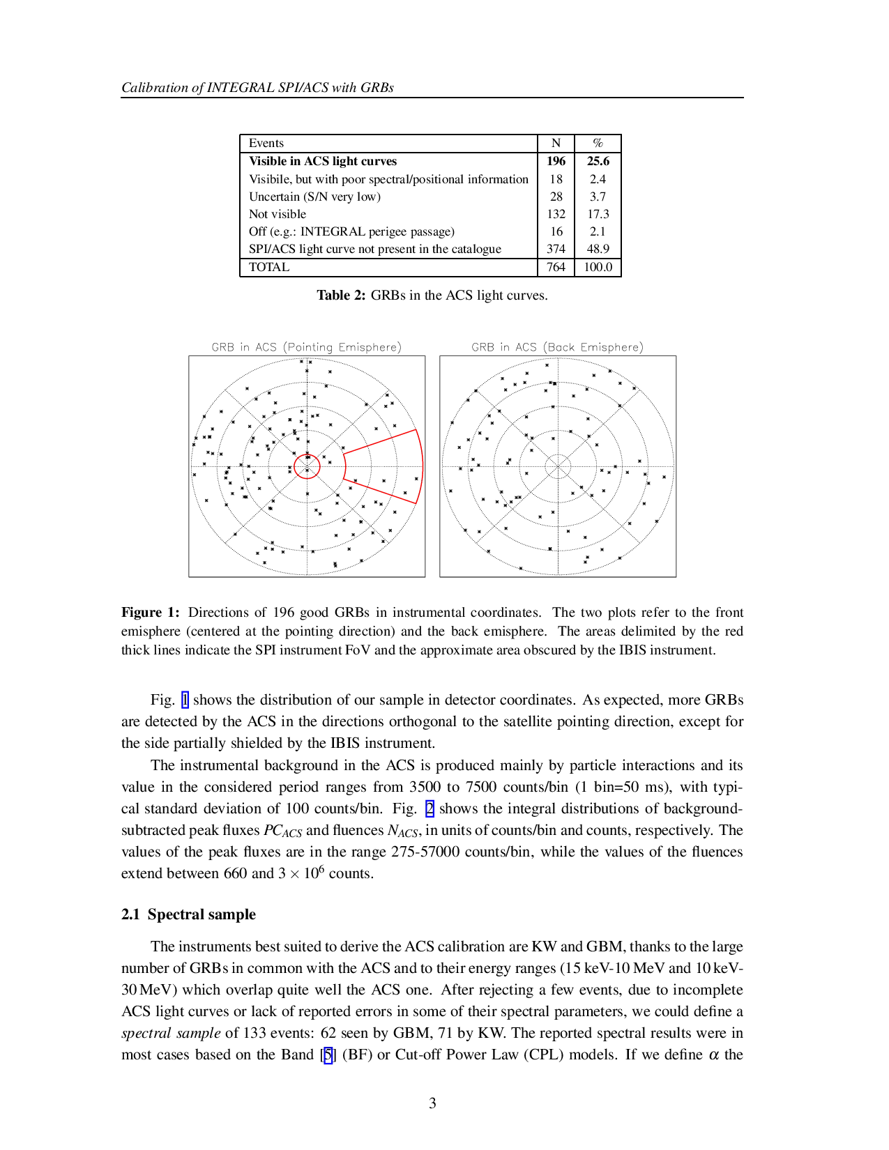
The Anti Coincidence Shield (ACS) of the INTEGRAL [1] SPI instrument [2] consists of 91 BGO crystals covering the lateral and bottom sides of the spectrometer [3]. The ACS provides veto signals for charged particles and gamma rays coming from outside the field of view (FoV). Its effective area, depending on energy and direction, has been computed for a set of directions and energies by means of Monte Carlo simulations [4], but no dedicated in-flight calibrations were performed. Using Gamma Ray Bursts (GRBs) it is possible to derive at least a rough in-flight calibration, i.e. a conversion factor from the instrument counting rate to physical flux units. This requires the knowledge of spectral and positional data of GRBs seen by at least another satellite besides the ACS.
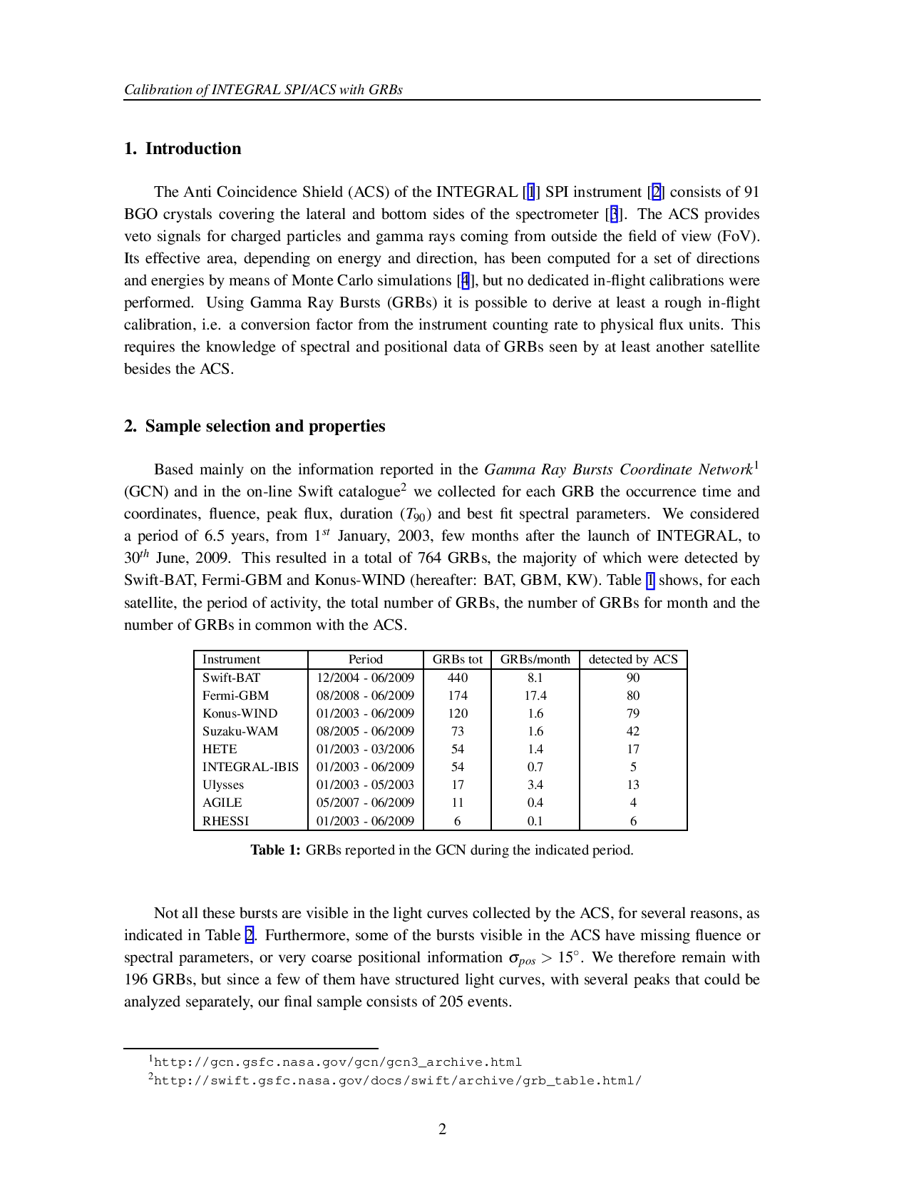
Based mainly on the information reported in the Gamma Ray Bursts Coordinate Network1 (GCN) and in the on-line Swift catalogue2 we collected for each GRB the occurrence time and coordinates, fluence, peak flux, duration (T 90 ) and best fit spectral parameters. We considered a period of 6.5 years, from 1 st January, 2003, few months after the launch of INTEGRAL, to 30 th June, 2009. This resulted in a total of 764 GRBs, the majority of which were detected by Swift-BAT, Fermi-GBM and Konus-WIND (hereafter: BAT, GBM, KW). Table 1 shows, for each satellite, the period of activity, the total number of GRBs, the number of GRBs for month and the number of GRBs in common with the ACS. Not all these bursts are visible in the light curves collected by the ACS, for several reasons, as indicated in Table 2. Furthermore, some of the bursts visible in the ACS have missing fluence or spectral parameters, or very coarse positional information σ pos > 15 • . We therefore remain with 196 GRBs, but since a few of them have structured light curves, with several peaks that could be analyzed separately, our final sample consists of 205 events. Fig. 1 shows the distribution of our sample in detector coordinates. As expected, more GRBs are detected by the ACS in the directions orthogonal to the satellite pointing direction, except for the side partially shielded by the IBIS instrument.
The instrumental background in the ACS is produced mainly by particle interactions and its value in the considered period ranges from 3500 to 7500 counts/bin (1 bin=50 ms), with typical standard deviation of 100 counts/bin. Fig. 2 shows the integral distributions of backgroundsubtracted peak fluxes PC ACS and fluences N ACS , in units of counts/bin and counts, respectively. The values of the peak fluxes are in the range 275-57000 counts/bin, while the values of the fluences extend between 660 and 3 × 10 6 counts.
The instruments best suited to derive the ACS calibration are KW and GBM, thanks to the large number of GRBs in common with the ACS and to their energy ranges (15 keV-10 MeV and 10 keV-30 MeV) which overlap quite well the ACS one. After rejecting a few events, due to incomplete ACS light curves or lack of reported errors in some of their spectral parameters, we could define a spectral sample of 133 events: 62 seen by GBM, 71 by KW. The reported spectral results were in most cases based on the Band [5] (BF) or Cut-off Power Law (CPL) models. If we define α the
We found that the ACS conversion factors derived using the peak fluxes have a wider dispersion than those derived using the fluences. This is due to the fact that peak fluxes have larger statistical errors and less constrained spectral parameters. Furthermore, the reported values often refer to different time integration intervals, thus introducing another source of uncertainty in the ACS comparison. We therefore based our analysis on the GRB fluences, computing for each burst the following quantity
where N ACS is the measured fluence in ACS counts and f ACS is the fluence in physical units obtained by converting the KW or GBM results to the ACS energy range. In this conversion we took into account the 90% c.l. errors on all the parameters in order to estimate the error on k. We defined the conversion factor as k, i.e. the weighted average of k. The conversion factor depends on the energy range used for f ACS . We have assumed E min =75 keV, and different values for E max as indicated in the first column of Table 3.
The large dispersion of k around the mean value (see Fig. 3 and values of χ2 in Table 3) can be ascribed to the directional and spectral variety of the sample. To investigate this effect, we divided our spectral sample in three subsamples: top zone events (θ < 45 • ), central zone events (45 • < θ < 120 • , excluding IBIS obscured zone), bottom zone events (θ > 120 • ), where θ is the angle from the pointing direction. However, the large dispersion of k values also for the three individual subsamples indicates that they also depend significantly on the spectral variety. Therefore, we studied the dependence of k on the GRB spectra, that we characterized by the hardness ratio defined as follows. We ch
…(Full text truncated)…
This content is AI-processed based on ArXiv data.