Optimal Scheduling for Fair Resource Allocation in Ad Hoc Networks with Elastic and Inelastic Traffic

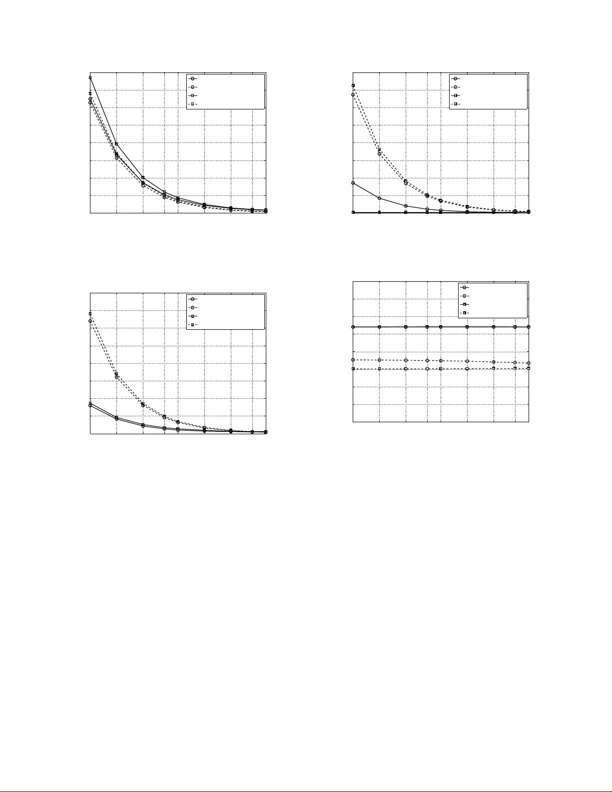
Optimal Scheduling for F air Resource Allocati on in Ad Hoc Netw orks with Elastic and Inelastic T raf fic Juan Jos ´ e Jaramillo Coordinated Science Labora tory and Departmen t of Electrical and Computer Engineer ing University of Illinois at Urban a-Champa ign Email: jjjarami@illinois.edu R. Srikant Coordinated Science Labora tory an d Departmen t of Elec trical and Computer Eng ineering University of Illinois at Ur bana-Cha mpaign Email: rsrikan t@illinois.edu Abstract —This paper stud ies the problem of congestion control and scheduling in ad hoc wireless networks that have to su pport a mixture of best-effort and real-time traffic. Optimization and stochastic network theory ha ve been succe ssful in designing ar chi- tectures f or fair resource allocation to meet long-term throughput demands. Howev er , to t he best of our knowledge, strict packet delay deadlines were not considered in this framew ork previously . In th is paper , we propose a model fo r incorporating th e quality of service (QoS) requirem ents of packets with deadlines in the optimization framework. The soluti on to the p roblem results in a join t congestion control and scheduling algorithm wh ich f airly allocates resource s to meet the fairness ob jectiv es of both elastic and inelastic flows, and per -packet delay requirem ents of inelastic flows. I . I N T RO D U C T I O N As wireless networks become mor e prev alent, they will b e expected to supp ort a wide variety of services, in cluding best- effort and real-time traffic. Such networks will hav e to serve flows that req uire q uality of service req uirements, such as minimum b andwidth a nd m aximum d elay co nstraints, wh ile at the same time keeping the network queues stable for data traffic a nd guaranteein g throu ghpu t op timality . For th e case of wireless networks with best-effort traffic only , op timization- based algorithms which naturally map into different layers of the proto col stack have been pro posed in the last few years [1]–[6 ]; see [ 7] for a survey . However , th ese mod els do not take into accoun t strict p er-packet delay b ounds. Scheduling packets with strict deadlines has been stud ied in [8]–[1 1], but all of these papers p rovide approximate solutions. The model that we study in this paper builds up on th e recent work in [ 12]–[ 14] on ad mission contr ol and sche duling for inelastic flows in collocated wireless n etworks, i.e., networks where all links interfere with e ach other . Amon g the many contributions in these papers is a k ey modeling innov ation whereby the n etwork is studied in frames, where a fr ame is a co ntiguou s set of tim e-slots o f fixed du ration. Packets with deadlines are assumed to arri ve at the beginning of a f rame and have to be served by th e end of the frame. In this p aper, we explore this modeling paradigm fur ther to st ud y the design of r esource allo cation algo rithms for ad hoc networks. The Researc h supported by NSF Grants 07-21286, 05-19691, 03-25673, ARO MURI Subcontracts, AFOSR Grant F A-9550-08-1-0432 and DTRA Grant HDTRA1-08-1-0016. frame-b ased model allows us to incor porate d elay deadlines in the optim ization framework for very g eneral n etwork models, and somewhat surp risingly , allows us to design a common framework for hand ling both elastic and inelastic flows. The main contr ibutions of the pap er are as follows: 1) W e present an o ptimization framework for resource allocation in a wireless n etwork co nsisting of both best- effort flows an d flows that genera te traffic with per- packet de lay constrain ts. Th e framework allows for very general interferen ce, cha nnel and arrival models. 2) Using a du al decompo sition app roach, we derive an optimal sched uling an d co ngestion contro l algorith m that fairly allocates resour ces and ensure s that a r equired fraction of each inelastic flo w’ s packets are deliv ered on time by appea ling to connections between Lagrang e multipliers, qu eues, and service deficits. The schedul- ing algorithm seamlessly integrates inelastic and elastic traffic into a unified m ax-weigh t sched uling framework, extending th e well-kn own results in [1 5]. 3) The conver gen ce of the above alg orithm in an approp ri- ate stoch astic sense is proved and it is also shown that the network is stable. I I . N E T W O R K M O D E L The network is represented by a dir ected graph G = ( N , L ) , where N is the set of nod es an d L is the set of directio nal links su ch that f or all n 1 , n 2 ∈ N if ( n 1 , n 2 ) ∈ L th en node n 1 can tr ansmit to no de n 2 . The link s are num bered 1 throug h |L| , and by abusing notatio n, we some times use l ∈ L to mean l ∈ { 1 , 2 , . . . , |L|} . T raffic is assumed to b e a m ixture o f elastic and inelastic flows, where an inelastic flo w is one th at h as maximum p er- packet delay requirements. In contrast, elastic flows d o no t have such requ irements. T ime is divided in slots, where a set of T consecutiv e time slots makes a frame . W e assume that packet arriv als only occur at the beginn ing of a fr ame, an d every inelastic packet has a deadline of T time slots. I f a pac ket misses its d eadline it is discarded, and it is r equired that the loss pr obability at link l ∈ L due to de adline expiry mu st be no more than p l . For elastic traffic we a ssociate a utility fu nction U l ( x l ) which is 2 a function of the mean elastic arrival rate per frame x l . W e assume that U l ( . ) is a co ncave function . For a giv en frame, we deno te b y the vector a i = ( a il ) l ∈L the n umber of inelastic packet a rriv als at every link, wh ere a il is a rando m variable with mean λ l and variance σ 2 il . W e further assume that arri vals ar e indep endent b etween different frames and that P r ( a il = 0) > 0 an d P r ( a il = 1) > 0 . The last two assumptions ar e used to guar antee that the Markov chain we define later is both irredu cible and ap eriodic, althou gh th ese can be r eplaced by oth er similar assumption s. Similarly , we define a e = ( a el ) l ∈L to be the n umber of elastic packet arri vals at every link in a gi ven frame. The ch annel state is assumed to be co nstant in a g iv en frame, indep endent between different fram es, an d in depend ent of arri vals. The vector c = ( c l ) l ∈L denotes the num ber of packets lin k l ca n successfully tran smit on a time slot in a giv en frame. Dependin g on th e wireless tech nolog y used, we can have some channel feedba ck before or after a transmission oc curs. If ch annel estimation is per formed before transmitting, we can determine the optimal rate at which we can successfully transmit. Alterna ti vely , f eedback fro m the recei ver after the transmission c an be used to detect if a transmission is suc- cessful o r n ot. In this paper we tr y to captur e both scenarios in the following cases: 1) Known chann el state: It is assumed that c l is a non - ne gative rando m variable with mean ¯ c l and variance σ 2 cl , and we get to know the channel state at th e be ginn ing of the fra me. 2) Unknown channel state: It is assumed that c l is a Bernoulli ran dom variable with mean ¯ c l and we only get to know the channel state at th e end of the frame. In the kn own chan nel state case where we do c hannel estimation to determine the optimal transmission r ate, we can po tentially sen d mo re than one p acket in a time slot at higher rates. This is captu red by t he fact that we m ake no assumptio ns on th e values c l can take since it will b e determined by the par ticular wireless technolog y used . In the case of un known channel state we assume that we only ge t the binary feedback o f ack nowledgments, which is reflected in th e Bernoulli assumptio n o n c l . In this case, an d without any loss of generality , we assume only one packet can be transmitted per time slot p er link. In th e re st o f th e pap er we will consider the kn own cha nnel case first and th en in Section VI we will h ighlight the differences in the analysis for the un known chann el case. I I I . P R O BL E M F O R M U L A T I O N W e first fo rmulate the proble m as a static optim ization problem . Using deco mposition theo ry , we will the n obtain a dynamic solu tion to this p roblem an d prove its stability using stochastic L yap unov tech niques. A fea sible sche dule s = ( s il,t , s el,t ) is such that s il,t , s el,t respectively denote the number of in elastic and elastic packets that can be scheduled for transmission at link l ∈ L and time slot t ∈ { 1 , 2 , . . . , T } ; thus, s il,t + s el,t > 0 means that link l is scheduled to tr ansmit in time slot t of the fra me. Fu rthermo re, for any t , if s il 1 ,t + s el 1 ,t > 0 and s il 2 ,t + s el 2 ,t > 0 then links l 1 and l 2 can be scheduled to simultaneously transmit without interfering with each oth er . Assuming the inelastic arrivals and the chan nel state are given by a i and c respec ti vely , we ha ve the following co nstraints: T X t =1 s il,t ≤ a il for all l ∈ L and (1) s il,t + s el,t ≤ c l for all l ∈ L and t ∈ { 1 , 2 , . . . , T } . (2) W e den ote by S ( a i , c ) the set of all feasible sched ules when the a rriv al state is a i and the chann el state is c ; thus, S ( a i , c ) captures any interfer ence con straints w e hav e on our n etwork and satisfies (1) an d (2). At the beginning of any frame we must choose a feasible schedule to serve all links and decide how ma ny elastic packets are allowed to be in jected in the network. Th erefor e, o ur goal is to find a f unction P r ( s | a i , c ) wh ich is the probab ility of using s ched ule s ∈ S ( a i , c ) wh en th e inelastic arrivals are giv en by a i and the channel state is c , subject to th e constrain t that the lo ss probab ility at link l ∈ L d ue to d eadline expiry cannot e xceed p l . For elastic traffic, we w ant to select the vector a e such th at we maximize th e ne twork utility wh ile keeping the queues stable. T o prope rly formu late the pro blem, let us first d efine µ i ( a i , c ) to b e the expected number of inelastic p ackets served if the number of packet ar riv als is given by a i and the channel state is c . Similarly , µ e ( a i , c ) d enotes the expe cted number of elastic pa ckets that can b e ser ved. There fore, we have the following co nstraints: µ il ( a i , c ) ≤ X s ∈S ( a i ,c ) T X t =1 s il,t P r ( s | a i , c ) µ el ( a i , c ) ≤ X s ∈S ( a i ,c ) T X t =1 s el,t P r ( s | a i , c ) . The expected service for mixed tr affic at lin k l is then g iv en by µ il def = X a i X c µ il ( a i , c ) P r ( c ) P r ( a i ) µ el def = X a i X c µ el ( a i , c ) P r ( c ) P r ( a i ) and due to QoS re quiremen ts a nd capacity con straints, we require that µ il ≥ λ l (1 − p l ) and x l ≤ µ el . W e will f ocus o n max imizing the following o bjective for some given vector w ∈ R |L| + : max µ i ( a i ,c ) ,µ e ( a i ,c ) , µ i ,µ e ,x,P r ( s | a i ,c ) X l ∈L U l ( x l ) + w l µ il (3) 3 subject to µ il ( a i , c ) ≤ X s T X t =1 s il,t P r ( s | a i , c ) fo r a ll l ∈ L , a i , c µ el ( a i , c ) ≤ X s T X t =1 s el,t P r ( s | a i , c ) fo r a ll l ∈ L , a i , c µ il = X a i X c µ il ( a i , c ) P r ( c ) P r ( a i ) fo r all l ∈ L µ el = X a i X c µ el ( a i , c ) P r ( c ) P r ( a i ) fo r all l ∈ L µ il ≥ λ l (1 − p l ) for all l ∈ L 0 ≤ x l ≤ µ el for all l ∈ L P r ( s | a i , c ) ≥ 0 for all s ∈ S ( a i , c ) , a i , c X s P r ( s | a i , c ) ≤ 1 f or all a i , c. The vector w can be used to allocate additional bandwidth fairly to inelastic flows beyon d what is required to meet their Qo S needs. Other uses for w w ill b e e xplo red in the simulations section. W e will assume that th e ar riv als and loss probab ility requireme nts are feasible and thus the op timization problem has a solution ( x ∗ , µ ∗ i ) . I V . S O L U T IO N U S I N G D UA L D E C O M P O S I T I O N Using the definition of th e dual function [16], we ha ve that D ( δ i , δ e ) = max µ i ( a i ,c ) ,µ e ( a i ,c ) , µ i ,µ e ,x,P r ( s | a i ,c ) X l ∈L  U l ( x l ) + w l µ il − δ el [ x l − µ el ] − δ il [ λ l (1 − p l ) − µ il ]  subject to µ il ( a i , c ) ≤ X s T X t =1 s il,t P r ( s | a i , c ) fo r a ll l ∈ L , a i , c µ el ( a i , c ) ≤ X s T X t =1 s el,t P r ( s | a i , c ) fo r a ll l ∈ L , a i , c µ il = X a i X c µ il ( a i , c ) P r ( c ) P r ( a i ) fo r all l ∈ L µ el = X a i X c µ el ( a i , c ) P r ( c ) P r ( a i ) fo r all l ∈ L x l ≥ 0 fo r all l ∈ L P r ( s | a i , c ) ≥ 0 for all s ∈ S ( a i , c ) , a i , c X s P r ( s | a i , c ) ≤ 1 f or all a i , c. Slater’ s co ndition [ 17] states that, since th e objective is concave and th e c onstraints ar e affi ne function s, the duality gap is zero and theref ore D ( δ ∗ i , δ ∗ e ) = P l ∈L U l ( x ∗ l ) + w l µ ∗ il , where ( δ ∗ i , δ ∗ e ) ∈ arg min δ il ≥ 0 ,δ el ≥ 0 D ( δ i , δ e ) . W e ar e in terested in finding ( x ∗ , µ ∗ i ) but not the value D ( δ ∗ i , δ ∗ e ) , so if we rewrite the objective in the d ual fun ction as max µ i ( a i ,c ) ,µ e ( a i ,c ) , µ i ,µ e ,x,P r ( s | a i ,c )          P l ∈L U l ( x l ) − δ el x l + P l ∈L ( w l + δ il ) µ il + δ el µ el − P l ∈L δ il λ l (1 − p l )          we notice that the pro blem can be decomposed into the following sub problem s: max x l ≥ 0 U l ( x l ) − δ el x l and max µ i ( a i ,c ) ,µ e ( a i ,c ) , µ i ,µ e ,P r ( s | a i ,c ) X l ∈L ( w l + δ il ) µ il + δ el µ el (4) subject to µ il ( a i , c ) ≤ X s T X t =1 s il,t P r ( s | a i , c ) for all l ∈ L , a i , c µ el ( a i , c ) ≤ X s T X t =1 s el,t P r ( s | a i , c ) for all l ∈ L , a i , c µ il = X a i X c µ il ( a i , c ) P r ( c ) P r ( a i ) for all l ∈ L µ el = X a i X c µ el ( a i , c ) P r ( c ) P r ( a i ) for all l ∈ L P r ( s | a i , c ) ≥ 0 f or all s ∈ S ( a i , c ) , a i , c X s P r ( s | a i , c ) ≤ 1 for all a i , c. Furthermo re, since we ar e interested in solvin g th e proble m for non-negativ e values of δ il and δ el , it m ust be the case that µ ∗ i and µ ∗ e are as large as the constraints allow , and since the upper bounds fo r µ ∗ il ( a i , c ) an d µ ∗ el ( a i , c ) are expressed as a conve x comb ination, an d th e objecti ve fu nction in (4) is linear, th e problem can be decompo sed in to the following subprob lems for fixed a i and c : max s ∈S ( a i ,c ) X l ∈L ( ( w l + δ il ) T X t =1 s il,t + δ el T X t =1 s el,t ) . This sug gests the f ollowing iterative alg orithm to find the solution to our optim ization problem, where k is the step index and X max > max l ∈L x ∗ l is a fixed parameter : ˜ x ∗ l ( k ) ∈ arg ma x 0 ≤ x l ≤ X max U l ( x l ) − δ el ( k ) x l 4 ˜ s ∗ ( a i , c, k ) ∈ arg max s ∈S ( a i ,c ) X l ∈L ( [ w l + δ il ( k )] T X t =1 s il,t + δ el ( k ) T X t =1 s el,t ) ˜ µ ∗ il ( k ) = X a i X c T X t =1 ˜ s ∗ il,t ( a i , c, k ) P r ( c ) P r ( a i ) ˜ µ ∗ el ( k ) = X a i X c T X t =1 ˜ s ∗ el,t ( a i , c, k ) P r ( c ) P r ( a i ) . W e update the Lagran ge multipliers δ i ( k ) , δ e ( k ) at every step accordin g to th e following equ ations: δ il ( k + 1) = { δ il ( k ) + ǫ [ λ l (1 − p l ) − ˜ µ ∗ il ( k )] } + and δ el ( k + 1 ) = { δ el ( k ) + ǫ [ ˜ x ∗ l ( k ) − ˜ µ ∗ el ( k )] } + where ǫ > 0 is a fixed step-size p arameter, and fo r any α ∈ R , α + def = max { α, 0 } . Making the chan ge of variables ǫ ˆ d ( k ) = δ i ( k ) and ǫ ˆ q ( k ) = δ e ( k ) , we hav e that o ur iter ativ e algorithm can be rewritten as ˜ x ∗ l ( k ) ∈ arg ma x 0 ≤ x l ≤ X max 1 ǫ U l ( x l ) − ˆ q l ( k ) x l ˜ s ∗ ( a i , c, k ) ∈ arg max s ∈S ( a i ,c ) X l ∈L ( [ 1 ǫ w l + ˆ d l ( k )] T X t =1 s il,t + ˆ q l ( k ) T X t =1 s el,t ) ˜ µ ∗ il ( k ) = X a i X c T X t =1 ˜ s ∗ il,t ( a i , c, k ) P r ( c ) P r ( a i ) ˜ µ ∗ el ( k ) = X a i X c T X t =1 ˜ s ∗ el,t ( a i , c, k ) P r ( c ) P r ( a i ) . with upd ate eq uations ˆ d l ( k + 1 ) = [ ˆ d l ( k ) + λ l (1 − p l ) − ˜ µ ∗ il ( k )] + ˆ q l ( k + 1) = [ ˆ q l ( k ) + ˜ x ∗ l ( k ) − ˜ µ ∗ el ( k )] + . It should be noted that due to the ch ange of variables ˆ d l ( k ) can be interpre ted as a q ueue that has λ l (1 − p l ) arriv als and ˜ µ ∗ il ( k ) departu res at step k ; ˆ q l ( k ) can have a similar qu eue interpretatio n. The dual decomposition approach only provides an intu ition beh ind the solution, but the real network h as stochastic a nd dynamic ar riv als an d channel state cond itions. In the next section, we present the com plete so lution which takes into accou nt these dynamic s a nd we also establish its conv ergence pr operties. V . D Y NA M I C A L G O R I T H M A N D I T S C O N V E R G E N C E A N A L Y S I S A. Scheduler and Congestion Contr o ller T o implement the algorithm online, we p ropo se the follow- ing con gestion control algo rithm in f rame k , where the queue length at link l is given by q l ( k ) : ˜ x ∗ l ( k ) ∈ arg ma x 0 ≤ x l ≤ X max 1 ǫ U l ( x l ) − q l ( k ) x l . (5) W e need to co n vert this elastic arr iv al rate, which in gener al is a no n-negative re al n umber, into a non-n egativ e integer indicating the number o f elastic packets allowed to enter th e network in a g iv en frame. This con version can be made in many different ways: we assume the e lastic arr i vals at link l , ˜ a el ( k ) , are a random variable with mean ˜ x ∗ l ( k ) and variance upper-boun ded by σ 2 e , an d are such that P r (˜ a el ( k ) = 0) > 0 and P r (˜ a el ( k ) = 1) > 0 for all l ∈ L and all k . The last two assumptio ns ar e u sed to gu arantee the Markov chain we define b elow is both irredu cible and aper iodic, althou gh these can be replaced by o ther similar assumption s. Letting the number of inelastic arrivals be d enoted by a i ( k ) and the channel state by c ( k ) , we prop ose the fo llowing scheduling algor ithm: ˜ s ∗ ( a i ( k ) , c ( k ) , d ( k ) , q ( k )) ∈ (6) arg max s ∈S ( a i ( k ) ,c ( k )) X l ∈L ( [ 1 ǫ w l + d l ( k )] T X t =1 s il,t + q l ( k ) T X t =1 s el,t ) . The vectors d ( k ) and q ( k ) ar e up dated from fr ame to fr ame as follows: d l ( k + 1) = [ d l ( k ) + ˜ a il ( k ) − I ∗ il ( a i ( k ) , c ( k ) , d ( k ) , q ( k ))] + q l ( k + 1 ) = [ q l ( k ) + ˜ a el ( k ) − I ∗ el ( a i ( k ) , c ( k ) , d ( k ) , q ( k ))] + , where I ∗ il ( a i ( k ) , c ( k ) , d ( k ) , q ( k )) = T X t =1 ˜ s ∗ il,t ( a i ( k ) , c ( k ) , d ( k ) , q ( k )) I ∗ el ( a i ( k ) , c ( k ) , d ( k ) , q ( k )) = T X t =1 ˜ s ∗ el,t ( a i ( k ) , c ( k ) , d ( k ) , q ( k )) and ˜ a il ( k ) is a binom ial rand om variable with parameter s a il ( k ) a nd 1 − p l . T he q uantity ˜ a il ( k ) can b e gen erated by the n etwork as f ollows: upon e ach in elastic packet arrival, toss a coin with pro bability o f heads eq ual to 1 − p l , and if the outcome is head s , add a one to the deficit c ounter . In our notation we make explicit th e fact that f or fixed ǫ and w , the optimal sche duler (6) is a functio n of a i ( k ) , c ( k ) , d ( k ) , and q ( k ) . W e interpret d l ( k ) as a virtual q ueue that counts the deficit in serv ice for link l to achieve a loss pro bability due to deadline expir y less tha n o r eq ual to p l . Th is d eficit qu eue was first used in the inelastic traffic context in [12] for the case of collocated n etworks; th e con nection to th e du al de composition approa ch n ow provid es a Lag range multip lier interpr etation to it and allows the extension to general ad h oc network s. Note that q l ( k ) is ju st the queue size f or elastic packets at link l . 5 B. Conver gence Results For readability , we pre sent the main results in this section, but th e proofs are defer red t o the append ixes. W e start by noting tha t ( d ( k ) , q ( k )) defines an irred ucible and aperio dic Markov ch ain. T o prove that our d ynamic algorithm achieves the optimal solution to th e static pro blem (3 ) in some average sense and fulfills all links’ req uirements, we will first boun d the expected drift of ( d ( k ) , q ( k )) fo r a suitable L yap unov function . Lemma 1: Consider th e L y apunov functio n V ( d, q ) = 1 2 P l ∈L d 2 l + q 2 l . If µ ∗ il > λ l (1 − p l ) and µ ∗ el > x ∗ l for all l ∈ L , then E [ V ( d ( k + 1) , q ( k + 1)) | d ( k ) = d, q ( k ) = q ] − V ( d, q ) ≤ B 1 − B 2 X l ∈L d l − B 3 X l ∈L q l − 1 ǫ X l ∈L [ U l ( x ∗ l ) − U l ( ˜ x ∗ l ( k ))] − 1 ǫ X l ∈L w l µ ∗ il − w l E [ I ∗ il ( a i ( k ) , c ( k ) , d, q )] for some positive co nstants B 1 , B 2 , B 3 , a ny ǫ > 0 , wher e ( x ∗ , µ ∗ i ) is the solution to (3), ˜ x ∗ ( k ) is the solution to (5), and I ∗ i ( a i ( k ) , c ( k ) , d, q ) is ob tained f rom the solution to (6). ⋄ It is important to no te that since the last two te rms in the right-han d side of the in equality can be up per-bounded , Lemma 1 im plies tha t ( d ( k ) , q ( k )) is p ositi ve recurr ent since the expected drift is negati ve but f or a fin ite set o f values of ( d ( k ) , q ( k )) . As a direct co nsequen ce of this fact, we note that the to tal service deficit and queue leng th ha ve a O (1 / ǫ ) bound . Cor o llary 1: If µ ∗ il > λ l (1 − p l ) and µ ∗ el > x ∗ l for all l ∈ L , then the total expected service deficit and n etwork queue length is upp er-bounded by lim s up k →∞ E " X l ∈L d l ( k ) + q l ( k ) # ≤ B 4 + 1 ǫ B 5 for all l ∈ L and B 4 = B 1 min { B 2 , B 3 } and B 5 ≤ P l ∈L max 0 ≤ x l ≤ X max 2 | U l ( x l ) | + w l λ l min { B 2 , B 3 } . ⋄ This also implies that th e sched uling an d con gestion con trol algorithm fulfills all link s’ inelastic requir ements. Cor o llary 2: If µ ∗ il > λ l (1 − p l ) and µ ∗ el > x ∗ l for all l ∈ L , then the on line algorithm fulfills all the inelastic co nstraints. That is: lim inf K → ∞ E " 1 K K X k =1 I ∗ il ( a i ( k ) , c ( k ) , d ( k ) , q ( k )) # ≥ λ l (1 − p l ) for all l ∈ L . ⋄ The above corollar y simply states that the arriv al rate into the d eficit co unter is less than or eq ual to the departur e rate. This r esult is an obviou s consequence of the stability of the deficit counters and so a f ormal pro of is not provided here. Now we are rea dy to prove that our on line algo rithm is within O ( ǫ ) of the op timal v alue. Theor em 1: For any ǫ > 0 , if µ ∗ il > λ l (1 − p l ) and µ ∗ el > x ∗ l for all l ∈ L , then lim s up K → ∞ E " X l ∈L U l ( x ∗ l ) + w l µ ∗ il − X l ∈L 1 K K X k =1 U l ( ˜ x ∗ l ( k )) − X l ∈L 1 K K X k =1 w l I ∗ il ( a i ( k ) , c ( k ) , d ( k ) , q ( k )) # ≤ B ǫ for some B > 0 , where ( x ∗ , µ ∗ i ) is the solution to ( 3), ˜ x ∗ ( k ) is the so lution to (5), an d I ∗ i ( a i ( k ) , c ( k ) , d ( k ) , q ( k )) is ob tained from the solution to ( 6). ⋄ In con clusion, th ere is a trade-o ff in choo sing th e param eter ǫ : smaller values will achiev e a solution closer to the optimal, but at th e sam e time the d eficit in service at the links and the aggregate queu e length increase. The statement and th e p roof of Theorem 1 fo llows th e techniqu es in [3]. The result can also be d erived, in a slightly different fo rm, u sing th e tech niques in [4]. A c losely r elated result can be obtain ed using the metho ds in [1]. V I . U N K N O W N C H A N N E L S TA T E The a nalysis for the unknown channel case is similar to the one we presen ted for the known channel case, so in this section we will on ly highligh t the differences. A feasible schedu le s = ( s il,t , s el,t ) is such that s il,t , s el,t respectively denote the num ber o f inelastic and elastic packets that can be sched uled for tran smission at link l ∈ L and time t ∈ { 1 , 2 , . . . , T } without v iolating any inter ference constraints. Assuming the inelastic ar riv als ar e g iv en by a i , and since we can on ly schedule at most one packet per link at every time slot, we h av e the f ollowing constraints: T X t =1 s il,t ≤ a il for all l ∈ L and (7) s il,t + s el,t ≤ 1 for all l ∈ L an d t ∈ { 1 , 2 , . . . , T } . (8) W e denote by S ( a i ) the set of all feasible schedu les for fixed arriv als, captu ring any in terferenc e con straints we hav e on our network, and satisfying (7) an d ( 8). Our goal now is to find a function P r ( s | a i ) which is the probab ility of using sch edule s ∈ S ( a i ) when t he in elastic arriv als are given b y a i , sub ject to th e co nstraint th at the loss probab ility at link l ∈ L due to deadline expiry canno t exceed p l . For elastic traffic, we still want to select th e vector a e such that we maximize the total utility while keepin g the queu es stable. For a given d istribution P r ( s | a i ) we h av e that µ il ( a i ) is the expected numb er of attem pted inelastic tran smissions if arriv als a re giv en by a i . Similarly , µ el ( a i ) den otes the expected 6 number of times link l is scheduled to serve elastic packets in a given frame. As b efore, we have the f ollowing con straints: µ il ( a i ) ≤ X s T X t =1 s il,t P r ( s | a i ) µ el ( a i ) ≤ X s T X t =1 s el,t P r ( s | a i ) When the (unk nown) channe l state is c , we have that c l µ il ( a i ) is the expected n umber of su ccessful inelastic trans- missions p er fram e at link l for fixed arriv als, while c l µ el ( a i ) is the expected service to link l for inelastic arr iv als. Th us, the expected service for mixed traffi c a t link l is given by µ il def = X a i X c c l µ il ( a i ) P r ( c ) P r ( a i ) µ el def = X a i X c c l µ el ( a i ) P r ( c ) P r ( a i ) . Simplifying both expre ssions we get µ il = X a i ¯ c l µ il ( a i ) P r ( a i ) µ el = X a i ¯ c l µ el ( a i ) P r ( a i ) . Due to service requirements and capacity co nstraints we need that µ il ≥ λ l (1 − p l ) and x l ≤ µ el . W ith the definitio ns and constraints stated above we can formu late the o ptimization problem in a similar way as in ( 3). The on ly difference with the known channel state case is the scheduling algorith m. Assuming inelastic arriv als a re given by a i ( k ) the schedu ling algorithm is given by ˜ s ∗ ( a i ( k ) , d ( k ) , q ( k )) ∈ arg max s ∈S ( a i ( k )) X l ∈L ( [ 1 ǫ w l + d l ( k )] ¯ c l T X t =1 s il,t + q l ( k ) ¯ c l T X t =1 s el,t ) . The main difference in the schedulin g algorithm compared to the known chann el state case is that the network now uses the expected ch annel state in making schedu ling decisions. Thus, the network need s to know or estimate ¯ c l as in [12 ]. Similar r esults can b e proved for th is a lgorithm using the technique s de veloped in Section V -B, where by one can show that the algor ithm mee ts all the inelastic QoS constraints, the total expected service d eficits an d the qu eue lengths hav e a O (1 / ǫ ) b ound , an d the mean value of the objective is w ithin O ( ǫ ) of the op timal value. 10 8 9 7 4 5 6 1 3 2 Fig. 1. Interfere nce graph used in the simulations V I I . S I M U L AT I ON S The p urpo se of this simulation study is to under stand how the par ameter ǫ and the lin k weights w l impact the perfor mance of the a lgorithm, and how a greedy heuristic can be used to implement the optim al schedu ler . W e simu late a 10-link network with an interfere nce gra ph giv en by Fig. 1, where each nod e repr esents a link and ea ch edge means that the two adjacent links cannot be scheduled simultaneou sly . F or example, if link 1 is scheduled, then links 2, 4, and 7 cannot be activ ated. The requ ired loss prob ability due to deadline expiry of inelastic packets is set to 0.1, th e link arriv als are assumed to have a Bernoulli distribution with me an 0.6 p ackets/frame, and there are 3 time slots per frame. The channel for e very link is a ssumed to have a Bernoulli distribution with mean 0.96 , and we get to know the channel state at the beginning of the frame. W e set U l ( x l ) = log ( x l ) for all links. The simu lation time was 10 6 frames. As can be noted from (6), the max-weight sched uler requires that we do an exhaustive search to find the optim al schedule at ev ery frame. For large networks this can bec ome a burden due to th e large search space; thus we explore a greedy h euristic and che ck h ow close it is to the o ptimal solution: at any given time slot, the g reedy scheduler ord ers all links acco rding to their weigh ts. The greedy sch eduler adds o ne o f the lin ks with the la rgest weight to the sched ule, then removes all lin ks th at interfere with th is link fr om the graph , then schedules a link with the largest weight among the remaining links, and so on. This procedure continues until no more links can be scheduled. In Figs. 2, 3 , and 4, we plot the expected values of the deficit counters and q ueues per link f or various values of w l , and compare their evolution for bo th th e sched uler with optimal decisions and the gree dy scheduler . W e see that as w l increases, the deficit co unters bec ome small. The upper boun d in Coro llary 1 only suggests that the sum o f the deficit counter s and queues is O (1 /ǫ ) . T hus, it is interesting to note that by changin g w l , on e can nearly eliminate the b acklog in deficit f or in elastic traffic while maintaining the same order o f queue sizes. The reason for this can be un derstood by examin ing the schedu ling algorith m (6). Note that the alg orithm gi ves priority to elastic traffic if queues ar e larger than counters. When w l is small co mpared to ǫ , th e effect o f w l is negligible in the scheduling alg orithm. On the o ther hand , when w l is O (1) , w l /ǫ is O (1 / ǫ ) which is co mparab le to the queu e leng ths an d hence , the deficit does not have to be large to provid e service to inelastic tr affic under algorithm (6). 7 0.01 0.02 0.04 0.07 0.1 0.2 0.4 0.7 1 0 50 100 150 200 250 300 350 400 ε Deficit and Queue Size Ave. deficit (optimal) Ave. queue (optimal) Ave. deficit (greedy) Ave. queue (greedy) Fig. 2. Deficit size and queue length when w l = 0 0.01 0.02 0.04 0.07 0.1 0.2 0.4 0.7 1 0 50 100 150 200 250 300 350 400 ε Deficit and Queue Size Ave. deficit (optimal) Ave. queue (optimal) Ave. deficit (greedy) Ave. queue (greedy) Fig. 3. Deficit size and queue length when w l = 3 It m ust be noted that small deficit counters mea n that th ere is a small backlog in p roviding acceptable serv ice to inelastic arriv als. For the case of real-time traf fic this is a desirable proper ty , since we d o n ot want to ha ve large variations in th e service pr ovided that could affect the p erceived quality . Th us, ev en if f air allocation of bandwidth beyond the minimum is not required for inelastic flo ws, choo sing w l an order of magnitud e larger th an ǫ is desirab le to maintain small deficits. As can be noted , the greed y sched uler seems to giv e lower deficit values than the optimal sched uler for larger values of w l . W e believe that the reason is th at weights given to inelastic flows increa se with increasing w l and therefor e, the g reedy scheduler picks them first. Howev er, o ur o ptimality goal is giv en by (3) wh ich is determined by th e rates receiv ed by the various flows. The rates achieved by th e two schedulers are quite close in the simu lations, as seen in Figs. 5, 6, and 7, while keeping the dr oppin g pro babilities below the requiremen t, as shown in Figs. 8, 9, and 10. 0.01 0.02 0.04 0.07 0.1 0.2 0.4 0.7 1 0 50 100 150 200 250 300 350 400 ε Deficit and Queue Size Ave. deficit (optimal) Ave. queue (optimal) Ave. deficit (greedy) Ave. queue (greedy) Fig. 4. Deficit size and queue length when w l = 6 0.01 0.02 0.04 0.07 0.1 0.2 0.4 0.7 1 0 0.1 0.2 0.3 0.4 0.5 0.6 0.7 0.8 ε Average Service for Traffic Inelastic (optimal) Elastic (optimal) Inelastic (greedy) Elastic (greedy) Fig. 5. A verage service when w l = 0 V I I I . C O N C L U S I O N S In this pape r we ha ve presented an optim ization framework for the pro blem of congestion contro l and scheduling of elastic and inela stic tr affic in ad ho c wire less n etworks. The model was developed for gener al interfere nce graphs, gen eral arrivals and ti me- varying channels. Usi ng a du al function appro ach we presented a dec omposition of the pro blem into an online algorithm that is ab le to make optima l decisions while keeping the network stable and fu lfilling the inelastic flow’ s QoS constraints. A k ey result is that, through the u se of d eficit counters, on e can treat the sched uling problem fo r elastic an d inelastic flo ws in a com mon framework. It is also inter esting to note tha t the de ficit cou nters introdu ced in [12]– [14] hav e the interpretatio n of Lagrange multipliers. Simulations corrob orate our results and show the d epende ncy of the pe rforman ce of the algorithm on the aux iliary p arameter ǫ an d its ro le in to assigning resources to both elastic and inelastic traffic. W e note that, in the unknown channel case, we do not consider channel feedbac k at the en d of each time slot as in [12] –[14] . This will be add ressed in future work. 8 0.01 0.02 0.04 0.07 0.1 0.2 0.4 0.7 1 0 0.1 0.2 0.3 0.4 0.5 0.6 0.7 0.8 ε Average Service for Traffic Inelastic (optimal) Elastic (optimal) Inelastic (greedy) Elastic (greedy) Fig. 6. A verage service when w l = 3 0.01 0.02 0.04 0.07 0.1 0.2 0.4 0.7 1 0 0.1 0.2 0.3 0.4 0.5 0.6 0.7 0.8 ε Average Service for Traffic Inelastic (optimal) Elastic (optimal) Inelastic (greedy) Elastic (greedy) Fig. 7. A verage service when w l = 6 A P P E N D I X A P R O OF O F L E M M A 1 T o prove Lem ma 1, we start by first provin g two aux iliary lemmas and then stating a fact. Lemma 2: Given that at frame k we h av e the event d ( k ) = d and q ( k ) = q , then E " 1 2 X l ∈L { [ d l + ˜ a il ( k ) − I ∗ il ( a i ( k ) , c ( k ) , d, q )] + } 2 # − X l ∈L d 2 l 2 ≤ B 6 + X l ∈L d l λ l (1 − p l ) − E " X l ∈L  1 ǫ w l + d l  I ∗ il ( a i ( k ) , c ( k ) , d, q ) − X l ∈L 1 ǫ w l I ∗ il ( a i ( k ) , c ( k ) , d, q ) # for some non-negative constant B 6 , and where 0.01 0.02 0.04 0.07 0.1 0.2 0.4 0.7 1 0.065 0.070 0.075 0.080 0.085 0.090 0.095 0.100 0.105 ε Dropping Probability Optimal Greedy Fig. 8. Dropping probabilit y when w l = 0 0.01 0.02 0.04 0.07 0.1 0.2 0.4 0.7 1 0.065 0.070 0.075 0.080 0.085 0.090 0.095 0.100 0.105 ε Dropping Probability Optimal Greedy Fig. 9. Dropping probabilit y when w l = 3 I ∗ il ( a i ( k ) , c ( k ) , d, q ) is given by the solution to (6). ⋄ Pr o of: E " 1 2 X l ∈L { [ d l + ˜ a il ( k ) − I ∗ il ( a i ( k ) , c ( k ) , d, q )] + } 2 # − X l ∈L d 2 l 2 ≤ E " 1 2 X l ∈L [ d l + ˜ a il ( k ) − I ∗ il ( a i ( k ) , c ( k ) , d, q )] 2 # − X l ∈L d 2 l 2 = E " X l ∈L d l [˜ a il ( k ) − I ∗ il ( a i ( k ) , c ( k ) , d, q )] + 1 2 X l ∈L [˜ a il ( k ) − I ∗ il ( a i ( k ) , c ( k ) , d, q )] 2 # ≤ E " X l ∈L d l ˜ a il ( k ) − d l I ∗ il ( a i ( k ) , c ( k ) , d, q ) + 1 2 X l ∈L ˜ a 2 il ( k ) + a 2 il ( k ) # (9) 9 0.01 0.02 0.04 0.07 0.1 0.2 0.4 0.7 1 0.065 0.070 0.075 0.080 0.085 0.090 0.095 0.100 0.105 ε Dropping Probability Optimal Greedy Fig. 10. Dropping probabilit y when w l = 6 ≤ B 6 + X l ∈L d l λ l (1 − p l ) − E " X l ∈L  1 ǫ w l + d l  I ∗ il ( a i ( k ) , c ( k ) , d, q ) − X l ∈L 1 ǫ w l I ∗ il ( a i ( k ) , c ( k ) , d, q ) # where (9) follows fr om the definition of I ∗ il ( a i ( k ) , c ( k ) , d, q ) and B 6 = 1 2 X l ∈L ( λ 2 l + σ 2 il )[1 + (1 − p l ) 2 ] + λ l p l (1 − p l ) . Lemma 3: Given that at frame k we h av e the event d ( k ) = d and q ( k ) = q , then E " 1 2 X l ∈L { [ q l + ˜ a el ( k ) − I ∗ el ( a i ( k ) , c ( k ) , d, q )] + } 2 # − X l ∈L q 2 l 2 ≤ B 7 − 1 ǫ X l ∈L [ U l ( x ∗ l ) − U l ( ˜ x ∗ l ( k ))] − X l ∈L q l { E [ I ∗ el ( a i ( k ) , c ( k ) , d, q )] − x ∗ l } for som e con stant B 7 > 0 , whe re x ∗ and ˜ x ∗ ( k ) a re the solutions to (3) and (5 ) respectively . ⋄ Pr o of: E " 1 2 X l ∈L { [ q l + ˜ a el ( k ) − I ∗ el ( a i ( k ) , c ( k ) , d, q )] + } 2 # − X l ∈L q 2 l 2 ≤ E " 1 2 X l ∈L [ q l + ˜ a el ( k ) − I ∗ el ( a i ( k ) , c ( k ) , d, q )] 2 # − X l ∈L q 2 l 2 = E " X l ∈L q l [˜ a el ( k ) − I ∗ el ( a i ( k ) , c ( k ) , d, q )] + 1 2 X l ∈L [˜ a el ( k ) − I ∗ el ( a i ( k ) , c ( k ) , d, q )] 2 # ≤ E " X l ∈L q l ˜ a el ( k ) − q l I ∗ el ( a i ( k ) , c ( k ) , d, q ) + 1 2 X l ∈L (˜ a 2 el ( k ) + c 2 l T 2 ) # (10) ≤ B 7 + X l ∈L − [ 1 ǫ U l ( ˜ x ∗ l ( k )) − q l ˜ x ∗ l ( k )] + X l ∈L 1 ǫ U l ( ˜ x ∗ l ( k )) − X l ∈L q l E [ I ∗ el ( a i ( k ) , c ( k ) , d, q )] ≤ B 7 + X l ∈L − [ 1 ǫ U l ( x ∗ l ) − q l x ∗ l ] + X l ∈L 1 ǫ U l ( ˜ x ∗ l ( k )) (11) − X l ∈L q l E [ I ∗ el ( a i ( k ) , c ( k ) , d, q )] = B 7 − 1 ǫ X l ∈L [ U l ( x ∗ l ) − U l ( ˜ x ∗ l ( k ))] − X l ∈L q l { E [ I ∗ el ( a i ( k ) , c ( k ) , d, q )] − x ∗ l } where (10) follows from the defin ition of I ∗ el ( a i ( k ) , c ( k ) , d, q ) , B 7 = 1 2 X l ∈L X 2 max + σ 2 e + ( ¯ c 2 l + σ 2 cl ) T 2 , and (1 1) follows from the fact that ˜ x ∗ ( k ) is the o ptimal p oint of (5). F act 1: The o ptimization in (6) can be perfor med over S ( a i ( k ) , c ( k )) C H , the conve x h ull of S ( a i ( k ) , c ( k )) ; th at is, max s ∈S ( a i ( k ) ,c ( k )) X l ∈L [ 1 ǫ w l + d l ( k )] T X t =1 s il,t + q l ( k ) T X t =1 s el,t = max s ∈S ( a i ( k ) ,c ( k )) CH X l ∈L [ 1 ǫ w l + d l ( k )] T X t =1 s il,t + q l ( k ) T X t =1 s el,t . The reason for this com es f rom the fact that the objective function is linear an d theref ore there m ust be an op timal poin t s ∗ ( a i ( k ) , c ( k ) , d ( k ) , q ( k ))) ∈ S ( a i ( k ) , c ( k )) . ⋄ Pr o of of Lemma 1: For the purpose of this proof, we define the cap acity region for fixed arriv al and chann el states a i and c as follows: C ( a i , c ) def =  ( ¯ µ il , ¯ µ el ) l ∈L : there exists ¯ s ∈ S ( a i , c ) C H , ¯ µ il ≤ P T t =1 ¯ s il,t and ¯ µ el ≤ P T t =1 ¯ s el,t  . Then, the overall c apacity of the network is de fined as C def =    ( µ il , µ el ) l ∈L : there exists ( ¯ µ il ( a i , c ) , ¯ µ el ( a i , c )) l ∈L ∈ C ( a i , c ) fo r a ll a i , c and µ il = E [ ¯ µ il ( a i , c )] , µ el = E [ ¯ µ el ( a i , c )] for all l ∈ L    . 10 From Lemmas 2 a nd 3 we have: E [ V ( d ( k + 1) , q ( k + 1)) | d ( k ) = d, q ( k ) = q ] − V ( d, q ) ≤ B 1 + X l ∈L d l λ l (1 − p l ) + X l ∈L q l x ∗ l − 1 ǫ X l ∈L [ U l ( x ∗ l ) − U l ( ˜ x ∗ l ( k ))] − E " X l ∈L  1 ǫ w l + d l  I ∗ il ( a i ( k ) , c ( k ) , d, q ) + X l ∈L q l I ∗ el ( a i ( k ) , c ( k ) , d, q ) # + X l ∈L 1 ǫ w l E [ I ∗ il ( a i ( k ) , c ( k ) , d, q )] ≤ B 1 + X l ∈L d l λ l (1 − p l ) + X l ∈L q l x ∗ l (12) − 1 ǫ X l ∈L [ U l ( x ∗ l ) − U l ( ˜ x ∗ l ( k ))] − E " X l ∈L  1 ǫ w l + d l  ¯ µ il ( a i ( k ) , c ( k )) + X l ∈L q l ¯ µ el ( a i ( k ) , c ( k )) # + X l ∈L 1 ǫ w l E [ I ∗ il ( a i ( k ) , c ( k ) , d, q )] = B 1 − X l ∈L d l [ µ il − λ l (1 − p l )] − X l ∈L q l ( µ el − x ∗ l ) (13) − 1 ǫ X l ∈L [ U l ( x ∗ l ) − U l ( ˜ x ∗ l ( k ))] − 1 ǫ X l ∈L w l µ il − w l E [ I ∗ il ( a i ( k ) , c ( k ) , d, q )] where B 1 = B 6 + B 7 , (12) follows for any ( ¯ µ il ( a i ( k ) , c ( k )) , ¯ µ el ( a i ( k ) , c ( k ))) l ∈L ∈ C ( a i ( k ) , c ( k )) as was explained in Fact 1, and ( 13) h olds for any ( µ il , µ el ) l ∈L ∈ C . It shou ld be clear that ( µ ∗ il , µ ∗ el ) l ∈L ∈ C , where ( µ ∗ il , µ ∗ el ) l ∈L is th e solution to (3). Thus we hav e the following: E [ V ( d ( k + 1) , q ( k + 1)) | d ( k ) = d, q ( k ) = q ] − V ( d, q ) ≤ B 1 − B 2 X l ∈L d l − B 3 X l ∈L q l − 1 ǫ X l ∈L [ U l ( x ∗ l ) − U l ( ˜ x ∗ l ( k ))] − 1 ǫ X l ∈L w l µ ∗ il − w l E [ I ∗ il ( a i ( k ) , c ( k ) , d, q )] where B 2 = min l ∈L { µ ∗ il − λ l (1 − p l ) } and B 3 = min l ∈L { µ ∗ el − x ∗ l } . A P P E N D I X B P R O OF O F T H E O R E M 1 From Lemma 1 we k now that 1 ǫ X l ∈L U l ( x ∗ l ) − U l ( ˜ x ∗ l ( k )) + 1 ǫ X l ∈L w l µ ∗ il − w l E [ I ∗ il ( a i ( k ) , c ( k ) , d, q )] ≤ B 1 − B 2 X l ∈L d l − B 3 X l ∈L q l + V ( d, q ) − E [ V ( d ( k + 1) , q ( k + 1)) | d ( k ) = d, q ( k ) = q ] ≤ B 1 + V ( d, q ) − E [ V ( d ( k + 1) , q ( k + 1)) | d ( k ) = d, q ( k ) = q ] since B 2 P l ∈L d l + B 3 P l ∈L q l ≥ 0 . T aking expectations: 1 ǫ E " X l ∈L U l ( x ∗ l ) − U l ( ˜ x ∗ l ( k )) + X l ∈L w l µ ∗ il − w l I ∗ il ( a i ( k ) , c ( k ) , d ( k ) , q ( k )) # ≤ B 1 − E [ V ( d ( k + 1) , q ( k + 1))] + E [ V ( d ( k ) , q ( k ))] . Adding the terms fo r k = { 1 , . . . , K } and d ividing by K we get: 1 ǫ E " X l ∈L U l ( x ∗ l ) + w l µ ∗ il − X l ∈L 1 K K X k =1 U l ( ˜ x ∗ l ( k )) + w l I ∗ il ( a i ( k ) , c ( k ) , d ( k ) , q ( k )) # ≤ B 1 − E [ V ( d ( K + 1) , q ( K + 1))] K + E [ V ( d (1) , q (1))] K ≤ B 1 + E [ V ( d (1) , q (1))] K (14) where (14) follows fro m th e fact th at the L yapu nov function V is non- negativ e. Assuming E [ V ( d (1) , q (1))] < ∞ we ge t the following limit expression: lim s up K → ∞ E " X l ∈L U l ( x ∗ l ) + w l µ ∗ il − X l ∈L 1 K K X k =1 U l ( ˜ x ∗ l ( k )) − X l ∈L 1 K K X k =1 w l I ∗ il ( a i ( k ) , c ( k ) , d ( k ) , q ( k )) # ≤ B ǫ where B = B 1 .  R E F E R E N C E S [1] A. Eryilmaz and R. Srikant, “Fair resource allocat ion in wireless netw orks using que ue-length-ba sed sched uling and congestion control , ” in IE EE INFOCOM , vol . 3, Miami, FL, USA, Mar . 13–17, 2005, pp. 1794–1803. [2] X. Lin and N. B . Shroff, “Joint rate c ontrol and sched uling in multiho p wireless networks, ” in 43r d IEEE Confere nce on Decision and Contr ol (CDC) , v ol. 2, Atla ntis, Paradise Island, Bahamas, Dec. 14–17, 2004, pp. 1484–1489. 11 [3] M. J. Neely , E. Modiano, a nd C.-P . Li, “ Fairness a nd optimal stochastic control for heteroge neous networks, ” in IEE E INFOCOM , vol . 3, Miami, FL, USA, Mar . 13–17, 2005, pp. 1723–1734. [4] A. Stolyar , “Maximiz ing queuei ng netw ork utility subject to stabili ty: Greedy primal-dual algorithm, ” Queuei ng Syste ms , vol. 50, no. 4, pp. 401–457, Aug. 2005. [5] A. Eryilmaz and R. Srikant, “Joint congestion control, routing and mac for stability and fairness in wireless netw orks, ” IEEE J . Sel. A re as Commun. , vol. 24, no. 8, pp. 1514–1524, Aug. 2006. [6] L. Chen, S. H. Lo w, M. Chiang, and J. C. Do yle, “Cross-laye r congesti on control , routing and sche duling design in ad hoc wireless netw orks, ” in IEEE INFOCOM , Barcelona, Catalunya , Spain, Apr . 23–29, 2006. [7] X. Lin, N. B. Shroff, and R. Srikant , “ A tutorial on cross-layer opti- mizatio n in wireless netw orks, ” IEEE J. Sel. Are as Commun. , vol. 24, no. 8, pp. 1452– 1463, Jun. 2006. [8] S. Shakkot tai and R. Srikant, “Schedu ling real-time traf fic with deadline s ov er a wireless channel, ” W ireless Networks , vol. 8, no. 1, pp. 13–26, Jan. 2002. [9] V . Raghunathan , V . Borka r , M. Cao, and P . R. Kumar , “Index polici es fo r real-t ime m ultica st scheduling for wireless broa dcast systems, ” in IEEE INFOCOM , Phoenix, AZ, USA, Apr . 13–18, 2008, pp. 1570–1578. [10] A. Dua and N. Bambos, “Downli nk wireless pack et scheduling with deadli nes, ” IEE E T rans. Mobile Comput. , vol. 6, no. 12, pp. 14 10–1425, Dec. 2007. [11] Q. Liu, X. W ang, and G. B. Giannakis, “ A cross-la yer sc heduling algorit hm with QoS support in wireless netw orks, ” IE EE T rans. V eh. T ec hnol. , vol. 55, no. 3, pp. 839–847, May 2006. [12] I.-H. Hou, V . Borkar , and P . R. Kumar , “ A the ory of QoS fo r wireless, ” in IEEE I NFOCOM , Rio de Janeiro, Bra zil, Apr . 19 –25, 200 9, pp. 486– 494. [13] I.-H. Hou and P . R. K umar , “ Admission control an d schedu ling for QoS guarant ees for varia ble-bit-ra te applicati ons on wirele ss channel s, ” in 10th ACM International Symposi um on Mobile Ad Hoc Netw orking and Computing (Mobi Hoc) , New Orle ans, LA, USA, Ma y 18–21, 2009, pp. 175–184. [14] ——, “Schedul ing heterogene ous real-time traffic ov er fading wireless channe ls, ” arXi v , T ech. Rep. 0 908.0587, 2009. [Online]. A vail able: http:/ /arxi v .org/ab s/0908.0587 [15] L. T assiulas and A. E phremides, “Stabilit y properties of constrained queuein g systems and scheduling policies for m aximum throughpu t in multihop ra dio network s, ” IEEE T rans. Autom. Contr ol , vol. 37, no. 12, pp. 1936–1948, Dec. 1992. [16] D. G. Luenber ger , Linear and Nonlinear Pro gramming , 2nd ed. Nor- well, MA: Kluwer A cademic Publishers, 2003. [17] S. Boyd and L . V andenbe rghe, Con vex Optimization , 1st ed. Ne w Y ork, NY : Cambridge Univ ersity Press, Mar . 2004.