High Availability Cluster System for Local Disaster Recovery with Markov Modeling Approach

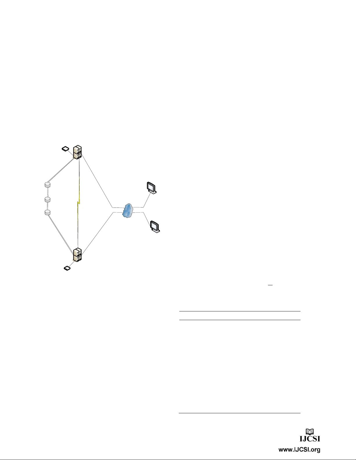
IJCSI International Journal of Computer Science Issues, Vol. 6, No. 2, 2009 ISSN (Online): 1694-0784 ISSN (Print): 1694 -0814 25 High A vailability Cluster System for Local Disaster Recovery with Markov Modeling Approach T.T.Lwin and T.Thein University of Computer Studies Yangon, Myanmar Abstract The need for high availabi lity (H A) and disaster r ecovery (DR) in IT environment is more stringent than most of the oth er sectors of enterprises. Many businesses require the availa bility of business-critical appli cations 24 hours a day, seven d ays a week, and can afford no data loss in the event of a dis aster. It is vital that the IT infr astructure is resilient with regard to disruption, even site failures, and tha t business operations can continue without significant impact. As a result, DR has gained great importance in IT. Clustering of multiple ind ustries standard servers together to a llow workload sharing and fail-over capabilities is a low cost appro ach. In this pap er, we present th e availability model through Semi -Markov Process (SMP) and also analyze the differenc e in downtime of the SMP m odel and the approximate Continuous Time Markov Chain (CTMC) model. To acquire s ystem availabilit y, we perform numerical analysis and SHARPE tool evaluation. Keywords: availability , cluster sys tem, local disas ter recovery, markov modeling 1. Introduction High availability clusters (also known as HA Clusters or failover Cl usters) are com puter clusters i mplem ented to provide high availability of services. They op erate by having redundan t computers o r nodes w hich are used to provide service when a system compone nt fails. A cluster is a collection of computer nodes -- independent , self-contai ned com puter system s working together – to provide a more reliable and powerful system than a single n ode alone [8]. Cl ustering has pro ven to be a very effective method for s caling to larg er systems for added perform ance, as well as providi ng highe r levels of availability and lower manage ment costs. For this reason, softw are pack ages su ch as I BM’s RS/6000 Cluster Technology [8] (i.e., Ph oenix) and Microsoft’s Cluster Services [5] (i.e., Wolf pack) are being used to build high availability systems. Disaster recovery solutions have gain ed popularity in the past few years because of their ability to tolerate disasters and to achieve the reliability and availab ility. 2. Related Work Hunter [5] described s ome system characteristics that benefit from clusteri ng and prese nted a two- node Microsoft Cluster Service (MSCS) cluster configuration and also presented an availability mod el of that syste m using Mark ov modeli ng techniques. In [1] they discussed high availability and disaster recovery solu tions, and de scribed how HA and DR solutions di ffer from one anothe r and ho w they can b e combined to provide the highest levels of resilien cy for IT infrastructures. Trivedi et. al [10] described an av ailability model for a high availability platform using a multi-level h ierarchical composition approach that mix es reliability block diagrams and Markov chains, so as to allow detailed behavior to be capt ured while avoiding stat e space explosion. Song et al [9] provided novel so lutions with three –key components, availability m odeling, model evaluation and data analysis and examined num erical solutio ns for Markov m odels on the uni formi zation method . This paper also presents a monitoring a nd data analy sis fram ework, which is responsible for failure analysis and av ailability reconfiguration. The semi-Markov decision model is a powerful tool i n analyzing seq uential decisi on process wit h random decision epoc hs [2]. They presented the application of Markov decision p rocess algorith m, a joint optimization of inspection rate and its co rresponding mainten ance policy are also presented. 3. System Architecture The architecture is based on a n active-passive high availability solution. Each service under high availab ility needs at least two identical servers: a primary host, on which the service run, one or m ore secondary hosts, a ble to recover the application. As a resu lt of failure detection, the active-passive roles are switched. A heartbeat keep- IJCSI Internati onal Journal of Com puter Science Issues, Vol. 6, N o. 2, 2009 26 alive system is used to monito r the health of the nodes in the cluster. A disaster recovery solution is typically composed of two nodes , one active and one p assive. The active node is us ually calle d master or pr oduction n ode, and the passi ve node is calle d secondary or standby node. During normal operation, the only working node is th e master node; in the event of a node f ailover or switchover, the standby no de takes over the product ion role, by takin g its IP num ber, and com pletely repl acing the mast er one. To maintain the standby node for failov er, the standby node contai ns homoge nous installa tions and appl ications: data and configurat ions must al so be constantly synchronized with the master node. Application Server A Application Server B Heartbeat LAN/WAN Boot Drive Boot Drive Private Data A Data B Figure1: System Fram ework If a crash occurs and if the data is not restored , it can have devastati ng conseque nces for a business. So it is imperative for companies to effectively backu p and recover data and protect them from huge losses in productivit y and downt ime. In this way, hardware exposure is mitig ated through physical hard ware redundan cy. Clustering provides high availability by protectin g against a node failure. Howev er, it does not prevent agai nst storage failures. Give n the size of typical cluster environments, multiple hard disks are used to build larg e storage arrays. In Network and System Administrat ion, when lar ge numbers of any one device are used, failure is expected. When a hard disk fails, application di sruption is unavoidabl e, as all the nodes i n the cluster coul d be using that one particula r disk as shar ed storage which cont ains all files. With the widesprea d use of co mputers, data i s becomi ng more and m ore important i n human li fe. But all kinds o f accidents and disasters occur frequently. Data corruption and data loss by vari ous disasters have become more dominant, accounting for over 60% [1] of data loss .Recent high-profile data loss has rais ed awar eness o f the need to plan for reco very of conti nuity. Many data disaste r tolerance technolog ies have b een employed to increase the availability of data and to redu ce the data damage caused by disasters [2]. A true disaster recovery solution is the ability to restore full systems quickly on available computing resources which may be local but may also be remote if the situation dictates and must allow reco ve ry from site-wide disasters. The primary site may be com pletely down, a sec ondary site located in a n on-affected area would be used to restore services until the primary site comes back online. 4. Modeling and Analysis We propose the two-com ponent syst em, one component i s considered as active and the other as a standby (spare) unit. The failure rates of the active unit and the standby unit are different, a nd also the e ffect of failure of the standby unit is different from that of the active unit. Assuming t hat, the time to restorat ion and reb oot are exponentially distributed with rate µ and β respectively. We consider a routine diag nostic that is run every T time units, intended to detect the laten t fault of the standby unit. While units’ failure and restoration times are exponentially distributed, the ro utine diagnostic time interval is not a continuous time Markov chain. The model for the system with the diagno stic routine is called a semi- Markov chai n. To solve thi s model, we could crudely approximate the time to the n ext diagnostic to be exponentially distributed with mean 2 T .Descriptions of the state are shown in table (1). Table (1): State Description for Transitions m odel State Descriptions 1 Both active and spare units are working 2 Protection switch fails to cover the failure of the active unit 3 When active unit fails, protection switch successfully restores servic e by the standby unit 4 The failure of the standby un it while the active unit is still working is detected immediately 5 The failure of the standby unit is not detected 6 The system is in failure state IJCSI International Journal of Com puter Science Issues, Vol. 6, N o. 2, 2009 27 Figure2 : State Transition Model λ =failure rate of an active unit λ s =failure rate of a standby unit µ =restoration rate of a failed unit c =coverage probability of an active unit c s =coverage probability of a standby unit T =time units to detect the latent fault of the standby unit We may compute the steady-state probabilities by first writing down the stead y-state balance equ ations of figure 2 are as follows: = + 4 3 P P µ µ () () 1 1 1 1 1 1 P c P c cP P c s s s s − + + + − λ λ λ λ (1) () ( ) 2 1 1 P P c s λ β λ + = − (2) 3 3 6 2 1 P P P P cP s λ µ µ β λ + = + + (3) () 4 6 5 1 2 P P P T P c s s λ µ µ λ + = + + (4) () 5 1 2 1 P T P c s s ⎟ ⎟ ⎠ ⎞ ⎜ ⎜ ⎝ ⎛ + = − λ λ (5) 6 5 4 3 2 2 P P P P P s s µ λ λ λ λ = + + + (6) The conservat ion equatio n of fi gure 2 is obtained by summing the probabilities of all states in the system and the sum of the equation is 1. 1 1 = ∑ = n i i P (7) Combining t he above-m entioned bala nce equation s with the conservati on equatio ns, and sol ving these simultaneous equations, we acquire the closed-form solutio n for the system. () () () () () () ( ) () () () 1 1 1 2 2 1 1 1 1 2 2 1 2 1 1 2 2 1 1 1 1 − ⎥ ⎥ ⎥ ⎥ ⎥ ⎥ ⎥ ⎥ ⎥ ⎥ ⎥ ⎥ ⎥ ⎥ ⎥ ⎥ ⎥ ⎥ ⎥ ⎥ ⎥ ⎥ ⎥ ⎥ ⎥ ⎥ ⎥ ⎥ ⎥ ⎥ ⎥ ⎥ ⎥ ⎥ ⎥ ⎥ ⎥ ⎥ ⎥ ⎥ ⎥ ⎥ ⎥ ⎥ ⎥ ⎥ ⎥ ⎥ ⎥ ⎥ ⎥ ⎥ ⎥ ⎦ ⎤ ⎢ ⎢ ⎢ ⎢ ⎢ ⎢ ⎢ ⎢ ⎢ ⎢ ⎢ ⎢ ⎢ ⎢ ⎢ ⎢ ⎢ ⎢ ⎢ ⎢ ⎢ ⎢ ⎢ ⎢ ⎢ ⎢ ⎢ ⎢ ⎢ ⎢ ⎢ ⎢ ⎢ ⎢ ⎢ ⎢ ⎢ ⎢ ⎢ ⎢ ⎢ ⎢ ⎢ ⎢ ⎢ ⎢ ⎢ ⎢ ⎢ ⎢ ⎢ ⎢ ⎢ ⎣ ⎡ ⎟ ⎟ ⎟ ⎟ ⎟ ⎟ ⎟ ⎟ ⎟ ⎟ ⎟ ⎟ ⎟ ⎟ ⎟ ⎟ ⎟ ⎟ ⎟ ⎠ ⎞ ⎜ ⎜ ⎜ ⎜ ⎜ ⎜ ⎜ ⎜ ⎜ ⎜ ⎜ ⎜ ⎜ ⎜ ⎜ ⎜ ⎜ ⎜ ⎜ ⎝ ⎛ + + + ⎟ ⎟ ⎟ ⎟ ⎠ ⎞ ⎜ ⎜ ⎜ ⎜ ⎝ ⎛ + − − − + − + + + − + + + − ⎟ ⎟ ⎠ ⎞ ⎜ ⎜ ⎝ ⎛ + + + + + + ⎟ ⎠ ⎞ ⎜ ⎝ ⎛ + − − − + − + ⎟ ⎟ ⎟ ⎟ ⎠ ⎞ ⎜ ⎜ ⎜ ⎜ ⎝ ⎛ + − − − + − + + − + − + = µ λ µ λ µ µ β λ β λ λ λ λ λ λ µ µ λ λ λ λ µ λ µ λ µ λ µ λ µ λ µ λ λ λ β λ β λ λ λ λ λ λ µ β λ λ s s s s s s s s s s s s s s s s s s s s s s s s s c c T T c c c c c c T T c c T c c c T T c c c P (8) ( ) 1 2 1 P c P s ⎟ ⎟ ⎠ ⎞ ⎜ ⎜ ⎝ ⎛ + − = β λ λ (9) IJCSI Internati onal Journal of Com puter Science Issues, Vol . 6, No. 2, 2009 28 () ( ) () () () () () 1 3 1 2 2 1 1 1 2 2 1 1 1 P c c T T c c c c T T c c c c c c P s s s s s s s s s s s s s s s s s s ⎟ ⎟ ⎟ ⎟ ⎟ ⎟ ⎟ ⎟ ⎟ ⎟ ⎟ ⎟ ⎟ ⎟ ⎟ ⎟ ⎟ ⎟ ⎟ ⎟ ⎟ ⎟ ⎟ ⎟ ⎠ ⎞ ⎜ ⎜ ⎜ ⎜ ⎜ ⎜ ⎜ ⎜ ⎜ ⎜ ⎜ ⎜ ⎜ ⎜ ⎜ ⎜ ⎜ ⎜ ⎜ ⎜ ⎜ ⎜ ⎜ ⎜ ⎝ ⎛ ⎟ ⎟ ⎟ ⎟ ⎠ ⎞ ⎜ ⎜ ⎜ ⎜ ⎝ ⎛ + − − − + − + + − + + + ⎟ ⎟ ⎟ ⎟ ⎠ ⎞ ⎜ ⎜ ⎜ ⎜ ⎝ ⎛ + − − − + − + + + − + + + − × + + = β λ β λ λ λ λ λ λ µ µ λ µ λ µ µ β λ β λ λ λ λ λ λ µ µ λ λ λ λ λ µ λ µ (10) () ( ) () () () 1 4 1 2 2 1 1 1 P c c T T c c c c c c P s s s s s s s s s s s ⎟ ⎟ ⎟ ⎟ ⎟ ⎟ ⎟ ⎟ ⎟ ⎟ ⎟ ⎟ ⎟ ⎟ ⎟ ⎟ ⎟ ⎟ ⎟ ⎠ ⎞ ⎜ ⎜ ⎜ ⎜ ⎜ ⎜ ⎜ ⎜ ⎜ ⎜ ⎜ ⎜ ⎜ ⎜ ⎜ ⎜ ⎜ ⎜ ⎜ ⎝ ⎛ + + + ⎟ ⎟ ⎟ ⎟ ⎠ ⎞ ⎜ ⎜ ⎜ ⎜ ⎝ ⎛ + − − − + − + + + − + + + − = µ λ µ λ µ µ β λ β λ λ λ λ λ λ µ µ λ λ λ λ (11) () 1 5 2 1 P T c P s s ⎟ ⎟ ⎟ ⎟ ⎠ ⎞ ⎜ ⎜ ⎜ ⎜ ⎝ ⎛ + − = λ λ (12) () ( ) () () () () 1 6 2 2 1 1 2 2 1 1 1 P T T c c c c T T c c c c c c P s s s s s s s s s s s s s s s ⎟ ⎟ ⎟ ⎟ ⎟ ⎟ ⎟ ⎟ ⎟ ⎟ ⎟ ⎟ ⎟ ⎟ ⎟ ⎟ ⎟ ⎟ ⎟ ⎟ ⎟ ⎟ ⎟ ⎟ ⎟ ⎠ ⎞ ⎜ ⎜ ⎜ ⎜ ⎜ ⎜ ⎜ ⎜ ⎜ ⎜ ⎜ ⎜ ⎜ ⎜ ⎜ ⎜ ⎜ ⎜ ⎜ ⎜ ⎜ ⎜ ⎜ ⎜ ⎜ ⎝ ⎛ ⎟ ⎠ ⎞ ⎜ ⎝ ⎛ + − − − + + + ⎟ ⎟ ⎟ ⎟ ⎠ ⎞ ⎜ ⎜ ⎜ ⎜ ⎝ ⎛ + − − − + − + + + − + + + − × + = λ µ λ µ λ µ λ µ λ µ µ β λ β λ λ λ λ λ λ µ µ λ λ λ λ µ λ µ (13) 4.1Semi-Markov Model Analysis A better approach would be to tak e the time the next diagnostic to be uniformly distributed ov er [0, T], resulting in a semi-Markov chain. T his is indicated in fig: 2 the transition labeled U (0, T). As occurring in two stages of transitions, the SMP is describe d by a transition probab ility matrix P and the vector of sojourn time distributions, H (t). ( ) t s e H λ λ + − − = 1 1 (14) ( ) t s e H λ β + − − = 1 2 (15) ( ) t s e H µ λ + − − = 1 3 (16) ( ) t e H µ λ + − − = 1 4 (17) (18) t e H µ 2 6 1 − = (19) Let X~EXP ( λ ) and Y~U (0, T) ra ndom variabl es ⎪ ⎩ ⎪ ⎨ ⎧ ≥ < ⎟ ⎠ ⎞ ⎜ ⎝ ⎛ − − = − , , 1 , , 1 1 5 T t T t e T t H t λ IJCSI International Journal of Com puter Science Issues, Vol. 6, No. 2, 2009 29 P(X>Y)= () ( ) ∫ > T Y dt t f t X P 0 = dt T e T t 1 0 ∫ − λ = () T e T λ λ − − 1 1 (20) The one-step transition probability matrix P of the DTMC em be dded at the time of transitio ns and the state probab ilities of the embedded DTMC are gi ven by the f ollowing e quations respect ively. 1 2 3 4 5 6 P= 1 2 3 4 5 6 () ( ) () () ⎥ ⎥ ⎥ ⎥ ⎥ ⎥ ⎥ ⎥ ⎥ ⎥ ⎥ ⎥ ⎥ ⎥ ⎥ ⎦ ⎤ ⎢ ⎢ ⎢ ⎢ ⎢ ⎢ ⎢ ⎢ ⎢ ⎢ ⎢ ⎢ ⎢ ⎢ ⎢ ⎣ ⎡ − − − + + + + + + + − + + + − − − 0 0 2 1 2 1 0 0 1 1 1 0 1 1 0 0 0 0 0 0 0 0 0 0 0 0 0 0 0 0 1 1 0 T T s s s s s s s s s s s s s s e T e T c c c c λ λ λ λ µ λ λ µ λ µ µ λ λ µ λ µ λ β λ λ β β λ λ λ λ λ λ λ λ λ λ λ λ (21) [ ] 0 , 0 1 1 , 0 1 1 , 1 , , , , v v v v v v D C = (22) To obtain the steady state probabilities, solve the equation v=vP (23) This yield () 1 2 1 v c v s λ λ λ + − = (24) () () () () 1 2 3 1 1 1 1 1 1 2 1 v c c c e T c v s s s T s s s s s s ⎥ ⎥ ⎥ ⎥ ⎥ ⎥ ⎥ ⎥ ⎥ ⎥ ⎥ ⎥ ⎥ ⎥ ⎥ ⎥ ⎥ ⎥ ⎥ ⎥ ⎦ ⎤ ⎢ ⎢ ⎢ ⎢ ⎢ ⎢ ⎢ ⎢ ⎢ ⎢ ⎢ ⎢ ⎢ ⎢ ⎢ ⎢ ⎢ ⎢ ⎢ ⎢ ⎣ ⎡ ⎟ ⎟ ⎟ ⎟ ⎟ ⎟ ⎟ ⎟ ⎠ ⎞ ⎜ ⎜ ⎜ ⎜ ⎜ ⎜ ⎜ ⎜ ⎝ ⎛ ⎟ ⎟ ⎟ ⎟ ⎠ ⎞ ⎜ ⎜ ⎜ ⎜ ⎝ ⎛ + − − − − − + + + + + + − + = − λ β β λ λ λ λ λ λ λ µ µ λ λµ µ λ µ µ µ λ λ (25) () ( ) () () () 1 2 4 1 1 1 1 1 1 2 v c c c e T c v s s s T s s s s s ⎥ ⎥ ⎥ ⎥ ⎥ ⎥ ⎥ ⎥ ⎥ ⎥ ⎥ ⎦ ⎤ ⎢ ⎢ ⎢ ⎢ ⎢ ⎢ ⎢ ⎢ ⎢ ⎢ ⎢ ⎣ ⎡ ⎟ ⎟ ⎟ ⎟ ⎟ ⎟ ⎟ ⎟ ⎟ ⎟ ⎟ ⎠ ⎞ ⎜ ⎜ ⎜ ⎜ ⎜ ⎜ ⎜ ⎜ ⎜ ⎜ ⎜ ⎝ ⎛ ⎟ ⎟ ⎟ ⎟ ⎟ ⎟ ⎟ ⎟ ⎠ ⎞ ⎜ ⎜ ⎜ ⎜ ⎜ ⎜ ⎜ ⎜ ⎝ ⎛ + − − − − − + + + + + + + = − λ β β λ λ λ λ λ λ λ µ µ λ λµ µ λ µ λ λ (26) ( ) 1 5 1 v c v s s s λ λ λ + − = (27) ( ) () () () () () ( ) 1 2 2 6 1 1 1 1 1 1 1 2 2 v c c c c c e T c v s s s s s s T s s s s s s ⎥ ⎥ ⎥ ⎥ ⎥ ⎥ ⎥ ⎥ ⎥ ⎥ ⎥ ⎥ ⎥ ⎥ ⎦ ⎤ ⎢ ⎢ ⎢ ⎢ ⎢ ⎢ ⎢ ⎢ ⎢ ⎢ ⎢ ⎢ ⎢ ⎢ ⎣ ⎡ + + − − + − ⎟ ⎟ ⎟ ⎟ ⎟ ⎟ ⎟ ⎟ ⎠ ⎞ ⎜ ⎜ ⎜ ⎜ ⎜ ⎜ ⎜ ⎜ ⎝ ⎛ ⎟ ⎟ ⎟ ⎟ ⎠ ⎞ ⎜ ⎜ ⎜ ⎜ ⎝ ⎛ + − − − − − + + + + + + − + = − λ β λ λ β λ λ λ λ λ β β λ λ λ λ λ λ λ µ µ λ λµ µ λ µ µ λ λ (28) IJCSI Internati onal Journal of Com puter Science Issues, Vol . 6, No. 2, 2009 30 The mean sojourn time i h in state i is () () dt t H h i i ∫ ∞ − = 0 1 (29) s h λ λ + = 1 1 (30) s h λ β + = 1 2 (31) µ λ + = s h 1 3 (32) µ λ + = 1 4 h (33) () T e T h λ λ λ − − − = 1 1 1 2 5 (34) µ 2 1 6 = h (35) The state probabilities of the semi-Markov chain are ∑ = j j j i i i h v h v π (36) , where ( ) () () {( ) } 0 , 0 , 1 , 0 , 1 , 1 , 0 , 1 , 1 , 1 , D C j i ∈ () () () () () () ( ) () () () () () () () () () () () ( ) 6 2 2 5 4 2 3 2 2 2 1 1 1 1 2 2 1 1 1 1 1 1 2 2 2 . 1 . 1 1 1 1 1 1 2 . 1 1 1 1 1 1 2 1 h c c c c c e T c h c h c c c e T c h c c c e T c h c h h s s s s s s T s s s s s s s s s s s s T s s s s s s s s T s s s s s s s ⎥ ⎥ ⎥ ⎥ ⎥ ⎥ ⎥ ⎥ ⎥ ⎥ ⎥ ⎥ ⎥ ⎥ ⎦ ⎤ ⎢ ⎢ ⎢ ⎢ ⎢ ⎢ ⎢ ⎢ ⎢ ⎢ ⎢ ⎢ ⎢ ⎢ ⎣ ⎡ + + − − + − ⎟ ⎟ ⎟ ⎟ ⎟ ⎟ ⎟ ⎟ ⎠ ⎞ ⎜ ⎜ ⎜ ⎜ ⎜ ⎜ ⎜ ⎜ ⎝ ⎛ ⎟ ⎟ ⎟ ⎟ ⎠ ⎞ ⎜ ⎜ ⎜ ⎜ ⎝ ⎛ + − − − − − + + + + + + − + + + − + ⎥ ⎥ ⎥ ⎥ ⎥ ⎥ ⎥ ⎥ ⎥ ⎥ ⎥ ⎦ ⎤ ⎢ ⎢ ⎢ ⎢ ⎢ ⎢ ⎢ ⎢ ⎢ ⎢ ⎢ ⎣ ⎡ ⎟ ⎟ ⎟ ⎟ ⎟ ⎟ ⎟ ⎟ ⎟ ⎟ ⎟ ⎠ ⎞ ⎜ ⎜ ⎜ ⎜ ⎜ ⎜ ⎜ ⎜ ⎜ ⎜ ⎜ ⎝ ⎛ ⎟ ⎟ ⎟ ⎟ ⎟ ⎟ ⎟ ⎠ ⎞ ⎜ ⎜ ⎜ ⎜ ⎜ ⎜ ⎜ ⎝ ⎛ + − − − − − + + + + + + + + ⎥ ⎥ ⎥ ⎥ ⎥ ⎥ ⎥ ⎥ ⎥ ⎦ ⎤ ⎢ ⎢ ⎢ ⎢ ⎢ ⎢ ⎢ ⎢ ⎢ ⎣ ⎡ ⎟ ⎟ ⎟ ⎟ ⎟ ⎟ ⎠ ⎞ ⎜ ⎜ ⎜ ⎜ ⎜ ⎜ ⎝ ⎛ ⎟ ⎟ ⎟ ⎟ ⎠ ⎞ ⎜ ⎜ ⎜ ⎜ ⎝ ⎛ + − − − − − + + − + + + − + + + − + = − − − λ β λ λ β λ λ λ λ λ β β λ λ λ λ λ λ λ µ µ λ λµ µ λ µ µ λ λ λ λ λ β β λ λ λ λ λ λ λ µ µ λ λµ µ λ µ λ λ β β λ λ λ λ λ λ λ µ µ λ λµ µ λ µ µ λ λ λ λ π λ λ λ (37) ( ) 1 1 2 2 1 h P h c s × + − = λ λ λ π (38) ( ) () () () 1 1 3 2 2 3 1 1 1 1 1 1 2 h h c c c e T c s s s T s s s s s s π λ β β λ λ λ λ λ λ λ µ µ λ λµ µ λ µ µ λ π λ × ⎥ ⎥ ⎥ ⎥ ⎥ ⎥ ⎥ ⎥ ⎥ ⎥ ⎥ ⎦ ⎤ ⎢ ⎢ ⎢ ⎢ ⎢ ⎢ ⎢ ⎢ ⎢ ⎢ ⎢ ⎣ ⎡ ⎟ ⎟ ⎟ ⎟ ⎟ ⎟ ⎟ ⎟ ⎠ ⎞ ⎜ ⎜ ⎜ ⎜ ⎜ ⎜ ⎜ ⎜ ⎝ ⎛ ⎟ ⎟ ⎟ ⎟ ⎠ ⎞ ⎜ ⎜ ⎜ ⎜ ⎝ ⎛ + − − − − − + + − + + + − + = − (39) IJCSI International Journal of Com puter Science Issues, Vol. 6, N o. 2, 2009 31 () ( ) () () () ⎥ ⎥ ⎥ ⎥ ⎥ ⎥ ⎥ ⎥ ⎥ ⎥ ⎥ ⎦ ⎤ ⎢ ⎢ ⎢ ⎢ ⎢ ⎢ ⎢ ⎢ ⎢ ⎢ ⎢ ⎣ ⎡ ⎟ ⎟ ⎟ ⎟ ⎟ ⎟ ⎟ ⎟ ⎟ ⎟ ⎟ ⎠ ⎞ ⎜ ⎜ ⎜ ⎜ ⎜ ⎜ ⎜ ⎜ ⎜ ⎜ ⎜ ⎝ ⎛ ⎟ ⎟ ⎟ ⎟ ⎟ ⎟ ⎟ ⎟ ⎠ ⎞ ⎜ ⎜ ⎜ ⎜ ⎜ ⎜ ⎜ ⎜ ⎝ ⎛ + − − − − − + + + + + + + = − s s s T s s s s s c c c e T c λ β β λ λ λ λ λ λ λ µ µ λ λµ µ λ µ λ π λ 1 1 1 1 1 1 2 2 4 (40) () 1 1 5 5 1 h P h c s s × + − = λ λ λ π (41) ( ) () () () () () ( ) 1 1 6 2 2 6 1 2 2 1 1 1 1 1 1 2 h P h c c c c c e T c s s s s s s T s s s s s s × ⎥ ⎥ ⎥ ⎥ ⎥ ⎥ ⎥ ⎥ ⎥ ⎥ ⎥ ⎥ ⎥ ⎥ ⎦ ⎤ ⎢ ⎢ ⎢ ⎢ ⎢ ⎢ ⎢ ⎢ ⎢ ⎢ ⎢ ⎢ ⎢ ⎢ ⎣ ⎡ + + − − + − ⎟ ⎟ ⎟ ⎟ ⎟ ⎟ ⎟ ⎟ ⎠ ⎞ ⎜ ⎜ ⎜ ⎜ ⎜ ⎜ ⎜ ⎜ ⎝ ⎛ ⎟ ⎟ ⎟ ⎟ ⎠ ⎞ ⎜ ⎜ ⎜ ⎜ ⎝ ⎛ + − − − − − + + − + + + − + = − λ β λ λ β λ λ λ λ λ β β λ λ λ λ λ λ λ µ µ λ λµ µ λ µ µ λ π λ (42) 5. Experimental Results The exact model param eter values for the model are not known, however, a good estimate valu e for a range of model param eter is assumed. Fi g: 3 plots t he difference between dow ntime (mi nutes per year) estim ates obtained using the SM P model and that obt ained by a pproxim ating the U (0, T) dist ribution by an expone ntial dist ribution with mean T/2. We take the values c=0.9, c s =0.9, µ=1per hour, β =12 per hour, and λ s = λ /4. We see that the higher the µ/ λ ratio, the lower the downtime compu ted by the two models. Availability models cap ture failure and repair behavior of systems and their com ponents. States of the und erlying Markov chain will be classified as up states or down states. The system is not available in the state 2 and state 6. T he system availability in the stead y-state is defined as follows: Availability=1-Unavailability =1-( π 2 + π 6 ) (43) 0.00000 10.00000 20.00000 30.00000 40.00000 1234 Down ti m e DT ( ct m c) DT ( smp) Figure3:Difference in downtime of the SMP m odel and the approximate CTMC m odel 5.1 Validation of Closed-form Results To verify the validity o f our form ula derivati ons, we compare the results obtained from the closed-form solution and the results obtained from th e numerical solution by SHARPE. We found th at our results are same. 0.00000 10.00000 20.00000 30.00000 40.00000 1234 DT D T ( der iv at ion) DT( S HA RP E ) Figure4: Downtime of the CTMC model 0. 00000 5 . 00000 1 0. 00000 1 5 . 000 00 20. 00000 25 . 0 0000 30. 00000 35 . 0 0000 12 3 4 DT( S HA RP E) D T ( der i v at ion) Figure5: Downtime of the SMP model IJCSI Internati onal Journal of Com puter Science Issues, Vol . 6, No. 2, 2009 32 6. Conclusion Organizations today face a to ugh c hallenge in choosing an appropriate high availabil ity solution that meets their business requirements and IT budgets. To im plement this requirement, organizations must give high availability and disaster recovery. High availability systems require fewer failures and fa ster repair. In this paper we present ed high availability cluster and failover availability for disaster events. . We present a Markov m odel and expres s availability and downtime in terms of the parameters in the model. We evaluate th e feasibility of our clus tering model using SHAR PE tools. References [1] D. Clitherow, M. Brookbanks, N. Clayton, and G . Spear, ‘‘Combining High Availability and Disaster Recovery Solutions for Critical IT Environments,’’ IBM Systems Journal 47, No. 4, 563–575 (2008) [2] D.Chen, K.S.Trivedi,”Op timization for condition-based maintenance with semi-Markov decision process” Available online at www.sciencedirect.com [3] R. Gamache, R Short, and Mike Massa, "Windows NT Clustering Service," IE EE Computer, October 1998, pp.55-61. [4] C.Hirel, A. Robin, Sa hner, X.Zang, K.S.Triv edi: “Reliability and performi ng modeling using SHARPE 2000”. Computer Performance Evaluation/TOOLS 2000. In Lecture Notes in Computer Science; V ol.1786, Springer-Verlag, 2000, pp.345-349. [5] S. W. Hunter and W. E. Smith, “Availabili ty Modeling and Analysis of a Two Node Clu ster,” Proceedings of the 5th International Conference on Information Systems, Analysis and Synthesis, Orlando, FL, October 1999. [6] Th. Lumpp, J. Schneider, J. Holtz, M. Mueller, N. Lenz, A. Biazetti, and D. Petersen, ‘‘From High Availabi lity and Disaster Recove ry to Business Continuity Solutions,’’ IBM Systems Journal 47, No. 4, 605–619 [7] M.Malhotra, A.Reibman: ”Selecting and Implementing Phase Approximations for Semi-Markov Models”, Volume 9, Issue 4, 1993, Pages 4 73-506. [8] G.F. Pfister, In Search of Clusters: The Coming Battle in Lowly Parallel Computing, Prentice Hall, Eng lewood Cliffs, NJ, 1998. [9] H.Song, C.Leangsuksun, R.Nassar, “Availability Modeling and Evaluation on High Performance Cluster Computing Systems,” Journal of Research and Practice in Information Technolog y, Vol.38, No.4, November 2006. [10] K. S. Trivedi, R. Vasiredd y, D. Trindade, S. Nathan, and R. Castro. Modeling high avai lability systems. In Proc. Pacific Rim Dependabi lity Conference, 2006. [11] K.S.Trivedi:” Probabilit y and Statistics with Reliabil ity, Queuing, and Computer Sc ience Applications”, John Wiley and Sons, 2002. [12] M.Wiboonrat, “Transformatio n of System Failure Life Cycle,” Inte rnational Journa l of Management Science and Engineering Management, Vol.4 (2008) No.2, pp.143-152.