Entropic Priors and Bayesian Model Selection

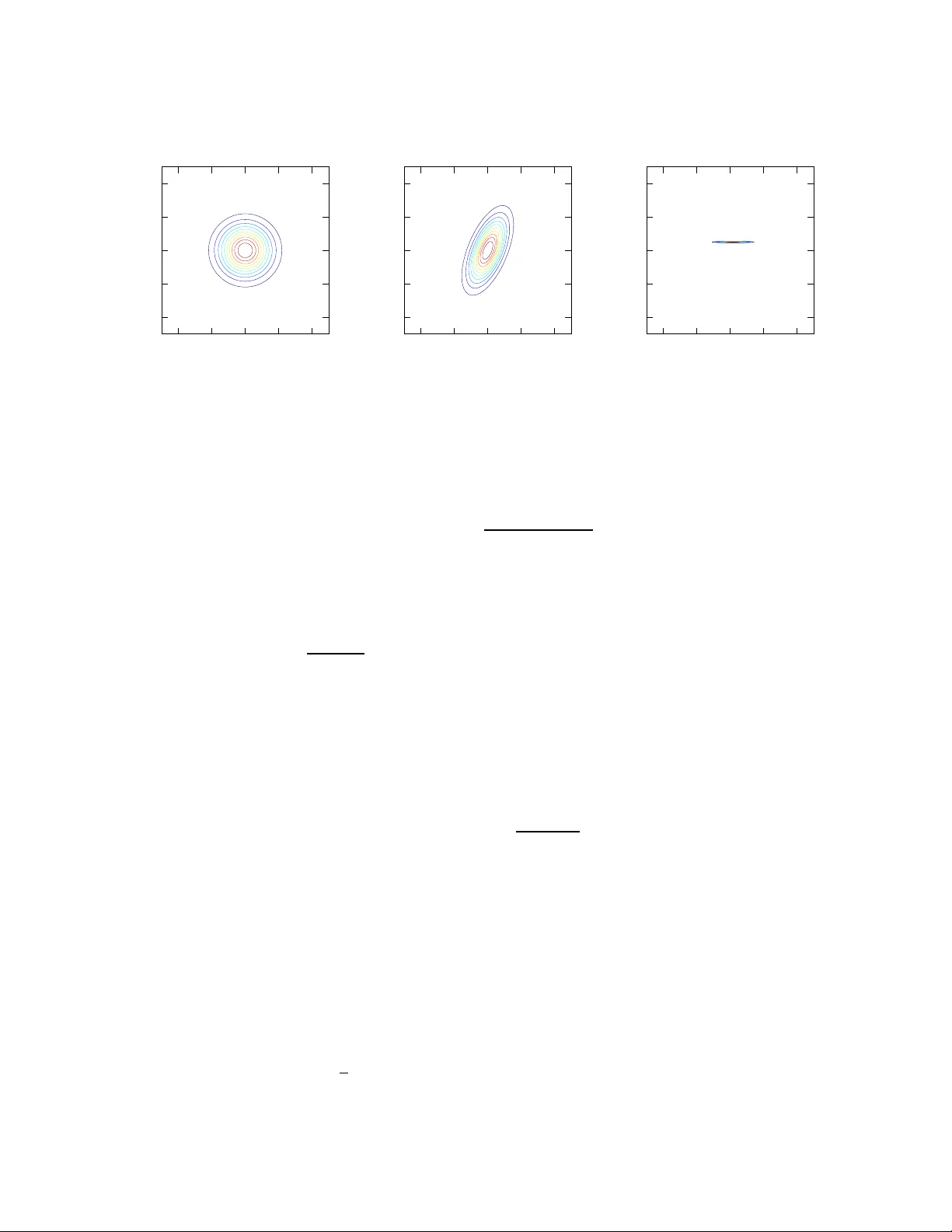
Entr opic Priors and Bayesian Model Selection Brendon J. Brewer 1 ∗ and Matthe w J. Francis † ∗ Department of Physics, University of California, Santa Barbara, CA, 9310 6-953 0, USA † SiSSA, via Beirut, 2-4 3415 1 T rieste TS, Italy Abstract. W e demonstra te that the princip le of maximu m relati ve entropy (ME), used jud iciously , can ease the specification of pr iors in model selection problems. The resultin g effect i s th at models that make sharp predictions are disfa voured, weakening t he usual Bayesian “Occa m’ s Razor”. This is illustrated with a simp le example i nv olving what Jay nes called a “sure thing” h ypothesis. Jaynes’ r esolution of the s ituation in volved introdu cing a large number of alternati ve “sure thing” hypoth eses that were p ossible bef ore we observed the data. Howe ver, in m ore comp lex situations, it may not be possible to explicitly enumera te large numbers of alternativ es. The en tropic prio rs formalism pro duces the desired resu lt without modify ing the hypoth esis space or r equiring explicit enumera tion of alternatives; all that is required is a good mo del for the prior pred icti ve distribution for the data. Th is id ea is illustrated with a si mple rigged-lottery example, and w e outline h ow this idea may help to resolve a re cent d ebate amo ngst cosmo logists: is d ark energy a cosmological constant, or has it ev olved wit h time in some way? And how shall we decide, when the data are in? Keywords: Inferen ce, Model Selection, Dark Energy P A CS: 0 2.50.T t, 89.70.Cf, 95.36.+x 1. INTR ODUCTION In Bayesian model selection, we hav e two or more competing hypotheses, H 1 and H 2 , wit h each pos sibly containing di f ferent parameters θ 1 and θ 2 . W e wish to jud ge the plausibilit y of t hese two hypotheses in the light of some data D , and some prior information I , dropped hereafter for succinct ness. Bayes’ rule provides the means to update our plausibilit ies of these tw o model s, to take into a ccount the data D : P ( H 2 | D ) P ( H 1 | D ) = P ( H 2 ) P ( H 1 ) P ( D | H 2 ) P ( D | H 1 ) = P ( H 2 ) P ( H 1 ) × R p ( θ 1 | H 1 ) p ( D | θ 1 , H 1 ) d θ 1 R p ( θ 2 | H 2 ) p ( D | θ 2 , H 2 ) d θ 2 (1) Thus, the ratio of the posterior probabilities for t he two mod els is the prior odds ratio times the e vidence ratio. If the v ario us probabilities on the right-hand s ide of Equation 1 are a good description of our prior beliefs, t hen the post erior probabiliti es will encode justified conclu sions based on the data. Howe ver , practical use o f Eq uation 1 is often regarded with scepticism [5, 9, 10]. This is primarily because the probabi lities on th e right-hand si de are difficult to specify without making ad hoc choices. For reasons that are most ly histo rical, the prior distributions p ( θ 1 | H 1 ) and p ( θ 2 | H 2 ) for the parameters of each model are usually considered the mo st troubling. The prior 1 Email: brewer@physic s.ucsb.edu model probabilities are often set to 1 / 2 , c iting symmetry , and the sam pling distri butions are us ually considered uncontrov ersial. Howe ver , in many real s cientific applicati ons, assigning p riors is trivial compared to the job of assign ing s ampling di stributions (Hogg, priv comm); i.e. modell ing ho w the question of interest would a ffect our data. While many Bayesians would assert that the depend ence on sub jectiv e judgm ents exists bec ause t he result should actually depend on these jud gments, it seems as th ough there o ught to be ways to reduce the subjective influences in the prior probabiliti es and sampling distributions, e ven i f they can never be ent irely elimi nated. In fact, this is t he entire reason for us ing Bayes’ rul e i n the first place [11]. Rather than simply loo king at the data and then ass igning a po sterior distribution directly , we make use of one obj ecti ve thing we actuall y know , Bayes’ rule. In this paper , we di scuss h ow the principle o f maximum r elative entropy (ME) [3] can be used to further reduce, though not eliminate, the subjectivity of Bayesian inferences. The k ey requirement of thi s approach is th at we must have a r ealistic probabilistic model of our prior beliefs about the data, i.e. our prio r predictiv e distribution for the data must be modelled carefully . 1.1. Publishing the Eviden ce Skilling [16] recommends that whenever some data is analysed using a model M 1 , the e vidence Z 1 = p ( D | M 1 ) = R p ( θ 1 ) p ( D | θ 1 ) d θ 1 be presented. T his way , anyone propos ing a diffe rent model M 2 can calculate their own e vi dence Z 2 and carry out model comp ari- son with Equation 1 without t he need to recalculate Z 1 , which was published by the first author . This i s good a dvice that has bee n taken by m any in the astronomical community [17, 18], howe ver , it is not the whole story . The plausibilit y of a model does not depend only on the evidence, it also depends on the prior probabili ty (Equation 1). A large evi- dence ratio can easily be cancelled by a t iny pri or probability ratio and vice versa. T he sure thing problem, dis cussed in Section 2, is simp le and well-known example of this fact. 2. A SURE THING PR OBLEM Suppose a simple lottery is held, wit h tickets numbered from 1 to 1,000,0 00. Each tick et is sold to a different person. Consider a hypoth esis H 1 , which st ates that the lottery is fair , and thus the probabi lity of an y p articular ticket wi nning is 10 − 6 . The draw is c arried out, producing the following data D : The win ner o f t he lottery was ticket # 263878. Alice publishes a paper that reports this data, and p roposes the f air lottery model H 1 to explain it. She presents the e vidence Z 1 = P ( D | H 1 ) = 10 − 6 . Bob, a professional riv al of Alice, reads her paper and proposes a different m odel, H 2 : The lott ery was n ot fair . It was rigged in order to m ake ticket #263 878 the winner . Bob writes a paper presenting the evidence Z 2 = P ( D | H 2 ) = 1. Thus, he concludes, if H 1 and H 2 are initially equally plausible, the data makes H 2 a m illion times more plausible than H 1 . Clearly , som ething is not quite right with this conclusion. 2.1. Jaynes’ Solution: Intro duce extra hypotheses Jaynes [6] resol ves the sure thing paradox in t he following way . When Bob does a model selectio n between H 1 and H 2 with P ( H 1 ) = P ( H 2 ) = 1 2 , he is impli citly stating that before getti ng the data, he would h a ve predicted ticket #263 878 with a prob ability greater than 5 0 %. Clearly , there i s no way he could have kno wn thi s before seeing the data. Actually , before obs erving t he data, there were 999,999 other “sure thi ng” hypotheses that were on an equal footing with H 2 . The correct analysis would in volve a bigger hypo thesis space containing 1,000,001 hypo theses: H 1 , and the 1,000 ,000 sure thing hy potheses { S 1 , S 2 , ..., S 1 , 000 , 000 } , wh ere S 263878 ≡ H 2 . Bob shoul d hav e assign ed 1/2 of the prior probabilit y to H 1 and divided the other 1/ 2 e venly amo ngst the S ’ s. Then, the prior probability of H 2 is 5 × 10 − 7 and it s posterior p robability i s 1 / 2. Th is is the correct result; knowledge of the winning ticket number does not af fect the plausibili ty of foul pl ay . This ar gument resolves th e sure t hing problem by introducing a lar ge number o f al ternativ es into the hypothesis sp ace, thus drastically reducing the prior probability of the particular sure t hing hypoth esis selected by the data. Ho wev er , it is diffic ult t o generalise this reasoning in to m ore compli cated scenarios where the principle of indif ference cannot be used. Before the lottery was drawn, Bob would ha ve assigned a uniform predictiv e dis tri- bution for the data. His reanalysis ought to reflect this, if not by introducing extra sure thing m odels, then by downweighting H 2 somehow to reduce the s pike it produces in the predicti ve distribution. While this is not the explicit moti vation for entropic priors, it is a pleasant side ef fect, as we will show in th e next section. 3. ENTROPIC PRIORS In thi s section we introduce the no tion of an entropic p rior [4, 14]. Usuall y , Bayesian Inference is concerned wi th describi ng our knowledge in two stages: before taking i nto account the data, and then after taking into account the data. Bayes’ rule is used to do this updating. Before taking int o account the data, there is a prior distribution p 1 ( θ ) and sampling distri butions p 1 ( D | θ ) for all D and θ . The reason for t he subscript ‘1’ will become clear lat er . By the product rule, this is equiv alent to defining a joint prior on the product space of possible hypotheses and possible data: p 1 ( θ , D ) = p 1 ( θ ) p 1 ( D | θ ) (2) Here, the usual prio r p 1 ( θ ) (actually a marginal distrib ution ) describes prior knowledge about θ , and the sampling distributions p 1 ( D | θ ) describe prior knowledge about how θ is related to the data D that we plan to ob serve. The k ey point here is that before l earning the data, we are u ncertain both about th e parameters and about the data: p 1 ( θ , D ) should model this state of uncertainty . In this paper , we will be concerned w ith d escribing uncertain knowledge about ( θ , D ) , so we will be us ing probabi lity d istributions on the product space. W e will st art from a joint prior p 0 ( θ , D ) and update this d istribution twice to obtain the final joi nt pos terior . W e thus describe kno wledge at three stages, defined below . • Stage 0: Before we observe the data, or ev en know what samplin g distrib ution s are. Ho wev er , the parameter space and the data space ha ve been defined, as well as priors ove r these spaces. At stage 0, our knowledge is p 0 ( θ , D ) . • Stage 1: Al so before we observe the data. Howe ver , we have no w specified the sampling di stributions p ( D | θ ) for all θ and D . At stage 1, our kn owledge is p 1 ( θ , D ) . • Stage 2: W e now have the dat a. Our kno wledge is p 2 ( θ , D ) . Updating from Stage 1 to Stage 2 is w hat we typically t hink of as Bayesian analysis. W e prefer updat ing, rather than jus t writin g down Stage 2 prob abilities, because we get to u se an ob jectiv e updating rule, Bayes’ rule. The idea behind entropi c priors is to split up th e process o f assigning Stage 1 prob abilities into two steps : Assigning Stage 0 probabil ities, and then updating to Stage 1 us ing anot her objective updating rule, ME [3]. There is a lot of confusion in the lit erature about the relationship between these two principles. Howev er , there need not be any tensio n between them if it is und erstood that Bayes’ rule is to b e used when we learn abou t proposit ions built from those in t he product space, such as ‘ D = 42’ or ‘ θ + D ≤ 1’, whereas ME app lies to propos itions about pr obab ility di stributions on that space 2 , such as ‘ p ( θ , D ) shoul d be a Gaussian’. 3.1. Updating from Stage 0 to Stage 1 Say we ha ve a Stage 0 join t prior , and we don’t know the sampli ng distributions yet. Perhaps we haven’ t calibrated the instruments t o see wh at kinds of output they typicall y produce. At this p oint our knowledge of ( θ , D ) will often be ind ependent, such th at taking data before learning about the e xperiment does not tell us anything about the pa - rameters (it does tell us the data - and is therefore signi ficant information in th e product space. Howe ver , data is usually a n uisance parameter[!]). Howe ver , for generality w e will allo w dependence in the stage 0 distribution: p 0 ( θ , D ) = p 0 ( θ ) p 0 ( D | θ ) . W e then learn information in the form of a constraint on allowable join t pr o babil- ity d istributions : the sampl ing d istributions p ( D | θ ) for all θ and D are given to us: p ( D | θ ) = f ( D ; θ ) , where f is a gi ven function. W e must adjust our joint distrib ution so that this constraint is satis fied. By the rules of probabil ity any d istribution of the form p 1 ( θ , D ) = p 1 ( θ ) f ( D ; θ ) is allo wed, and we ha ve absolut e freedom to vary p 1 ( θ ) whil e still satisfyin g the constraint on the samplin g dis tributions. Howe ver , there is a best choice for p 1 ( θ ) [3]: p 1 ( θ ) should be chos en such that p 1 ( θ , D ) is as close as possib le to p 0 ( θ , D ) , i.e. we choose the p 1 ( θ ) that maxim ises the relati ve entrop y S = − Z Z p 1 ( θ , D ) log  p 1 ( θ , D ) p 0 ( θ , D )  d θ d D (3) 2 This raises a philosophical p oint, as most inf ormation is ultimately in the for m of d ata. Howe ver , we may sum marise the resu ltant effect o f a large amoun t of external data as p roviding a constraint on our probab ility distributions. -4 -2 0 2 4 -4 -2 0 2 4 y x p 0 (x,y) -4 -2 0 2 4 -4 -2 0 2 4 y x p 1 (x,y) -4 -2 0 2 4 -4 -2 0 2 4 y x p 2 (x,y) FIGURE 1. The basic idea be hind en tropic priors. An initially indepe ndent N ( 0 , 1 ) joint p rior for two quantities x and y (to be thought of as “parameters” and “data” respectively) is upda ted once the s amplin g distributions p ( y | x ) ∀ y , x are kn own to be p ( y | x ) ∼ N ( x , 1 ) . W hen the data are known (in th is case, y = 0 . 5), the joint distribution is updated again. This second updating is equiv alent to the usual Bayesian process. = − Z Z p 1 ( θ ) p 1 ( D | θ ) log  p 1 ( θ ) p 1 ( D | θ ) p 0 ( θ ) p 0 ( D | θ )  d θ d D (4) Diffe rentiating with respect to each value o f p 1 ( θ ) (i.e. it s value at each θ ) and setting to zero (with Lagrange multipli er term added): ∂ ∂ p 1 ( θ )  S − λ  Z p 1 ( θ ) d θ − 1  = 0 (5) Carrying out this calculation giv es: p 1 ( θ ) ∝ p 0 ( θ ) e S ( D | θ ) (6) where S ( D | θ ) = − Z p 1 ( D | θ ) log  p 1 ( D | θ ) p 0 ( D | θ )  d D (7) Thus, the mar ginal for θ after learning the sampling distributions, p 1 ( D | θ ) , is propor- tional to t he original marginal p 0 ( θ ) , b u t mul tiplied by the e x ponential of the entropy of the corresponding sampl ing distribution relative to p 0 ( D | θ ) (usually jus t p 0 ( D ) ). This process of updating from s tage 0 to stage 1 u sing ME, and su bsequently updating using data, is illustrated graphically in Figure 1. Applying sim ilar logic to model selection probl ems consists simp ly of applying the short-cut reasoning of t he above paragraph: each hypot hesis (model and its parameter value) gets its prior probability rescaled by a factor measuring the closeness of its predictions to our ini tial p redictions. This makes it clear that i n voking s ymmetry to assign P ( H 1 ) = P ( H 2 ) = 1 2 is fla wed: the sy mmetry may be broke n as soon as we assign the sampling distributions. 4. SURE THING PR OBLEM: ENTRO PIC PRIORS SOLUTION For the lo ttery problem, our kn owledge about the data before getting it, and before the two m odels ha ve been specified, i s described by a u niform distri bution o ver the integers from 1 to 10 6 : p 0 ( D ) = 10 − 6 for all D 3 . Because t he two m odels haven’ t been specified yet, symmetry im plies we m ust assign equal prior (marginal s tage 0) probabilities p 0 ( H 1 ) = p 0 ( H 2 ) = 1 2 . The joint prob abilities for t he hypot hesis and the data are therefore uniform and independent. The next s tep is to incorporate more informati on and update our probabil ities t o stage 1. This information is not the data, but the specification o f the s ampling di stributions: p ( D | H 1 ) = 10 − 6 for all D , and p ( D | H 2 ) = 1 i f D = 263878 and zero otherwise. As explained in Section 3, the priors for th e two hypotheses should be re weighted according to t he exponential of the entropy of t heir samp ling dist ributions with respect to the original predicti ve distribution. These entropies are S ( D | H 1 ) = − 10 6 ∑ i = 1 10 − 6 log 10 − 6 10 − 6 = 0 (8) S ( D | H 2 ) = − 1 log 1 10 − 6 = lo g ( 10 − 6 ) (9) (10) Thus, the solution to the lottery problem is: p ( H 2 | D ) p ( H 1 | D ) = 1 2 1 2 ! ×  10 − 6 1  ×  1 10 − 6  = 1 (11) The th ree factors here are t he Stage 0 odds ratio, the entropic correction factor , and the evidence rati o. The resulti ng conclusion is as it shoul d be: knowing the winning lottery number pro vides no in formation about whether there is fraud or not. Usual ly , models that make sharp, correct predictions are fa voured by Bayesian inference. In thi s example, t his still occurs in the evidence ratio, b ut the entropic factor also penali zes H 2 by the sam e amount for being unjusti fiably confident compared t o our honest prior predictiv e distribution p 0 ( D ) . 5. EV OL VING D ARK ENE RGY The nature of dark ener gy , thought to be responsi ble for causing the observed late- time accelerated expansion of the Uni verse [12, 13], is a ke y drive r of m any upcom ing cosmological surveys and instrum ents [1]. From a model selection point of vie w , one 3 This co uld be d ifferent if we tr ied to incor porate psycholog ical theories as to which numbe rs would be more likely u nder the ch eating scenario - perhap s ‘ 12345 6’ would have its pro bability boo sted - but we will ignore this effect here. of th e key q uestions i s whet her th e equati on o f st ate of dark energy , w , is exactly equal to minus one for all ti me or whether it h as any temporal variation. Th e former case is equiv alent to Ei nstein’ s cosmolog ical constant, or non -zero vacuum ener gy , while any var iation from this value, howev er sm all, indicates very di f ferent physics at play , such as the existence of a primordial scalar field, or other ev en more exotic possibil ities [2]. Here, model selection is really the ke y goal; the exact form of an y e volution of w is less interesting t han si mply bein g sure that it does ev olve, or at least hav e a value different from the cosmological constant. There has been vigorous debate i n the li terature on ho w to best answer th is q uestion [5, 9, 10]. Here we outlin e th e contri bution entropic priors can make to this debate; detailed analysis will be pre sented in a future contribution. W e will consider fou r di f ferent models for how the dark energy equati on of state has var ied throu ghout the un iv erse’ s hi story . T ypically this i s described as w v arying as a function of a , the scale factor . H 0 : Cosmological Constant Λ : w ( a ) = − 1 H 1 : Constant, but non- Λ : w ( a ) = w 0 H 2 : Simple Evolving : w ( a ) = w 0 + ( 1 − a ) w a H 3 : Complex Evolving : w ( a ) = Some model with many parameters Observations of t ype Ia s upernov ae, particul arly how their apparent brightness decreases with redshift, is a s trong probe of w [8, 15]. The idea is to test the four m odels, given such data [5], and t o forecast the i nformative ness of p roposed future m issions [1]. Howe ver , not all of the models are physically well-motiv ated: e.g. H 0 arises naturall y from General Relativity , H 1 and H 2 are ad hoc “simple models”, and H 3 expresses gross ignorance. Therefore, wh ile it is fair to ass ign a large probabilit y to H 0 at Stage 1, it does n ot automaticall y make sense to share t he remaining probabil ity e venly amongst H 1 - H 3 . The reason for this is that H 1 , H 2 and H 3 may i mply qu ite di f ferent predicti ve distributions for the data. If we build a p 0 ( D ) that we trust, then the simple m odels H 1 and H 2 may be downgraded in prior probabilit y solely because they make predictions that are too confident 4 . Of course, i f, in the course of building p 0 ( D ) , we explicitly think about the predictions of t he H ’ s , then this will not occur - entropic prio rs do n ot magically generate information. What they do is i mplore us to t hink about p ( D ) when assig ning priors, a key sanity check that is often overlooked. 6. CONCLUSIONS Bayesian model selection is a difficult task, both computati onally and philosophi cally . If we are not careful, we ca n obtain misleading results. The idea presented in this paper , of assi gning a realistic predictiv e dist ribution for the data and then penali zing m odels whose prediction s diff er from it, s hould assi st in making Bayesian m odel selection analyses more reliable. 4 The chance that an unknown func tion just happens to be a straight line is usually quite small, u nless yo u have very good prior reasons to expect a straight line. REFERENCE S 1. Albrecht, A., and 10 c olleagues 200 9. Finding s of the Joint Dark E nergy Mission Figure of M erit Science W orking Group . Ar Xi v e-prin ts arXi v:090 1.072 1 . 2. Barnes, L., Francis, M. J., Lewis, G. F ., Linder, E. V . 2 005. The Influence of Evolving Dark E nergy on Cosmology . Publications of the Astronomical Society of Australia 22, 315-32 5. 3. Caticha, A., Lectures on Prob ability , E ntropy , and Statistical Physics. In vited lectures at MaxE nt 2008, th e 2 8th Intern ational W orksh op on Bayesian Inference and Maxim um En tropy Meth ods in Science an d Engine ering (July 8-1 3, 2008 , Boraceia Beach, Sao Paulo, Brazil). A vailable online at http://arxiv .org/abs/080 8.0012 4. Caticha, A., Preuss, R. 2004. Maximum en tropy and B ayesian data analy sis: Entropic p rior distribu- tions. Physical Re v iew E 70, 046127. 5. Efstathiou, G. 20 08. Limitation s of Bayesian Evid ence applied to cosmo logy . Monthly N otices o f the Royal Astronomical Society 388, 1314-13 20. 6. Jaynes, E. T ., ed. Brettho rst, G. L. 2 003. Probability Theory: The Logic of Science. Cambridge University Press. 7. K omatsu E., et al., 2009, ApJS, 180, 330 8. K ow alski, M., an d 69 colleagu es 2008. Improved Cosm ological Constraints fro m New , Old, an d Combined Supernova Data Sets. Astrophy sical J our nal 686, 749-778. 9. Liddle, A. R, Stefano Corasaniti, P ., Kunz, M., Mukh erjee, P ., Parkinson, D., Trotta, R. 200 7. Comment on ‘T ainted evidence: cosmological model selection versus fitting’, astro-ph/07 03285 . 10. Linder, E. V ., Miquel, R. 2007. T ainted Evidenc e: Cosmologica l Model Selection vs. Fitting. arXiv:astro-ph/070 2542 . 11. O’Hagan, A., Forster, J. 2004 . Kendall’ s advanced th eory of statistics. V ol.2B: Bayesian in ference, 2nd ed., by A. O’Hagan and J. Forster . Lon don: Hodder Arnold, 2004. 12. Perlmutter, S., a nd 32 colleagu es 1 999. Measuremen ts of Omega and Lamb da fr om 42 Hig h-Redshift Supernovae. Astroph ysical Jou rnal 517, 565-586 . 13. Riess, A. G., and 1 9 colleagues 1998 . Observ ational Evidence from Supe rnovae for an Accelerating Universe and a Cosmolog ical C onstan t. Astronomical Journal 116, 1009-10 38. 14. Rodrigu ez, C. 20 02. En tropic Priors for Discrete Pro babilistic Ne tworks a nd f or Mixture s of Gau s- sian Mo dels, in Bayesian I nference an d Ma ximum Entr opy Method s in S cience and En gineering , ed. by R. L. Fry , AIP Conf.Proc. 617, 410 (2002). 15. Rubin, D., and 23 colleagues 2 009. Loo king Beyond Lamb da with th e Un ion Super nova Compila- tion. Astrophysical Journal 695, 391-403 . 16. Skilling, J. 2006 . Nested Samplin g fo r Gener al Bayesian Com putation. Baye sian An alysis 1 , Nu mber 4, pp. 833-86 0. 17. T rotta, R. 2008. Baye s in th e s ky: Bayesian i nfer ence and m odel s election in cosmology . C ontem po- rary Physics 49, 71-104 . 18. V egetti, S., K oop mans, L. V . E. 200 9. Bayesian strong gr avitational-lens modelling on adap tiv e gr ids: objective de tection of mass substructu re in Ga laxies. Mon thly Notices of th e Royal Astro nomical Society 392, 945-963 . A CKNO WLEDGMENTS BJB would like t o thank the following for v alu able discussion: David W . Hogg, John Skilling, Ariel Caticha, Adom Giffin, Iain Murray , Phil Marshall and Geraint Lewis. I w ould also li ke to thank Geor gin a W ilcox for introducing me to mercurial , and T ommaso T reu for suppo rting my trip to Oxford, Mississippi.