Operator theory of electrical resistance networks

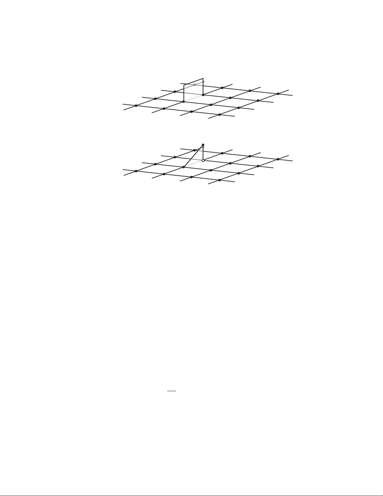
O P E R A T O R T H E O RY A N D A N A L Y S I S O F I N FI N I T E N E T W O R K S 1 − 1 + 1 + 2 3 0 2 1 + 2 1 + 3 1 + 12 1 + 6 1 + 4 1 + n 1 + n +1 1 + n ( n +1) 1 6 1 1 12 25 Σ k k =1 n 1 P A L L E E . T . J O R G E N S E N A N D E R I N P . J . P E A R S E Contents 1 Preface . . . . . . . . . . . . . . . . . . . . . . . . . . . . . . . . . . . . . . v 2 Note to the reader . . . . . . . . . . . . . . . . . . . . . . . . . . . . . v 3 Brief o verview of con tents . . . . . . . . . . . . . . . . . . . . . . . . . vii 4 In tro duction . . . . . . . . . . . . . . . . . . . . . . . . . . . . . . . . . . . . xi 5 Detailed description of conten ts . . . . . . . . . . . . . . . . . . . . . . xii 6 What this b ook is ab out . . . . . . . . . . . . . . . . . . . . . . . . . . xxiii 7 What this b ook is not ab out . . . . . . . . . . . . . . . . . . . . . . . xxx 8 1 Resistance netw orks 1 9 1.1 The resistance net w ork mo del . . . . . . . . . . . . . . . . . . . . . . . 1 10 1.2 The energy . . . . . . . . . . . . . . . . . . . . . . . . . . . . . . . . . 4 11 1.3 Remarks and references . . . . . . . . . . . . . . . . . . . . . . . . . . 7 12 2 Currents and p otentials 11 13 2.1 Curren ts on resistance netw orks . . . . . . . . . . . . . . . . . . . . . . 11 14 2.2 P oten tial functions and their relationship to current ﬂo ws. . . . . . . . 13 15 2.3 The compatibilit y problem . . . . . . . . . . . . . . . . . . . . . . . . . 17 16 2.3.1 Curren t paths . . . . . . . . . . . . . . . . . . . . . . . . . . . . 21 17 2.4 Remarks and references . . . . . . . . . . . . . . . . . . . . . . . . . . 22 18 3 The energy Hilb ert space 25 19 3.1 The ev aluation op erator L x and the repro ducing k ernel v x . . . . . . . 29 20 3.2 The ﬁnitely supported functions and the harmonic functions . . . . . . 31 21 3.2.1 Real and complex-v alued functions on G 0 . . . . . . . . . . . . 33 22 3.3 The discrete Gauss-Green form ula . . . . . . . . . . . . . . . . . . . . 34 23 3.4 More about monop oles and the space M . . . . . . . . . . . . . . . . . 41 24 3.4.1 Comparison with the grounded energy space . . . . . . . . . . 45 25 3.5 Applications and extensions . . . . . . . . . . . . . . . . . . . . . . . . 47 26 3.5.1 More ab out F in and H arm . . . . . . . . . . . . . . . . . . . . 47 27 3.5.2 Sp ecial applications of the Discrete Gauss-Green form ula . . . 48 28 3.5.3 The Discrete Gauss-Green form ula for netw orks with vertices of 29 inﬁnite degree . . . . . . . . . . . . . . . . . . . . . . . . . . . . 51 30 3.6 Remarks and references . . . . . . . . . . . . . . . . . . . . . . . . . . 52 31 i ii CONTENTS 4 The resistance metric 55 1 4.1 Resistance metric on ﬁnite net works . . . . . . . . . . . . . . . . . . . 56 2 4.2 Resistance metric on inﬁnite net works . . . . . . . . . . . . . . . . . . 59 3 4.3 F ree resistance . . . . . . . . . . . . . . . . . . . . . . . . . . . . . . . 60 4 4.4 Wired resistance . . . . . . . . . . . . . . . . . . . . . . . . . . . . . . 64 5 4.5 Harmonic resistance . . . . . . . . . . . . . . . . . . . . . . . . . . . . 67 6 4.6 T race resistance . . . . . . . . . . . . . . . . . . . . . . . . . . . . . . . 69 7 4.6.1 The trace subnetw ork . . . . . . . . . . . . . . . . . . . . . . . 70 8 4.6.2 The shorted op erator . . . . . . . . . . . . . . . . . . . . . . . . 78 9 4.7 Pro jections in Hilb ert space and the conditioning of the random walk 79 10 4.8 Comparison of resistance metric to other metrics . . . . . . . . . . . . 82 11 4.8.1 Comparison to geo desic metric . . . . . . . . . . . . . . . . . . 82 12 4.8.2 Comparison to Connes’ metric . . . . . . . . . . . . . . . . . . 83 13 4.9 Generalized resistance metrics . . . . . . . . . . . . . . . . . . . . . . . 84 14 4.9.1 Eﬀectiv e resistance b etw een measures . . . . . . . . . . . . . . 85 15 4.9.2 T otal v ariation spaces . . . . . . . . . . . . . . . . . . . . . . . 85 16 4.10 Remarks and references . . . . . . . . . . . . . . . . . . . . . . . . . . 86 17 5 Scho enb erg-von Neumann construction of H E 89 18 5.1 Sc hoenberg and v on Neumann’s embedding theorem . . . . . . . . . . 90 19 5.2 H E as an inv arian t of G . . . . . . . . . . . . . . . . . . . . . . . . . . 91 20 5.3 Remarks and references . . . . . . . . . . . . . . . . . . . . . . . . . . 93 21 6 The b oundary and b oundary representation 95 22 6.1 Motiv ation and outline . . . . . . . . . . . . . . . . . . . . . . . . . . . 95 23 6.2 Gel’fand triples and dualit y . . . . . . . . . . . . . . . . . . . . . . . . 99 24 6.2.1 A space of test functions S G on G . . . . . . . . . . . . . . . . 101 25 6.2.2 Op erator-theoretic in terpretation of b d G . . . . . . . . . . . . 108 26 6.3 The boundary as equiv alence classes of paths . . . . . . . . . . . . . . 109 27 6.4 The structure of S 0 G . . . . . . . . . . . . . . . . . . . . . . . . . . . . 112 28 6.5 Remarks and references . . . . . . . . . . . . . . . . . . . . . . . . . . 113 29 7 The Laplacian on H E 115 30 7.1 Properties of ∆ on H E . . . . . . . . . . . . . . . . . . . . . . . . . . . 116 31 7.1.1 Finitely supp orted functions and the range of ∆ . . . . . . . . 117 32 7.1.2 Harmonic functions and the domain of ∆ . . . . . . . . . . . . 118 33 7.2 The defect space of ∆ V . . . . . . . . . . . . . . . . . . . . . . . . . . . 120 34 7.2.1 The b oundary form . . . . . . . . . . . . . . . . . . . . . . . . 122 35 7.3 Dual frames and the energy k ernel . . . . . . . . . . . . . . . . . . . . 123 36 7.4 Remarks and references . . . . . . . . . . . . . . . . . . . . . . . . . . 130 37 CONTENTS iii 8 The ` 2 theo ry of ∆ and the transfer op erato r 131 1 8.1 ` 2 ( G 0 ) . . . . . . . . . . . . . . . . . . . . . . . . . . . . . . . . . . . . 131 2 8.2 The Laplacian on ` 2 ( 1 ) . . . . . . . . . . . . . . . . . . . . . . . . . . 132 3 8.2.1 The Laplacian as an unbounded op erator . . . . . . . . . . . . 133 4 8.2.2 The sp ectral represen tation of ∆ . . . . . . . . . . . . . . . . . 135 5 8.3 The transfer operator . . . . . . . . . . . . . . . . . . . . . . . . . . . 136 6 8.3.1 F redholm property of the transfer operator . . . . . . . . . . . 139 7 8.3.2 Some estimates relating H E and ` 2 ( 1 ) . . . . . . . . . . . . . . 140 8 8.4 The Laplacian and transfer operator on ` 2 ( c ) . . . . . . . . . . . . . . 141 9 8.5 Remarks and references . . . . . . . . . . . . . . . . . . . . . . . . . . 149 10 9 The dissipation space H D and its relation to H E 151 11 9.1 The structure of H D . . . . . . . . . . . . . . . . . . . . . . . . . . . . 152 12 9.1.1 An orthonormal basis (ONB) for H D . . . . . . . . . . . . . . . 155 13 9.2 The div ergence op erator . . . . . . . . . . . . . . . . . . . . . . . . . . 156 14 9.3 Analogy with calculus and complex v ariables . . . . . . . . . . . . . . 159 15 9.4 Solving potential-theoretic problems with operators . . . . . . . . . . . 161 16 9.4.1 Resolution of the compatibility problem . . . . . . . . . . . . . 161 17 9.5 Remarks and references . . . . . . . . . . . . . . . . . . . . . . . . . . 163 18 10 Probabilistic interpretations 165 19 10.1 The path space of a general random walk . . . . . . . . . . . . . . . . 165 20 10.1.1 A boundary representation for the bounded harmonic functions 168 21 10.2 The forward-harmonic functions . . . . . . . . . . . . . . . . . . . . . 171 22 10.2.1 Activity of a curren t and the probability of a path . . . . . . . 172 23 10.2.2 F orward-harmonic transfer operator . . . . . . . . . . . . . . . 173 24 10.2.3 A boundary representation for the forw ard-harmonic functions 175 25 10.3 Remarks and references . . . . . . . . . . . . . . . . . . . . . . . . . . 177 26 11 Examples and applications 179 27 11.1 Finite graphs . . . . . . . . . . . . . . . . . . . . . . . . . . . . . . . . 179 28 11.1.1 Elementary examples . . . . . . . . . . . . . . . . . . . . . . . . 179 29 11.2 Inﬁnite graphs . . . . . . . . . . . . . . . . . . . . . . . . . . . . . . . 185 30 11.3 Remarks and references . . . . . . . . . . . . . . . . . . . . . . . . . . 190 31 12 Inﬁnite trees 191 32 12.1 Remarks and references . . . . . . . . . . . . . . . . . . . . . . . . . . 199 33 13 Lattice netw o rks 201 34 13.1 Simple lattice netw orks . . . . . . . . . . . . . . . . . . . . . . . . . . 202 35 13.2 Noncompactness of the transfer op erator . . . . . . . . . . . . . . . . . 212 36 13.2.1 The P aley-Wiener space H s . . . . . . . . . . . . . . . . . . . . 213 37 13.3 Non-simple integer lattice net works . . . . . . . . . . . . . . . . . . . . 215 38 13.4 Defect spaces . . . . . . . . . . . . . . . . . . . . . . . . . . . . . . . . 221 39 13.5 Remarks and references . . . . . . . . . . . . . . . . . . . . . . . . . . 224 40 iv CONTENTS 14 Magnetism and long-range order 227 1 14.1 Kolmogorov construction of L 2 (Ω , P ) . . . . . . . . . . . . . . . . . . . 228 2 14.2 The GNS construction . . . . . . . . . . . . . . . . . . . . . . . . . . . 230 3 14.3 Magnetism and long-range order in resistance netw orks . . . . . . . . 234 4 14.4 KMS states . . . . . . . . . . . . . . . . . . . . . . . . . . . . . . . . . 236 5 14.5 Remarks and references . . . . . . . . . . . . . . . . . . . . . . . . . . 239 6 15 F uture directions 241 7 A Some functional analysis 245 8 A.1 von Neumann’s em b edding theorem . . . . . . . . . . . . . . . . . . . 246 9 A.2 Remarks and references . . . . . . . . . . . . . . . . . . . . . . . . . . 248 10 B Some op erato r theo ry 249 11 B.1 Pro jections and closed subspaces . . . . . . . . . . . . . . . . . . . . . 249 12 B.2 Partial isometries . . . . . . . . . . . . . . . . . . . . . . . . . . . . . . 250 13 B.3 Self-adjointness for un bounded op erators . . . . . . . . . . . . . . . . . 251 14 B.4 Banded matrices . . . . . . . . . . . . . . . . . . . . . . . . . . . . . . 256 15 B.5 Remarks and references . . . . . . . . . . . . . . . . . . . . . . . . . . 260 16 C Navigation aids fo r op erato rs and spaces 261 17 C.1 A road map of spaces . . . . . . . . . . . . . . . . . . . . . . . . . . . 261 18 C.2 A summary of the op erators on v arious Hilb ert spaces . . . . . . . . . 261 19 D A guide to the bibliography 263 20 List of symb ols and notation 266 21 References 294 22 Preface 1 “We often he ar that mathematics c onsists mainly of ”proving the orems.” Is a writer’s job mainly that of “writing sentenc es?”” — G.-C. Rota 2 “It can b e shown that a mathematical web of some kind c an be woven about any universe containing sever al obje cts. The fact that our universe lends itself to mathematic al tr e atment is not a fact of any gr eat philosophic al signiﬁc anc e.” — B. Russel l 3 Note to the reader 4 In this b o ok, w e wish to present op erators in Hilbert space (with an emphasis 5 on the theory o f unbounded op erators) from the v antage p oint of a relativ ely 6 new trend, the analysis of inﬁnite netw orks. This in turn inv olves such hands- 7 on applications as inﬁnite systems of resistors, and random walk on inﬁnite 8 graphs. Other such “inﬁnite” systems include mathematical mo dels of the in- 9 ternet. This new tap estry of applications oﬀers a sp ecial app eal, and has the 10 further adv antage of bringing in to play additional to ols from b oth probability 11 and metric geometry . 12 While w e hav e included some fundamen tals of op erator theory in the Appen- 13 dices, readers will ﬁrst b e treated to the fundamentals of inﬁnite netw orks and 14 their op erator theory . Throughout the exp osition, we will mak e contin ual use of 15 the axioms of Hilb ert space, and suc h standard to ols as the Sc hw arz inequality , 16 Riesz’s Lemma, pro jections, and the lattice of subspaces, all of which are av ail- 17 able in any introductory functional analysis b o ok. Readers not already familiar 18 with this material ma y wish to consult the App endices for the axioms of Hilbert 19 space, em b edding and isomorphism theorems (App endix A ), b ounded and un- 20 b ounded linear op erators, the geometry of pro jections, inﬁnite banded matrices, 21 Hermitian and selfadjoin t operators with dense domain, adjoint op erators and 22 their graphs, deﬁciency indices (App endix B ). 23 Some material is motiv ated by deep er asp ects of Hilb ert space theory: the 24 Gel’fand triple construction of Chapter 6 , deﬁciency indices of unbounded op- 25 v vi CONTENTS erators in Chapter 7 , parallels b etw een Kolmogoro v consistency and the GNS 1 construction in Chapter 14 , and the relation of KMS states to long-range order 2 in Chapter 14 . F amiliarit y with these topics are not a prerequisite for this bo ok! 3 Con versely , we hop e that the present setting allo ws for a smo oth introduction 4 to these areas (which may otherwise b e daun tingly technical) and ha ve corre- 5 sp ondingly provided extensiv e in tro ductory material at the relev an t locations 6 in the text. 7 By using the intrinsic inner pro duct (asso ciated to the eﬀectiv e resistance) 8 w e are able to obtain results whic h are more physically realistic than many 9 found elsewhere in the literature. This inner pro duct is quite diﬀerent than 10 the standard  2 inner pro duct for functions deﬁned on the vertices of a graph, 11 and holds many surprises. Many of our results apply m uch more generally than 12 those already present in the literature. The next section elab orates on these 13 rather v ague remarks and highligh ts the adv antages and diﬀerences inheren t in 14 our approac h, in a v ariety of circumstances. 15 This work is uniquely interdisciplinary , and as a consequence, w e hav e made 16 eﬀort to address the union (as opp osed to the intersection) of sev eral disparate 17 audiences: graph theory , resistance net w orks, sp ectral geometry , fractal geom- 18 etry , physics, probabilit y , unbounded op erators in Hilb ert space, C*-algebras, 19 and others. It is inevitable that parts of the background material there will be 20 unkno wn to some readers and so we ha ve included the app endices to mediate 21 this. After presenting our results at v arious talks, w e felt that the inclusion of 22 this material would b e appreciated by most. 23 The sub ject of operator theory enjo ys p erio dic bursts of renew ed in terest and 24 progress, and often b ecause of impulses and inspiration from neighboring ﬁelds. 25 W e feel that these recent trends and interconnections in discrete mathematics 26 are ready for a self-contained presentation; a presen tation we hop e will help 27 b oth studen ts and researc hers gain access to op erator theory as well as some of 28 its more exciting applications. 29 The literature on Hilb ert space and linear op erators frequently breaks into 30 a dichotom y: axiomatic vs. applied. In this b o ok, we aim at linking the sides: 31 after introducing a set of axioms and using them to prov e some theorems, we 32 pro vide examples with explicit computations. F or any application, there may 33 b e a host of messy choices for inner pro duct, and often only one of them is right 34 (despite the presence of some axiomatic isomorphisms). 35 The most famous example of a nontrivial suc h isomorphism stems from the 36 birth of quantum theory . The matrix mo del of W erner Heisenberg was in ﬁerce 37 comp etition with the PDE model of Erwin Schr¨ odinger until John v on Neumann 38 ended the dispute in 1932 b y proving that the tw o Hilb ert space mo dels are in 39 fact unitarily equiv alent. How ever, despite the presence of suc h an axiomatic 40 CONTENTS vii equiv alence, one must still do computations in whichev er one of the tw o mo dels 1 oﬀers solutions to problems in the lab oratory . 2 Brief o v erview of con ten ts 3 “Ther efore, either the r e ality on which our spac e is b ase d must form a discrete manifold or else the r eason for the metric relationships must b e sought for, external ly, in the binding for c es acting on it.” — G. F. B. Riemann 4 Among sub jects in mathematics, F unctional Analysis and Op erator Theory 5 are special in sev eral respects, they are relatively young (measured in the histor- 6 ical scale of mathematics), and they often hav e a more interdisciplinary ﬂa vor. 7 While the axiomatic side of the sub jects has matured, there contin ues to b e 8 an inexhaustible supply of exciting applications. W e fo cus here on a circle of 9 in terdisciplinary areas: weigh ted graphs and their analysis. The inﬁnite cases 10 are those that inv olv e op erators in Hilb ert space and en tail p oten tial theory , 11 metric geometry , probability , and harmonic analysis. Of the inﬁnite weigh ted 12 graphs, some can b e modeled successfully as systems of resistors, but the re- 13 sulting mathematics has muc h wider implications. Below we sketc h some main 14 concepts from resistance netw orks. 15 The following rather terse/dense sequence of paragraphs is an abstract for 16 the reader who wishes to get an idea of the conten ts after just reading a page 17 or so. A more detailed description is given in the Introduction just b elow. 18 A resistance netw ork is a weigh ted graph ( G, c ). The conductance function 19 c xy w eights the edges, which are then interpreted as resistors of p ossibly v ary- 20 ing strengths. The eﬀective resistance metric R ( x, y ) is the natural notion of 21 distance b et w een t wo vertices x, y in the resistance netw ork. 22 The space of functions of ﬁnite energy (mo dulo constants) is a Hilb ert space 23 with inner pro duct E , which w e call the energy space H E . The ev aluation 24 functionals on H E giv e rise to a repro ducing kernel { v x } for the space. Once 25 a reference vertex o is ﬁxed, these functions v x satisfy ∆ v x = δ x − δ o , where 26 ∆ is the net work Laplacian. This kernel yields a detailed description of the 27 structure of H E = F in ⊕ H ar m , where F in is the closure of the space of ﬁnitely 28 supp orted functions and H ar m is the closed subspace of harmonic functions. 29 The energy E splits accordingly into a “ﬁnite part” expressed as a sum tak en 30 o ver the v ertices, and an “inﬁnite part” expressed as a limit of sums. Intuitiv ely , 31 the latter part corresponds to an in tegral o ver some sort of boundary b d G , whic h 32 is developed explicitly in § 7 . The kernel { v x } also allows us to recov er easily 33 man y known (and sometimes diﬃcult) results ab out H E . As H E do es not come 34 naturally equipp ed with a natural o.n.b., we pro vide candidates for frames (and 35 viii CONTENTS dual frames) when working with an inﬁnite resistance netw ork. 1 In particular, the presence of nonconstant harmonic functions of ﬁnite en- 2 ergy leads to diﬀeren t plausible deﬁnitions of the eﬀectiv e resistance metric on 3 inﬁnite netw orks. W e c haracterize the free resistance R F ( x, y ) and the wired 4 resistance R W ( x, y ) in terms of Neumann or Dirichlet b oundary conditions on 5 a certain op erator. (In the literature, these corresp ond to the limit curr ent and 6 minimal curr ent , resp.) W e develop a library of equiv alent formulations for 7 eac h version. Also, w e introduce the “trace resistance” R S ( x, y ), computed in 8 terms of the trace of the Diric hlet form E to ﬁnite subnet works. This pro vides 9 a ﬁnite approximation which is more accurate from a probabilistic p erspective, 10 and giv es a probabilistic explanation of the discrepancy b etw een R F and R W . 11 F or R = R F or R = R W , the eﬀectiv e resistance is shown to be negativ e 12 semideﬁnite, so that it induces an inner product on a Hilbert space into which it 13 naturally embeds. W e show that for ( G, R F ), the resulting Hilb ert space is H E 14 and for ( G, R W ) it is F in . Under the free embedding, eac h vertex x is mapp ed 15 to the elemen t v x of the energy kernel; under the wired em b edding it is mapp ed 16 to the pro jection f x of v x to F in . This establishes H E as the natural Hilb ert 17 space in which to study eﬀective resistance. 18 W e obtain an analytic b oundary represen tation for elements of H ar m in a 19 sense analogous to that of Poisson or Martin b oundary theory . W e construct 20 a Gel’fand triple S ⊆ H E ⊆ S 0 and obtain a probabilit y measure P and an 21 isometric embedding of H E in to L 2 ( S 0 , P ). This gives a concrete representation 22 of the b oundary in terms of the measures ( 1 + v x n ) d P ∈ S 0 / F in , where { x n } is 23 a sequence tending to inﬁnity . 24 The spectral representation for the graph Laplacian ∆ on H E is dr astic al ly 25 diﬀeren t from the corresp onding represen tation on  2 . Since the ambien t Hilbert 26 space H E is deﬁned by the energy form, many in teresting phenomena arise whic h 27 are not present in  2 ; we highlight many examples and explain why this o ccurs. 28 In particular, w e show how the deﬁciency indices of ∆ as an op erator on H E 29 indicate the presence of nontrivial b oundary of an resistance netw ork, and wh y 30 the  2 op erator theory of ∆ do es not see this. Along the wa y , we prov e that 31 ∆ is alwa ys essen tially self-adjoint on the  2 space of functions on an resistance 32 net work, and examine conditions for the netw ork Laplacian and its asso ciated 33 transfer op erator to b e b ounded, compact, essential self-adjoint, etc. 34 W e consider t wo approac hes to measures on spaces of inﬁnite paths in 35 an resistance netw ork. One arises from considering the transition probabili- 36 ties of a random w alk as determined directly by the netw ork, i.e., p ( x, y ) = 37 c xy / P y ∼ x c xy . The other applies only to transient netw orks, and arises from 38 considering the transition probabilities induced by a unit ﬂow to inﬁnity . The 39 latter leads to the notion of forward-harmonic functions, for which we also pro- 40 CONTENTS ix vide a characterization in terms of a b oundary represen tation. 1 Using our results we establish precise b ounds on correlations in the Heisen- 2 b erg mo del for quantum spin observ ables, and we impro v e earlier results of R. T. 3 P ow ers. Our fo cus is on the quantum spin mo del on the rank-3 lattice, i.e., the 4 resistance net work with Z 3 as v ertices and with edges b etw een nearest neigh- 5 b ors. This is known as the problem of long-range order in the ph ysics literature, 6 and refers to KMS states on the C ∗ -algebra of the mo del. 7 x CONTENTS Intro duction 1 “... an apt c omment on how scienc e, and indee d the whole of civilization, is a series of incr emental advanc es, each building on what went befor e.” — Stephen Hawking 2 The sub ject of resistance netw orks has its origins in electrical engineering 3 applications, and ov er decades, it has served to motiv ate a n umber of adv ances 4 in discrete mathematics, suc h as the study of b oundaries, p ercolation, sto c has- 5 tic analysis and random w alk on graphs. There are already sev eral successful 6 sc ho ols of research, each with its o wn striking scien tiﬁc adv ances, and it may be 7 a little premature attempting to summarize the v ast v ariety of new theorems. 8 They are still app earing at a rapid rate in researc h journals! 9 A common theme in the study of b oundaries on inﬁnite discrete systems X 10 (w eighted graphs, trees, Marko v chains, or discrete groups) is the fo cus on a 11 suitable subspace of functions on X , usually functions which are harmonic in 12 some sense (i.e., ﬁxed points of a given transfer op erator). W e are interested 13 in the harmonic functions of ﬁnite energy , as this class of harmonic functions 14 comes equipp ed with a natural inner pro duct and corresp onding Hilbert space 15 structure. This will guide our choice of topics and emphasis, from an otherwise 16 v ast selection of p ossibilities. 17 This volume is dedicated to the construction of uniﬁed functional-analytic 18 framew ork for the study of these p oten tial-theoretic function spaces on graphs, 19 and an inv estigation of the resulting structures. The primary ob ject of study 20 is a resistance netw ork: a graph with w eighted edges. Our foundation is the 21 eﬀectiv e resistance metric as the intrinsic notion of distance, and we approach 22 the analysis of the resistance netw ork by studying the space of functions on the 23 v ertices which hav e ﬁnite (Dirichlet) energy . There is a large existing literature 24 on this sub ject, but ours is unique in several resp ects, most of which are due to 25 the follo wing. 26 • W e use the eﬀective resistance metric to ﬁnd canonical Hilbert spaces of 27 functions asso ciated with the resistance netw ork. 28 xi xii CONTENTS • W e adhere to the intuition arising from the metaphor of electrical resis- 1 tance net works, including Kirc hhoﬀ ’s Law and Ohm’s Law. 2 • W e apply the results of our Hilb ert space construction to the isotropic 3 Heisen b erg ferromagnet and prov e a theorem regarding long-range order 4 in quan tum statistical mec hanics for certain lattice net works. 5 • It is kno wn (see [ LP09 ] and the references therein) that the resistance met- 6 ric is unique for ﬁnite graphs and not unique for certain inﬁnite net works. 7 W e are able to clarify and explain the diﬀerence in terms of certain Hilbert 8 space structures, and also in terms of Dirichlet vs. Neumann b oundary 9 conditions for a certain op erator. Additionally , we introduce trace resis- 10 tance, and harmonic resistance and relate these to the aforementioned. 11 A large portion of this volume is dedicated to dev eloping an operator- 12 theoretic understanding of a certain b oundary which app ears in div erse guises. 13 The b oundary app ears ﬁrst in Chapter 3 in a crucial but mysterious w a y , as the 14 agen t resp onsible for the misb ehavior of a certain formula relating the Laplace 15 op erator to the energy form. It reapp ears in Chapter 4 as the agent resp onsible 16 for the failure of v arious form ulations of the eﬀective resistance R ( x, y ) to agree 17 for certain inﬁnite net works. In Chapter , we pursue the b oundary directly , 18 using to ols from op erator theory and sto c hastic integration. The p edagogical 19 aim b ehind this approac h is to demonstrate op erator theory via a series of ap- 20 plications. Many examples are given throughout the b o ok. These may serve as 21 indep enden t student pro jects, although they are not exercises in the traditional 22 sense. 23 Prerequisites 24 W e hav e endeav ored making this b o ok as accessible and self-con tained as p ossi- 25 ble. Nonetheless, readers coming across v arious ideas for the ﬁrst time ma y wish 26 to consult the following b o oks: [ DS84 ] (resistance netw orks), [ AF09 , LPW08 ] 27 (probabilit y), and [ DS88 ] (un b ounded op erators). 28 Detailed description of con ten ts 29 “Mathematic al scienc e is in my opinion an indivisible whole, an or ganism whose vitality is c onditioned up on the c onnection of its p a rts.” — D. Hilbert 30 § 1 — Ele ctric al r esistanc e networks. W e introduce the resistance netw ork 31 as a connected simple graph G = { G 0 , G 1 } equipp ed with a p ositive w eight 32 function c on the edges. The edges G 1 ⊆ G 0 × G 0 are ordered pairs of vertices, 33 CONTENTS xiii so c is required to b e symmetric. Hence, eac h edge ( x, y ) ∈ G 1 is in terpreted as a 1 conductor with conductance c xy (or a resistor with resistance c − 1 xy . Heuristically , 2 smaller conductances (or larger resistances) corresp ond to larger distances; see 3 the discussion of § 4 just below. W e mak e frequen t use of the w eigh t that c deﬁnes 4 on the vertices via c ( x ) = P y ∼ x c xy , where y ∼ x indicates that ( x, y ) ∈ G 1 . 5 The graphs we are most interested in are inﬁnite graphs, but we do not mak e 6 an y general assumptions of regularity , group structure, etc. W e require that 7 c ( x ) is ﬁnite at each x ∈ G 0 , but w e do not generally require that the degree of 8 a v ertex b e ﬁnite, nor that c ( x ) b e b ounded. 9 In the “cohomological” tradition of v on Neumann, Birkhhoﬀ, Koopman, and 10 others [ vN32c , Koo36 , Koo57 ], w e study the resistance netw ork b y analyzing 11 spaces of functions deﬁned on it. These are constructed rigourously as Hilb ert 12 spaces in § 5.1 ; in the mean time we collect some results ab out functions u, v : 13 G 0 → R deﬁned on the vertices. The network L aplacian (or discr ete L aplac e 14 op er ator ) op erates on suc h a function by taking v ( x ) to a weigh ted a verage of 15 its v alues at neigh b ouring p oin ts in the graph, i.e., 16 (∆ v )( x ) := X y ∼ x c xy ( v ( x ) − v ( y )) = X y ∼ x v ( x ) − v ( y ) c − 1 xy , (0.1) where x ∼ y indicates that ( x, y ) ∈ G 1 . (The rightmost expression in form ula 17 ( 0.1 ) is written so as to resemble the familiar diﬀerence quotien ts from calculus.) 18 This is the usual second-diﬀerence operator of numerical analysis, when adapted 19 to a net w ork. There is a large literature on discrete harmonic analysis (basically , 20 the study of the graph/netw ork Laplacian) which include v arious probabilistic, 21 com binatoric, and sp ectral approaches. It would be diﬃcult to giv e a reason- 22 ably complete account, but the reader may ﬁnd an enjoy able approach to the 23 probabilistic p erspective in [ Spi76 , T el06a ], the combinatoric in [ ABR07 ], the 24 analytic in [ F ab06 ], and the sp ectral in [ Chu01 , GIL06b ]. More sources are p ep- 25 p ered ab out the relev an t sections b elo w. Our formulation ( 0.1 ) diﬀers from the 26 sto c hastic formulation often found in the literature, but the t wo may easily b e 27 reconciled; see ( 1.6 ). 28 T ogether with its asso ciated quadratic form, the bilinear (Dirichlet) ener gy 29 form 30 E ( u, v ) := 1 2 X x ∈ G 0 X y ∼ x c xy ( u ( x ) − u ( y ))( v ( x ) − v ( y )) (0.2) acts on functions u, v : G 0 → R and plays a central role in the (harmonic) 31 analysis on ( G, c ). (There is also the dissipation functional D , a t win of E which 32 acts on functions deﬁned on the edges G 1 and is introduced in the follo wing 33 xiv CONTENTS section.) The ﬁrst space of functions we study on the resistance netw ork is the 1 domain of the ener gy , that is, 2 dom E := { u : G 0 → R . . . E ( u ) < ∞} . (0.3) In § 5.1 , we construct a Hilb ert space from the resistance metric (and show it 3 to b e a canonical inv arian t for ( G, c ) in § 5.2 ), thereby recov ering the familiar 4 result that dom E is a Hilb ert space with inner pro duct E . (Actually , this is not 5 quite true, as E is only a quasinorm; see the discussion of § 5.1 just b elo w for a 6 more accurate description.) 7 F or ﬁnite graphs, w e prov e the simple and folkloric key identit y whic h relates 8 the energy and the Laplacian: 9 E ( u, v ) = h u, ∆ v i 1 = h ∆ u, v i 1 , u, v ∈ dom E , (0.4) where h u, ∆ v i 1 = P x ∈ G 0 u ( x )∆ v ( x ) indicates the standard  2 inner pro duct. 10 The form ula ( 0.4 ) is extended to inﬁnite net works in Theorem 3.43 (see ( 0.9 ) for 11 a preliminary discussion), where a third term app ears. Indeed, understanding 12 the m ysterious third term is the motiv ation for most of this inv estigation. 13 § 2 — Curr ents and p otentials on r esistanc e networks. W e collect sev eral w ell- 14 kno wn and folkloric results, and repro v e some v arian ts of these results in the 15 presen t con text. Curr ents are in tro duced as skew-symmetric functions on the 16 edges; the intuition is that I ( x, y ) = − I ( y , x ) > 0 indicates electrical curren t 17 ﬂo wing from x to y . In marked contrast to common tradition in geometric 18 analysis [ ABR07 , PS07 ], we do not ﬁx an orientation. F or us, an orientation 19 is a choice of one of { ( x, y ) , ( y , x ) } for each edge, and hence just a notation to 20 b e redeﬁned as con v enient. In particular, any nonv anishing curren t deﬁnes an 21 orien tation; one makes the choice so that I is a p ositive function. At this p oin t 22 w e give the deﬁnition of the dissip ation , an inner pro duct deﬁned for functions 23 on the edges, and its asso ciated quadratic form: 24 D ( I ) = 1 2 X ( x,y ) ∈ G 1 c − 1 xy I ( x, y ) 2 . (0.5) Most of our results in this section are groundwork for the sections to follo w; 25 sev eral results are folkloric or obtained elsewhere in the literature. W e include 26 items which relate directly to results in later sections; the reader seeking a more 27 w ell-rounded bac kground is directed to [ LPW08 , LP09 , Soa94 , CdV98 , Bol98 ] and 28 the excellent elementary introduction [ DS84 ]. After establishing the Hilb ert 29 space framework of § 3 , w e exploit the close relationship b et ween the t wo func- 30 tionals E and D , and use op erators to translate a problem from the domain of 31 CONTENTS xv one functional to the domain of the other. W e also introduce Kirchhoﬀ ’s Law 1 and Ohm’s La w, and in § 2.3 we discuss the related c omp atibility pr oblem : ev ery 2 function on the v ertices induces a function on the edges via Ohm’s Law, but 3 not every function on the edges comes from a function on the vertices. This is 4 related to the fact that most currents are not “eﬃcient” in a sense which can b e 5 made clear v ariationally (cf. Theorem 2.26 ) and whic h is imp ortant in the deﬁ- 6 nition of eﬀective resistance metric in Theorem 4.2 . W e reco ver the well-kno wn 7 fact that the dissipation of an induced curren t is equal to the energy of the 8 function inducing it in Lemma 2.16 ; this is formalized as an isometric op erator 9 in Theorem 9.12 . W e show that the equation 10 ∆ v = δ α − δ ω (0.6) alw ays has a solution; w e call suc h a function a dip ole . In ( 0.6 ) and everywhere 11 else, w e use the notation δ x to indicate a Dirac mass at x ∈ G 0 , that is, 12 δ x = δ x ( y ) := ( 1 , y = x, 0 , else. (0.7) Pro ving the existence of dip oles allo ws us to ﬁll gaps in [ Po w76a , P ow76b ] (see 13 § just below) and extend the deﬁnition of eﬀective resistance metric in Theo- 14 rem 4.2 to inﬁnite dimensions. 15 As is discussed at length in Remark 2.11 , the study of dip oles, monop oles, 16 and harmonic functions is a recurring theme of this b o ok: 17 ∆ v = δ α − δ ω , ∆ w = − δ ω , ∆ h = 0 . As men tioned ab o ve, for any netw ork G and an y v ertices x, y ∈ G 0 , there is a 18 dip ole in dom E . Ho wev er, dom E do es not alw ays contain monop oles or noncon- 19 stan t harmonic functions; the existence of monop oles is equiv alent to transience 20 of the netw ork [ Ly o83 ]; we give a new criterion for transience in Lemma 3.57 . 21 In Theorem 13.5 , we show that the integer lattice net works ( Z d , 1 ) supp ort 22 monop oles iﬀ d ≥ 3, but in Theorem 13.17 we show all harmonic functions on 23 ( Z d , 1 ) are linear and hence do not hav e ﬁnite energy . (Both of these results 24 are well known; the ﬁrst is a famous theorem of P olya — w e include them 25 for the nov elty of metho d of pro of.) In contrast, the binary tree in Exam- 26 ple 12.4 supp ort monop oles and nontrivial harmonic functions, b oth of ﬁnite 27 energy (any net work supp orting non trivial harmonic functions also supp orts 28 monop oles, cf. [ Soa94 , Thm. 1.33]). It is apparent that monop oles and nontriv- 29 ial harmonic functions are sensitive to the asymptotic geometry of ( G, c ). 30 xvi CONTENTS § 3 — The ener gy Hilb ert sp ac e H E . W e use the natural Hilb ert space struc- 1 ture on the space of ﬁnite-energy functions (with inner pro duct given by E ) 2 to reinterpret previous results as claims ab out certain op erators, and thereby 3 clarify and generalize results from § 1 – § 2 . This is the energy space H E . 4 W e construct a repro ducing kernel for H E from ﬁrst principles (i.e., via 5 Riesz’s Lemma) in § 3.1 . If o ∈ G 0 is any ﬁxed reference point, deﬁne v x to b e 6 the v ector in H E whic h corresponds (via Hilb ert space duality) to the ev aluation 7 functional L x : 8 L x u := u ( x ) − u ( o ) . Then the functions { v x } form a repro ducing kernel, and v x is a solution of 9 the discrete Dirichlet problem ∆ v x = δ x − δ o . Although these functions are 10 linearly indep endent, they are usually neither an orthonormal basis (on b) nor 11 a frame. How ever, the span of { v x } is dense in dom E and app ears naturally 12 when the energy Hilb ert space is constructed from the resistance metric by 13 v on Neumann’s metho d; cf. § 5.1 . Note that the Dirac masses { δ x } G 0 , which 14 are the usual candidates for an onb, are not orthogonal with resp ect to the 15 energy inner pro duct ( 0.2 ); cf. ( 1.11 ). In fact, Theorem 3.53 shows that { δ x } G 0 16 ma y not even b e dense in the energy Hilb ert space! Thus, { v x } is the only 17 canonical c hoice for a represen ting set for functions of ﬁnite energy . 18 In § 3.2 we use the Hilbert space structure of H E to b etter understand the role 19 of the nontrivial harmonic functions. In particular, Lemma 3.22 shows that w e 20 ma y decomp ose H E in to the functions of ﬁnite supp ort ( F in ) and the harmonic 21 functions of ﬁnite energy ( H arm ): 22 H E = F in ⊕ H arm. (0.8) In § 3.3 , w e prov e a discrete version of the Gauss-Green formula (Theo- 23 rem 3.43 ) which app ears to b e absen t from the literature: 24 E ( u, v ) = X x ∈ G 0 u ( x )∆ v ( x ) + X x ∈ bd G u ( x ) ∂ v ∂ n ( x ) , ∀ u ∈ H E , v ∈ M (0.9) where ∂ v ∂ n ( x ) denotes the normal derivative of v , and M is a space containing 25 span { v x } ; see § 3.3 for precise deﬁnitions. F or the moment, b oth the b oundary 26 and the normal deriv ativ es are understo o d as limits (and hence v anish trivially 27 for ﬁnite graphs); we will be able to deﬁne these ob jects more concretely via 28 tec hniques of Gel’fand in § 6 . 29 CONTENTS xvii It turns out that the b oundary term (that is, the righ tmost sum in ( 0.9 )) v an- 1 ishes unless the netw ork supp orts nontrivial harmonic functions (that is, non- 2 constan t harmonic functions of ﬁnite energy). More precisely , in Theorem 3.53 3 w e prov e that there exist u, v ∈ H E for whic h P bd G u ∂ v ∂ n 6 = 0 if and only if 4 the net work is transien t. That is, the random walk on the netw ork with tran- 5 sition probabilities p ( x, y ) = c xy /c ( x ) is transient. W e also give sev eral other 6 equiv alent conditions for transience, in § 3.4 . 7 It is easy to prov e (see Corollary 3.77 ) that non trivial harmonic functions 8 cannot lie in  2 ( G 0 ). This is why we do not require u, v ∈  2 ( G 0 ) in general, 9 and why w e stringently av oid including such a requirement in the deﬁnition of 10 the domain of the Laplacian. Such a restriction would remov e the nontrivial 11 harmonic functions from the scop e of our analysis, and we will see that they are 12 at the core of some of the most in teresting phenomena app earing on an inﬁnite 13 resistance net work. 14 § 4 — Eﬀe ctive r esistanc e metric. The eﬀectiv e resistance metric R is founda- 15 tional to our study , instead of the shortest-path metric more commonly used as 16 graph distance. The shortest-path metric on a weigh ted graph is usually deﬁned 17 to b e the sum of the resistances in any shortest path b et ween tw o p oin ts. The 18 eﬀectiv e resistance metric is also deﬁned via c , but in a more complicated wa y . 19 The crucial diﬀerence is that the eﬀective resistance metric reﬂects b oth the 20 top ology of the graph and the weigh ting c ; tw o p oints are closer together when 21 there is more connectivity (more paths and/or paths with greater conductance) 22 b et w een them. The eﬀectiv e resistance metric is a m uch more accurate wa y 23 to measure distance when trav el from p oin t x to p oint y can be accomplished 24 sim ultaneously through man y paths, for example, ﬂo w of electrical current, ﬂuid 25 diﬀusion through p orous media, or data transfer ov er the internet. 26 In § 4.1 , we give a m ultifarious deﬁnition of the eﬀectiv e resistance metric R , 27 whic h ma y b e physically c haracterized as the voltage drop b etw een tw o vertices 28 when electrical leads with a ﬁxed current are applied to the tw o vertices. Most 29 of these formulations appear elsewhere in the literature, but some app ear to b e 30 sp eciﬁc to the physics literature, some to probability , and some to analysis. W e 31 collect them and prov e their equiv alence in Theorem 4.2 , including a couple new 32 form ulations that will b e useful in later sections. 33 It is somewhat surprising that when these formulas are extended to an in- 34 ﬁnite netw ork in the most natural w ay , they are no longer equiv alent. (Note 35 that each of the six formulas has b oth a free and wired version, but some ap- 36 p ear muc h less natural in one v ersion than in the other.) Some of the formulas 37 lead to the “free resistance” R F and others lead to the “wired resistance” R W ; 38 here we follow the terminology of [ LP09 ]. In § 4.2 , we precisely c haracterize the 39 xviii CONTENTS t yp es of extensions that lead to eac h, and explain this phenomenon in terms of 1 pro jections in Hilb ert space, Dirichlet vs. Neumann b oundary conditions, and 2 via probabilistic interpretation. Additionally , w e discuss the “trace resistance” 3 giv en in terms of the trace of the Dirichlet form E , and w e study the “harmonic 4 resistance” whic h is the diﬀerence b etw een R F and R W and is not t ypically a 5 metric. 6 § 5 — Construction of the ener gy sp ac e H E . In § 5.1 , we use a theorem of v on 7 Neumann to give an isometric imbedding of the metric space ( G, R ) into H E ; 8 cf. Theorem 5.1 . F or inﬁnite net works, ( G, R F ) embeds into H E and ( G, R W ) 9 em b eds into F in . In § 5.2 w e discuss how this enables one to interpret H E as an 10 in v ariant of the original resistance netw ork. 11 § 6 — The b oundary b d G and b oundary r epr esentation. W e study the b ound- 12 ary b d G in terms of the Laplacian by rein terpreting the b oundary term of ( 0.9 ) 13 as an integral o v er a space whic h con tains H E . This giv es a representation of 14 b d G as a measure space whose structure is well-studied. 15 In Theorem 6.1 of § 6.1 , we observe that an imp ortan t consequence of ( 0.9 ) 16 is the following b oundary representation for the harmonic functions: 17 u ( x ) = X bd G u ∂ h x ∂ n + u ( o ) , (0.10) for u ∈ H ar m , where h x = P H arm v x is the pro jection of v x to H ar m ; see ( 0.8 ). 18 This formula is in the spirit of Cho quet theory and the Poisson in tegral formula 19 and is closely related to Martin b oundary theory . 20 Unfortunately , the sum in ( 0.10 ) is only understo od in a limiting sense and 21 so provides limited insight into the nature of b d G . This motiv ates the devel- 22 opmen t of a more concrete expression. W e use a self-adjoin t extension ∆ ∗ of 23 ∆ to construct a Gel’fand triple S G ⊆ H E ⊆ S 0 G and a Gaussian probability 24 measure P . Here, S G := dom(∆ ∗ ∞ ) is a suitable dense (Sch wartz) space of “test 25 functions” on the resistance net work, and S 0 G is the corresp onding dual space of 26 “distributions” (or “generalized functions”). This enables us to identify b d G 27 as a subset of S 0 G , and in Corollary 6.26 , we rewrite ( 0.10 ) more concretely as 28 u ( x ) = Z S 0 G u ( ξ ) h x ( ξ ) d P ( ξ ) + u ( o ) , (0.11) again for u ∈ H ar m and with h x = P H arm v x . Thus we study the metric/measure 29 structure of G by examining an asso ciated Hilb ert space of random v ariables. 30 This is motiv ated in part b y Kolmogorov’s pioneering work on stochastic pro- 31 cesses (see § 14.1 ) as w ell as on a pow erful reﬁnemen t of Minlos. The latter is in 32 the context of the Gel’fand triples mentioned just ab o v e; see [ Nel64 ] and § 6.2 33 CONTENTS xix b elo w. F urther applications to harmonic analysis and to ph ysics are given in 1 § 10 – § 14.3 . 2 § 7 — The L aplacian on H E . W e study the operator theory of the Lapla- 3 cian in some detail in § 7.1 , examining the v arious domains and self-adjoint 4 extensions. W e iden tify one domain for the Laplacian which allows for the 5 c hoice of a particular self-adjoint extension for the constructions in § 6 . Also, 6 w e give tec hnical conditions which m ust b e considered when the graph con- 7 tains v ertices of inﬁnite degree and/or the conductance functions c ( x ) is un- 8 b ounded on G 0 . This results in an extension of the Royden decomposition to 9 H E = F in 1 ⊕ F in 2 ⊕ H ar m , where F in 2 is the E -closure of span { δ x − δ o } and 10 F in 1 is the orthogonal complement of F in 2 within F in . Example 13.38 shows a 11 case where F in 2 is not dense in F in . 12 In § 7.2 , w e study the defect space of ∆ V , that is, the space spanned by 13 solutions to ∆ u = − u . In § 7.2.1 , we relate the b oundary term of ( 0.9 ) to the 14 the b oundary form 15 β bd ( u, v ) := 1 2 i ( h ∆ ∗ V u, v i E − h u, ∆ ∗ V v i E ) , u, v ∈ dom(∆ ∗ V ) (0.12) of classical functional analysis; cf. [ DS88 , § XI I.4.4]. This giv es a w a y to detect 16 whether or not a given netw ork has a b oundary b y examining the deﬁciency in- 17 dices of ∆. In Theorem 7.19 , we show that if ∆ fails to be essen tially self-adjoin t, 18 then H ar m 6 = { 0 } . In general, the conv erse do es not hold: Corollary 8.28 shows 19 that ∆ has no defect when deg ( x ) < ∞ and c ( x ) is b ounded. (Th us, any ho- 20 mogeneous tree of degree 3 or higher with constant conductances provides a 21 coun terexample to the con verse.) 22 In § 7.3 , we study the relation b et ween the repro ducing k ernel { v x } and 23 the sp ectral prop erties of ∆ and its self-adjoint extensions. In particular, we 24 examine the necessary conditions for { v x } to b e a frame for H E , and the relation 25 b et w een v x and δ x . 26 § 8 — The  2 the ory of ∆ and T . W e consider some results for ∆ and T as op- 27 erators on  2 ( 1 ), where the inner pro duct is giv en by h u, ∆ v i 1 := P u ( x )∆ v ( x ) 28 and on  2 ( c ), where the inner pro duct is given b y h u, ∆ v i c := P c ( x ) u ( x )∆ v ( x ). 29 W e prov e that the Laplacian is essentially self-adjoint on  2 ( 1 ) under v ery 30 mild hypotheses in § 8.2 . The subsequent sp ectral representation allows us to 31 giv e a precise c haracterization of the domain of the energy functional E in this 32 con text. In § 8.3 , w e examine b oundedness and compactness of ∆ and T in terms 33 of the deca y properties of c . The space  2 ( c ) considered in § 8.4 is essentially a 34 tec hnical to ol; it allows for a pro of that the terms of the Discrete Gauss-Green 35 xx CONTENTS form ula are absolutely conv ergent and hence indep enden t of any exhaustion. 1 Ho wev er, it is also interesting in its own right, and we sho w an interesting 2 connection with the probabilistic Laplacian c − 1 ∆. Results from this section 3 imply that ∆ is also essentially self-adjoin t on H E , sub ject to the same mild 4 h yp otheses as the  2 ( 1 ) case. 5 The energy Hilbert space H E con tains muc h diﬀerent information ab out 6 a giv en inﬁnite graph system ( G, c ) than do es the more familiar  2 sequence 7 space, even when appropriate weigh ts are assigned. In the language of Marko v 8 pro cesses, H E is b etter adapted to the study of ( G, c ) than  2 . One reason for 9 this is that H E is in timately connected with the resistance metric R . 10 § 9 — H E and H D . The dissipation space H D is the Hilb ert space of func- 11 tions on the edges when equipp ed with the dissipation inner pro duct. W e solv e 12 problems in discrete p otential theory with the use of the dr op op er ator d (and 13 its adjoin t d ∗ ), where 14 d v ( x, y ) := c xy ( v ( x ) − v ( y )) . (0.13) The drop op erator d is, of course, just an implementation of Ohm’s Law, and 15 can b e interpreted as a weigh ted b oundary op erator in the sense of homology 16 theory . The drop op erator appears elsewhere in the literature, sometimes with- 17 out the weigh ting c xy ; see [ Chu01 , T el06a , W o e00 ]. How ev er, w e use the adjoint 18 of this operator with resp ect to the energy inner pro duct, instead of the  2 inner 19 pro duct used by others. This approach app ears to b e new, and it turns out to 20 b e more compatible with physical interpretation. F or example, the display ed 21 equation preceding [ W o e00 , (2.2)] shows that the  2 adjoin t of the drop op era- 22 tor is incompatible with Kirchhoﬀ ’s no de law. Since the resistance metric may 23 b e deﬁned in terms of curren ts ob eying Kirchhoﬀ ’s laws, we elect to make this 24 break with the existing literature. Additionally , this strategy will allow us to 25 solv e the compatibility problem describ ed in § 2.3 in terms of a useful minimiz- 26 ing pro jection op erator P d , discussed in detail in § 9.4 . F urthermore, we believe 27 our form ulation is more closely related to the (co)homology of the resistance 28 net work as a result. 29 W e decomp ose H D in to the direct sum of the range of d and the curren ts 30 whic h are sums of c haracteristic functions of cycles 31 H D = ran d ⊕ cl span χ ϑ , (0.14) where ϑ is a cycle, i.e., a path in the graph whic h ends where it b egins. In 32 ( 0.14 ) and elsewhere, w e indicate the closed linear span of a set b y cl span χ ϑ := 33 cl span { χ ϑ } . F rom ( 0.8 ) (and the fact that d is an isometry), it is clear that the 34 CONTENTS xxi ﬁrst summand of ( 0.14 ) can b e further decomp osed into weigh ted edge neigh- 1 b ourhoo ds d δ x and the image of harmonic functions under d in Theorem 9.8 . 2 After a ﬁrst draught of this b o ok was complete, w e discov ered that the same 3 approac h is taken in [ LP09 ]. One of us (PJ) recalls conv ersations with Raul Bott 4 concerning an analogous Hilb ert space op erator theoretic approac h to electrical 5 net works; apparently attempted in the 1950s in the engineering literature. W e 6 could not ﬁnd details in any journals; the closest we could come is the fascinat- 7 ing pap er [ BD49 ] by Bott et al. A further early source of inﬂuence is Norb ert 8 Wiener’s pap er [ WR46 ]. 9 In § 9.4 , we describ e how d ∗ solv es the compatibilit y problem and may b e 10 used to solve a large class of problems in discrete p oten tial theory . Also, w e 11 discuss the analogy with complex analysis. 12 § 10 — Pr ob abilistic interpr etations. In [ LP09 , DS84 , T el06a , W oe00 ] and else- 13 where, the random walk on an resistance netw ork is deﬁned b y the transition 14 probabilities p ( x, y ) := c xy /c ( x ). In this con text, the probabilistic transition 15 op erator is P = c − 1 T and one uses the sto c hastically renormalized Laplacian 16 ∆ c := c − 1 ∆, where c is understo o d as a multiplication op erator; see Deﬁni- 17 tion 1.3 . This approach also arises in the discussion of trace resistance in § 4.6 18 and allows one to construct curren ts on the graph as the av erage motion of a 19 random w alk. 20 As an alternative to the approach describ ed ab ov e, w e discuss a probabilis- 21 tic interpretation slightly diﬀerent from those typically found in the literature: 22 w e b egin with a voltage p otential as an initial condition, and consider the in- 23 duced current I . The comp onents of such a ﬂow are called curr ent p aths and 24 pro vide a w a y to interpret p oten tial-theoretic problems in a probabilistic set- 25 ting. W e study the random walks where the transition probability is giv en 26 b y I ( x, y ) / P z ∼ x I ( x, z ). W e consider the harmonic functions in this context, 27 whic h w e call forwar d-harmonic functions , and the asso ciated forwar d-L aplacian 28 of Deﬁnition 10.17 . W e give a complete characterization of forward-harmonic 29 functions as c o cycles , following [ Jor06 ]. 30 § 11 — Examples. W e collect an array of examples that illustrate the v arious 31 phenomena encountered in the theory and work out many concrete examples. 32 Some elementary ﬁnite examples are given in § 11.1 to give the reader an idea of 33 the basics of resistance netw ork theory . In § 11.2 we mov e on to inﬁnite graphs. 34 § 12 — T r e es. When the resistance netw ork is a tree (i.e., there is a unique 35 path b et ween any t wo vertices), the resistance distance coincides with the geo desic 36 metric, as there is alwa ys exactly one path b et ween any tw o vertices; cf. Lemma 4.54 37 and the preceding discussion. When the tree has exp onential growth, as in the 38 xxii CONTENTS case of homogeneous trees of degree ≥ 3, one can alwa ys construct nontrivial 1 harmonic functions, and monop oles of ﬁnite energy . In fact, there is a very rich 2 family of each, and this prop erty makes this class of examples a fertile testing 3 ground for many of our theorems and deﬁnitions. In particular, these examples 4 highligh t the relev ance and distinctions b etw een the b oundary (as we construct 5 it), the Cauc hy completion, and the graph ends of [ PW90 , W oe00 ]. In particular, 6 they enable one to see how adjusting decay conditions on c aﬀects these things. 7 § 13 — Inte ger lattic es. The lattice resistance net work ( Z d , c ) hav e vertices 8 at the p oin ts of R d whic h ha v e in teger co ordinates, and edges b etw een ev ery 9 pair of vertices ( x, y ) with | x − y | = 1. The case for c = 1 is amenable to F ourier 10 analysis, and in § 13.1 we obtain explicit formulas for many expressions: 11 • Lemma 13.4 gives a form ula for the p oten tial conﬁguration functions { v x } . 12 • Theorem 13.7 giv es a formula for the resistance distance R ( x, y ). 13 • Theorem 13.9 gives a formula for the resistance distance to inﬁnity in the 14 sense R ( x, ∞ ) = lim y →∞ R ( x, y ). 15 • Theorem 13.5 gives a formula for the solution w of ∆ w = − δ o on Z d ; it is 16 readily seen that this w has ﬁnite energy (i.e., is a monop ole) iﬀ d ≥ 3. 17 In [ P´ ol21 ], P´ olya prov ed that the random walk on this graph is transien t if and 18 only if d ≥ 3; see [ DS84 ] for a nice exp osition. W e oﬀer a new characterization 19 of this dic hotomy (there exist monop oles on Z d if and only if d ≥ 3) whic h 20 w e reco ver in this section via a new (and completely constructiv e) pro of. In 21 Remark 13.21 we describe ho w in the inﬁnite in teger lattices, functions in H E 22 ma y b e approximated by functions of ﬁnite supp ort. 23 § 14 — Magnetism. The integer lattice net w orks ( Z d , 1 ) in vestigated in § 13 24 comprise the framework of inﬁnite mo dels in thermo dynamics and in quantum 25 statistical mechanics. In § 14.3 we emplo y these formulas in the reﬁnement of an 26 application to the theory of the (isotropic Heisenberg) mo del of ferromagnetism 27 as studied by R. T. P ow ers. In addition to providing an encapsulated version 28 of the Heisenberg mo del, we giv e a commutativ e analogue of the mo del, extend 29 certain results of Po wers from [ Po w75 , Po w76a , Po w76b , Po w78 , P ow79 ], and 30 discuss the application of the resistance metric to the theory of ferromagnetism 31 and “long-range order”. This problem was raised initially by R. T. Po w ers, 32 and may be viewed as a noncommutativ e version of Hilb ert spaces of random 33 v ariables. 34 F erromagnetism in quan tum statistical mechanics inv olves algebras of non- 35 comm utative observ ables and may b e describ ed with the use of states on C ∗ - 36 algebras. As outlined in the cited references, the motiv ation for these mo dels 37 CONTENTS xxiii dra w on thermodynamics; hence the notions of equilibrium states (formalized as 1 KMS states, see § 14.4 ). These KMS states are states in the C ∗ -algebraic sense 2 (that is, p ositive linear functionals with norm 1), and they are indexed by ab- 3 solute temp erature. Physicists interpret such ob jects as represen ting equilibria 4 of inﬁnite systems. 5 In the present case, we consider spin observ ables arranged in a lattice of a 6 certain rank, d = 1 , 2 , 3 , . . . , and with nearest-neighbor in teraction. Rigourous 7 mathematical formulation of phase transitions app ears to b e a hop eless task with 8 curren t mathematical technology . As an alternativ e a ven ue of enquiry , muc h 9 w ork has b een conducted on the issue of long-r ange or der , i.e., the correlations 10 b et w een observ ables at distant lattice p oints. These correlations are measured 11 relativ e to states on the C ∗ -algebra; in this case in the KMS states for a ﬁxed 12 v alue of temp erature. 13 While we shall refer to the literature, e.g. [ BR79 , Rue69 ] for formal deﬁnitions 14 of k ey terms from the C ∗ -algebraic formalism of quan tum spin mo dels, ph ysics, 15 and KMS states, we include a minimal amount of background and terminology 16 from the physics literature. 17 § 15 — F utur e Dir e ctions. W e conclude with a brief discussion of several 18 pro jects whic h hav e arisen from work on the present b o ok, as well as some 19 promising new directions that we hav e not yet had time to pursue. 20 App endic es. W e give some bac kground material from functional analysis in 21 App endix A , and op erator theory in App endix B . In App endix C , w e include 22 some diagrams to help clarify the prop erties of the many op erators and spaces 23 w e discuss, and the relations b etw een them. 24 What this b o ok is ab out 25 “‘Obvious’ is the most danger ous wor d in mathematics.” — E. T. Bel l 26 The eﬀectiv e resistance metric pro vides the foundation for our inv estigations 27 b ecause it is the natural and intrinsic metric for a resistance netw ork, as the 28 w ork of Kigami has shown; see [ Kig01 ] and the extensiv e list of references b y the 29 same author therein. Moreov er, the close relationship b etw een diﬀusion geom- 30 etry (i.e., geometry of the resistance metric) [ MM08 , SMC08 , CKL + 08 , CM06 ] 31 and random walks on graphs leads us to exp ect/hop e there will b e man y ap- 32 plications of our results to sev eral other sub jects, in addition to fractals: mo d- 33 els in quan tum statistical mechanics, analysis of energy forms, interpla y b e- 34 t ween self-similar measures and asso ciated energy forms, certain discrete mo d- 35 els arising in the study of quasicrystals (e.g., [ BM00 , BM01 ]), and multiw a velets 36 xxiv CONTENTS (e.g. [ BJMP05 , DJ06 , DJ07 , Jor06 ]), among others. A general theme of these 1 areas is that the underlying space is not suﬃciently regular to supp ort a group 2 structure, y et is “lo cally” regular enough to allo w analysis via probabilistic tec h- 3 niques. Consequently , the analysis of functions on such spaces is closely tied to 4 Diric hlet energy forms and the graph Laplacian op erator asso ciated to the graph. 5 This app ears prominently in the context of the presen t b o ok as follows: 6 1. The embedding of the metric space (( G, c ) , R ) in to the Hilb ert space H E 7 of functions of ﬁnite energy , in such a wa y that the original metric ma y 8 b e recov ered from the norm, i.e., 9 R ( x, y ) = E ( v x − v y ) = k v x − v y k 2 E , where v x ∈ H E is the image of x under the embedding. 10 2. The relation of the energy form to the graph Laplacian via the equation 11 E ( u, v ) = X x ∈ G 0 u ( x )∆ v ( x ) + X x ∈ bd G u ( x ) ∂ v ∂ n ( x ) , (0.15) in tro duced just ab o ve in the discussion of § 1 . Eac h summation on the 12 righ t hand side of ( 0.15 ) is more subtle than it app ears. These details for 13 the ﬁrst sum are given in Theorem 3.43 , and the details for the second 14 sum are the fo cus of almost all of § 6 . 15 3. The presence of nonconstan t harmonic functions of ﬁnite energy . These 16 are precisely the ob jects whic h support the boundary term in ( 0.15 ) and 17 imply R W ( x, y ) < R F ( x, y ). They are also resp onsible for the b oundary 18 describ ed in § 6 . 19 4. The solv abilit y of the Dirichlet problem ∆ w = − δ y , where δ y is a Dirac 20 mass at the v ertex y ∈ G 0 . The existence of ﬁnite-energy solutions w is 21 equiv alent to the transience of the random walk on the net w ork. Such 22 functions are called monop oles and (via Ohm’s law) they induce a unit 23 ﬂow to inﬁnity as discussed in [ DS84 , LP09 , LPW08 ]. 24 R emark 0.1 (Relation to numerical analysis) . In addition to uses in graph theory 25 and electrical netw orks, the discrete Laplacian ∆ has other uses in numerical 26 analysis: many problems in PDE theory lend themselves to discretizations in 27 terms of sub divisions or grids of reﬁnements in contin uous domains. A k ey 28 to ol in applying n umerical analysis to solving partial diﬀeren tial equations is 29 discretization, and use of rep eated diﬀerences; esp ecially for using the discrete 30 ∆ in approximating diﬀerential op erators, and PDOs. See e.g., [ AH05 ]. 31 CONTENTS xxv One pic ks a grid s ize δ and then pro ceeds in steps: 1 1. Start with a partial diﬀerential op erator, then study an asso ciated dis- 2 cretized op erator with the use of rep eated diﬀerences on the δ -lattice in 3 R d . 4 2. Solve the discretized problem for h ﬁxed. 5 3. As δ tends to zero, n umerical analysts ev aluate the resulting approxima- 6 tion limits, and they b ound the error terms. 7 When discretization is applied to the Laplace op erator in d contin uous v ari- 8 ables, the result is our ∆ for the netw ork ( Z d , c ); see § 13 for details an d examples. 9 Ho wev er, when the same pro cedure is applied to a contin uous Laplace op era- 10 tor on a Riemannian manifold, the discretized ∆ will b e the netw ork Laplacian 11 on a suitable inﬁnite net work ( G, c ) which in general ma y ha ve a muc h wilder 12 geometry than Z d . 13 This yields n umerical algorithms for the solution of partial diﬀeren tial equa- 14 tions, and in the case of second order PDEs, the discretized op erator is the 15 discrete Laplacian studied in this inv estigation. 16 Motiv ation and applications 17 “A drunk man wil l eventual ly return home, but a drunk bir d wil l lose its way in sp ace.” — G. Polya 18 Applications to inﬁnite netw orks of resistors serve as motiv ations, but our 19 theorems ha ve a wider scop e, hav e other applications; and are, we b eliev e, of 20 indep enden t mathematical in terest. Our in terest originates primarily from three 21 sources. 22 1. A series of papers written b y Bob P ow ers in the 1970s which he introduced 23 inﬁnite systems of resistors into the resolution of an imp ortan t question 24 from quan tum statistical mechanics in [ P ow75 , Po w76a , Po w76b , Po w78 , 25 P ow79 ]. 26 2. The pioneering work of Jun Kigami on the analysis of PCF self-similar 27 fractals, viewing these ob jects as rescaled limits of net works; see [ Kig01 ]. 28 3. Doyle and Snell’s lov ely b o ok “Random W alks and Electrical Net works”, 29 whic h gives an excellen t elementary introduction to the connections b e- 30 t ween resistance net works and random walks, including a resistance-theoretic 31 pro of of P olya’s famous theorem on the transience of random w alks in Z d . 32 xxvi CONTENTS Indeed, our larger goal is the cross-p ollination of these areas, and we hop e that 1 the results of this b ook ma y b e applicable to analysis on fractal spaces. A 2 ﬁrst step in this direction is given in Theorem 15.3 . T o this end, a little more 3 discussion of each of the ab ov e tw o sub jects is in order. 4 P ow ers w as in terested in magnetism and the app earance of “long-range or- 5 der”, which is the common parlance for correlation b etw een spins of distant 6 particles; see § 14 for a larger discussion. Consequen tly , he was most in terested 7 in graphs like the integer lattice Z d (with edges b et ween vertices of distance 1, 8 and all resistances equal to 1), or other regular graphs that might mo del the 9 atoms in a solid. Po w ers established a formulation of resistance metric that we 10 adopt and extend in § 4 , where w e also show it to b e equiv alent to Kigami’s 11 form ulation(s). Also, the pro ofs of Po wers’ original results on eﬀective resis- 12 tance metric contain a couple of gaps that we ﬁll. In particular, Po wers do es 13 not seem to hav e b e aw are of the p ossibilit y of nontrivial harmonic functions 14 un til [ P ow78 ], where he men tions them for the ﬁrst time. It is clear that he 15 realized several immediate implications of the existence of such functions, but 16 there more subtle (and just as imp ortant!) phenomena that are diﬃcult to see 17 without the clarity provided by Hilb ert space geometry . 18 P ow ers studied an inﬁnite graph G by w orking with an exhaustion, that is, a 19 nested sequence of ﬁnite graphs G 1 ⊆ G 2 ⊆ . . . ⊆ G k ⊆ G = S k G k . F or exam- 20 ple, G k migh t b e all the vertices of Z d lying inside the ball of Euclidean radius 21 k , and the edges b etw een them. P ow ers used this approach to obtain certain 22 inequalities for the resistance metric, expressing the consequences of deleting 23 small subsets of edges from the netw ork. Although he mak es no reference to 24 it, this approach is very analogous to Ra yleigh’s “short-cut” metho ds, as it is 25 called in [ DS84 ]. 26 P ow ers’ use of an expanding sequence of graphs may b e thought of as a “limit 27 in the large” in contrast to the tec hniques introduces by Kigami, which may b e 28 considered “limits in the small”. Self-similarity and scale renormalization are 29 the hallmarks of the theory of fractal analysis as pursued by Kigami, Strichartz 30 and others (see [ HKK02 , Kig01 , Kig03 , Hut81 , Str06 , BHS05 , Bea91 , JP94 , Jor04 ], 31 for example) but these ideas do not enter in to P ow ers’ study of resistors. One 32 aim of the present work is the developmen t of a Hilbert space framework suitable 33 for the study of limits of netw orks deﬁned by a recursive algorithm which intro- 34 duces new vertices at each step and rescales the edges via a suitable contractiv e 35 rescaling. As is known from, for example [ JP94 , Jor06 , Str98a , Str06 , T ep98 ], 36 there is a sp ectral duality b et ween “fractals in the large”, and “fractals in the 37 small”. 38 CONTENTS xxvii The signiﬁcance of Hilb ert spaces 1 “‘How large the World is!!’ said the ducklings, when they found how much mor e r oom they now had comp ar e d to when they wer e c onﬁned inside the e gg-shel l. ‘Do you imagine this is the whole world?’ aske d the mother, ‘Wait til l you have seen the garden; it stretches far beyond that to the p arson ’s ﬁeld, but I have never ventur ed to such a distance.”’ — H. C. A ndersen (fr om The Ugly Duckling) 2 A main theme in this bo ok is the use of Hilb ert space technology in under- 3 standing metrics, p oten tial theory , and optimization on inﬁnite graphs, esp e- 4 cially through ﬁnite-dimensional appro ximation. W e emphasize those asp ects 5 that are in trinsic to inﬁnite r esistanc e networks, and our fo cus is on analytic 6 asp ects of graphs; as opposed to the combinatorial and algebraic sides of the 7 sub ject, etc. Those of our results stated directly in the framew ork of graphs ma y 8 b e viewed as discrete analysis, yet the contin uum enters via sp ectral theory for 9 op erators and the computation of probabilit y of sets of inﬁnite paths. In fact, 10 w e will display a ric h v ariety of p ossible sp ectral types, considering the sp ectrum 11 as a set (with multiplicities), as w ell as the asso ciated sp ectral measures, and 12 represen tations/resolutions. 13 Related issues for Hilb ert space completions form a recurrent theme through- 14 out our b o ok. Given a resistance net work, w e primarily study three spaces of 15 functions naturally asso ciated with it: H E , H D , and to a lesser extent  2 ( G 0 ). 16 Our harmonic analysis of functions on G is studied via op erators b et w een the 17 resp ectiv e Hilbert spaces as discussed in § 9 and the Hilb ert space completions 18 of these three classes are used in an essential wa y . In particular, w e obtain 19 the b oundary of the graph (a necessary ingredient of ( 0.15 ) and the k ey to 20 sev eral mysteries) by analyzing the ﬁnite energy functions on G which cannot 21 b e appro ximated by functions of ﬁnite supp ort. However , this metric space is 22 naturally embedded inside the Hilb ert space H E , which is already complete by 23 deﬁnition/construction. Consequently , the Hilb ert space framework allows us 24 to identify certain v ectors as corresp onding to the b oundary of ( G, c ), and th us 25 obtain a concrete understanding of the b oundary . 26 Ho wev er, the explicit represen tations of vectors in a Hilb ert space completion 27 (i.e., the completion of a pre-Hilb ert space) may b e less than transparent; see 28 [ Y o o07 ]. In fact, this diﬃculty is quite t ypical when Hilb ert space completions 29 are used in mathematical physics problems. F or example, in [ J ´ O00 , Jor00 ], one 30 b egins with a certain space of smo oth functions deﬁned on a subset of R d , 31 with certain supp ort restrictions. In relativistic physics, one m ust deal with 32 reﬂections, and there will b e a separate p ositiv e deﬁnite quadratic form on eac h 33 side of the “mirror”. As a result, one ends up with tw o startlingly diﬀeren t 34 Hilb ert space completions: a familiar L 2 -space of functions on one side, and a 35 space of distributions on the other. In [ J ´ O00 , Jor00 ], one obtains holomorphic 36 xxviii CONTENTS functions on one side of the mirror, and the space of distributions on the other 1 side is spanned b y the deriv atives of the Dirac mass, each taken at the same 2 sp eciﬁc p oint x 0 . 3 It is the opinion of the authors that most in teresting results of this b o ok 4 arise primarily from three things: 5 1. diﬀerences b et ween ﬁnite appro ximations to inﬁnite net works, and how & 6 when these diﬀerences v anish in the limit, and 7 2. the phenomena that result when one w orks with a quadratic form whose 8 k ernel contains the constan t functions, and 9 3. the b oundary (which is not a subset of the vertices) that naturally arises 10 when a netw ork supports nonconstan t harmonic functions of ﬁnite energy , 11 and ho w it explains other topics mentioned ab ov e. 12 In classical p oten tial theory , working mo dulo constant functions amoun ts to 13 w orking with the class of functions satisfying k f 0 k 2 < ∞ , but abandoning the 14  2 requiremen t k f k 2 < ∞ . This has some in teresting consequences, and the non- 15 trivial harmonic functions pla y an esp ecially important role; see Remark 3.78 . 16 What w ould one hop e to gain by removing the  2 condition? 17 1. F rom the natural embedding of the metric space ( G, R ) into the Hilb ert 18 space H E of functions of ﬁnite energy given by x 7→ v x , the functions v x are 19 not generally in  2 . See Figure 13.1 of Example 13.16 for an illustration. 20 2. The resistance metric does not behav e nicely with resp ect to  2 conditions. 21 Sev eral formulations of the resistance distance R ( x, y ) inv olve optimizing 22 o ver collections of functions which are not necessarily con tained in  2 , ev en 23 for man y simple examples. 24 3. Corollary 3.77 states that non trivial harmonic functions cannot lie in 25  2 ( G 0 ). Consequen tly , imp osing an  2 h yp othesis remo v es the most in- 26 teresting phenomena from the scop e of study; see Remark 3.78 . 27 The inﬁnite trees studied in Examples 12.2 – 12.6 provide examples of these sit- 28 uations. 29 Measures and measure constructions 30 A reader glancing at our b o ok will notice a num b er of incarnations of measures 31 on inﬁnite sample spaces: it may b e a suitable space of paths ( § 10.1 – § 10.2 and 32 § 14.1 ) or an analogue of the Sch w artz space of temp ered distributions (section 33 CONTENTS xxix § 6.2 ). The latter case relies on a construction of “Gel’fand triples” from math- 1 ematical physics. The reader may w onder why they face yet another measure 2 construction, but each construction is dictated by the problems w e solve. T ak- 3 ing limits of ﬁnite subsystems is a universal weapon used with great success in 4 a v ariet y of applications; we use it here in the study of resistance distances on 5 inﬁnite graphs ( § 4.2 ); b oundaries, b oundary representations for harmonic func- 6 tions ( § 6.2 , § 7.3 , and § 10.1 – § 10.2 ); and equilibrium states and phase-transition 7 problems in physics ( § 14.1 – § 14.2 ). 8 (1) H E as an L 2 space. The cen tral Hilb ert space in this study , the en- 9 ergy space H E , app ears with a canonical repro ducing kernel, but without any 10 canonical basis, and there is no ob vious wa y to see H E as an L 2 ( X, µ ) for some 11 X and µ . Therefore, a ma jor motiv ation for our measure constructions is just 12 to b e able to work with H E as an L 2 space. In § 14.1 , we use a construction 13 from probability to write H E = L 2 (Ω , µ ) in a wa y that mak es the energy kernel 14 { v x } x ∈ G 0 in to a system of (commuting) random v ariables. Here, Ω is an inﬁnite 15 Cartesian pro duct of a chosen compact space S ; one copy of S for eac h p oin t 16 x ∈ G 0 . In § 14.2 , w e use a non-commutativ e version of this probabilit y tec h- 17 nology: rather than Cartesian pro ducts, w e will use inﬁnite tensor pro ducts of 18 C ∗ -algebras A , one for each x ∈ G 0 . The motiv ation here is an application to 19 a problem in quantum statistical mechanics. The “states” on the C ∗ -algebra of 20 all observ ables are the quantum mechanical analogues of probability measures 21 in classical problems. Heuristically , the reader may wish to think of them as 22 non-comm utative measures; see e.g., [ BR97 ]. 23 (2) Boundary integral representation of harmonic functions. As it sometimes 24 happ ens, the path to b d G is somewhat circuitous: we b egin with the discov ery 25 of an integral ov er the b oundary , which leads us to understand functions on the 26 b oundary , which in turn p oints the wa y to a prop er deﬁnition of the b oundary 27 itself. A closely related motiv ation for a measure is the form ulation of an integral 28 represen tation of harmonic functions u ∈ H E : 29 u ( x ) = Z S 0 G u ( ξ ) h x ( ξ ) d P ( ξ ) + u ( o ) . (0.16) where h x = P H arm v x . Thus the fo cus of § 6.2 is a formalization of the imprecise 30 “Riemann sums” u ( x ) = P bd G u ∂ h x ∂ n + u ( o ) of § 3.3 as an in tegral of a b ona ﬁde 31 measure. T o carry this out, w e construct a Gel’fand triple S G ⊆ H E ⊆ S 0 G , where 32 S G is a dense subspace of H E and S G ’ is its dual, but with resp ect to a strictly 33 ﬁner topology . W e are then able to pro duce a Gaussian probability measure 34 P on S 0 G and isometrically embed H E in to L 2 ( S 0 G , P ). In fact, L 2 ( S 0 G , P ) is the 35 second quantization of H E . Ho w ever, the focus here is not on realizing H E as an 36 L 2 space (or subspace), but in obtaining the boundary integral representation of 37 xxx CONTENTS harmonic functions as in ( 0.16 ). Our aim is then to build formulas that allo w us 1 to compute v alues of harmonic functions u ∈ H E from an integral represen tation 2 whic h yields u ( x ) as an integral ov er b d G ⊆ S 0 G . Note that this integration in 3 ( 0.16 ) is with resp ect to a measure depending on x just as in the Poisson and 4 Martin represen tations. 5 (3) Concrete representation of the b oundary . W e w ould like to realize b d G 6 as a measure space deﬁned on a set of w ell-understo o d elements; this is the 7 fo cus of the constructions in § 6 . The goal is a measure on the space of all 8 inﬁnite paths in G which yields the b oundary b d G in suc h a w ay that G ∪ 9 b d G is a compactiﬁcation of G which is compatible with the energy form E 10 and the Laplace op erator ∆, and hence also the natural resistance metric on 11 ( G, c ). This t yp e of construction has b een carried out with great success for 12 the case of bounded harmonic functions (e.g., P oisson representation and the 13 F atou-Primalov theorem) and for nonnegativ e harmonic functions (e.g., Martin 14 b oundary theory), but our scope of enquiry is the harmonic functions of ﬁnite 15 energy . Finally , w e would like to use this Gaussian measure on S 0 G to clarify 16 b d G as a subspace of S 0 G . Suc h a relationship is a natural expectation, as the 17 analogous thing o ccurs in the work of Poisson, Cho quet, and Martin. 18 What this b o ok is not ab out 19 Man y of the topics discussed in this b o ok may app ear to hav e b een previously 20 discussed elsewhere in the literature, but there are certain imp ortant subtleties 21 whic h actually make our results quite diﬀeren t. This section is intended to 22 clarify some of these. 23 While there already is a large literature on electrical net w orks and on graphs 24 (see e.g., [ CW92 , CW07 , DK88 , Do d06 , DS84 , Po w76b , CdV04 , CR06 , Chu07 , FK07 ], 25 and the preprint [ Str08 ] which we received after the ﬁrst v ersion of this bo ok 26 w as completed), w e b elieve that our presen t operator/sp ectral theoretic ap- 27 proac h suggests new questions and new theorems, and allows many problems to 28 b e solved in greater generality . 29 The literature on analysis on graphs breaks down into a v ariety of o verlap- 30 ping subareas, including: combinatorial aspects, systems of resistors on inﬁ- 31 nite netw orks, random-w alk mo dels, op erator algebraic mo dels [ DJ08 , Rae05 ], 32 probabilit y on graphs (e.g., inﬁnite particle mo dels in physics [ P ow79 ]), Brow- 33 nian motion on self-similar fractals [ Hut81 ], Laplace op erators on graphs, ﬁnite 34 elemen t-approximations in n umerical analysis [ BS08 ]; and more recently , use 35 in internet-searc h algorithms [ FK07 ]. Even just the study of Laplace op era- 36 tors on graphs sub divides further, due to recently disco vered connections b e- 37 CONTENTS xxxi t ween graphs and fractals generated by an iterated functions system (IFS); see 1 e.g., [ Kig03 , Str06 ]. 2 Other ma jor related areas include discrete Schr¨ odinger op erators in ph ysics, 3 information theory , p otential theory , uses of the graphs in scaling-analysis of 4 fractals (constructed from inﬁnite graphs), probability and heat equations on 5 inﬁnite graphs, graph C ∗ -algebras, group oids, Perron-F rob enius transfer op er- 6 ators (esp ecially as used in mo dels for the internet); multiscale analysis, renor- 7 malization, and operator theory of b oundaries of inﬁnite graphs (more cur- 8 ren t and joint research b et ween the co-authors.) The motiv ating applications 9 from [ P ow75 , Po w76a , Po w76b , Po w78 , Po w79 ] include the op erator algebra of 10 electrical netw orks of resistors (lattice mo dels, C ∗ -algebras, and their represen- 11 tations), and more sp eciﬁcally , KMS-states from statistical mec hanics. While 12 w orking and presenting our results, we learned of even more such related re- 13 searc h directions from exp erts w orking in these ﬁelds, and we are thankful to 14 them all for taking the time to explain some asp ects of them to us. 15 The main p oin t here is that the related literature is vast but our approach 16 app ears to be en tirely no vel and our results, while reminiscent of classical theory , 17 are also new. W e now elucidate certain sp eciﬁc diﬀerences. 18 Sp ectral theory 19 The sp ectral theory for netw orks contrasts sharply with that for fractals, as is 20 seen b y considering the measures inv olved; they do not b egin to b ecome simi- 21 lar until one considers limits of netw orks. The sp ectrum of discrete Laplacians 22 on inﬁnite net w orks is t ypically contin uous (lattices or trees provide examples, 23 and are work ed explicitly in § 11 ). By contrast, in the analysis on fractals pro- 24 gram of Kigami, Strichartz, and others, the Laplace operator has pure p oin t 25 sp ectrum; see [ T ep98 ] in particular. The measures used in the analysis of net- 26 w orks are weigh ted counting measures, while the measures used in fractal anal- 27 ysis are based on the self-similar measures introduced by Hutchinson [ Hut81 ]. 28 There is an associated and analogous en tropy measure in the study of Julia sets; 29 cf. [ Bea91 ] and the recent work on Laplacians in [ R T08 ]. 30 Our approach diﬀers from the extensive literature on sp ectral graph the- 31 ory (see [ Chu01 ] for an excellent introduction, and an extensive list of further 32 references) due to the fact that we eschew the  2 basis for our inv estigations. 33 W e primarily study ∆ as an op erator on H E , and with respect to the energy 34 inner pro duct. The corresp onding sp ectral theory is radically diﬀerent from the 35 sp ectral theory of ∆ in  2 . Most other w ork in sp ectral graph theory tak es place 36 in  2 , even implicitly when working with ﬁnite graphs: the adjoint of the drop 37 op erator (see Deﬁnition 9.2 ) is tak en with resp ect to the  2 inner pro duct and 38 xxxii CONTENTS consequen tly violates Kirchhoﬀ ’s la ws. In fact, the discussion preceding [ W oe00 , 1 (2.2)] shows ho w this version of the adjoint is incompatible with Kirhhoﬀ ’s Law 2 as men tioned in the summary of § 9 just ab o v e. Additionally , [ Chu01 ] and others 3 w ork with the sp ectrally renormalized Laplacian ∆ s := c − 1 / 2 ∆ c − 1 / 2 . How ever, 4 ∆ s is a b ounded Hermitian op erator (with sp ectrum contained in [0 , 2]) and so 5 is unsuitable for our inv estigations of b d G based on defect indices, etc. 6 As w e hav e only encountered relatively few instances where the complete 7 details are work ed out for sp ectral represen tations in the framework of discr ete 8 analysis , we hav e attempted to provide sev eral explicit examples. These are 9 lik ely folkloric, as the geometric p ossibilities of graphs are v ast, and so is the 10 asso ciated range of sp ectral conﬁgurations. A list of recent and past pap ers of 11 relev ance includes [ Str08 , Car72 , Car73a , Car73b , CR06 , Chu07 , CdV99 , CdV04 , 12 Jor83 ], and Wigner’s original pap er on the semicircle law [ Wig55 ]. The present 13 in vestigation also led to a sp ectral analysis of the binary tree from the p ersp ec- 14 tiv e of dip oles in [ DJ08 ]; this study discov ered that the sp ectrum of ∆ on the 15 binary tree is also given by Wigner’s semicircle law. 16 There is also a literature on inﬁnite/transﬁnite netw orks and generalized 17 Kirc hhoﬀ la ws using nonstandard analysis, etc., see [ Zem91 , Zem97 ]. Ho wev er, 18 this context allows for edges with resistance 0, which we do not allow (for ph ys- 19 ical as well as theoretical reasons). One can neglect the resistance of wires in 20 most engineering applications, but not when considering inﬁnite netw orks (the 21 epsilons add up!). The resulting theory therefore diverges rapidly from the ob- 22 serv ations of the presen t bo ok; according to our deﬁnitions, all net w orks support 23 curren ts satisfying Kirchhoﬀ ’s law, and in particular, all induced curren ts satisfy 24 Kirc hhoﬀ ’s law. 25 Op erator algebras 26 There are also recent pap ers in the literature which also examine graphs with 27 to ols from op erator algebras and inﬁnite determinants. The pap ers [ GIL06b , 28 GIL06c , GIL06a ] by Guido et al are motiv ated by questions for fractals and 29 study the detection of perio ds in inﬁnite graphs with the use of the Ihara zeta 30 function, a v arian t of the Riemann zeta function. There are also related pap ers 31 with applications to the op erator algebra of group oids [ Cho08 , FMY05 ], and 32 the pap ers [ BM00 , BM01 ] which apply inﬁnite graphs to the study of quasi- 33 p eriodicity in solid state ph ysics. Ho wev er, the fo cus in these pap ers is quite 34 diﬀeren t from ours, as are the questions ask ed and the metho ds employ ed. While 35 p eriods and quasi-p erio ds in graphs pla y a role in our presen t results, they enter 36 our picture in quite diﬀeren t w ays, for example via sp ectra and metrics that w e 37 compute from energy forms and asso ciated Laplace op erators. There do es not 38 CONTENTS xxxiii seem to b e a direct comparison b et ween our results and those of Guido et al. 1 Boundaries of graphs 2 There is also no shortage of pap ers studying b oundaries of inﬁnite graphs: 3 [ PW90 , Saw97 , W o e00 ] discuss the Martin b oundary , [ PW90 , W o e00 ] also de- 4 scrib e the more geometrically constructed “graph ends”, and [ Car72 , Car73a , 5 Car73b ] use unitary represen tations. There are also related results in [ CdV99 , 6 CdV04 ] and [ Kai98 , Kai92a , Kai92b , KW02 ] While there are connections to our 7 study , the scop e is diﬀerent. 8 Martin b oundary theory is really motiv ated b y constructing a boundary for a 9 Mark ov pro cess, and the geometry/top ology of the b oundary is rather abstract 10 and a bit nebulous. Additionally , one needs a Green’s function, and it m ust 11 satisfy certain h yp otheses b efore the construction can pro ceed. F urthermore, 12 the fo cus of Martin b oundary theory is the nonnegative harmonic functions. 13 Our b oundary construction is more general in that it applies to any electrical 14 net work as in Deﬁnition 1.7 and it remains correct for all harmonic functions of 15 ﬁnite energy , including constan t functions and harmonic functions which change 16 sign. How ev er, it is also more restrictive in the sense that a resistance netw ork 17 ma y supp ort functions which are b ounded b elow but do not hav e ﬁnite energy . 18 W e should also point out that our b oundary construction is related to, but 19 diﬀeren t from, the “graph ends” in tro duced by F reuden thal and others. The 20 ends of a graph are the natural discrete analogue of the ends of a minimal 21 surface (usually assumed to b e embedded in R 3 ), a notion which is closely related 22 to the conformal t yp e of the surface. Starting with the central b o ok [ W o e00 ] 23 b y W olfgang W oess, the following references will provide the reader with an 24 in tro duction to the study of harmonic functions on inﬁnite netw orks and the 25 ends of graphs and groups: [ W oe86 , W o e87 , W o e89 ], and [ W o e95 ] on Martin 26 b oundaries, [ PW90 ] on ends, [ W o e96 ] on Diric hlet problems, [ W o e97 ] on random 27 w alk. A comparison of the examples in § 13 and § 12 illustrates that v arying the 28 resistances pro duces dramatic changes in the top ology of the b oundary . 29 Our b oundary essentially consists of inﬁnite paths which can b e distinguished 30 b y harmonic functions; see § 6.3 for details. It follows that transien t net works 31 with no non trivial harmonic functions hav e exactly one b oundary p oint (cor- 32 resp onding to the unique monop ole). In particular, the integer lattices ( Z d , 1 ) 33 ha ve precisely 1 b oundary p oint for d ≥ 3, and ha ve 0 b oundary p oin ts for 34 d = 1 , 2. The Martin b oundary of ( Z 2 , 1 ) consists of tw o p oin ts; similarly , 35 ( Z 2 , 1 ) has tw o graph ends; cf. [ PW90 ]. 36 xxxiv CONTENTS General remarks 1 R emark 1 (Real- and complex-v alued functions) . Throughout the introductory 2 discussion of resistance netw orks in § 1 – § 4 , we discuss collections of real-v alued 3 functions on the vertices or edges of the graph G . Such ob jects are most natu- 4 ral for the heuristics of the ph ysical model, and additionally allow for induced 5 orien tation/order and make certain probabilistic arguments p ossible. How ever, 6 in the latter p ortions of this b ook, we need to incorp orate complex-v alued func- 7 tions into the discussion in order to make full use of sp ectral theory and other 8 metho ds. 9 R emark 2 (Sym b ols glossary) . F or the aid of the reader, w e ha v e included a 10 list of symbols and abbreviations used in this do cument. Wherever p ossible, w e 11 ha ve attempted to ensure that each sym b ol has only one meaning. In cases of 12 o verlap, the con text should make things clear. In App endix C , we also include 13 some diagrams whic h we hop e clarify the prop erties of the many operators and 14 spaces w e discuss, and the relations b etw een them. 15 Ac knowledgemen ts 16 While w orking on the pro ject, the co-authors hav e b eneﬁtted from interaction 17 with colleagues and students. W e thank every one for generously suggesting 18 impro vemen ts as our b o ok progressed. The authors are grateful for stimulating 19 commen ts, helpful advice, and v aluable references from John Benedetto, Donald 20 Cart wright, Il-W o o Cho, Raul Curto, Dorin Dutk ay , Alexander Grigor’yan, Dirk 21 Hundertmark, Richard Kadison, Keri Kornelson, Mic hel Lapidus, Russell Lyons, 22 Diego Moreira, P eter M¨ orters, P aul Muhly , Massimo Picardello, Bob P o wers, 23 Marc Rieﬀel, Karen Shuman, Sergei Silv estro v, Jon Simon, Myung-Sin Song, 24 Bob Stric hartz, Andras T elcs, Sasha T eply aev, Elmar T euﬂ, Iv an V eselic, Lihe 25 W ang, W olfgang W oess, and Qi Zhang. The authors are particularly grateful 26 to Russell Lyons for several key references and examples, and to Jun Kigami 27 for several illuminating conv ersations and for suggesting the approach in ( 4.53 ). 28 Initially , the ﬁrst named author (PJ) learned of discrete potential theory from 29 Rob ert T. P ow ers at the Universit y of Pennsylv ania in the 1970s, but interest 30 in the sub ject has grown exp onen tially since. 31 Chapter 1 1 Resistance net w o rks 2 “The excitement that a gambler feels when making a bet is equal to the amount he might win times the pr obability of winning it” — B. Pascal 3 Resistance netw orks are the basic ob ject of study throughout this v olume; 4 the basic idea is that a graph with weigh ted edges makes a go o d discrete mo del 5 for diﬀusions, when the w eigh ts are in terpreted as “sizes” or “capacities” for 6 transfer, in some sense. Suc h a mo del is useful for understanding the ﬂow of 7 heat in p erforated media, diﬀusion of water in p orous matter, or the transfer 8 of data through the in ternet. How ev er, due to its intuitiv e appeal and his- 9 torical precedent, we ha v e chosen to stic k predominantly with the metaphor 10 of electricit y ﬂo wing through a net w ork of conductors. In this situation, the 11 w eights corresp ond to conductances (recall that conductance is the recipro cal 12 of resistance), functions on the vertices ma y b e interpreted as voltages, and cor- 13 resp onding functions on the edges of the graph may b e interpreted as curren ts. 14 This context also provides a natural interpretation for the energy E which will 15 b e central to our study: if v is a function on the vertices of the graph (i.e., a 16 v oltage), then E ( v ) is a n umber represen ting the p otential energy of this conﬁg- 17 uration, equiv alently , the p ow er dissipated by the electrical current induced by 18 v . 19 1.1 The resistance net w ork mo del 20 This section contains the basic deﬁnitions used throughout the sequel; we in- 21 tro duce the mathematical mo del of an resistance net work (RN) as a graph G 22 whose edges are understo o d as conductors and whose vertices are the no des at 23 whic h these resistors are connected. The conductance data is sp eciﬁed by a 24 function c , so that c ( x, y ) is the conductance of the edge (resistor) b etw een the 25 1 2 Chapter 1. Resistance netw orks v ertices x and y . With the netw ork data ( G, c ) ﬁxed, w e begin the study of func- 1 tions deﬁned on the v ertices. W e deﬁne many basic terms and concepts used 2 throughout the bo ok, including the Diric hlet energy form E and the Laplace 3 op erator ∆. Additionally , we pro v e a k ey identit y relating E to ∆ for ﬁnite 4 graphs: Lemma 1.13 . In Theorem 3.43 , this will be extended to inﬁnite graphs, 5 in which case it is a discrete analogue of the familiar Gauss-Green identit y from 6 v ector calculus. The app earance of a somewhat mysterious b oundary term in 7 the Theorem 3.43 prompts sev eral questions which are discussed in Remark 3.7 . 8 Answ ering these questions comprises a large part of the sequel; cf. § 6 . In fact, 9 Theorem 3.43 provides m uch of the motiv ation for energy-centric approach we 10 pursue throughout our study; the reader may wish to lo ok ahead to Remark 3.78 11 for a preview. 12 Deﬁnition 1.1. A graph G = { G 0 , G 1 } is giv en b y the set of vertices G 0 and 13 the set of edges G 1 ⊆ G 0 × G 0 . Tw o v ertices are neighb ours (or are adjac ent ) 14 iﬀ there is an edge ( x, y ) ∈ G 1 connecting them, and this is denoted x ∼ y . 15 This relation is symmetric, as ( y , x ) ∈ G 1 whenev er ( x, y ) ∈ G 1 . The set of 16 neigh b ours of x ∈ G 0 is 17 G ( x ) = { y ∈ G 0 . . . y ∼ x } . (1.1) In our context, the set of edges of G will b e determined by the conductance 18 function, so that all graph data is implicitly provided by c . 19 Deﬁnition 1.2. The c onductanc e c xy is a symmetric function 20 c : G 0 × G 0 → [0 , ∞ ) , (1.2) in the sense that c xy = c y x . It is our conv ention that x 6∼ y if and only if 21 c xy = 0; that is, there is an edge ( x, y ) ∈ G 1 if and only if 0 < c ( x, y ) < ∞ . 22 Conductance is the recipro cal of resistance, and this is the origin of the 23 name “resistance netw ork”. It is imp ortan t to note that c − 1 xy giv es the resistance 24 b et w een adjac ent vertices; this feature distinguishes c − 1 xy from the eﬀe ctive r e- 25 sistanc e R ( x, y ) discussed later, for whic h x and y need not b e adjacent. 26 Deﬁnition 1.3. The conductances deﬁne a measure or weigh ting on G 0 b y 27 c ( x ) := X y ∼ x c xy . (1.3) Whenev er G is connected, it follows that c ( x ) > 0, for all x ∈ G 0 . The notation c 28 will also b e used, on o ccasion, to indicate the multiplication operator ( cv )( x ) := 29 c ( x ) v ( x ). 30 1.1. The resistance netw ork mo del 3 Deﬁnition 1.4. A p ath γ from α ∈ G 0 to ω ∈ G 0 is a sequence of adjacent 1 v ertices ( α = x 0 , x 1 , x 2 , . . . , x n = ω ), i.e., x i ∼ x i − 1 for i = 1 , . . . , n . The path is 2 simple if any v ertex app ears at most once (so that a path is simply connected). 3 Deﬁnition 1.5. A graph G is c onne cte d iﬀ for any pair of v ertices α, ω ∈ G 0 , 4 there exists a ﬁnite path γ from α to ω . 5 R emark 1.6 . Note that for resistors connected in series, the resistances just 6 add, so this condition implies there is a path of ﬁnite resistance b etw een an y 7 t wo p oints. W e emphasize that al l gr aphs and sub gr aphs c onsider e d in this study 8 ar e c onne cte d. 9 A t this p oin t, the reader may wish to p eruse some of the examples of § 11 . 10 Deﬁnition 1.7. An r esistanc e network is a connected graph ( G, c ) whose 11 conductance function satisﬁes c ( x ) < ∞ for every x ∈ G 0 . W e interpret the 12 edges as b eing deﬁned by the conductance: x ∼ y iﬀ c xy > 0. 13 Note that c need not b e b ounded in Deﬁnition 1.7 . Also, we will t ypically 14 assume an RN to b e simple in the sense that there are no self-lo ops, and there 15 is at most one edge from x to y . This is mostly for c on v enience: basic electrical 16 theory says that tw o conductors c 1 xy and c 2 xy connected in parallel can b e replaced 17 b y a single conductor with conductance c xy = c 1 xy + c 2 xy . Also, electric current 18 will never ﬂow along a conductor connecting a no de to itself. Nonetheless, 19 suc h self-lo ops ma y b e useful for technical considerations: one can remo ve the 20 p eriodicity of a random walk b y allo wing self-loops. This can allow one to obtain 21 a “lazy w alk” which is ergo dic, and hence amenable to application of to ols like 22 the P erron-F robenius Theorem. See, for example, [ LPW08 , LP09 , AF09 ]. 23 W e will b e in terested in certain op erators that act on functions deﬁned on 24 resistance net works. 25 Deﬁnition 1.8. The L aplacian on G is the linear diﬀerence op erator which 26 acts on a function v : G 0 → R by 27 (∆ v )( x ) := X y ∼ x c xy ( v ( x ) − v ( y )) . (1.4) 28 A function v : G 0 → R is called harmonic iﬀ ∆ v ≡ 0. 29 Deﬁnition 1.9. The tr ansfer op er ator on G is the linear op erator T which acts 30 on a function v : G 0 → R by 31 (T v )( x ) := X y ∼ x c xy v ( y ) . (1.5) Hence, the Laplacian may b e written ∆ = c − T, where ( cv )( x ) := c ( x ) v ( x ). 32 4 Chapter 1. Resistance netw orks W e w on’t w orry about the domain of ∆ or T un til § 7 . F or now, consider both 1 of these op erators as deﬁned on any function v : G 0 → R . The reader familiar 2 with the literature will note that the deﬁnitions of the Laplacian and transfer 3 op erator given here are normalized diﬀerently than ma y b e found elsewhere in 4 the literature. F or example, [ DS84 ] and other probabilistic references use 5 ∆ c := c − 1 ∆ = 1 − P , so (∆ c v )( x ) := 1 c ( x ) X y ∼ x c xy ( v ( x ) − v ( y )) , (1.6) where P := c − 1 T is the probabilistic transition op erator corresp onding to the 6 transition probabilities p ( x, y ) = c xy /c ( x ). F or another example, [ Chu01 ] and 7 other sp ectral-theoretic references use 8 ∆ s := c − 1 / 2 ∆ c − 1 / 2 = 1 − c − 1 / 2 T c − 1 / 2 , so (∆ s v )( x ) := v ( x ) − X y ∼ x c xy v ( y ) p c ( y ) . (1.7) 9 Ho wev er, these renormalized version are muc h more awkw ard to work with 10 in the presen t con text; esp ecially when dealing with the inner pro duct and 11 k ernels of the Hilb ert spaces we shall study . Not only are ( 1.4 ) and ( 1.5 ) are 12 b etter suited to the resistance netw ork framew ork (as will b e evinced by the 13 op erator theory dev elop ed in § 3 and succeeding sections) but both ∆ c and ∆ s 14 are b ounded op erators, and hence do not allow for the delicate sp ectral analysis 15 carried out in § 6 – § sec:Lap-on-HE. 16 1.2 The energy 17 In this section w e study the relation b etw een the energy E and Laplacian ∆ 18 on ﬁnite netw orks, as expressed in Lemma 1.13 . This formula will b e used 19 proliﬁcally , as it also holds on inﬁnite netw orks in man y circumstances. In fact, 20 a noticeable p ortion of § 3 is devoted to determining when this is so. 21 Deﬁnition 1.10. The gr aph ener gy of an resistance netw ork is the quadratic 22 form deﬁned for functions u : G 0 → R by 23 E ( u ) := 1 2 X x,y ∈ G 0 c xy ( u ( x ) − u ( y )) 2 . (1.8) There is also the asso ciated bilinear ener gy form 24 1.2. The energy 5 E ( u, v ) := 1 2 X x,y ∈ G 0 c xy ( u ( x ) − u ( y ))( v ( x ) − v ( y )) . (1.9) F or both ( 1.8 ) and ( 1.9 ), note that c xy = 0 for v ertices whic h are not neigh b ours, 1 and hence only pairs for which x ∼ y con tribute to the sum; the normalizing 2 factor of 1 2 corresp onds to the idea that each edge should only b e counted once. 3 The domain of the ener gy is 4 dom E = { u : G 0 → R . . . E ( u ) < ∞} . (1.10) The close relationship b et ween the energy and the conductances is high- 5 ligh ted by the simple iden tities 6 E ( δ x ) = c ( x ) , and E ( δ x , δ y ) = − c xy , (1.11) where δ x is a (unit) Dirac mass at x ∈ G 0 . The easy proof is left as an exercise. 7 A signiﬁcant upshot of ( 1.11 ) is that the Dirac masses are not orthogonal with 8 resp ect to energy . 9 R emark 1.11 . It is immediate from ( 1.8 ) that E ( u ) = 0 if and only if u is a con- 10 stan t function. The energy form is p ositiv e semideﬁnite, but if we work mo dulo 11 constan t functions, it b ecomes p ositive deﬁnite and hence an inner product. W e 12 formalize this in Deﬁnition 3.1 and again in § 5.1 . In classical p otential theory 13 (or Sobolev theory), this would amount to working with the class of functions 14 satisfying k f 0 k 2 < ∞ , but abandoning the requirement that k f k 2 < ∞ . As a re- 15 sult of this, the nontrivial harmonic functions pla y an esp ecially imp ortant role 16 in this b o ok. In particular, it is precisely the presence of nontrivial harmonic 17 functions which preven ts the functions of ﬁnite supp ort from b eing dense in the 18 space of functions of ﬁnite energy; see § 3.2 . 19 T raditionally (e.g., [ Kat95 , F ¯ OT94 ]) the study of quadratic forms w ould com- 20 bine E ( u, v ) and h u, v i ` 2 . In our context, this is counterproductive, and w ould 21 eclipse some of our most interesting results. Some of our most in triguing ques- 22 tions for elemen ts v ∈ H E in volv e b oundary considerations, and in these cases 23 v is not in  2 ( G 0 ) (Corollary 3.77 ). One example of this arises in the dis- 24 crete Gauss-Green formula (Theorem 3.43 ); another arises in study of forward- 25 harmonic functions in § 10.2 . 26 The follo wing prop osition may b e found in [ Str06 , § 1.3] or [ Kig01 , Ch. 2], 27 for example. 28 Prop osition 1.12. The fol lowing pr op erties ar e r e adily veriﬁe d: 29 6 Chapter 1. Resistance netw orks 1. E ( u, u ) = E ( u ) . 1 2. (Polarization) E ( u, v ) = 1 4 [ E ( u + v ) − E ( u − v )] . 2 3. (Markov pr op erty) E ([ u ]) ≤ E ( u ) , wher e [ u ] is any c ontr action of u . 3 F or example, let [ u ] := min { 1 , max { 0 , u }} . The following result relates the 4 Laplacian to the graph energy on ﬁnite netw orks, and can b e interpreted as a 5 relation b et w een dom E and  2 ( G 0 ). 6 Lemma 1.13. L et G b e a ﬁnite r esistanc e network. F or u, v ∈ dom E , 7 E ( u, v ) = X x ∈ G 0 u ( x )∆ v ( x ) = X x ∈ G 0 v ( x )∆ u ( x ) . (1.12) Pr o of. Direct computation yields 8 E ( u, v ) = 1 2 X x,y ∈ G 0 c xy  u ( x ) v ( x ) − u ( x ) v ( y ) − u ( y ) v ( x ) + u ( y ) v ( y )  = 1 2 X x ∈ G 0 c ( x ) u ( x ) v ( x ) + 1 2 X y ∈ G 0 c ( y ) u ( y ) v ( y ) − 1 2 X x ∈ G 0 n u ( x ) T v ( x ) − 1 2 X y ∈ G 0 u ( y ) T v ( y ) = X x ∈ G 0 c ( x ) u ( x ) v ( x ) − X x,y ∈ G 0 u ( x ) T v ( x ) = X x ∈ G 0 u ( x ) ( c ( x ) v ( x ) − T v ( x )) = X x ∈ G 0 u ( x )∆ v ( x ) . (1.13) Of course, the computation is identical for P x ∈ G 0 v ( x )∆ u ( x ). 9 W e include the following well-kno wn result for completeness. 10 Corollary 1.14. On a ﬁnite r esistanc e network, al l harmonic functions of ﬁnite 11 ener gy ar e c onstant. 12 Pr o of. If h is harmonic, then E ( h ) = P x ∈ G 0 h ( x )∆ h ( x ) = 0. See Remark 1.11 . 13 14 Connectedness is implicit in the calculations of b oth Lemma 1.13 and Corol- 15 lary 1.14 ; recall that al l resistance netw orks considered in this work are con- 16 nected. W e will extend Lemma 1.13 to inﬁnite graphs in Theorem 3.43 , where 17 the form ula is more complicated: 18 1.3. Rema rks and references 7 E ( u, v ) = X x ∈ G 0 u ( x )∆ v ( x ) + { “b oundary term” } . It is shown in Theorem 3.53 that the presence of the boundary term corresponds 1 to the transience of the random walk on the underlying net work. In fact, one 2 can in terpret Corollary 1.14 as the reason why the b oundary term alluded to 3 ab o v e v anishes on ﬁnite net works. W e study the in terpla y betw een E and ∆ 4 further in § 8.3 – § 8.4 . 5 1.3 Remarks and references 6 Of the cited references for this c hapter, some are more specialized. How ever 7 for prerequisite material (if needed), the reader may ﬁnd the b o ok [ DS84 ] by 8 Do yle and Snell esp ecially relev ant. It exists in several editions, and is av ailable 9 for free on the arXiv ( math/0001057 ). While it is a gold mine of ideas and 10 illuminating examples, and is accessible to undergraduates. 11 W e ha ve b een m uch inspired b y Do yle and Snell’s bo ok on electrical netw orks 12 [ DS84 ], and b y Jun Kigami’s w ork eﬀective resistance and discrete potential the- 13 ory (esp ecially as it p ertains to on renormalization and scaling limits) [ Kig01 , 14 Kig03 , Kig08 ]. W e are similarly indebted to W olfgang W o ess’ b o ok [ W oe00 ], 15 co vering probability and analysis on inﬁnite netw orks, Marko v c hains, and es- 16 p ecially the theory of b oundaries, as developed in [ W o e86 , W o e87 , W oe89 , W o e95 , 17 W o e97 , W oe96 , Tho90 ] and elsewhere. The reader will ﬁnd [ AF09 , LP09 , LPW08 ] 18 to b e excellen t references for the random walks on graphs and Marko v chains 19 in general (with an emphasis on r eversible c hains). The main themes in this 20 and later chapters are also tangentially related to the fascinating w ork by F an 21 Ch ung on spectral theory of transfer operators on inﬁnite graphs [ Ch u07 , CR06 ]. 22 Since our ﬁrst chapter serves in part as an ov erview of material in the b ook, 23 and some results in the literature but not in our b o ok, there are quite a num b er 24 of pap ers and b o oks that are appropriate to cite, and here is a partial list: 25 [ W o e00 , CW04 , W o e03 , KW02 , Kig03 , Kig01 , T er78 , PW76 , Sve56 , Cra52 , Sc h91 ]. 26 In the subsequent end-of chapter sections w e will discuss also pioneering 27 w ork by: 28 • Aldous and Fill, rev ersible mark ov c hains and random walks on graphs 29 [ AF09 ], 30 • Benjamini, Lyons, Peman tle, Peres, and Schramm (separately or in v ar- 31 ious combinations), eﬀective resistance, probabilit y on trees, p ercolation, 32 8 Chapter 1. Resistance netw orks analysis and probability on inﬁnite graphs [ LP09 , LPW08 , Per99 , BLPS01 , 1 BLPS99 , BLS99 , LPS03 , ALP99 , LPS06 , LP03 , LPP96 , NP08b , Lyo03 ], 2 • Cartwrigh t, random walks, Dirichlet functions and spectrum [ CSW93 , 3 CW92 , CW04 , CW07 ] 4 • Chung, sp ectral theory of transfer op erators on inﬁnite graphs [ Chu07 , 5 CR06 ], 6 • Do ob, martingales, and probabilistic b oundaries [ Do o53 , Do o55 , Do o58 , 7 Do o59 ], 8 • Doyle and Snell, electrical netw orks [ DS84 ], and Doyle [ Doy88 ], 9 • Hida, use of Hilb ert space metho ds in sto c hastic in tegration [ Hid80 ], 10 • Kigami, eﬀective resistance and discrete p oten tial theory [ Kig01 , Kig03 , 11 Kig08 ], 12 • Kolmogorov, foundations of probabilit y theory [ Kol56 ], 13 • Liggett, inﬁnite spin-mo dels [ Lig93 , Lig95 , Lig99 ], 14 • von Neumann, the theory of un b ounded op erators, quantum mechanics, 15 and metric geometry [ vN32a , vN32b , vN32c ], 16 • R. T. P ow ers, use of resistance distance in the estimation of long-range or- 17 der in quan tum statistical mo dels [ Po w75 , Po w76a , Po w76b , Po w78 , P ow79 ], 18 • Saloﬀ-Coste, harmonic analysis and probabilit y and random w alks in re- 19 lation to groups [ SCW06 , SCW09 ], 20 • Manfred Sc hro eder, harmonic analysis and signal pro cessing on fractals 21 [ Sc h91 ], 22 • P . M. Soardi, harmonic analysis and p oten tial theory on inﬁnite graphs 23 [ Soa94 ], a substantial inﬂuence, 24 • F rank Spitzer, random walk [ Spi76 ], 25 • Dan Stro ock, Marko v pro cesses [ Str05 ], 26 • A. T elcs, random w alks, graphs and fractals [ T el06a , T el06b , T el03 , T el01 ], 27 • G. George Yin, Qing Zhang, use of sto chastic integration in renormaliza- 28 tion theory [ YZ05 ]. 29 1.3. Rema rks and references 9 While w e presen t a num b er of theorems related in one w a y or the other to 1 earlier results, the material is developed here from simple axioms and from a 2 unifying point of view: w e mak e use of fundamental principles in the theory 3 of op erators in Hilb ert space. Using this we dev elop a v ariety of results on 4 net works, on scaling relations, on renormalization, tw o spin-mo dels, long-range 5 order, and on discrete p otential theory . Our aim and emphasis is to dev elop 6 the material from ﬁrst principles: Riesz duality , repro ducing k ernels, metric 7 em b edding in to Hilb ert space, and sto chastic in tegral mo dels. As a b onus, 8 w e are able to p oint out ho w basic principles from op erator theory lead to 9 uniﬁcation of a v ariety of existing results, and in some cases in their extension. 10 10 Chapter 1. Resistance netw orks Chapter 2 1 Currents and p otentials on 2 resistance net w o rks 3 “While electric al networks ar e only a diﬀerent language for reversible Markov chains, the ele ctrical p oint of view is useful be c ause of the insight gained fr om the familiar physical laws of ele ctrical networks.” — Y. Per es 4 2.1 Curren ts on resistance net w orks 5 The p otential theory for an resistance netw ork is studied via an exp erimen t in 6 whic h 1 amp of current is passed through the netw ork, inserted into one vertex 7 and extracted at some other v ertex. The voltage drop measured b etw een the 8 t wo no des is the eﬀective resistance b etw een them, see § 4 . 9 When the voltages are ﬁxed at certain vertices, it induces a current in the 10 net work in accordance with the laws of Kirchhoﬀ and Ohm. This induc e d curr ent 11 is introduced formally in Deﬁnition 2.17 . Induced currents are imp ortant for 12 studying ﬂows of minimal dissipation, and will also be useful in the study of 13 forw ard-harmonic functions in § 10.2 . If a voltage drop of 1 volt is imp osed 14 b et w een tw o vertices, the eﬀective resistance b etw een these tw o v ertices is the 15 recipro cal of the dissipation of the induced current. 16 In Theorem 2.27 w e show that there alw ays exists an harmonic function 17 satisfying the b oundary conditions implied by the ab o ve describ ed exp eriment, 18 in order to ﬁll a gap in [ Po w76b ]. In Theorem 2.26 and Theorem 2.26 it is 19 sho wn that these harmonic functions corresp ond to currents which minimize 20 energy dissipation. 21 Deﬁnition 2.1. A curr ent is a skew-symmetric function I : G 0 × G 0 → R . 22 11 12 Chapter 2. Currents and p otentials Deﬁnition 2.2. An orientation is a subset of the edges which includes exactly 1 one of eac h pair { ( x, y ) , ( y , x ) } . F or a given current I , one may pick an orien- 2 tation b y requiring that I ( x, y ) > 0 on every edge for which I is nonzero, and 3 arbitrarily choosing ( x, y ) or ( y , x ) outside the supp ort of I . W e refer to this as 4 an orientation induc e d by the curr ent ; this will b e used extensively in § 10.2 to 5 study the forward-harmonic functions. 6 The energy is a functional deﬁned on functions v : G 0 → R which giv e 7 v oltages b et ween diﬀerent v ertices in the netw ork. The asso ciated notion deﬁned 8 on the edges of the netw ork is the dissipation of a current. 9 Deﬁnition 2.3. The dissip ation of a current may b e thought of as the en- 10 ergy lost as a curren t ﬂo ws through an resistance net work. More precisely , for 11 I , I 1 , I 2 : G 1 → R , 12 D ( I ) := 1 2 X ( x,y ) ∈ G 1 c − 1 xy I ( x, y ) 2 . (2.1) The asso ciated bilinear form is the dissip ation form : 13 D ( I 1 , I 2 ) := 1 2 X ( x,y ) ∈ G 1 c − 1 xy I 1 ( x, y ) I 2 ( x, y ) . (2.2) Again, the normalizing factor of 1 2 corresp onds to the idea that each edge only 14 con tributes once to the sum. The domain of the dissipation is 15 dom D := { I . . . D ( I ) < ∞} . (2.3) R emark 2.4 . When an orien tation O for G is c hosen, it is easy to see that dom D 16 is a Hilb ert space under the inner pro duct ( 2.2 ). Indeed, dom D =  2 ( O , c ). 17 Deﬁnition 2.5. A cycle ϑ is a set of n edges corresp onding to a sequence of 18 v ertices ( x 0 , x 1 , x 2 , . . . , x n = x 0 ) ⊆ G 0 , for which ( x k , x k +1 ) ⊆ G 1 for each k . 19 Denote the set of cycles in G by L . 20 Deﬁnition 2.6. F or physical realism, w e often require that a curren t ﬂo w satisfy 21 Kir chhoﬀ ’s no de law , i.e., that the total current ﬂowing in to a v ertex must equal 22 the total current ﬂowing out of a vertex: 23 X y ∼ x I ( x, y ) = 0 , ∀ x ∈ G 0 . (2.4) This is indeed the v ersion of Kirchhoﬀ ’s law you w ould ﬁnd in a ph ysics text- 24 b ook; with our conv en tion I ( x, y ) > 0 indicates that the curren t ﬂows from x 25 to y . 26 2.2. P otential functions and their relationship to current ﬂows. 13 Ho wev er, if we are p erforming the exp eriment described ab ov e, then there 1 are b oundary conditions at α, ω to take into account, and Kirc hhoﬀ ’s no de law 2 tak es the nonhomogeneous form 3 X y ∼ x I ( x, y ) = δ α − δ ω =        1 , x = α, − 1 , x = ω , 0 , else , (2.5) where δ x is the usual Dirac mass at x ∈ G 0 . 4 Deﬁnition 2.7. A curr ent ﬂow from α to ω is a current I ∈ dom D that satisﬁes 5 ( 2.5 ). The set of all curren t ﬂows is denoted F ( α, ω ). 6 W e usually use α to denote the b eginning of a ﬂow and ω to denote its end. 7 Shortly , we will see that the curren ts corresp onding to p otentials are precisely 8 the curren t ﬂo ws. 9 R emark 2.8 . Although trivial, it is imp ortan t to note that the characteristic 10 function of a current path χ γ : G 1 → { 0 , 1 } trivially satisﬁes ( 2.5 ). Also, the 11 c haracteristic function of a cycle satisﬁes ( 2.4 ) in muc h the same wa y . As a 12 consequence, if I ∈ F ( α, ω ), then I + t χ ϑ ∈ F ( α, ω ) for an y t ∈ R b y a brief 13 computation. In other words, p erturbation on a cycle preserves the Kirchhoﬀ 14 condition. How ever, the dissipation will v ary b ecause D ( χ ϑ ) > 0. 15 2.2 P oten tial functions and their relationship to 16 curren t ﬂo ws. 17 F rom the pro ceeding section, it is clear that a sp ecial role is pla yed b y functions 18 v : G 0 → R which satisfy the equation ∆ v = δ α − δ ω . Such a function is 19 the solution to a discrete Diric hlet problem, where the “b oundary” has b een 20 c hosen to b e α and ω (not to b e confused with the b oundary term discussed in 21 Remark 3.7 ). 22 Deﬁnition 2.9. A dip ole is a function v ∈ dom E whic h satisﬁes 23 ∆ v = δ α − δ ω (2.6) for some v ertices α, ω ∈ G 0 . The collection of all suc h functions is denoted 24 P ( α, ω ). Note that when G is ﬁnite, P ( α, ω ) contains only a single element. 25 This follows from Corollary 1.14 b ecause the diﬀerence of any tw o solutions to 26 ( 2.6 ) is harmonic. 27 14 Chapter 2. Currents and p otentials R emark 2.10 . The deﬁnition of a monop ole that w e give here is a heuristic 1 deﬁnition; w e give the precise deﬁnition in Deﬁnition 3.32 . A monop ole at ω is 2 a function w : G 0 → R which satisﬁes 3 ∆ w = k δ ω , w ∈ dom E , k ∈ C . (2.7) In the sequel, we are primarily concerned with monop oles w o , where o = ω 4 is some ﬁxed vertex which acts as a p oint of reference or “origin”. Also, w e 5 t ypically take k = − 1, as the induced current of suc h a monop ole is a unit ﬂow 6 to inﬁnity in the language of [ DS84 ]. 7 R emark 2.11 . The study of dip oles, monop oles, and harmonic functions is a 8 recurring theme of this b o ok: 9 ∆ v = δ α − δ ω , ∆ w = − δ ω , ∆ h = 0 . In Theorem 2.27 , we will sho w that P ( α , ω ), is nonempty for an y α and ω , on any 10 net work ( G, c ); the existence of monop oles and non trivial harmonic functions is 11 a m uch more subtle issue. 12 In Corollary 3.21 , w e oﬀer a more reﬁned pro of of the existence of dip oles, 13 using Hilbert space techniques. Perhaps a more interesting question is when 14 P ( α, ω ) contains more than element; the linearity of ∆ shows immediately that 15 an y tw o dipoles in P ( α, ω ) diﬀer by a harmonic function. W e hav e shown 16 that when a connected graph is ﬁnite the only harmonic functions are constan t 17 (Corollary 1.14 ), and therefore P ( α, ω ) consists only of a single function, up 18 to the addition of a constant. The situation for monop oles is similar, as the 19 diﬀerence of tw o monop oles at ω is also a harmonic function. 20 Not all resistance net works supp ort monop oles; the curren t induced b y a 21 monop ole is a ﬁnite ﬂo w to inﬁnity and hence indicates that the random walk 22 on the netw ork is transient, by [ Lyo83 ]. See also [ DS84 , LP09 ] for terminology 23 and pro ofs. It is well-kno wn that for a rev ersible Mark o v c hain, if the random 24 w alk started at one vertex is transient, then it is transient when started at any 25 v ertex. W e give a very brief pro of of this in Lemma 2.28 ; and a new criterion 26 for transience in Lemma 3.57 . 27 On some netw orks, a monop ole can b e understoo d as the limit of a sequence 28 of dip oles v x n where ∆ v x n = δ x n − δ o and x n → ∞ . In such a situation, a 29 monop ole can be considered as a dip ole where one of the Dirac masses “sits 30 at ∞ ”. How ever, this is not p ossible on all netw orks, as is illustrated by the 31 binary tree in Example 12.4 . Again, the linearity of ∆ shows immediately that 32 an y tw o monop oles at ω diﬀer by a harmonic function. When these monop oles 33 corresp ond to a “distribution of dip oles at inﬁnity” (i.e., a limit of sums P a x v x 34 2.2. P otential functions and their relationship to current ﬂows. 15 where the v x ’s are dip oles with x → ∞ in the limit), the addition of a harmonic 1 function transforms the distribution at inﬁnity . It will take some work to make 2 these ideas precise; for no w the reader can consider this remark simply as a pre- 3 view of coming attractions. The presence of monop oles is also extremely closely 4 related to the existence of “long-range order”, and the theoretical foundation of 5 magnetism in R 3 ; see § 14.3 . 6 F urthermore, it is possible for an resistance netw ork to supp ort monop oles 7 but not nontrivial harmonic functions. In § 13 , we show that the integer lattice 8 net works ( Z d , 1 ) supp ort monop oles (Theorem 13.5 ). How ever, all harmonic 9 functions are linear and hence do not hav e ﬁnite energy; cf. Theorem 13.17 . Both 10 of these results are w ell-known in the literature in diﬀeren t contexts, and/or with 11 diﬀeren t terminology . 12 Lemma 2.12. The dip oles P ( α, ω ) and the curr ent ﬂows F ( α , ω ) ar e c onvex 13 sets. F urthermor e, if v ∈ P ( α, ω ) , then v + h ∈ P ( α , ω ) for any harmonic 14 function h ; similarly, if I ∈ F ( α, ω ) , then I + J ∈ F ( α , ω ) for any function J 15 satisfying ( 2.4 ) . 16 Pr o of. If v i ∈ P ( α, ω ), c i ≥ 0 and P c i = 1, then the linearity of ∆ gives 17 ∆  X c i v i  = X c i ∆ v i = X c i ( δ α − δ ω ) = δ α − δ ω . The computation for the other parts is similar. 18 Theorem 2.13. E obtains its minimum for some unique v ∈ P ( α, ω ) , and D 19 obtains its minimum for some unique I ∈ F ( α, ω ) . 20 Pr o of. Each of these is a quadratic form on a c on v ex set, by Lemma 2.12 , 21 so the result is an immediate application of [ Rud87 , Thm. 4.10] or [ Nel69 ], 22 e.g. T o underscore the uniqueness, supp ose that E ( v 1 ) = E ( v 2 ). Then with 23 ε := inf {E ( v ) . . . v ∈ P ( α, ω ) } , the parallelogram law gives 24 E ( v 1 − v 2 ) = 2 E ( v 1 ) + 2 E ( v 2 ) − 4 ε 2 = 0 , since E ( v i ) = ε b ecause v i w ere chosen to b e minimal. 25 Deﬁnition 2.14. Ohm’s Law ( V = R I ) app ears in the present context as 26 v ( x ) − v ( y ) = 1 c xy I ( x, y ) . (2.8) 16 Chapter 2. Currents and p otentials R emark 2.15 . It will shortly b ecome evident (if it isn’t already) that curren t 1 ﬂo ws satisfying Kirc hhoﬀ ’s law corresp ond to harmonic functions via Ohm’s 2 la w and that curren t ﬂo ws satisfying the nonhomogeneous Kirchhoﬀ ’s law ( 2.5 ) 3 corresp ond to dip oles, that is, solutions of the Dirichlet problem ( 2.6 ) with 4 Neumann boundary conditions. T o make this precise, w e need the notion of 5 induced curren t giv en in Deﬁnition 2.17 and justiﬁed by Lemma 2.16 . 6 Lemma 2.16. Every function v : G 0 → R induc es a unique curr ent via 7 I ( x, y ) := c xy ( v ( x ) − v ( y )) , and the dissip ation of this curr ent is the ener gy 8 of v : 9 D ( I ) = E ( v ) . (2.9) Mor e over, if v ∈ P ( α, ω ) , then I ∈ F ( α , ω ) . 10 Pr o of. It is clear that Ohm’s Law deﬁnes a curren t. The equality ( 2.9 ) is a v ery 11 brief calculation and follows straight from the deﬁnitions; see ( 1.9 ) and ( 2.1 ). 12 A pro of of ( 2.9 ) is also given in [ DS84 ]. 13 If v ∈ P ( α, ω ), then ∆ v = δ α − δ ω and 14 ( δ α − δ ω )( x ) = (∆ v )( x ) = X y ∼ x c xy ( v ( x ) − v ( y )) = X y ∼ x I ( x, y ) (2.10) v eriﬁes the nonhomogeous form of Kirchhoﬀ ’s law. 15 Deﬁnition 2.17. Giv en v ∈ P ( α, ω ), the induc e d curr ent is deﬁned via Ohm’s 16 La w as in the statemen t of Lemma 2.16 . That is, 17 I ( x, y ) := c xy ( v ( x ) − v ( y )) . (2.11) R emark 2.18 . Note that ( 2.9 ) holds when the current I is induced b y v . It mak es 18 no sense to attempt to apply the same equality to a general current: there may 19 b e NO asso ciated p otential b ecause of the compatibility problem describ ed just 20 b elo w. Nonetheless, Theorem 9.27 pro vides a wa y to give the iden tity analogous 21 to ( 2.9 ) for general currents b y using the adjoin t of the operator implicit in 22 ( 2.11 ). 23 R emark 2.19 . If ∆ v = δ α − δ ω has a solution v 0 , then an y other solution is of 24 the form v = v 0 + h where h is harmonic, by linearity of ∆. So to minimize 25 energy , one must consider such p erturbations: 26 d dt [ E ( v 0 + th )] t =0 = 0 ⇐ ⇒ E ( v 0 , h ) = 0 . 2.3. The compatibility problem 17 Con versely , if E ( v , h ) = 0, then 1 E ( v + th ) = E ( v ) + 2 t E ( v , h ) + t 2 E ( h ) ≥ E ( v ) , sho ws that energy is minimized for t = 0. In particular, energy is minimized 2 for v which contains no harmonic comp onen t. In Lemma 3.22 this imp ortant 3 principle is restated in the language of Hilbert spaces: energy is minimized for 4 the v whic h is orthogonal to the space of harmonic functions with resp ect to E . 5 Analogous remarks hold for I which minimizes D ( I ). How ever, note that 6 Kirc hhoﬀ ’s Law is blind to conductances and so I ∈ F ( α, ω ) do es not imply 7 that D ( I ) is minimal. In the next section, we sho w that induc e d currents are 8 minimal with resp ect to D when they are induced by a minimal p otential v . 9 2.3 The compatibilit y problem 10 The con verse to Lemma 2.16 is not alwa ys true, but a partial conv erse is given 11 b y Theorem 2.26 . Given an electrical resistance netw ork ( G, c ), one can alwa ys 12 attempt to construct a Ohm’s function by ﬁxing the v alue v ( x 0 ) at some p oin t 13 x 0 ∈ G 0 , and then applying Ohm’s la w to determine the v alue of v for other 14 v ertices x ∼ x 0 . How ev er, this attempt can fail if the net w ork contains a 15 cycle (see Example 11.2 for an example) b ecause the existence of a cycle is 16 equiv alent to the existence of t wo distinct paths from one p oin t to another. 17 This phenomenon is work ed out in detail for a simple case in Example 2.20 . 18 In general, it may happ en that there are t wo diﬀerent paths from x 0 to 19 y 0 , and the net voltage drop v ( x 0 ) − v ( y 0 ) computed along these t wo paths 20 is not equal. Such a phenomenon mak es it imp ossible to deﬁne v . Note that 21 Kirc hhoﬀ ’s law do es not forbid this, b ecause ( 2.4 )–( 2.5 ) is expressed without 22 reference to the conductances c . W e refer to this as the c omp atibility pr oblem : 23 a general current function may not corresp ond to a p otential , even 24 though every p otential induces a w ell deﬁned current ﬂow (see Lemma 2.16 ). 25 In this section we provide the following answer: for any current, there exists a 26 unique asso ciated current which do es corresp ond to a p oten tial. 27 Example 2.20 (The Dirac mass on an edge) . Consider a Dirac mass on an 28 edge of the netw ork ( Z 2 , 1 ) as depicted in Figure 2.1 . W e use suc h a current 29 here to illustrate the compatibility problem. T o ﬁnd a p otential corresp onding 30 to this current, consider the following dilemma: I ( x, y ) = 1 and I ≡ 0 elsewhere 31 corresp onds to a p oten tial (up to a constant) which has v ( x ) = 1 and v ( y ) = 0, 32 as in Figure 2.2 . Since I ( x, w ) = 0, we hav e v ( w ) = v ( x ), and since I ( y , z ) = 0, 33 18 Chapter 2. Currents and p otentials x y Figure 2.1: A Dirac mass on an edge of Z 2 . w z x y Figure 2.2: A failed attempt at constructing a potential to matc h Figure 2.1 . w e hav e v ( z ) = v ( y ). But then v ( z ) = 1 6 = 0 = v ( z ), con tradicting the fact that 1 I ( w , z ) = 0! < . 2 Deﬁnition 2.21. A current I satisﬁes the cycle c ondition iﬀ D ( I , χ ϑ ) = 0 for 3 ev ery cycle ϑ ∈ L . (W e call χ ϑ a cycle .) 4 R emark 2.22 . F rom the preceding discussion, it is clear that for a curren t satisfy- 5 ing the cycle condition, v oltage drop b etw een vertices x and y may be measured 6 b y summing the currents along an y single path from x to y , and the result will 7 b e independent of whic h path was chosen. In the Hilb ert space interpretation 8 of § 9 the cycle condition is restated as “ I is orthogonal to cycles”. The next 9 t wo results m ust b e folklore (p erhaps dating back to the 19 th cen tury?) but we 10 include them for their relev ance in § 9 , esp ecially the Hilb ert space decomp osi- 11 tion of Theorem 9.8 (see also Figure 9.1 ). While writing a second draft of this 12 do cumen t, the authors discov ered a similar treatment in [ LP09 , § 9]. 13 Lemma 2.23. I is an induc e d curr ent if and only if I satisﬁes the cycle c on- 14 dition. 15 Pr o of. ( ⇒ ) If I is induced by v , then for an y ϑ ∈ L , the sum 16 X ( x,y ) ∈ ϑ 1 c xy I ( x, y ) = X ( x,y ) ∈ ϑ ( v ( x ) − v ( y )) = 0 , (2.12) since ev ery term v ( x i ) appears twice, once p ositive and once negative, whence 17 D ( I , χ ϑ ) = 0. 18 2.3. The compatibility problem 19 ( ⇐ ) Conv ersely , to prov e that there is suc h a v , w e must show that v ( x 0 ) − 1 v ( y 0 ) is indep endence of the path from x 0 to y 0 used to compute it. In a direct 2 analogy to basic vector calculus, this is equiv alent to the fact that the net v oltage 3 drop around any closed cycle is 0. 4 X ( x,y ) ∈ ϑ ( v ( x ) − v ( y )) = X ( x,y ) ∈ ϑ 1 c xy I ( x, y ) = D ( I , χ ϑ ) = 0 , No w deﬁne v b y ﬁxing v ( x 0 ) for some p oint x 0 ∈ G 0 , and then coherently use 5 v ( x ) − v ( y ) = 1 c xy I ( x, y ) to compute v at any other p oint. 6 The presence of cycles is not alw ays obvious! As an exercise, we invite the 7 reader to determine the cycles inv olved in Example 2.20 . 8 Lemma 2.24 (Resurrection of Kirchhoﬀ ’s Law) . L et I b e the curr ent induc e d 9 by v . Then v ∈ P ( α, ω ) if and only if I satisﬁes the nonhomo gene ous Kir chhoﬀ ’s 10 law. 11 Pr o of. ( ⇒ ) Computing directly , 12 X y ∼ x I ( x, y ) = X y ∼ x c xy ( v ( x ) − v ( y )) = ∆ v ( x ) = δ α − δ ω . (2.13) ( ⇐ ) Con versely , to show ∆ v = δ α − δ ω , 13 ∆ v ( x ) = X y ∼ x c xy ( v ( x ) − v ( y )) def of ∆ = X y ∼ x I ( x, y ) ( 2.8 ) = δ α − δ ω , I ∈ F ( α, ω ) . Corollary 2.25. L et I b e the curr ent induc e d by v . Then v is harmonic if and 14 only if I satisﬁes the homo gene ous Kir chhoﬀ ’s law. 15 Pr o of. Mutatis m utandis, this is the same as the pro of of Lemma 2.24 . 16 Theorem 2.26. I minimizes D on F ( α, ω ) if and only if I is induc e d by the 17 p otential v that minimizes E on P ( α, ω ) . 18 Pr o of. ( ⇒ ) Since I minimizes D , w e hav e 19 d dt [ D ( I + tJ )] t =0 = 0 , (2.14) 20 Chapter 2. Currents and p otentials for an y current J satisfying the homogeneous Kirchhoﬀ ’s la w. F rom Remark 2.8 , 1 this applies in particular to J = χ ϑ , where ϑ is any cycle in L . 2 Note that D ( I , χ ϑ ) = 0 iﬀ d dt  D ( I + t χ ϑ )  t =0 = 0. T o see this, replace I 3 b y I + t χ ϑ in ( 2.1 ), diﬀerentiate D ( I + t χ ϑ ) term-by-term with resp ect to t and 4 ev aluates at t = 0 to obtain that ( 2.14 ) is equiv alent to 5 X ( x,y ) ∈ G 1 1 c xy I ( x, y ) χ ϑ ( x, y ) = X ( x,y ) ∈ ϑ 1 c xy I ( x, y ) = 0 , ∀ ϑ ∈ L . By Lemma 2.23 , this shows that I is induced by some v ; and b y Lemma 2.24 , 6 w e know v ∈ P ( α, ω ). F rom Lemma 2.16 , it is clear that the v must also b e the 7 energy-minimizing elemen t of P ( α, ω ). 8 ( ⇐ ) Since I is induced by v ∈ P ( α, ω ), the only thing w e need to c heck is 9 that I is minimal with resp ect to any harmonic current (i.e. a current induced 10 b y a harmonic function); this follo ws from Lemma 2.23 and the ﬁrst part of the 11 pro of. If h is any harmonic function on G 0 , denote the induced current by H 12 as b efore. Then Lemma 2.16 gives 13 d dt [ D ( I + tH )] t =0 = d dt [ E ( v + th )] t =0 = 0 , b y the minimalit y of v . 14 Theorem 2.27. P ( α, ω ) is never empty. 15 Pr o of. It is clear that F ( α, ω ) 6 = ∅ b ecause one alwa ys has the characteristic 16 function of a current path from α to ω (since w e are assuming the underlying 17 graph is connected); see Deﬁnition 10.12 and Remark 2.8 . F rom Theorem 2.13 18 one sees that there is alwa ys a ﬂow which minimizes dissipation. By Theo- 19 rem 2.26 , this minimal ﬂow is induced by an element of P ( α , ω ). 20 The following result is w ell-known in probabilit y (see, e.g., [ Str05 ]), but we 21 include it here for completeness and the nov el metho d of pro of. 22 Corollary 2.28. If the r andom walk on ( G, c ) is tr ansient when starte d fr om 23 y ∈ G 0 , then it is tr ansient when starte d fr om any x ∈ G 0 . 24 Pr o of. By [ Ly o83 ], the hypothesis means there is a monop ole w y ∈ dom E with 25 ∆ w = δ y . But then by Theorem 2.27 and the linearity of ∆, v + w x is a monop ole 26 at x , for any v ∈ P ( x, y ). 27 R emark 2.29 . There are examples for which the elements of P ( α, ω ) do not lie 28 in  2 ( G 0 ); see Figure 13.1 of Example 13.2 . 29 2.3. The compatibility problem 21 Prop osition 2.30. If G is ﬁnite and v ∈ P ( α, ω ) , then v ( ω ) ≤ v ( x ) ≤ v ( α ) for 1 al l x ∈ G 0 . 2 Pr o of. This is immediate from the maxim um principle for harmonic functions 3 on the ﬁnite set G 0 with b oundary { α, ω } . See [ LP09 , § 2.1], for example, or 4 [ LPW08 ]. 5 R emark 2.31 . In § 4 , we will see that Prop osition 2.30 extends to a more general 6 result: if v is the unique element of P ( α, ω ) of minimal energy , then the same 7 conclusion follows. One wa y to see this is to deﬁne u ( x ) = P x [ τ α < τ ω ] (i.e., 8 the probability that the random walk started at x reaches α b efore ω ). By 9 Theorem 4.18 , v is deﬁned by v ( x ) = u ( x ) R W ( α, ω ), where R W ( α, ω ) is the 10 (wired) eﬀectiv e resistance b et w een α and ω . 11 2.3.1 Curren t paths 12 It is intuitiv ely ob vious that for a connected graph, current should b e able to 13 ﬂo w b etw een an y tw o p oin ts. Indeed, it is a basic result in graph theory that 14 for any connected graph, one can ﬁnd a path of minimal length b etw een any 15 t wo p oin ts and from Remark 1.6 w e know that the resistance along suc h a path 16 is ﬁnite. In Theorem 2.34 , we will sho w a stronger result: that one can alwa ys 17 ﬁnd a path along whic h the potential function decreases monotonically . In other 18 w ords, there is alw a ys at least one “downstream path” b et w een the t wo v ertices. 19 Somewhat surprisingly , this fact is easiest to demonstrate by an app eal to a basic 20 fact ab out probability (Lemma 2.33 ), 21 Our deﬁnition of an resistance netw ork is mathematical (Deﬁnition 1.7 ) but 22 is motiv ated b y engineering; modiﬁcation of the conductors ( c ) will alter the 23 asso ciated probabilities and thus change whic h current ﬂo ws are induced, in the 24 sense of Deﬁnition 2.17 . W e are interested in quan tifying this dep endence. Ob- 25 viously , on an inﬁnite graph the computation of current paths inv olv es all of G , 26 and it is not feasible to attempt to compute these paths directly . Consequen tly , 27 w e feel our pro of of Theorem 2.34 may b e of indep endent interest. 28 Deﬁnition 2.32. Let v : G 0 → R b e giv en and supp ose we ﬁx α and ω for whic h 29 v ( α ) > v ( ω ). Then a curr ent p ath γ (or simply , a p ath ) is an edge path from α 30 to ω with the extra stipulation that v ( x k ) < v ( x k − 1 ) for each k = 1 , 2 , . . . , n . 31 Denote the set of all current paths by Γ = Γ α,ω (dep endence on the initial and 32 terminal v ertices is suppressed when context precludes confusion). Also, deﬁne 33 Γ α,ω ( x, y ) to b e the subset of current paths from α to ω whic h pass through the 34 edge ( x, y ) ∈ G 1 . 35 22 Chapter 2. Currents and p otentials The following lemma is immediate from elementary probabilit y theory , as it 1 represen ts the probabilit y of a union of disjoint even ts, but it will b e helpful. 2 Lemma 2.33. Supp ose ( G, c ) is an r esistanc e network and v : G 0 → R satisﬁes ∆ v = δ α − δ ω . Then if I is the curr ent asso ciate d to v by I ( x, y ) = c xy ( v ( x ) − v ( y ) , then I satisﬁes I ( x, y ) = X γ ∈ Γ α,ω ( x,y ) P ( γ ) . (2.15) The metho d of pro of in the next prop osition is a bit unusual in that it uses 3 a probability to demonstrate existence. This result ﬁlls a hole in the proof of 4 dist ∆ ( x, y ) = dist D ( x, y ) in [ Po w76b ] (recall ( 4.1 ) and ( 4.3 )). 5 Theorem 2.34. If v ∈ P ( α, ω ) , then Γ α,ω 6 = ∅ . Mor e over, v ( α ) > v ( ω ) . 6 Pr o of. Theorem 2.27 ensures we can ﬁnd v ∈ P ( α, ω ); let I be the current ﬂo w 7 asso ciated to v . Then ∆ v ( α ) = 1 implies that there is some y ∼ α for whic h 8 I ( α, y ) > 0. By Lemma 2.33 , 9 I ( α, y ) = X γ ∈ Γ α,ω ( α,y ) P ( γ ) > 0 , whic h implies there must exist a p ositive term in the sum, and hence a γ ∈ Γ α,ω . 10 Since w e ma y now choose a path γ ∈ Γ α,ω , the second claim follows. 11 2.4 Remarks and references 12 Most of this c hapter is just based on high-school physics, but a couple of key 13 references for us were [ DS84 ], [ LP09 ] and [ Soa94 ] and the papers b y Bob Po wers 14 [ P ow75 , Po w76a , P o w76b , Po w78 , P o w79 ], and the early (and often o verlooked) 15 pap er [ BD49 ] by Bott and Duﬃn. In addition, one may ﬁnd [ W o e00 , LPV08 ] to 16 b e useful. W e esp ecially recommend the discussion of netw orks and resistance 17 distance in P ow ers pap er [ Po w76b ]. While the main fo cus there is a problem 18 for quan tum spin systems on lattices, Po w ers develops the elementary prop er- 19 ties of eﬀective resistance from scratch in this pap er, and adapts them to the 20 Heisen b erg mo del. 21 R emark 2.35 . P art of the motiv ation for Theorem 2.26 is to ﬁx an error in 22 [ P ow76b ]. The author was not apparently aw are of the p ossibilit y of nontriv- 23 ial harmonic functions, and hence did not see the need for taking the element 24 of P ( α, ω ) with minimal energy . This b ecomes esp ecially imp ortant in Theo- 25 rem 4.2 . 26 2.4. Rema rks and references 23 Theorem 2.26 is ge neralized in Theorem 9.27 where we exploit certain op- 1 erators to obtain, for any given current I , an asso ciated minimal current. This 2 minimal current is induced b y a p otential, even if the original is not, and pro- 3 vides a resolution to the compatibility problem described at the b eginning of 4 § 2.3 , just ab ov e. 5 In § 9.4.1 w e revisit this scenario and sho w ho w the minimal curren t may 6 b e obtained by the simple application of a certain operator, once it has been 7 prop erly interpreted in terms of Hilb ert space theory . See Theorem 9.27 and its 8 corollaries in particular. 9 R emark 2.36 . Theorem 2.27 ﬁlls a gap in [ Po w76b ]. A key p oint is that the 10 ﬁnite dissipation of the ﬂo w ensures the ﬁnite energy of the inducing voltage 11 function, b y Lemma 2.16 . A diﬀerent pro of of Theorem 2.27 is obtained in 12 Corollary 3.21 by the application of Hilb ert space tec hniques. 13 Theorem 2.27 also follows from results of [ Soa94 , § I I I.4] since the diﬀerence 14 of tw o Dirac masses corresp onds to a “balanced” ﬂow, i.e., the same amount of 15 curren t ﬂows in as ﬂo ws out. 16 R emark 2.37 . In Corollary 2.28 w e refer to [ Lyo83 ] for the equiv alence of tran- 17 sience with the existence of a ﬁnite ﬂo w to inﬁnity . This is the most common 18 reference for this result, but we should p oin t out that a sligh tly diﬀeren t v er- 19 sion of it (restated in terms of the Green function) app ears earlier in the often 20 o verlooked pap er [ Y am79 ]. (These results were discov ered indep endently .) 21 24 Chapter 2. Currents and p otentials Chapter 3 1 The energy Hilb ert space 2 “I would like to make a c onfession which may se em immor al: I do not believe in Hilb ert sp ac e anymor e.” — J. von Neumann 3 “I am acutely aware of the fact that the marriage b etween mathematics and physics, which was so enormously fruitful in past c enturies, has re c ently ended in divor ce.” — F. Dyson 4 A num b er of to ols used in the theory of weigh ted graphs, esp ecially for the 5 inﬁnite case, w ere ﬁrst envisioned in the context of resistance netw orks. W e will 6 in tro duce them b elow, but it is helpful to keep in mind that they apply to a 7 v ariety of other problems outside the original context of resistance net works. In 8 particular, these concepts and to ols lead to the introduction of metrics. These 9 in turn hav e applications to neighboring ﬁelds; see for example Chapters 4 , 13 , 10 and 14 . 11 F or the analysis of resistance netw orks, the (Diric hlet) energy form E is a 12 natural tool, and so it is helpful study the Hilbert space H E of functions on 13 the net work where the inner pro duct is given by E . While one’s ﬁrst instinct 14 ma y b e to select  2 ( X ) as the preferred Hilb ert space, w e show in Chapter 5 15 that the energy space H E is in some sense the natural choice. The relationship 16 b et w een the tw o Hilb ert spaces  2 ( X ) and H E is subtle, and is explored further 17 in Chapters 7 , 8 , and elsewhere. F or example, the Laplacian op erator ∆ has 18 quite diﬀeren t prop erties dep ending on the choice of Hilb ert space. 19 In this section, we study the Hilb ert space H E of (ﬁnite-energy) v oltage 20 functions, that is, equiv alence classes of functions u : G 0 → C where u ' v 21 iﬀ u − v is constan t. On this space, the energy form is an inner pro duct, and 22 there is a natural repro ducing kernel { v x } x ∈ G 0 indexed by the vertices; see 23 Corollary 3.13 . Since we work with resp ect to the equiv alence relation deﬁned 24 just ab ov e, most formulas are giv en with resp ect to diﬀerences of function v alues; 25 25 26 Chapter 3. The energy Hilb ert space in particular, the repro ducing k ernel is given in terms of diﬀerences with respect 1 to some chosen “origin”. Therefore, for any given resistance netw ork, we ﬁx a 2 reference v ertex o ∈ G 0 to act as an origin. It will readily be seen that all results 3 are indep endent of this c hoice, and this aﬀords the conv enience of w orking with 4 a single-parameter repro ducing kernel. When working with representativ es, we 5 t ypically abuse notation and use u to denote the equiv alence class of u . One 6 natural choice is to take u so that u ( o ) = 0; a diﬀeren t but no less useful c hoice is 7 to pic k k so that v = 0 outside a ﬁnite set as discussed further in Deﬁnition 3.16 . 8 In Theorem 3.43 , we establish a discrete version of the Gauss-Green F orm ula 9 whic h extends Lemma 1.13 to the case of inﬁnite graphs. The app earance of 10 a somewhat m ysterious b oundary term prompts several questions which are 11 discussed in Remark 3.7 . Answering these questions comprises a large part of 12 the sequel; cf. § 6 . W e are able to prov e in Lemma 3.80 that this b oundary 13 term v anishes for ﬁnitely supp orted functions on G , and in Corollary 3.77 that 14 non trivial harmonic functions cannot b e in  2 ( G 0 ). Later, we will see that the 15 b oundary term v anishes precisely when the random w alk on the netw ork is 16 recurren t. This is discussed further in Remark 3.78 and provides the motiv ation 17 for energy-cen tric approac h we pursue throughout our study . 18 The energy Hilb ert space H E will facilitate our study of the resistance metric 19 R in § 4 . In particular, it provides an explanation for an issue stemming from 20 the “nonuniqueness of curren ts” in certain inﬁnite netw orks; see [ LP09 , Tho90 ]. 21 This disparity leads to diﬀerences b et ween tw o apparently natural extensions 22 of the eﬀective resistance to inﬁnite netw orks, which are greatly clariﬁed b y 23 the geometry of Hilb ert space. Also, H E presen ts an analytic formulation of 24 the type problem for random walks on an resistance netw ork: transience of the 25 random w alk is equiv alen t to the existence of monop oles, that is, ﬁnite-energy 26 solutions to a certain Diric hlet problem. In fact, this approac h will readily allo w 27 us to obtain explicit form ulas for eﬀectiv e resistance on integer lattice netw orks 28 in § 13 , with applications to a physics problem of [ Po w76b ] in § 14 . 29 Most results in this section app eared in [ JP09c ]. 30 Let 1 denote the constan t function with v alue 1 and recall that ker E = C 1 . 31 Deﬁnition 3.1. The energy form E is symmetric and p ositive deﬁnite, and its 32 k ernel is the set of constant functions on G . Let 1 denote the constant function 33 with v alue 1. Then the ener gy sp ac e H E := dom E / C 1 is a Hilbert space with 34 inner pro duct and corresp onding norm giv en by 35 h u, v i E := E ( u, v ) and k u k E := E ( u, u ) 1 / 2 . (3.1) It can b e c heck ed directly that the ab o v e completion consists of (equiv alence 36 classes of ) functions on G 0 via an isometric embedding into a larger Hilb ert space 37 27 as in [ LP09 , MYY94 ] or b y a standard F atou’s lemma argumen t as in [ Soa94 ]. 1 Fix a reference vertex o ∈ G 0 to act as an “origin”. It will readily b e seen that 2 all results are indep endent of this choice. 3 R emark 3.2 . In § 5 , we pro vide an alternative construction of H E via techniques 4 of von Neumann and Schoenberg. This provides for a more explicit description 5 of the structure of H E and its relation to the metric geometry of ( G, R ), and 6 sho ws that H E is the natural Hilb ert space in which to em b ed ( G, R ). Ho wev er, 7 this must b e p ostponed un til after the introduction of the eﬀective resistance 8 metric. 9 R emark 3.3 (F our warnings ab out H E ) . 10 (1) H E has no canonical o.n.b.; the usual candidates { δ x } are not orthogonal 11 and t ypically their span is not even dense, as we discuss further b elo w. 12 (2) Multiplication op erators are not Hermitian; see Lemma 3.4 and Remark 6.20 . 13 (3) There is no natural interpretation of H E as an  2 -space of functions on the 14 v ertices G 0 or edges G 1 of ( G, c ). H E do es con tain the embedded image of 15  2 ( G 0 , µ ) for a certain measures µ , but these spaces are not typically dense 16 in H E . Also, H E em b eds isometrically into a subspace of  2 ( G 1 , c ), but it is 17 generally non trivial to determine whether a giv en elemen t of  2 ( G 1 , c ) lies in 18 this subspace. H E ma y also be understo od as a  2 space of random v ariables 19 (see § 14.1 ) or realized as a subspace of L 2 ( S 0 , P ), where S 0 is a certain space 20 of distributions (see § sec:the-b oundary). 21 (4) Poin twise identities should not b e confused with Hilbert space identities; 22 see Remark 3.19 and Lemma 3.38 . 23 T o elab orate on the last p oin t, note that elements of H E are tec hnically equiv a- 24 lence classes of functions whic h diﬀer only by a constant; this is what is meant 25 b y the notation dom E / R 1 . In other words, if v 1 = v 2 + k for k ∈ C , then v 1 = v 2 26 in H E . When w orking with representativ es, we t ypically abuse notation and use 27 u to denote the equiv alence class of u . Often, we choose u so that u ( o ) = 0 28 (o ccasionally without w arning). A diﬀerent but no less useful c hoice is to pic k 29 k so that v = 0 outside a ﬁnite set when v is a function of ﬁnite supp ort (see 30 Deﬁnition 3.16 ). 31 As men tioned in ( 2 ) ab ov e, the following feature of H E op erator theory 32 con trasts sharply with the more familiar Hilb ert spaces of L 2 functions, where 33 all R -v alued functions deﬁne Hermitian m ultiplication op erators. 34 Lemma 3.4. If ϕ : G 0 → R and M ϕ denotes the multiplic ation op er ator M ϕ : 35 u 7→ ϕu , then M ϕ is Hermitian if and only if ϕ = 0 in H E . 36 28 Chapter 3. The energy Hilb ert space Pr o of. Cho ose any representativ es for u, v ∈ H E . F rom the formula ( 1.9 ), 1 h M ϕ u, v i E = 1 2 X x,y ∈ G 0 c xy ( ϕ ( x ) u ( x ) v ( x ) − ϕ ( x ) u ( x ) v ( y ) − ϕ ( y ) u ( y ) v ( x ) + ϕ ( y ) u ( y ) v ( y )) . By comparison with the corresp onding expression, this is equal to h u, M ϕ v i E iﬀ 2 ( ϕ ( y ) − ϕ ( x )) u ( y ) v ( x ) = ( ϕ ( y ) − ϕ ( x )) u ( x ) v ( y ). Ho w ever, since w e are free to 3 v ary u and v , it m ust b e the case that ϕ is constant. 4 Deﬁnition 3.5. An exhaustion of G is an increasing sequence of ﬁnite and 5 connected subgraphs { G k } , so that G k ⊆ G k +1 and G = S G k . 6 Deﬁnition 3.6. The notation 7 X x ∈ G 0 := lim k →∞ X x ∈ G k (3.2) is used whenever the limit is indep endent of the choice of exhaustion { G k } of 8 G . W e typically justify this indep endence b y proving the sum to b e absolutely 9 con vergen t. 10 R emark 3.7 . One of the main results in this section is a discrete version of the 11 Gauss-Green theorem presented in Theorem 3.43 : 12 h u, v i E = X x ∈ G 0 u ( x )∆ v ( x ) + X x ∈ bd G u ( x ) ∂ v ∂ n ( x ) , u, v ∈ H E . (3.3) This diﬀers from the literature, where it is common to ﬁnd E ( u, v ) = h u, ∆ v i ` 2 13 giv en as a deﬁnition (of E or of ∆, dep ending on the con text), e.g. [ Kig01 , Kig03 , 14 Str08 ]. 15 W e refer to P bd G u ∂ v ∂ n as the “b oundary term” by analogy with classical 16 PDE theory . This terminology should not b e confused with the notion of b ound- 17 ary that arises in the discussion of the discrete Diric hlet problem. In particular, 18 the b oundary discussed in [ Kig03 ] and [ Kig08 ] refers to a subset of G 0 . By 19 con trast, when discussing an inﬁnite netw ork G , our b oundary b d G is never 20 con tained in G . Green’s identit y follows immediately from ( 3.3 ) in the form 21 X x ∈ G 0 ( u ( x )∆ v ( x ) − v ( x )∆ u ( x )) = X x ∈ bd G  v ( x ) ∂ u ∂ n ( x ) − u ( x ) ∂ v ∂ n ( x )  . (3.4) Note that our deﬁnition of the Laplace op erator is the negativ e of that often 22 found in the PDE literature, where one will ﬁnd Green’s identit y written 23 3.1. The evaluation op erator L x and the reproducing kernel v x 29 Z Ω ( u ∆ v − v ∆ u ) = Z ∂ Ω ( u ∂ ∂ n v − v ∂ ∂ n u ) . As the b oundary term ma y be diﬃcult to con tend with, it is extremely useful 1 to kno w when it v anishes. W e hav e sev eral results concerning this: 2 (i) Lemma 3.80 sho ws the boundary term v anishes when either argument of 3 h u, v i E has ﬁnite supp ort, 4 (ii) Lemma 3.53 gives necessary and suﬃcient conditions on the resistance 5 net work for the b oundary term to v anish for any u, v ∈ H E , 6 (iii) Lemma 3.75 sho w the b oundary term v anishes when both argumen ts of 7 h u, v i E and their Laplacians lie in  2 . 8 In fact, Lemma 3.53 expresses the fact that it is precisely the presence of 9 monop oles that preven ts the b oundary term from v anishing. An example with 10 non v anishing b oundary term is giv en in Example 12.5 . 11 3.1 The ev aluation op erator L x and the repro- 12 ducing k ernel v x 13 Deﬁnition 3.8. F or an y vertex x ∈ G 0 , deﬁne the linear ev aluation op erator 14 L x on H E b y 15 L x u := u ( x ) − u ( o ) . (3.5) Lemma 3.9. F or any x ∈ G 0 , one has | L x u | ≤ k E ( u ) 1 / 2 , wher e k dep ends only 16 on x . 17 Pr o of. Since G is connected, choose a path { x i } n i =0 with x 0 = o , x n = x and 18 c x i ,x i − 1 > 0 for i = 1 , . . . , n . F or k =  P n i =1 c − 1 x i ,x i − 1  1 / 2 , the Sc h warz inequality 19 yields 20 | L x u | 2 = | u ( x ) − u ( o ) | 2 =      n X i =1 r c x i ,x i − 1 c x i ,x i − 1 ( u ( x i ) − u ( x i − 1 ))      2 ≤ k 2 E ( u ) . 30 Chapter 3. The energy Hilb ert space Deﬁnition 3.10. Let v x b e deﬁned to b e the unique elemen t of H E for whic h 1 h v x , u i E = u ( x ) − u ( o ) , for every u ∈ H E . (3.6) This is justiﬁed by Lemma 3.9 and the Riesz Represen tation Theorem. The fam- 2 ily of functions { v x } x ∈ G 0 is called the ener gy kernel b ecause of Corollary 3.13 . 3 Note that v o corresp onds to a constan t function, since h v o , u i E = 0 for every 4 u ∈ H E . Therefore, this term may b e ignored or omitted. 5 Deﬁnition 3.11. Let H b e a Hilb ert space of functions on X . An op erator S 6 on H is said to ha ve a r epr o ducing kernel { k x } x ∈ X ⊆ H iﬀ 7 ( S v )( x ) = h k x , v i H , ∀ x ∈ X, ∀ v ∈ H . (3.7) If S is pro jection to a subspace L ⊆ H , then one sa ys { k x } is a r epr o ducing 8 kernel for L . If S = I , then H is a r epr o ducing kernel Hilb ert sp ac e with kernel 9 k . 10 Theorem 3.12 (Aronsza jn’s Theorem [ Aro50 ]) . L et { f x } b e a r epr o ducing ker- 11 nel for H . Deﬁne a sesquiline ar form on the set of al l ﬁnite line ar c ombinations 12 of these elements by 13 * X x ξ x f x , X y η y f y + := X x ξ x η x f x ( y ) . (3.8) Then the c ompletion of this set under the form ( 3.8 ) is again H . 14 Corollary 3.13. { v x } x ∈ G 0 is a r epr o ducing kernel for H E . Thus, span { v x } is 15 dense in H E . 16 Pr o of. Cho osing represen tatives with v x ( o ) = 0, it is trivial to chec k that 17 h v x , v y i E = v x ( y ) = v y ( x ) and then apply Aronsza jn’s Theorem. 18 There is a rich literature dealing with repro ducing k ernels and their manifold 19 application to both con tinuous analysis problems (see e.g., [ AD06 , AL08 , AAL08 , 20 BV03 , Zha09 ]), and inﬁnite discrete sto c hastic mo dels. One of the diﬀerences 21 b et w een these studies and our present work is the approach w e tak e in Deﬁnition 22 4.9, i.e., the use of “relative” repro ducing kernels. 23 R emark 3.14 . Deﬁnition 3.10 is justiﬁed by Corollary 3.13 . In this b o ok, the 24 functions v x will play a role analogous to fundamental solutions in PDE theory; 25 see § 9.3 . 26 The functions v x are R -v alued. This can b e seen by ﬁrst constructing the 27 energy k ernel for the Hilb ert space of R -v alued functions on G , and then using 28 3.2. The ﬁnitely supp orted functions and the harmonic functions 31 the decomp osition of a C -v alued function u = u 1 + i u 2 in to its real and imaginary 1 parts. Alternatively , see Lemma 3.29 . 2 Repro ducing k ernels will help with many calculations and explain several of 3 the relationships that app ear in the study of resistance netw orks. They also 4 extend the analogy with complex function theory discussed in § 9.3 . The reader 5 ma y ﬁnd the references [ Aro50 , Y o o07 , Jor83 ] to provide helpful background on 6 repro ducing kernels. 7 R emark 3.15 (Probabilistic interpretation of v x ) . The energy k ernel { v x } is 8 in timately related to eﬀective resistance distance R ( x, y ). In fact, R ( x, o ) = 9 v x ( x ) − v x ( o ) = E ( v x ) and similarly , R ( x, y ) = E ( v x − v y ). This is discussed in 10 detail in § 4 , but we give a brief summary here, to help the reader get a feeling 11 for v x . F or a random walk (R W) started at the vertex y , let τ x b e the hitting 12 time of x (i.e., the time at which the random walk ﬁrst reaches x ) and deﬁne 13 the function 14 u x ( y ) = P [ τ x < τ o | R W starts at y ] . Here, the R W is go verned b y transition probabilities p ( x, y ) = c xy /c ( x ); cf. Re- 15 mark 3.47 . One can show that v x = R ( x, o ) u x is the representativ e of v x 16 with v x ( o ) = 0. Since the range of u x is [0 , 1], one has 0 ≤ v x ( y ) − v x ( o ) ≤ 17 v x ( x ) − v x ( o ) = R ( x, o ). Man y other prop erties of v x are similarly clear from 18 this interpretation. F or example, it is easy to compute v x completely on any 19 tree. 20 3.2 The ﬁnitely supp orted functions and the har- 21 monic functions 22 Deﬁnition 3.16. F or v ∈ H E , one sa ys that v has ﬁnite supp ort iﬀ there is a 23 ﬁnite set F ⊆ G 0 for which v ( x ) = k ∈ C for all x / ∈ F . Equiv alently , the set of 24 functions of ﬁnite supp ort in H E is 25 span { δ x } = { u ∈ dom E . . . u ( x ) = k for some k , for all but ﬁnitely many x ∈ G 0 } , (3.9) where δ x is the Dirac mass at x , i.e., the element of H E con taining the charac- 26 teristic function of the singleton { x } . It is immediate from ( 1.11 ) that δ x ∈ H E . 27 Deﬁne F in to b e the closure of span { δ x } with resp ect to E . 28 Deﬁnition 3.17. The set of harmonic functions of ﬁnite energy is denoted 29 32 Chapter 3. The energy Hilb ert space H ar m := { v ∈ H E . . . ∆ v ( x ) = 0 , for all x ∈ G 0 } . (3.10) Note that this is indep endent of choice of represen tative for v in virtue of ( 1.4 ). 1 Lemma 3.18. The Dir ac masses { δ x } x ∈ G 0 form a r epr o ducing kernel for ∆ . 2 That is, for any x ∈ G 0 , one has h δ x , u i E = ∆ u ( x ) . 3 Pr o of. Compute h δ x , u i E = E ( δ x , u ) directly from formula ( 1.9 ). 4 R emark 3.19 . Note that one can tak e the deﬁnition of the L aplacian to b e the 5 op erator A deﬁned via the equation 6 h δ x , u i E = Au ( x ) . This p oin t of view is helpful, esp ecially when distinguishing betw een iden tities in 7 Hilb ert space and point wise equations. F or example, if h ∈ H arm , then ∆ h and 8 the constant function 1 are iden tiﬁed in H E b ecause h u, ∆ h i E = h u, 1 i E = 0, 9 for an y u ∈ H E . How ever, one should not consider a (p oint wise) solution of 10 ∆ u ( x ) = 1 to b e a harmonic function. 11 Lemma 3.20. F or any x ∈ G 0 , ∆ v x = δ x − δ o . 12 Pr o of. Using Lemma 3.18 , ∆ v x ( y ) = h δ y , v x i E = δ y ( x ) − δ y ( o ) = ( δ x − δ o )( y ). 13 By applying Lemma 3.20 to v α − v ω , w e see: 14 Corollary 3.21. The sp ac e of dip oles P ( α , ω ) is nonempty. 15 Lemma 3.18 is extremely imp ortant. Since F in is the closure of span { δ x } , 16 it implies that the ﬁnitely supp orted functions and the harmonic functions are 17 orthogonal. This result is called the “Royden Decomp osition” in [ Soa94 , § VI] 18 and also app ears elsewhere, e.g., [ LP09 , § 9.3]. 19 Theorem 3.22. H E = F in ⊕ H arm . 20 Pr o of. F or all v ∈ H E , Lemma 3.18 gives h δ x , v i E = ∆ v ( x ). Since F in = 21 span { δ x } , this equality sho ws v ⊥ F in whenev er v is harmonic. Con versely , 22 if h δ x , v i E = 0 for every x , then v m ust b e harmonic. Recall that constants 23 functions are 0 in H E . 24 Corollary 3.23. span { δ x } is dense in H E iﬀ H arm = 0 . 25 3.2. The ﬁnitely supp orted functions and the harmonic functions 33 R emark 3.24 . Corollary 3.23 is immediate from Theorem 3.22 , but we wish to 1 emphasize the p oint, as it is not the usual case elsewhere in the literature. Part 2 of the imp ortance of the energy kernel { v x } arises from the fact that the Dirac 3 masses are generally inadequate as a represen ting set for H E . This leads to 4 un usual consequences, e.g., one ma y ha ve 5 u 6 = X x ∈ G 0 u ( x ) δ x , in H E . More precisely , k u − P x ∈ G k u ( x ) δ x k E ma y not tend to 0 as k → ∞ , for some 6 exhaustion { G k } . 7 Deﬁnition 3.25. Let f x = P F in v x denote the image of v x under the pro jection 8 to F in . Similarly , let h x = P H arm v x denote the image of v x under the pro jection 9 to H ar m . 10 F or future reference, w e state the follo wing immediate consequence of or- 11 thogonalit y . 12 Lemma 3.26. With f x = P F in v x , { f x } x ∈ G 0 is a r epr o ducing kernel for F in , but 13 f x ⊥ H arm . Similarly, with h x = P H arm v x , { h x } x ∈ G 0 is a r epr o ducing kernel 14 for H arm , but h x ⊥ F in . 15 R emark 3.27 . The role of v x in H E with resp ect h· , ·i E is directly analogous to 16 role of the Dirac mass δ x in  2 with resp ect to the usual  2 inner pro duct. This 17 analogy will b e developed further when we sho w that v x is the image of x ∈ G 0 18 under a certain isometric em b edding into H E , in § 5 . It is obviou s that δ x ∈ H E , 19 and the following result shows that δ y is alwa ys in span { v x } when deg ( y ) < ∞ . 20 Ho wev er, it is not true that v y is alw ays in span { δ x } , or even in its closure. This 21 is discussed further in § 5 . 22 Lemma 3.28. F or any x ∈ G 0 , δ x = c ( x ) v x − P y ∼ x c xy v y . 23 Pr o of. Lemma 3.18 implies h δ x , u i E = h c ( x ) v x − P y ∼ x c xy v y , u i E for every u ∈ 24 H E , so apply this to u = v z , z ∈ G 0 . Since δ x , v x ∈ H E , it must also b e that 25 P y ∼ x c xy v y ∈ H E . 26 3.2.1 Real and complex-v alued functions on G 0 27 While w e will need complex-v alued functions for some later results concerning 28 sp ectral theory , it will usually suﬃce to consider R -v alued functions elsewhere. 29 Lemma 3.29. The r epr o ducing kernels v x , f x , h x ar e al l R -value d functions. 30 34 Chapter 3. The energy Hilb ert space Pr o of. Computing directly , 1 h v z , u i E = 1 2 X x,y ∈ G 0 ( v z ( x ) − v z ( y ))( u ( x ) − u ( y )) = h v z , u i E . Then applying the repro ducing kernel prop ert y , 2 h v z , u i E = u ( x ) − u ( o ) = u ( x ) − u ( o ) = h v z , u i E . Th us h v z , u i E = h v z , u i E for every u ∈ H ar m , and v z m ust b e R -v alued. The 3 same computation applies to f z and h z . 4 Deﬁnition 3.30. A sequence of functions { u n } ⊆ H E c onver ges p ointwise in 5 H E iﬀ ∃ k ∈ C such that u n ( x ) − u ( x ) → k , for each x ∈ G 0 . 6 Lemma 3.31. If { u n } c onver ges to u in E , then { u n } c onver ges to u p ointwise 7 in H E . 8 Pr o of. Deﬁne w n := u n − u so that k w n k E → 0. Then 9 | w n ( x ) − w n ( o ) | = |h v x , w n i E | ≤ k v x k E · k w n k E n →∞ − − − − − → 0 , so that lim w n exists p oin t wise and is a constant function. 10 3.3 The discrete Gauss-Green form ula 11 A key diﬀerence b et w een our dev elopment of the relationship b etw een the Laplace 12 op erator ∆ and the Dirichlet energy form E (embo died in the discrete Gauss- 13 Green formula of Theorem 3.43 ) is that ∆ is Hermitian but not necessarily 14 self-adjoin t in the present con text. This is in sharp con trast to the literature 15 on resistance forms [ Kig03 ], the general theory of Diric hlet forms and probabil- 16 it y [ F ¯ OT94 , BH91 ], and Diric hlet spaces in p oten tial theory [ Bre67 , CC72 ]. In 17 fact, the “gap” b etw een ∆ and its self-adjoin t extensions comprises an imp or- 18 tan t part of the b oundary theory for ( G, c ), and accounts for features of the 19 b oundary terms in the discrete Gauss-Green identit y of Theorem 3.43 . 20 Before completing the extension of Lemma 1.13 to inﬁnite net works, w e need 21 some deﬁnitions. 22 Deﬁnition 3.32. A monop ole at x ∈ G 0 is an element w x ∈ H E whic h satisﬁes 23 ∆ w x ( y ) = δ xy , where k ∈ C and δ xy is Kronec k er’s delta. When nonempt y , 24 the set of monop oles at the origin is closed and conv ex, so E attains a unique 25 3.3. The discrete Gauss-Green formula 35 minim um here; let w o alw ays denote the unique energy-minimizing monop ole 1 at the origin. 2 When H E con tains monop oles, let M x denote the v ector space spanned by 3 the monop oles at x . This implies that M x ma y contain harmonic functions; see 4 Lemma 3.48 . W e indicate the distinguished monop oles 5 w v x := v x + w o and w f x := f x + w o , (3.11) where f x = P F in v x . (Corollary 3.49 b elow conﬁrms that w v x = w f x for all x iﬀ if 6 H ar m = 0.) 7 R emark 3.33 . Note that w o ∈ F in , whenev er it is present in H E , and similarly 8 that w f x is the energy-minimizing elemen t of M x . T o see this, supp ose w x is 9 an y monop ole at x . Since w x ∈ H E , write w x = f + h b y Theorem 3.22 , and get 10 E ( w x ) = E ( f ) + E ( h ). Pro jecting a wa y the harmonic comp onent will not aﬀect 11 the monop ole prop ert y , so w f x = P F in w x is the unique monop ole of minimal 12 energy . Also, w o corresp onds to the pro jection of 1 to D 0 ; see § 3.4.1 . 13 Deﬁnition 3.34. The dense subspace of H E spanned b y monop oles (or dip oles) 14 is 15 M := span { v x } x ∈ G 0 + span { w v x , w f x } x ∈ G 0 . (3.12) Let ∆ M b e the closure of the Laplacian when tak en to hav e the dense domain 16 M . 17 Note that M = span { v x } when there are no monop oles (i.e., when all solu- 18 tions of of ∆ w = δ x ha ve inﬁnite energy), and that M = span { w v x , w f x } when 19 there are monop oles; see Lemma 3.48 . 20 The space M is introduced as a dense domain for ∆ and for its use as a 21 h yp othesis in our main result, that is, as the largest domain of v alidity for 22 the discrete Gauss-Green identit y of Theorem 3.43 . Note that while a general 23 monop ole need not b e in dom ∆ M (see [ JP09e , Ex. 13.8 or Ex. 14.39]), we show 24 in Lemma 3.38 that it is alwa ys the case that it lies in dom ∆ ∗ M . 25 Deﬁnition 3.35. A Hermitian op erator S on a Hilbert space H is called semi- 26 b ounde d iﬀ 27 h v , S v i ≥ 0 , for every v ∈ D , (3.13) so that its sp ectrum lies in some halﬂine [ κ, ∞ ) and its defect indices agree. 28 Lemma 3.36. ∆ M is Hermitian; a fortiori, ∆ M is semib ounde d. 29 36 Chapter 3. The energy Hilb ert space Pr o of. Supp ose we hav e t w o ﬁnite sums u = P a x w x and v = P b y w y , writing 1 w x for w v x or w f x . W e may assume that o app ears neither in the sum u nor for 2 v ; see Deﬁnition 3.10 . Then Lemma 3.18 gives 3 h u, ∆ v i E = X a x b y h w x , ∆ w y i E = X a x b y h w x , δ y i E = X a x b y ∆ w x ( y ) = X a x b y δ xy . Of course, h ∆ u, v i E = P a x b y δ xy exactly the same w ay . The argumen t for linear 4 com binations from { v x } is similar, so ∆ M is Hermitian. Then 5 h u, ∆ u i E = X x,y a x a y δ xy = X x | a x | 2 ≥ 0 sho ws ∆ M is semib ounded. The argumen t for { v x } is similar. 6 R emark 3.37 (Monopoles and transience) . The presence of monop oles in H E is 7 equiv alent to the transience of the underlying netw ork, that is, the transience of 8 the simple random w alk on the netw ork with transition probabilities p ( x, y ) = 9 c xy /c ( x ). T o see this, note that if w x is a monop ole, then the current induced 10 b y w x is a unit ﬂo w to inﬁnity with ﬁnite energy . It was pro ved in [ Ly o83 ] that 11 the netw ork is transient if and only if there exists a unit current ﬂo w to inﬁnit y; 12 see also [ LP09 , Thm. 2.10]. It is also clear that the existence of a monop ole at 13 one v ertex is equiv alent to the existence of a monop ole at every v ertex: consider 14 v x + w o . The corresp onding statemen t ab out transience is well-kno wn. 15 Since ∆ agrees with ∆ M p oin t wise, we may suppress reference to the domain 16 for ease of notation. When given a p oin twise identit y ∆ u = v , there is an 17 asso ciated iden tity in H E , but the next lemma shows that one m ust use the 18 adjoin t. 19 Lemma 3.38. F or u, v ∈ H E , ∆ u = v p ointwise if and only if v = ∆ ∗ M u in H E . 20 Pr o of. W e sho w that u ∈ dom ∆ ∗ M for simplicit y , so let ϕ ∈ span { v x } b e given by 21 ϕ = P n i =1 a i v x i ; the pro of for ϕ ∈ span { w v x , w f x } is similar. Then Lemma 3.18 22 and Lemma 3.20 give 23 h ∆ ϕ, u i E = n X i =1 a i h δ x i − δ o , u i E = n X i =1 a i (∆ u ( x i ) − ∆ u ( o )) . Since ∆ u ( x ) = v ( x ) by hypothesis, this may b e contin ued as 24 h ∆ ϕ, u i E = n X i =1 a i ( v ( x i ) − v ( o )) = n X i =1 a i h v x i , v i E = h ϕ, v i E . 3.3. The discrete Gauss-Green formula 37 Then the Sch w arz inequality giv es the estimate |h ∆ ϕ, u i E | = |h ϕ, v i E | ≤ k ϕ k E k v k E , 1 whic h means u ∈ dom ∆ ∗ M . The conv erse is trivial. 2 R emark 3.39 (Monop oles give a repro ducing kernel for ran ∆ M ) . Lemma 3.38 3 means that 4 h w x , ∆ u i E = h δ x , u i E , for all u ∈ dom ∆ M . (3.14) for ev ery w x ∈ M x . Combined with Lemma 3.18 , this immediately gives 5 h w x , ∆ u i E = ∆ u ( x ) . (3.15) If { w x } x ∈ G 0 is a collection of monop oles whic h includes one element from each 6 M x , then this collection is a repro ducing kernel for ran ∆ M . Note that the 7 expression ∆ u ( x ) is deﬁned in terms of diﬀerences, so the right-hand side is 8 w ell-deﬁned even without reference to another vertex, i.e., indep enden t of any 9 c hoice of represen tative. 10 As a sp ecial case, let w o x b e the representativ e of w f x whic h satisﬁes w o x ( o ) = 11 0. Then the Green function is g ( x, y ) = w o y ( x ), and { w o x } x ∈ G 0 \{ o } giv es a re- 12 pro ducing k ernel for ran ∆ M ⊆ F in . Therefore, M con tains an extension of the 13 Green k ernel to all of H E . 14 In Deﬁnition 3.34 , we give a domain M for ∆ which ensures that ran ∆ M 15 con tains all ﬁnitely supported functions and is th us dense in F in . How ever, ev en 16 when ∆ is deﬁned so as to b e a closed op erator, one may not ha ve F in ⊆ ran ∆; 17 in general, the con tainment ran( S clo ) ⊆ (ran S ) clo ma y b e strict. The op erator 18 closure S clo is done with respect to the graph norm, and the closure of the range 19 is done with resp ect to E . W e note that [ MYY94 , (G.1)] claims that the Green 20 function is a repro ducing kernel for all of F in . In our context, at least, the 21 Green function is a repro ducing k ernel only for ran ∆, where ∆ has been chosen 22 with a suitable dense domain. In general, the containmen t ran ∆ ⊆ F in ma y be 23 strict. In fact, it is true that ran ∆ ∗ M ⊆ F in , and even this con tainment may b e 24 strict. Note that w f x is the only elemen t of M x whic h lies in (ran ∆ M ) clo , and 25 it ma y not lie in ran ∆ M . 26 A diﬀerent choice of domain for ∆ can exacerbate the discrepancy b et w een 27 ran ∆ and F in : if one were to deﬁne ∆ V to be the closure of ∆ when taken to 28 ha ve dense domain V := span { v x } (as the authors did initially), then ran ∆ V 29 is dense in F in 2 , the E -closure of span { δ x − δ o } . How ever, it can happ en that 30 F in 2 is a prop er orthogonal subspace of F in (the E -closure of span { δ x } ). An 31 example of f ∈ F in 1 := F in  F in 2 is computed in Example 13.38 . The domain 32 of ∆ can thus induce a reﬁnement of the Royden decomp osition: 33 38 Chapter 3. The energy Hilb ert space H E = F in 1 ⊕ F in 2 ⊕ H ar m. See Theorem 3.22 and the comment preceding it. 1 Note that a monop ole need not b e in dom ∆ V ; see Example 12.8 or Exam- 2 ple 13.42 . How ever, it is alw ays the case that w x ∈ dom ∆ ∗ V , whic h is the con tent 3 of the following lemma. 4 R emark 3.40 (Monop oles give a repro ducing kernel for ran ∆ M ) . Lemma 3.38 5 means that 6 h w x , ∆ u i E = h δ x , u i E , for all u ∈ dom ∆ M . (3.16) for ev ery w x ∈ M x . Combined with Lemma 3.18 , this immediately gives 7 h w x , ∆ u i E = ∆ u ( x ) . (3.17) If { w x } x ∈ G 0 is a collection of monop oles whic h includes one element from each 8 M x , then this collection is a repro ducing kernel for ran ∆ M . Note that the 9 expression ∆ u ( x ) is deﬁned in terms of diﬀerences, so the right-hand side is 10 w ell-deﬁned even without reference to another vertex, i.e., indep enden t of any 11 c hoice of represen tative. 12 As a sp ecial case, let w o x b e the representativ e of w f x whic h satisﬁes w o x ( o ) = 13 0. Then the Green function is g ( x, y ) = w o y ( x ), and { w o x } x ∈ G 0 \{ o } giv es a re- 14 pro ducing k ernel for ran ∆ M ⊆ F in . Therefore, M con tains an extension of the 15 Green k ernel to all of H E . 16 Deﬁnition 3.41. If H is a subgraph of G , then the b oundary of H is 17 b d H := { x ∈ H . . . ∃ y ∈ H { , y ∼ x } . (3.18) The interior of a subgraph H consists of the vertices in H whose neighbours 18 also lie in H : 19 in t H := { x ∈ H . . . y ∼ x = ⇒ y ∈ H } = H \ b d H . (3.19) F or vertices in the b oundary of a subgraph, the normal derivative of v is 20 ∂ v ∂ n ( x ) := X y ∈ H c xy ( v ( x ) − v ( y )) , for x ∈ b d H . (3.20) Th us, the normal deriv ative of v is computed lik e ∆ v ( x ), except that the sum 21 extends only ov er the neigh b ours of x which lie in H . 22 3.3. The discrete Gauss-Green formula 39 Deﬁnition 3.41 will b e used primarily for subgraphs that form an exhaustion 1 of G , in the sense of Deﬁnition 3.5 : an increasing sequence of ﬁnite and connected 2 subgraphs { G k } , so that G k ⊆ G k +1 and G = S G k . Also, recall that P bd G := 3 lim k →∞ P bd G k from Deﬁnition 3.42 . 4 Deﬁnition 3.42. A b oundary sum (or b oundary term ) is computed in terms of 5 an exhaustion { G k } b y 6 X bd G := lim k →∞ X bd G k , (3.21) whenev er the limit is indep endent of the choice of exhaustion, as in Deﬁni- 7 tion 3.6 . The b oundary b d G is examined more closely as an ob ject in its o wn 8 righ t in § 6 . 9 The key p oint of the following result is that for u, v in the sp eciﬁed set, the 10 t wo sums are b oth ﬁnite. The decomp osition is true for all u, v ∈ H E b y taking 11 limits of ( 3.23 ), but is clearly meaningless if it takes the form ∞ − ∞ . 12 Theorem 3.43 (Discrete Gauss- Green F orm ula) . If u ∈ H E and v ∈ M , then 13 h u, v i E = X x ∈ G 0 u ( x )∆ v ( x ) + X x ∈ bd G u ( x ) ∂ v ∂ n ( x ) . (3.22) Pr o of. It suﬃces to work with R -v alued functions and then complexify after- 14 w ards. By the same computation as in Lemma 1.13 , w e ha ve 15 1 2 X x,y ∈ G k c xy ( u ( x ) − u ( y ))( v ( x ) − v ( y )) = X x ∈ int G k u ( x )∆ v ( x ) + X x ∈ bd G k u ( x ) ∂ v ∂ n ( x ) . (3.23) T aking limits of b oth sides as k → ∞ gives ( 3.22 ). It remains to see that 16 one of the sums on the right-hand side is ﬁnite (and hence that b oth are). F or 17 this part, we work just with u and p olarize afterwards. Note that if v = w z is 18 a monop ole, then 19 X x ∈ G 0 u ( x )∆ v ( x ) = X x ∈ G 0 u ( x ) δ z ( x ) = u ( z ) . This is obviously indep endent of exhaustion, and immediately extends to v ∈ 20 M . 21 40 Chapter 3. The energy Hilb ert space R emark 3.44 . It is clear that ( 3.22 ) remains true muc h more generally than un- 1 der the sp eciﬁed conditions. Clearly , the formula holds whenever P x ∈ G 0 | u ( x )∆ v ( x ) | < 2 ∞ . Unfortunately , giv en any hypotheses more sp eciﬁc than this, the limitless 3 v ariety of inﬁnite netw orks almost alw ays allo w one to construct a counterex- 4 ample; i.e. one cannot give a condition for whic h the formula is true for all 5 u ∈ H E , for all netw orks. T o see this, supp ose that v = P ∞ i =1 a i w x i with eac h 6 w x i a monop ole at the vertex x i . Then 7 X x ∈ G 0 u ( x )∆ v ( x ) = ∞ X i =1 a i u ( x i ) , and one w ould need to provide a condition on sequences { a i } that w ould ensure 8 P ∞ i =1 a i u ( x i ) is absolutely conv ergent for all u ∈ H E . Suc h a h yp othesis is not 9 lik ely to b e useful (if it is ev en p ossible to construct) and w ould dep end heavily 10 on the netw ork under inv estigation. Nonetheless, the form ula remains true in 11 man y speciﬁc contexts. F or example, it is clearly v alid whenev er v is a dip ole, 12 including all those in the energy kernel. W e will also see that it holds for the 13 pro jections of v x to F in and to H ar m . Consequen tly , for v whic h are limits of 14 elemen ts in M , we often use this result in combination with ad ho c arguments. 15 After reading a preliminary v ersion of this pap er, a reader p ointed out to 16 us that a formula similar to ( 3.22 ) app ears in [ DK88 , Prop 1.3]; how ev er, these 17 authors apparently do not pursue the extension of this form ula to inﬁnite net- 18 w orks. W e w ere also directed to wards [ KY89 , Thm. 4.1], in which the authors 19 giv e some conditions under whic h Lemma 1.13 extends to inﬁnite netw orks. The 20 main diﬀerences here are that the scop e of Kay ano and Y amasaki’s theorem is 21 limited to a subset of what w e call F in , and that Kay ano and Y amasaki are 22 in terested in when the b oundary term v anishes; we are more interested in when 23 it is ﬁnite and nonv anishing; see Theorem 3.53 , for example. Since Kay ano and 24 Y amasaki do not discuss the structure of the space of functions they consider, 25 it is not clear how large the scop e of their result is; their result requires the hy- 26 p othesis P x ∈ G 0 | u ( x )∆ v ( x ) | < ∞ , but it is not so clear what functions satisfy 27 this. By contrast, we develop a dense subspace of functions on which to apply 28 the formula. F urthermore, we sho w in the next chapter that these functions are 29 relativ ely easy to compute. 30 Recall that span { h x } is a dense subspace of H ar m ; the following b oundary 31 represen tation of harmonic functions in this space is the fo cus of Chapter 6 . 32 Corollary 3.45 (Boundary representation of harmonic functions) . F or al l u ∈ span { h x } , u ( x ) = X bd G u ∂ h x ∂ n + u ( o ) . (3.24) 3.4. Mo re ab out monop oles and the space M 41 Pr o of. Note that u ( x ) − u ( o ) = h v x , u i E = h u, v x i E = P bd G u ∂ h x ∂ n b y ( 3.6 ). 1 Lemma 3.46. F or al l u ∈ dom ∆ V , P G 0 ∆ u = − P bd G ∂ u ∂ n . Thus, the Discr ete 2 Gauss-Gr e en formula ( 3.22 ) is indep endent of r epr esentatives. 3 Pr o of. On eac h (ﬁnite) G k in an y giv en exhaustion, 4 X x ∈ int G k ∆ u ( x ) + X x ∈ bd G k ∂ u ∂ n ( x ) = X x,y ∈ G k c xy ( u ( x ) − u ( y )) = 0 , since each edge appears twice in the sum; once with each sign (orien tation). F or 5 the second claim, we apply the formula of the ﬁrst to see that the result remains 6 true when u is replaced by u + k : 7 X G 0 ( u + k )∆ v + X bd G ( u + k ) ∂ v ∂ n = X G 0 u ∆ v + X bd G u ∂ v ∂ n + k           X G 0 ∆ v + X bd G ∂ v ∂ n ! . 3.4 More ab out monop oles and the space M 8 This section studies the role of the monop oles with regard to the b oundary 9 term of Theorem 3.43 , and provides several characterizations of transience of 10 the net work, in terms the op erator-theoretic prop erties of ∆ M . 11 Note that if h ∈ H arm satisﬁes the hypotheses of Theorem 3.43 , then E ( h ) = 12 P bd G h ∂ h ∂ n . In Theorem 3.53 we show that E ( u ) = P G 0 u ∆ u for all u ∈ H E 13 iﬀ the netw ork is recurrent. With respect to H E = F in ⊕ H ar m , this sho ws 14 that the energy of ﬁnitely supp orted functions comes from the sum o v er G 0 , 15 and the energy of harmonic functions comes from the b oundary sum. How ever, 16 for a monop ole w x , the representativ e sp eciﬁed b y w x ( x ) = 0 satisﬁes E ( w ) = 17 P bd G w ∂ w ∂ n but the represen tative sp eciﬁed by w x ( x ) = E ( w x ) satisﬁes E ( w ) = 18 P G 0 w ∆ w . Roughly sp eaking, a monop ole is therefore “half of a harmonic 19 function” or halfwa y to b eing a harmonic function. A further justiﬁcation for 20 this commen t is giv en by Corollary 3.49 : the pro of shows that a harmonic 21 function can be constructed from tw o monop oles at the same v ertex. A diﬀeren t 22 p erspective one the same theme is given in Remark 3.62 . The general theme of 23 this section is the ability of monop oles to “bridge” the ﬁnite and the harmonic. 24 R emark 3.47 . The presence of monop oles in H E is equiv alent to the transience 25 of the underlying netw ork, that is, the transience of the simple random walk on 26 the netw ork with transition probabilities p ( x, y ) = c xy /c ( x ). T o see this, note 27 that if w x is a monop ole, then the current induced b y w x is a unit ﬂo w to inﬁnity 28 with ﬁnite energy . It was pro ved in [ Ly o83 ] that the netw ork is transient if and 29 42 Chapter 3. The energy Hilb ert space only if there exists a unit current ﬂo w to inﬁnity; see also [ LP09 , Thm. 2.10]. 1 As mentioned in Corollary 2.28 , the existence of a monop ole at one vertex is 2 equiv alent to the existence of a monop ole at every vertex. 3 Lemma 3.48. When the network is tr ansient, M c ontains the sp ac es span { v x } , 4 span { f x } , and span { h x } , wher e f x = P F in v x and h x = P H arm v x . 5 Pr o of. The ﬁrst tw o are obvious, since v x = w v x − w o and f x = w f x − w o b y 6 Deﬁnition 3.32 . F or the harmonics, note that these same iden tities give 7 w v x − w o = v x = f x + h x = w f x − w o + h x , whic h implies that h x = w v x − w f x . (Of course, w v x = w f x when H ar m = 0.) 8 Corollary 3.49. H ar m 6 = 0 iﬀ ther e is mor e than one monop ole at x . 9 Pr o of. As usual, if this is true for any x , it is true for all. Supp ose H E con tains 10 a monop ole w x 6 = w v x . Then h := w v x − w x is a nonzero harmonic function in 11 H E . 12 Theorem 3.50 ( [ Soa94 , Thm. 1.33]) . L et u b e a nonne gative function on a 13 r e curr ent network. Then u is sup erharmonic if and only if u is c onstant. 14 Corollary 3.51. If H ar m 6 = 0 , then ther e is a monop ole in H E . 15 Pr o of. If h ∈ H ar m and h 6 = 0, then h = h 1 − h 2 with h i ∈ H ar m and h i ≥ 0, 16 b y [ Soa94 , Thm. 3.72]. (Here, h i ≥ 0 means that h i is bounded b elow, and so 17 w e can c ho ose a represen tative which is nonnegativ e.) Since the h i cannot b oth 18 b e 0, Theorem 3.50 implies the netw ork is transient. Then by [ Ly o83 , Thm. 1], 19 the net work supp orts a monop ole. 20 Deﬁnition 3.52. The phrase “the b oundary term is nonv anishing” indicates 21 that ( 3.22 ) holds with nonzero b oundary sum when applied to h u, v i E , for every 22 represen tative of u except the one sp eciﬁed by u ( x ) = h u, w i E , for w ∈ M x . 23 Recall from Remark 3.47 that the net work is transient iﬀ there are monop oles 24 in H E . 25 Theorem 3.53. The network is tr ansient if and only if the b oundary term 26 is nonvanishing. Mor e over, the b oundary term vanishes for the elements of 27 ran ∆ M . 28 3.4. Mo re ab out monop oles and the space M 43 Pr o of. ( ⇒ ) If the netw ork is transient, then as explained in Remark 3.47 , there 1 is a w ∈ H E with ∆ w = δ z . Now let w z := P F in w so that for an y u ∈ dom ∆ V , 2 ( 3.22 ) 3 h u, w z i E = u ( z ) + X bd G u ∂ w z ∂ n . It is immediate that P bd G u ∂ w z ∂ n = 0 if and only if the computation is done 4 with the representativ e of u sp eciﬁed by u ( z ) = h u, w z i E . 5 ( ⇐ ) Supp ose that there do es not exist w ∈ H E with ∆ w = δ z , for any 6 z ∈ G 0 . Then M = span { v x } as discussed in Deﬁnition 3.32 . Therefore, it 7 suﬃces to show that 8 h u, v x i E = X x ∈ G 0 u ∆ v x , but this is clear b ecause both sides are equal to u ( x ) − u ( o ) b y ( 3.6 ) and 9 Lemma 3.20 . 10 F or the ﬁnal claim, note that if u ∈ ran ∆ M , then ( 3.17 ) gives 11 u ( x ) = h u, w x i E = X G 0 u ∆ w x + X bd G u ∂ w x ∂ n = u ( x ) + X bd G u ∂ w x ∂ n , so that the b oundary term must v anish. 12 R emark 3.54 . It follows from Theorem 3.53 that a monop ole w x cannot lie in 13 ran ∆ V . How ever, one can hav e w x ∈ ran ∆ ∗ V , as in Example 13.42 . 14 Lemma 3.55. The network is tr ansient if and only if ther e is a se quenc e { ε k } 15 with ε k → 0 and sup k k ( ε k + ∆) − 1 δ x k E ≤ B < ∞ . 16 Pr o of. F or b oth directions of the pro of, we let f k := ( ε k + ∆) − 1 δ x . 17 ( ⇒ ) Let ∆ ∗ b e an y self-adjoint extension 1 of ∆ V , and let E ( dλ ) b e the corre- 18 sp onding pro jection-v alued measure. Then 19 R ε u = ( ε + ∆ ∗ ) − 1 u = Z ∞ 0 1 ε + λ E ( dλ ) u, (3.25) where we use the notation R ε := ( ε + ∆ ∗ ) − 1 for the resolven t. Note that ∆ ∗ R ε ⊆ 20 (∆ ∗ R ε ) ∗ = ∆ ∗ ∗ R ∗ ε = ∆ ∗ R ε . On the other hand, ∆ ∗ ⊆ ∆ ∗ V and therefore R ε ∆ ∗ ⊆ 21 1 F or concreteness, one may take the F riedrichs extension, see ( B.9 ) but this is not necessary . See also Deﬁnition 6.6 and § 7.1 in this regard. 44 Chapter 3. The energy Hilb ert space R ε ∆ ∗ V . Com bining these gives ∆ ∗ R ε ⊆ R ε ∆ ∗ V . No w w e apply this and ( 3.25 ) to 1 u = ∆ ∗ w to get 2 f k = ( ε k + ∆ ∗ ) − 1 δ x = ( ε k + ∆ ∗ ) − 1 ∆ ∗ V w = ∆ ∗ ( ε k + ∆ ∗ ) − 1 w = Z ∞ 0 λ ε k + λ E ( dλ ) w . Note that R ε is b ounded, and so w ∈ dom R ε automatically . This integral 3 implies 4 k f k k 2 E ≤ Z ∞ 0  λ ε k + λ  2 k E ( dλ ) w k 2 E ≤ Z ∞ 0 k E ( dλ ) w k 2 E = k w k 2 E . Th us we ha ve sup k k ( ε k + ∆) − 1 δ x k E = sup k f k k E ≤ B = k w k E < ∞ . 5 ( ⇐ ) W e show the existence of a monop ole at x . Since ε k f k + ∆ f k = δ x , the 6 b ound sup k f k k E ≤ B implies that 7 k ∆ f k − δ x k E = k ε k f k k ≤ ε k B → 0 . Let w b e a weak- ∗ limit of { f k } . Then for ϕ ∈ dom ∆ V , 8 h ∆ ϕ, w i E = lim k →∞ h ∆ ϕ, f k i E = lim k →∞ h ϕ, ∆ f k i E = lim k →∞ h ϕ, δ x − ε k f k i E = h ϕ, δ x i E , so that w is a monop ole at x . 9 Lemma 3.56. On any network, (ran ∆ M ) clo ⊆ F in and henc e H arm ⊆ k er ∆ ∗ M . 10 Pr o of. If v ∈ M , then clearly ∆ M v ∈ F in . T o close the op erator, we consider 11 sequences { u n } ⊆ M which are Cauch y in E , and for whic h { ∆ u n } is also Cauch y 12 in E , and then include u := lim u n in dom ∆ M b y deﬁning ∆ M u := lim ∆ M u n . 13 Since f n := ∆ M u n has ﬁnite supp ort for each n , the E -limit of { f n } must lie in 14 F in . Since F in is closed, the ﬁrst claim follows. The second claim follows up on 15 taking orthogonal complements. 16 Theorem 3.57. The network is tr ansient if and only if (ran ∆ ∗ M ) c` = F in . 17 Pr o of. ( ⇒ ) If the netw ork is transien t, we hav e a monop ole at ev ery v ertex; see 18 Remark 3.47 . Then an y u ∈ span { δ x } is in ran ∆ ∗ M b ecause the monop ole w x is 19 in dom ∆ M , and so F in ⊆ ran ∆ ∗ M . The other inclusion is Lemma 3.56 . 20 ( ⇐ ) If δ x ∈ ran ∆ M for some x ∈ G 0 , then ∆ M w = δ x for w ∈ dom ∆ M ⊆ 21 dom E and so w is a monop ole. Then the induced current d w is a unit ﬂow to 22 inﬁnit y , and the netw ork is transient, again by [ Lyo83 ]. 23 3.4. Mo re ab out monop oles and the space M 45 3.4.1 Comparison with the grounded energy space 1 There are some subtleties in the relationship b etw een H E and D as discussed 2 in [ LP09 ] and [ KY89 , KY84 , MYY94 , Y am79 ], so we take a moment to give 3 details. W e hav e attempted to match the notation of these sources. 4 Deﬁnition 3.58. The inner pro duct 5 h u, v i o := u ( o ) v ( o ) + h u, v i E . mak es dom E into a Hilbert space D which we call the gr ounde d ener gy sp ac e . 6 Let D 0 b e the closure of span { δ x } in D and let HD b e the space of harmonic 7 functions in D . 8 Throughout this section (only), we use the notation u o := u ( o ), for u ∈ D . 9 Deﬁnition 3.59. With regard to D , we deﬁne the vector subspace 10 M − o := { u ∈ D . . . ∆ u = − u o δ o } . (3.26) Note that M − o con tains the harmonic subspace 11 HD o := { u ∈ D . . . ∆ u = 0 and u o = 0 } . (3.27) The previous deﬁnition is motiv ated by the following lemma. 12 Lemma 3.60. D ⊥ 0 = M − o and henc e D = D 0 ⊕ M − o . 13 Pr o of. With u o := u ( o ), we hav e u ∈ D ⊥ 0 iﬀ u ⊥ span { δ x } , whic h means that 14 0 = h u, δ x i o = u o δ x ( o ) + h u, δ x i E = u o δ xo + ∆ u ( x ) , ∀ x ∈ G 0 , (3.28) whic h means ∆ u = − u o δ o . 15 Let us denote the pro jection of D to D 0 b y P D 0 and the pro jection to D ⊥ 0 16 b y P ⊥ D 0 . 17 R emark 3.61 . The constant function 1 decomposes in to a linear combination 18 of tw o monop oles: let v = P D 0 1 and u = P ⊥ D 0 1 = 1 − v , and observe that 19 ∆ u = − u o δ o b y Lemma 3.60 and that ∆ v = ∆( 1 − u ) = − ∆ u = u o δ o , so 20 u o = 1 − v o giv es ∆ v = (1 − v o ) δ o . In general, the constan t function k 1 21 decomp oses into v = P D 0 k 1 and u = P ⊥ D 0 k 1 , where 22 46 Chapter 3. The energy Hilb ert space ∆ v = ( k − u o ) δ o and ∆ u = − u o δ o . With resp ect to the decomp osition D = D 0 ⊕ M − o , giv en by Lemma 3.60 , 1 there are tw o monop oles w (1) o ∈ D 0 and w (2) o ∈ M − o (whic h may b e equal) 2 suc h that 1 = u o w (1) o − u o w (2) o . When one passes from D to H E b y mo dding 3 out constants, these comp onents of 1 add together to form (p ossibly constant) 4 harmonic functions. An example of this is given in Example 13.36 . 5 Consequen tly , Lemma 3.60 yields a short pro of of [ LP09 , Exc. 9.6c]: Pro ve 6 that the netw ork is recurrent iﬀ 1 ∈ D 0 . T o see this, observe that if u is the 7 pro jection of 1 to D ⊥ 0 , then u 6 = 0 iﬀ there is a monop ole. This result ﬁrst 8 app eared (in more general form) in [ Y am77 , Thm. 3.2]. 9 R emark 3.62 . Despite the fact that Theorem 3.22 gives H E = F in ⊕ H ar m , 10 note that D 6 = D 0 ⊕ HD . This is a bit surprising, since H E = D / C 1 , etc., 11 and this mistake has b een made in the literature, e.g. [ Y am79 , Thm. 4.1]. The 12 discrepancy results from the wa y that 1 behav es with resp ect to P D 0 ; this is 13 easiest to see by considering 14 D 0 + k := { f + k 1 . . . f ∈ D 0 , k ∈ C } , k 6 = 0 . If the net work is transient and f ∈ D 0 + k , k 6 = 0, then f = g + k 1 for some 15 g ∈ D 0 , and 16 f = ( g + k P D 0 1 ) + k P ⊥ D 0 1 sho ws f / ∈ D 0 . Nonetheless, it is easy to c heck that D 0 + k is equal to the 17 o -closure of span δ x + k , and hence that ( D 0 + C 1 ) / C 1 = F in . This app ears 18 in [ LP09 , Exc. 9.6b]. Similarly , note that for a general h ∈ HD , one has 19 h = P ⊥ D 0 h + k 1 , so that h / ∈ D ⊥ 0 . 20 W e conclude with a curious lemma that can greatly simplify the computation 21 of monop oles of the form P D 0 1 ; it is used in Example 13.36 . In the next lemma, 22 u o = u ( o ), as ab ov e. 23 Lemma 3.63. L et u ∈ D ⊥ 0 . Then u = P ⊥ D 0 1 if and only if u o = E ( u ) + u 2 o ∈ 24 [0 , 1) . 25 Pr o of. F rom k u k 2 o + k 1 − u k 2 o = k 1 k 2 o = 1, one obtains E ( u ) − u o + | u o | 2 = 0. 26 F rom h u, 1 − u i o = 0, one obtains E ( u ) − u o + | u o | 2 = 0. Combining the equations 27 giv es u o = u o = 1 2 (1 ± p 1 − 4 E ( u )), so that u o ∈ [0 , 1]. Ho wev er, u o 6 = 1 or 28 else E ( u ) = 0 w ould imply 1 ∈ D ⊥ 0 in con tradiction to ( 3.28 ). The conv erse is 29 clear. 30 3.5. Applications and extensions 47 R emark 3.64 . The signiﬁcance of the parameter u o is not clear. How ever, it 1 app ears to b e related to the ov erall “strength” of the conductance of the netw ork; 2 w e will see in Example 13.36 that u o ≈ 1 corresp onds to rapid growth of c 3 near ∞ . Also, it follo ws from the Remark 3.61 and Lemma 3.63 that u o = 0 4 corresp onds to the recurrence. There is probably a go o d interpretation of u o 5 in terms of probability and/or the sp eed of the random walk, but we hav e not 6 y et determined it. The existe nce of conductances attaining maximal energy 7 E ( P ⊥ D 0 1 ) = 1 4 is similarly intriguing, and even more mysterious. Example 13.36 8 sho ws that the maxim um is attained on ( Z , c n ) for c = 2. 9 3.5 Applications and extensions 10 In § 3.5.1 , we use the techniques dev elop ed ab ov e to obtain new and succinct 11 pro ofs of four kno wn results, and in § 3.5.2 we give some useful sp ecial cases of 12 our main result, Theorem 3.43 . 13 Deﬁnition 3.65. F or an inﬁnite graph G , we say u ( x ) vanishes at ∞ iﬀ 14 for an y exhaustion { G k } , one can alwa ys ﬁnd k and a constant C such that 15 k u ( x ) − C k ∞ < ε for all x / ∈ G k . One can alw a ys c ho ose the representativ e of 16 u ∈ H E so that C = 0, but this may not b e compatible with the c hoice u ( o ) = 0. 17 Deﬁnition 3.66. Sa y γ = ( x 0 , x 1 , x 2 , . . . ) is a p ath to ∞ iﬀ x i ∼ x i − 1 for each 18 i , and for any exhaustion { G k } of G , 19 ∀ k , ∃ N such that n ≥ N = ⇒ x n / ∈ G k . (3.29) 3.5.1 More ab out F in and H ar m 20 The next tw o results are almost con verse to each other, although the exact 21 con verse of Lemma 3.67 is false; see [ JP09e , Fig. 10 or Ex. 14.16]. Lemma 3.67 22 is related to [ Soa94 , Thm. 3.86], in which the result is stated as holding almost 23 ev erywhere with resp ect to the notion of extremal length. 24 Lemma 3.67. If u ∈ H E and u vanishes at ∞ , then u ∈ F in . 25 Pr o of. Let u = f + h ∈ H E v anish at ∞ . This implies that for an y exhaustion 26 { G k } and any ε > 0, there is a k and C for whic h k h ( x ) − C k ∞ < ε outside G k . 27 A harmonic function can only obtain its maximum on the b oundary , unless it is 28 constan t, so in particular, ε b ounds k h ( x ) − C k ∞ on all of G k . Letting ε → 0, 29 h tends to a constant function and u = f . 30 48 Chapter 3. The energy Hilb ert space Lemma 3.68. If h ∈ H ar m is nonc onstant, then fr om any x 0 ∈ G 0 , ther e is a 1 p ath to inﬁnity γ = ( x 0 , x 1 , . . . ) , with h ( x j ) < h ( x j +1 ) for al l j = 0 , 1 , 2 , . . . . 2 Pr o of. Abusing notation, let h b e an y representativ e of h . Since h ( x ) = P y ∼ x c xy c ( x ) h ( y ) ≤ 3 sup y ∼ x h ( y ) and h is nonconstan t, we can alw a ys ﬁnd y ∼ x for which h ( y 1 ) > 4 h ( x 0 ). This follows from the maximal principle for harmonic functions; cf. 5 [ LP09 , § 2.1], [ LPW08 , Ex. 1.12], or [ Soa94 , Thm. 1.35]. Thus, one can induc- 6 tiv ely construct a sequence whic h deﬁnes the desired path γ . Note that γ is 7 inﬁnite, so the condition h ( x j ) < h ( x j +1 ) ev entually forces it to leav e any ﬁnite 8 subset of G 0 , so Deﬁnition 3.66 is satisﬁed. 9 It is instructive to prov e the contrapositive of Lemma 3.67 directly: 10 Lemma 3.69. If h ∈ H ar m \ { 0 } , then h has at le ast two diﬀer ent limiting 11 values at ∞ . 12 Pr o of. Cho ose x ∈ G 0 for whic h h x = P H arm v x ∈ H E is nonconstan t. Then 13 Lemma 3.68 giv es a path to inﬁnity γ 1 along whic h h x is strictly increasing. 14 Since the reasoning of Lemma 3.68 works just as well with the inequalities 15 rev ersed, w e also get γ 2 to ∞ along which h x is strictly decreasing. This giv es 16 t wo diﬀerent limiting v alues of h x , and hence h x cannot v anish at ∞ . 17 Corollary 3.70. If h ∈ H ar m is nonc onstant, then h / ∈  p ( G 0 ) for any 1 ≤ 18 p < ∞ . 19 Pr o of. Lemma 3.69 shows that no matter what representativ e is chosen for h , 20 the sum k h k p = P x ∈ G 0 | h ( x ) | p has the low er b ound P x ∈ F ε p = ε p | F | , for some 21 inﬁnite set F ⊆ G 0 . 22 3.5.2 Sp ecial applications of the Discrete Gauss-Green for- 23 m ula 24 In this section, we use Lemma 1.13 to inﬁnite netw orks to establish that ∆ 25 is Hermitian when its domain is correctly chosen (Corollary 3.73 ), and that 26 Lemma 1.13 remains correct on inﬁnite netw orks for v ectors in span { v x } (The- 27 orem 3.80 ). 28 Lemma 3.71. If v ∈ span { v x } , then h u, v i E = P x ∈ G 0 u ( x )∆ v ( x ) . 29 Pr o of. It suﬃces to consider v = v x , whence 30 X G 0 u ( y )∆ v x ( y ) = X G 0 u ( y )( δ x − δ o )( y ) = u ( x ) − u ( o ) = h u, v x i E , 3.5. Applications and extensions 49 b y Lemma 3.20 and the repro ducing prop erty of Corollary 3.13 . 1 Theorem 3.72. F or u, v ∈ span { v x } , 2 h u, ∆ v i E = X x ∈ G 0 ∆ u ( x )∆ v ( x ) . (3.30) F urthermor e, P x ∈ G 0 ∆ u ( x ) = 0 for u ∈ span { v x } . 3 Pr o of. Let u ∈ span { v x } b e given by the ﬁnite sum u = P x ξ x v x . Since v o is a 4 constan t, we ma y assume the sum do es not include o . Then 5 ∆ u ( y ) = X x ξ x ∆ v x ( y ) = X x ξ x ( δ x − δ o )( y ) = ξ y . (3.31) No w we ha ve 6 h u, ∆ u i E = X x,y ξ x ξ y h v x , ∆ v y i E = X x,y ξ x ξ y h v x , δ y − δ o i E . Since it is easy to compute h v x , δ y − δ o i E = δ xy + 1 (Kronec ker’s delta), w e ha ve 7 h u, ∆ u i E = X x,y ξ x ξ y ( δ xy + 1) = X x | ξ x | 2 +      X x ξ x      2 (3.32) = X x | ∆ u ( x ) | 2 +      X x ∆ u ( x )      2 , (3.33) b y ( 3.31 ). Since u ∈ span { v x } , ∆ u ∈ span { δ x − δ o } (see ( 3.31 )), so that 8 h u, ∆ u i E < ∞ and ( 3.32 ) is conv ergen t. Therefore, P x ∆ u ( x ) is absolutely 9 con vergen t, hence indep endent of exhaustion. Since 10 X x ∈ G 0 ∆ v y ( x ) = 1 − 1 = 0 b y Lemma 3.20 , it follows that P x ∆ u ( x ) = 0, and the second sum in ( 3.32 ) 11 v anishes. Then ( 3.30 ) follows by p olarizing. 12 Corollary 3.73. The L aplacian ∆ V is Hermitian and even semib ounde d on 13 dom ∆ V (se e Deﬁnition B.10 ) with 14 0 ≤ X x ∈ G 0 | ∆ u ( x ) | 2 ≤ h u, ∆ u i E < ∞ . (3.34) 50 Chapter 3. The energy Hilb ert space Pr o of. F or u, v ∈ span { v x } , t wo applications of Lemma 3.72 yield 1 h ∆ u, v i E = X x ∈ G 0 ∆ u ( x )∆ v ( x ) = X x ∈ G 0 ∆ u ( x )∆ v ( x ) = h ∆ v , u i E . This prop ert y is clearly preserved under closure of the op erator. 2 No w let u ∈ dom ∆ V and c ho ose { u n } ⊆ V with lim n →∞ k u n − u k E = 3 lim n →∞ k ∆ u n − ∆ u k E = 0. Then F atou’s lemma [ Mal95 , Thm. I.7.7] yields 4 X x ∈ G 0 | ∆ u ( x ) | 2 = X x ∈ G 0 lim | ∆ u n ( x ) | 2 ≤ lim n →∞ h u n , ∆ u n i E = h u, ∆ u i E , (3.35) whic h gives the cen tral inequality in ( 3.34 ) and hence semib oundedness. 5 R emark 3.74 . The notation u ∈  1 means P x ∈ G 0 | u ( x ) | < ∞ and the notation 6 u ∈  2 means P x ∈ G 0 | u ( x ) | 2 < ∞ . When discussing an element u of H E , we 7 sa y u lies in  2 if it has a representativ e whic h do es, i.e., if u + k ∈  2 for some 8 k ∈ C . This constant is clearly necessarily unique on an inﬁnite netw ork, if it 9 exists. 10 The next result is a partial conv erse to Theorem 3.43 . 11 Lemma 3.75. If u, v , ∆ u, ∆ v ∈  2 , then h u, v i E = P x ∈ G 0 u ( x )∆ v ( x ) , and 12 u, v ∈ dom E . 13 Pr o of. If u, ∆ v ∈  2 , then u ∆ v ∈  1 , and the following sum is absolutely con- 14 v ergent: 15 X x ∈ G 0 u ( x )∆ v ( x ) = 1 2 X x ∈ G 0 u ( x )∆ v ( x ) + 1 2 X y ∈ G 0 u ( y )∆ v ( y ) = 1 2 X x ∈ G 0 X y ∼ x c xy u ( x )( v ( x ) − v ( y )) − 1 2 X y ∈ G 0 X x ∼ y c xy u ( y )( v ( x ) − v ( y )) = 1 2 X x ∈ G 0 X y ∼ x c xy ( u ( x ) − u ( y ))( v ( x ) − v ( y )) , whic h is ( 1.9 ). Absolute conv ergence justiﬁes the rearrangement in the last 16 equalit y; the rest is merely algebra. Substituting u in for v in the iden tity just 17 established, u ∆ u ∈  1 sho ws u ∈ dom E , and similarly for v . 18 R emark 3.76 . All that is required for the computation in the pro of of Lemma 3.75 19 is that u ∆ v ∈  1 , which is certainly implied b y u, ∆ v ∈  2 . Ho wev er, this would 20 not b e suﬃcient to show u or v lies in dom E . 21 3.5. Applications and extensions 51 W e will see in Theorem 3.67 that if h ∈ H ar m is nonconstant, then h + k is 1 b ounded aw a y from 0 on an inﬁnite set of v ertices, for any choice of constan t k . 2 So the next result should not b e surprising. 3 Corollary 3.77. If h ∈ H E is a nontrivial harmonic function, then h c annot 4 lie in  2 . 5 Pr o of. If h ∈  2 , then E ( h ) = P x ∈ G 0 h ( x )∆ h ( x ) = P x ∈ G 0 h ( x ) · 0 = 0 b y 6 Lemma 3.75 . But since h is nonconstan t, E ( h ) > 0! < . 7 R emark 3.78 (Restricting to  2 misses the most in teresting bit) . When studying 8 the graph Laplacian, some authors deﬁne dom ∆ = { v ∈  2 . . . ∆ v ∈  2 } . Our 9 philosoph y is that dom E is the most natural context for the study of functions 10 on G 0 , and this is motiv ated in detail in § 5.1 . Some of the most interesting phe- 11 nomena in dom E are due to the presence of non trivial harmonic functions, as w e 12 sho w in this section and the examples of § 12 – § 13 . Consequently , Corollary 3.77 13 sho ws why one loses some of the most interesting asp ects of the theory by only 14 studying those v which lie in  2 . Example 12.2 illustrates the situation of Corol- 15 lary 3.77 on a tree netw ork. In general, if a at least tw o connected comp onen ts 16 of G \ { o } are inﬁnite, then v x / ∈  2 for v ertices x in these comp onents. 17 3.5.3 The Discrete Gauss-Green formula for net w orks with 18 v ertices of inﬁnite degree 19 If there are v ertices of inﬁnite degree in the netw ork, then it do es not necessary 20 follo w that span { δ x } ⊆ span { v x } , or that span { δ x } ⊆ M . How ev er, we do hav e 21 the following v ersion of Theorem 3.43 . When all vertices ha ve ﬁnite degree, 22 Theorem 3.80 follows from Theorem 3.43 by Lemma 3.28 . 23 Deﬁnition 3.79. Let F := span { δ x } x ∈ G 0 denote the v ector space of ﬁnite 24 linear combinations of Dirac masses, and let ∆ F b e the closure of the Laplacian 25 when tak en to ha ve the domain F . 26 Note that F is a dense domain only when H arm = 0, by Corollary 3.23 . 27 Again, since ∆ agrees with ∆ F p oin t wise, we ma y suppress reference to the 28 domain for ease of notation. The next result extends Lemma 1.13 to inﬁnite 29 net works. 30 Theorem 3.80. If u or v lies in dom ∆ F , then h u, v i E = P x ∈ G 0 u ( x )∆ v ( x ) . 31 Pr o of. First, supp ose u ∈ dom ∆ F and c ho ose a sequence { u n } ⊆ span { δ x } with k u n − u k E → 0. F rom Lemma 3.18 , one has h δ x , v i E = ∆ v ( x ), and hence h u n , v i E = X x ∈ G 0 u n ( x )∆ v ( x ) 52 Chapter 3. The energy Hilb ert space holds for each n . Deﬁne M := sup {k u n k E } , and note that M < ∞ , since this 1 sequence is conv ergent (to k u k E ). Moreov er, |h u n , v i E | ≤ M ·k v k E b y the Sch warz 2 inequalit y . Since u n con verges point wise to u in H E b y Lemma 3.31 , this b ound 3 will allo w us to apply F atou’s Lemma (as stated in [ Mal95 , Lemma 7.7], for 4 example), as follows: 5 h u, v i E = lim n →∞ h u n , v i E h yp othesis = lim n →∞ X x ∈ G 0 u n ( x )∆ v ( x ) u n ∈ span { δ x } = X x ∈ G 0 u ( x )∆ v ( x ) . Note that the sum ov er G 0 is absolutely conv ergen t, as required by Deﬁnition 3.5 . 6 No w supp ose that v ∈ dom ∆ F and observ e that this implies v ∈ F in also. 7 By Theorem 3.22 , one can decompose u = f + h where f = P F in u and h = 8 P H arm u , and then 9 h u, v i E = h f , v i E + h h, v i E = h f , v i E , since h is orthogonal to v . No w apply the previous argument to h f , v i E . 10 3.6 Remarks and references 11 F or background material and applications of repro ducing k ernel Hilb ert spaces, 12 w e suggest the standard references [ PS72 , Aro50 ] as well as [ AD06 , AL08 , Kai65 , 13 MYY94 , Y o o07 , Zha09 , BV03 , Arv97 , Arv76c , ADV09 ]. Of the cited references 14 for this chapter, some are more sp ecialized. How ever for prerequisite material 15 (if needed), the reader may ﬁnd key facts used ab ov e on op erators in Hilb ert 16 space in the b o oks by Dunford-Sch wartz [ DS88 ], and Kato [ Kat95 ]. Soardis 17 b ook [ Soa94 ] on p otential theory is also helpful. 18 The space of ﬁnite-energy functions (often called Dirichlet or Dirichlet- summable functions) on a space is studied widely throughout the literature. In the con text of graphs and netw orks, we recommend the references [ Soa94 ] (esp ecially Chap. I I I) and [ LP09 ] (esp ecially Chap. 9), and the pap ers [ Kig03 , Y am79 , Y am77 , MYY94 , CW92 , W oe96 , KY89 , KY84 , KY82 ], although we ﬁrst learned ab out it from [ Kig01 ] and [ Str06 ]. Throughout most of this literature, the authors study the grounded energy space, and it is the purp ose of § 3.4.1 to clarify the relations b etw een E ( u, v ) and E ( u, v ) + u ( o ) v ( o ) , 3.6. Rema rks and references 53 and hence also b etw een H E = F in ⊕ H arm and D = D 0 ⊕ M − o . R emark 3.81 . Theorem 3.22 , whic h shows that H E = F in ⊕ H ar m , is often called 1 the “Royden Decomposition” in the literature, in honour of Royden’s analogous 2 result for Riemann surfaces. In many contexts whic h admit a Laplace op erator 3 or suitable analogue, the ensuing decomp osition into “ﬁnite” and “harmonic” 4 function spaces is typically called the Royden decomp osition, even though the 5 actual con tributions of Ro yden are related only in spirit. 6 Note that in [ Soa94 , Thm. 3.69] (and see [ LP09 , § 9.3]), the author uses the 7 grounded inner pro duct and hence the decomp osition D = D 0 + HD is not 8 orthogonal. 9 Of course, the energy form E is a Dirichlet form, and the reader seeking 10 more bac kground on the general theory of Dirichlet forms and probability should 11 see [ F ¯ OT94 , BH91 ], and for Diric hlet spaces in p oten tial theory [ Bre67 , CC72 ]. 12 The best reference for Dirichlet forms in the presen t con text w ould b e Kigami’s 13 treatmen t of resistance forms in [ Kig03 ]. How ever, one should also see [ RS95 ] 14 and the lov ely v olume [ JKM + 98 ]. 15 F or further material on harmonic functions of ﬁnite energy , see [ CW92 ]. 16 R emark 3.82 . In [ Kig03 ], Kigami constructs the Green kernel elemen ts g x B ( y ) = 17 g B ( x, y ) using potential-theoretic metho ds. In this context, B is a nonempt y 18 ﬁnite set which is considered as the boundary of a Dirichlet problem. In the case 19 when B = { o } , one has g x b = v x , where v x is an element of the energy k ernel 20 as deﬁned in Deﬁnition 3.10 . How ev er, the construction we giv e here is entirely 21 in terms of Riesz duality and the Hilb ert space structure of H E , as opposed to 22 discrete p oten tial theory , and w as discov ered indep endently . 23 While [ Kig01 ] and [ Kig03 ] are often thought to p ertain sp eciﬁcally to self- 24 similar fractals, there are large parts of both w orks which are applicable to 25 discrete p oten tial theory more broadly . In particular, many key prop erties of 26 the resistance metric and its interrelations with the Laplacian and energy form 27 w ere ﬁrst w orked out in [ Kig03 ]. 28 R emark 3.83 (Comparison to Kuramo chi kernel) . After a ﬁrst version of this 29 b ook was completed, the authors w ere referred to [ MYY94 ] in whic h the au- 30 thors construct a repro ducing kernel v ery similar to ours, whic h they call the 31 Kuramo c hi k ernel. Indeed, the Kuramo c hi k ernel element k x corresp onds to the 32 represen tative of v x whic h takes the v alue 0 at o . This makes the Kuramo chi 33 k ernel a repro ducing kernel for the space of functions 34 D ( G ; o ) := { u ∈ dom E . . . u ( o ) = 0 } . 54 Chapter 3. The energy Hilb ert space As adv antages of the present approach, we note that our formulation puts the 1 Green kernel in the same space as the repro ducing k ernel. This will b e helpful 2 b elo w; for example, the k ernel elements v x and f x = P H arm v x can b e decomp osed 3 in terms of the Green kernel. See Deﬁnition 3.32 and Remark 3.40 . The reader 4 will ﬁnd that we put the energy k ernel to v ery diﬀeren t uses the Kuramo chi 5 k ernel. 6 Chapter 4 1 The resistance metric 2 “The further a mathematical the ory is develope d, the mor e harmoniously and uniformly does its construction pr o ce e d, and unsusp ecte d relations ar e disclosed b etween hitherto separ ate d branches of the scienc e.” — D. Hilb ert 3 W e no w introduce the natural notion of distance on ( G, c ): the resistance 4 metric R . While not as intuitiv e as the more common shortest-path metric, 5 it reﬂects the top ology of the graph more accurately and may b e more useful 6 for mo deling and practical applications. The eﬀective resistance is intimately 7 related to the random walk on ( G, c ), the Laplacian, and the Dirichlet energy 8 form [ Kig03 , LP09 , LPW08 , Soa94 , Kig01 , Str06 , DS84 ]. 9 In § 4.1 , w e giv e several formulations of this metric (Theorem 4.2 ), each 10 with its own adv an tages. Many of these are familiar from the literature: ( 4.1 ) 11 from [ P ow76b ] and [ Per99 , § 8], ( 4.2 ) from [ DS84 ], ( 4.3 ) from [ DS84 , Po w76b ], 12 ( 4.4 )–( 4.5 ) from [ Kig03 , Kig01 , Str06 ]. 13 In § 4.2 , we extend these form ulations to inﬁnite net w orks. Due to the p os- 14 sible presence of nontrivial harmonic functions, some care m ust b e tak en when 15 adjusting these formulations. It turns out that there are t wo canonical exten- 16 sions of the resistance metric to inﬁnite net works which are distinct precisely 17 when H ar m 6 = 0 (cf. [ LP09 ] and the references therein): the “free” resistance 18 and the “wired” resistance. W e are able to clarify and explain the diﬀerence 19 in terms of the repro ducing kernels for H E and for F in , and also in terms of 20 Diric hlet vs. Neumann b oundary conditions; see Remark 4.19 . W e also explain 21 the discrepancy in terms of pro jections in H E and attempt to relate this to 22 conditioning of the random walk on the netw ork; see § 4.7 and Remark 4.40 . 23 Additionally , we introduce trace resistance and harmonic resistance and relate 24 these to the free and wired resistances. (Note: unlik e the others, harmonic re- 25 sistance is not a metric.) In the limit, the trace resistance coincides with the 26 55 56 Chapter 4. The resistance metric free resistance. 1 4.1 Resistance metric on ﬁnite net w orks 2 W e mak e the standing assumption that the net work is ﬁnite in § 4.1 . How ever, 3 the results actually remain true on any netw ork for which H ar m = 0. 4 Deﬁnition 4.1. If one amp of current is inserted into the resistance netw ork 5 at x and withdrawn at y , then the (eﬀe ctive) r esistanc e R ( x, y ) is the voltage 6 drop b et w een the v ertices x and y . 7 Theorem 4.2. The r esistanc e R ( x, y ) has the fol lowing e quivalent formulations: 8 R ( x, y ) = dist ∆ ( x, y ) := { v ( x ) − v ( y ) . . . ∆ v = δ x − δ y } (4.1) = dist E ( x, y ) := {E ( v ) . . . ∆ v = δ x − δ y } (4.2) = dist D ( x, y ) := min { D ( I ) . . . I ∈ F ( x, y ) } (4.3) = dist R ( x, y ) := 1 / min v ∈ dom E {E ( v ) . . . v ( x ) = 1 , v ( y ) = 0 } (4.4) = dist κ ( x, y ) := min v ∈ dom E { κ ≥ 0 . . . | v ( x ) − v ( y ) | 2 ≤ κ E ( v ) } (4.5) = dist s ( x, y ) := sup v ∈ dom E {| v ( x ) − v ( y ) | 2 . . . E ( v ) ≤ 1 } . (4.6) Pr o of. ( 4.1 ) ⇐ ⇒ ( 4.2 ). W e may choose v satisfying ∆ v = δ x − δ y b y Theo- 9 rem 2.27 . Then 10 E ( v ) = X z ∈ G 0 v ( z )∆ v ( z ) = X z ∈ G 0 v ( z )( δ x ( z ) − δ y ( z )) = v ( x ) − v ( y ) , (4.7) where ﬁrst equality is justiﬁed by Theorem 1.13 . 11 ( 4.2 ) ⇐ ⇒ ( 4.3 ). Note that every v ∈ P ( x, y ) corresp onds to an element 12 I ∈ F ( x, y ) via Ohm’s Law b y Lemma 2.16 , and E ( v ) = D ( I ) by the same 13 lemma. Also, this current ﬂow is minimal by Theorem 2.26 . 14 ( 4.2 ) ⇐ ⇒ ( 4.4 ). Supp ose that ∆ v = δ x − δ y . Since E ( v + k ) = E ( v ) and 15 ∆( v + k ) = ∆ v for any constant k , we may adjust v by a constant so that 16 v ( y ) = 0. Deﬁne 17 u := v − v ( x ) v ( x ) − v ( y ) so that u ( x ) = 0 and u ( y ) = 1. Observ e that ( 4.1 ) gives E ( v ) = v ( x ) − v ( y ), 18 whence 19 4.1. Resistance metric on ﬁnite netw orks 57 E ( u ) = E ( v ) / ( v ( x ) − v ( y )) 2 = ( v ( x ) − v ( y )) − 1 ≥ min E ( u ) . This sho ws E ( v ) ≤ [min E ( u )] − 1 and hence dist E ≤ dist R . 1 F or the other inequality , supp ose u minimizes E ( u ), sub ject to u ( x ) − u ( y ) = 2 0. Then by Theorem 1.13 and the same v ariational argumen t as describ ed in 3 Remark 2.19 , we hav e 4 E ( ρ, u ) = X z ∈ G 0 ρ ( z )∆ u ( z ) = 0 , for every function ρ for which ρ ( x ) = ρ ( y ) = 0. It follows that ∆ u ( z ) = 0 for 5 z 6 = x, y , and hence ∆ u = ξ δ x + η δ y . Observe that E ( u ) = E ( − u ) = E (1 − u ), 6 and so the same result follows from minimizing E with resp ect to the conditions 7 u ( y ) = 1 and u ( x ) = 0. This symmetry forces η = − ξ and we ha ve ∆ u = 8 ξ δ x − ξ δ y . Now for v = 1 ξ u one has ∆ v = δ x − δ y , and so 9 E ( u ) = ξ 2 E ( v ) = ξ 2 ( v ( x ) − v ( y )) = ξ ( u ( x ) − u ( y )) = ξ , where the second equality follows b y ( 4.1 ). Then ξ = 1 E ( v ) = E ( u ), whence 10 dist E ≥ dist R . 11 ( 4.4 ) ⇐ ⇒ ( 4.5 ). Starting with ( 4.5 ), it is clear that 12 dist κ ( x, y ) = inf { κ ≥ 0 . . . | v ( x ) − v ( y ) | 2 E ( v ) ≤ κ, v ∈ dom E } = sup { | v ( x ) − v ( y ) | 2 E ( v ) , v ∈ dom E , v nonconstant } . Giv en a nonconstan t v ∈ dom E , one can substitute u := v | v ( x ) − v ( y ) | in to the 13 previous line to obtain 14 dist κ ( x, y ) = sup { | u ( x ) − u ( y ) | 2 ( ( ( ( ( | v ( x ) − v ( y ) | 2 E ( u ) ( ( ( ( ( | v ( x ) − v ( y ) | 2 , v ∈ dom E , v nonconstant } = sup { 1 E ( u ) , u ∈ dom E , | u ( x ) − u ( y ) | = 1 } = 1 / inf {E ( u ) , u ∈ dom E , | u ( x ) − u ( y ) | = 1 } . Since we can alwa ys add a constant to u and multiply b y ± 1 without changing 15 the energy , this is equiv alent to letting u range o ver the subset of dom E for 16 whic h u ( x ) = 1 and u ( y ) = 0 and we hav e ( 4.4 ). 17 ( 4.5 ) ⇐ ⇒ ( 4.6 ). It is immediate that ( 4.5 ) is equiv alen t to 18 58 Chapter 4. The resistance metric sup  | v ( x ) − v ( y ) | 2 E ( v ) . . . E ( v ) < ∞  . F or an y v ∈ dom E , deﬁne w := v / p E ( v ) so that | w ( x ) − w ( y ) | 2 = | v ( x ) − 1 v ( y ) | 2 E ( v ) − 1 / 2 with E ( w ) = 1. Clearly then | w ( x ) − w ( y ) | 2 ≤ dist s ( x, y ). The 2 other inequalit y is similar. 3 The equiv alence of ( 4.3 ) and ( 4.1 ) is shown elsewhere (e.g., see [ P ow76b , § I I]) 4 but the reader will ﬁnd some gaps, so we ha v e included a complete version of 5 this pro of for completeness. The terminology “eﬀective resistance metric” is 6 common in the literature (see, e.g., [ Kig01 ] and [ Str06 ]), where it is usually giv en 7 in the form ( 4.4 ). The formulation ( 4.5 ) will b e helpful for obtaining certain 8 inequalities in the sequel. It is also clear that dist s of ( 4.6 ) is the norm of the 9 op erator L xy deﬁned b y L xy u := u ( x ) − u ( y ), see Lemma 3.9 and Theorem 4.12 . 10 R emark 4.3 . T aking the minimum (rather than the inﬁmum) in ( 4.3 ), etc, is 11 justiﬁed b y Theorem 2.13 . The same argument implies that the energy kernel 12 on G is uniquely determined. 13 R emark 4.4 (Resistance distance via net work reduction) . Let H b e a (con- 14 nected) planar subnetw ork of a ﬁnite netw ork G and pick any x, y ∈ H . Then 15 H may b e reduced to a trivial netw ork consisting only of these tw o vertices and 16 a single edge b et w een them via the use of three basic transformations: (i) series 17 reduction, (ii) parallel reduction, and (iii) the ∇ - Y transform. Each of these 18 transformations preserves the resistance prop erties of the subnetw ork, that is, 19 for x, y ∈ G \ H , R ( x, y ) remains unchanged when these transformations are 20 applied to H . The eﬀectiv e resistance betw een x and y may b e in terpreted as 21 the resistance of the resulting single edge. An elemen tary example is shown in 22 Figure 4.1 . A more sophisticated tec hnique of netw ork reduction is given b y the 23 Sc hur complement construction deﬁned in Remark 4.40 . 24 The following result is not new (see, e.g. [ Kig01 , § 2.3]), but the pro of given 25 here is substantially simpler than most others found in the literature. 26 Lemma 4.5. R is a metric. 27 Pr o of. Symmetry and p ositiv e deﬁniteness are immediate from ( 4.2 ), we use 28 ( 4.1 ) to chec k the triangle inequality . Let v 1 ∈ P ( x, y ) and v 2 ∈ P ( y , z ). By 29 sup erposition, v 3 := v 1 + v 2 is in P ( x, z ). F or s ∼ t , it is clear that v 3 ( s ) − v 3 ( t ) = 30 v 1 ( s ) − v 1 ( t ) + v 2 ( s ) − v 2 ( t ). By summing along any path from x to z , one sees 31 that this remains true for s ∼ / t , whence 32 R ( x, z ) = v 3 ( x ) − v 3 ( z ) = v 1 ( x ) − v 1 ( z ) + v 2 ( x ) − v 2 ( z ) 4.2. Resistance metric on inﬁnite netw orks 59 Ω 1 Ω 2 Ω 3 x z y Ω 1 Ω 1 + Ω 2 + Ω 3 x z y x z -1 -1 1 Ω 2 + Ω 3 -1 -1 1 R ( x , z ) = Figure 4.1: Eﬀective resistance as net work reduction to a trivial netw ork. This basic example uses parallel reduction follow ed by series reduction; see Remark 4.4 . ≤ v 1 ( x ) − v 1 ( y ) + v 2 ( y ) − v 2 ( z ) = R ( x, y ) + R ( y , z ) , where the inequality follows from Prop osition 2.30 . 1 4.2 Resistance metric on inﬁnite net w orks 2 There are diﬃculties with extending the results of the previous section to in- 3 ﬁnite netw orks. T he existence of nonconstant harmonic functions h ∈ dom E 4 implies the non uniqueness of solutions to ∆ u = f , and hence ( 4.1 )–( 4.3 ) are no 5 longer w ell-deﬁned. Tw o natural c hoices for extension lead to the free resistance 6 R F and the wired resistance R W . In this section, w e attempt to explain the 7 somewhat surprising phenomenon that one may hav e R W ( x, y ) < R F ( x, y ). 8 1. In Theorem 4.12 , we sho w how R F corresp onds to choosing solutions to 9 ∆ u = δ x − δ y from the energy k ernel, and how it corresp onds to currents 10 whic h are decomp osable in terms of paths. The latter leads to a prob- 11 abilistic in terpretation whic h provides for a relation to the trace of the 12 resistance discussed in § 4.6 . 13 2. In Theorem 4.18 , w e show how R W corresp onds to pro jection to F in . 14 Since this corresp onds to minimization of energy , it is naturally related to 15 capacit y . 16 See also Remark 4.7 . Both of these notions are metho ds of sp ecifying a unique 17 solutions to ∆ u = f in some wa y . The disparity b et w een R F and R W is thus 18 explained in terms of b oundary conditions on ∆ as an un b ounded self-adjoint 19 op erator on H E in Remark 4.19 . F or an alternativ e approac h, see [ Kig03 ], where 20 the author uses a p oten tial-theoretic formulation (axiomatic harmonic analysis) 21 to explain the discrepancy b et ween R F and R W in terms of domains. (This will 22 also b e apparent from our approach, see Remark 4.63 .) 23 60 Chapter 4. The resistance metric T o compute eﬀective resistance in an inﬁnite net work, w e will need three 1 notions of subnetw ork: free, wired, and trace. Strictly sp eaking, these ma y not 2 actually b e subnet works of the original graph; they are net works asso ciated to 3 a full subnetw ork. Throughout this section, we use H to denote a ﬁnite full 4 subnet work of G , H 0 to denote its vertex set, and H F , H W , and H tr to denote 5 the free, wired, and trace netw orks asso ciated to H (these terms are deﬁned in 6 other sections b elow). 7 Deﬁnition 4.6. If H is a subnet work of G which contains x and y , deﬁne 8 R H ( x, y ) to b e the resistance distance from x to y as computed within H . 9 In other w ords, compute R H ( x, y ) b y any of the equiv alent form ulas of Theo- 10 rem 4.2 , but extremizing ov er only those functions whose supp ort is contained 11 in H . 12 W e will alw ays use the notation { G k } ∞ k =1 to denote an exhaustion of the 13 inﬁnite net work G . Recall from Deﬁnition 3.5 that this means each G k is a ﬁnite 14 connected subnet work of G , G k ⊆ G k +1 , and G 0 = S G 0 k . Since x and y are 15 con tained in all but ﬁnitely many G k , w e ma y alwa ys assume that x, y ∈ G k . 16 Also, w e assume in this section that the subnetw orks are full — this is not 17 necessary , but simpliﬁes the discussion and causes no loss of generality . 18 Deﬁnition 4.7. Let H 0 ⊆ G 0 . Then the ful l subnetwork on H 0 has all the 19 edges of G for which b oth endp oin ts lie in H 0 , with the same conductances. 20 4.3 F ree resistance 21 Deﬁnition 4.8. F or any subset H 0 ⊆ G 0 , the fr e e subnetwork H F is just the 22 full subnetw ork H . That is, all edges of G with endp oin ts in H 0 are edges of 23 H , with the same conductances. Let R H F ( x, y ) denote the eﬀectiv e resistance 24 b et w een x and y as computed in H = H F , as in Deﬁnition 4.6 . The fr e e 25 r esistanc e b et ween x and y is then deﬁned to b e 26 R F ( x, y ) := lim k →∞ R G F k ( x, y ) , (4.8) where { G k } is any exhaustion of G . 27 R emark 4.9 . The name “free” comes from the fact that this form ulation is free of 28 an y b oundary conditions or considerations of the complement of H , in contrast 29 to the wired and trace formulations of the next tw o sections. See [ LP09 , § 9] for 30 further justiﬁcation of this nomenclature. 31 4.3. F ree resistance 61 One can see that R H F ( x, y ) has the drawbac k of ignoring the conductivity 1 pro vided by all paths from x to y that pass through the complement of H . This 2 pro vides some motiv ation for the wired and trace approaches b elow. 3 Deﬁnition 4.10. Fix x, y ∈ G and deﬁne the linear op erator L xy on H E b y 4 L xy v := v ( x ) − v ( y ). 5 R emark 4.11 . Theorem 4.12 is the free extension of Theorem 4.2 to inﬁnite 6 net works; it shows that R ( x, y ) = k L xy k and that R ( x, o ) is the b est p ossible 7 constan t k = k x in Lemma 3.9 . In the pro of, w e use the notation χ γ for a 8 curren t which is the characteristic function of a path, that is, a current which 9 tak es v alue 1 on every edge of γ ∈ Γ( x, y ) and 0 on all other edges. Then 10 I = P ξ γ χ γ indicates that I decomp oses as a sum of currents supp orted on 11 paths in G . 12 Theorem 4.12. F or an inﬁnite network G , the fr e e r esistanc e R F ( x, y ) has the 13 fol lowing e quivalent formulations: 14 R F ( x, y ) = ( v x ( x ) − v x ( y )) − ( v y ( x ) − v y ( y )) (4.9) = E ( v x − v y ) (4.10) = min { D ( I ) . . . I ∈ F ( x, y ) and I = P γ ∈ Γ( x,y ) ξ γ χ γ } (4.11) = 1 / min {E ( u ) . . . u ( x ) = 1 , u ( y ) = 0 , u ∈ dom E } (4.12) = inf { κ ≥ 0 . . . | v ( x ) − v ( y ) | 2 ≤ κ E ( v ) , v ∈ dom E } (4.13) = sup {| v ( x ) − v ( y ) | 2 . . . E ( v ) ≤ 1 , v ∈ dom E } (4.14) Pr o of. T o see that ( 4.10 ) is equiv alen t to ( 4.8 ), ﬁx an y exhaustion of G and note 15 that 16 E ( v x − v y ) = lim k →∞ 1 2 X s,t ∈ G k c st (( v x − v y )( s ) − ( v x − v y )( t )) 2 = lim k →∞ R G F k ( x, y ) , where the latter equalit y is from Theorem 4.2 . Then for the equiv alence of 17 form ulas ( 4.9 ) and ( 4.10 ), simply compute 18 E ( v x − v y ) = h v x − v y , v x − v y i E = h v x , v x i E − 2 h v x , v y i E + h v y , v y i E and use the fact that v x is R -v alued; cf. [ JP09c , Lemma 2.22]. 19 T o see ( 4.11 ) is equiv alent to ( 4.8 ), ﬁx any exhaustion of G and deﬁne 20 62 Chapter 4. The resistance metric F ( x, y )   H := { I ∈ F ( x, y ) . . . I = P γ ⊆ H ξ γ χ γ } . F rom ( 4.3 ), it is clearly true for each G k that 1 R G F k ( x, y ) = min { D ( I ) . . . I ∈ F ( x, y ) and I = P γ ⊆ G k ξ γ χ γ } . Since F ( x, y )   G = S k F ( x, y )   G k , formula ( 4.11 ) follows. Note that D is a 2 quadratic form on the closed conv ex set F ( x, y )   G and hence it attains its min- 3 im um. 4 The equiv alence of ( 4.12 ) and ( 4.14 ) is [ Kig01 , Thm. 2.3.4]. 5 As for ( 4.13 ) and ( 4.14 ), they are b oth clearly equal to k L xy k (as described in 6 Remark 4.11 ) b y the deﬁnition of operator norm; see [ Rud87 , § 5.3], for example. 7 T o show that these are equiv alent to R F as deﬁned in ( 4.8 ), deﬁne a subspace 8 of H E consisting of those voltages whose induced curren ts are supp orted in a 9 ﬁnite subnet work H by 10 H E   F H = { u ∈ dom E . . . u ( x ) − u ( y ) = 0 unless x, y ∈ H } . (4.15) This is a closed subspace, as it is the intersection of the k ernels of a collection of 11 con tinuous linear functionals k L st k , and so we can let Q k b e the pro jection to 12 this subspace. Then it is clear that Q k ≤ Q k +1 and that lim k →∞ k u − Q k u k E = 0 13 for all u ∈ H E , so 14 R G F k ( x, y ) = k L xy k H E | G k → C = k L xy Q k k , (4.16) where the ﬁrst equality follows from ( 4.5 ) (recall that G k is ﬁnite) and therefore 15 R F ( x, y ) = lim k →∞ R G F k ( x, y ) = lim k →∞ k L xy Q k k =     lim k →∞ L xy Q k     = k L xy k . In view of the previous result, the free case corresp onds to consideration 16 of only those v oltage functions whose induced curren t can be decomposed as a 17 sum of currents supported on paths in G . The wired case considered in the next 18 section corresp onds to considering all voltages functions whose induced current 19 ﬂo w satisﬁes Kirchhoﬀ ’s la w in the form ( 2.5 ); this is clear from comparison of 20 ( 4.11 ) to ( 4.21 ). See also Remark 4.20 . 21 F ormula ( 4.9 ) turns out to b e useful for explicit computations. Explicit 22 form ulas for the eﬀectiv e resistance metric on Z d are obtained from ( 4.9 ) in 23 [ JP09e , § 14.2]; compare to [ Soa94 , § V.2]. 24 4.3. F ree resistance 63 R emark 4.13 . In Theorem 4.12 , the pro ofs that R F is given by ( 4.11 ) or ( 4.13 ) 1 stem from essentially the same underlying martingale argument. In a Hilb ert 2 space, a martingale is an increasing sequence of pro jections { Q k } with the mar- 3 tingale prop erty Q k = Q k Q k +1 . Recall that conditional exp ectation is a pro- 4 jection. In this con text, Do ob’s theorem [ Do o53 ] then states that if { f k } ⊆ H 5 is suc h that f k = Q k f j for an y j ≥ k , then the following are equiv alent: 6 (i) there is a f ∈ H such that f k = Q k f for all k 7 (ii) sup k k f k k < ∞ . 8 F or ( 4.11 ), w e are actually pro jecting to subspaces of H D , the Hilb ert space of 9 curren ts in tro duced as the dissip ation sp ac e in § 9 . In [ LP09 , § 9.1], the free resis- 10 tance R F ( x, y ) is deﬁned directly via this approach (and similarly for R W ( x, y )). 11 In view of the previous result, the free case corresp onds to consideration 12 of only those v oltage functions whose induced curren t can be decomposed as a 13 sum of curren ts supp orted on paths in G . The wired case considered in the next 14 section corresp onds to considering all voltages functions whose induced current 15 ﬂo w satisﬁes Kirchhoﬀ ’s la w ( 2.6 ); this is clear from comparison of ( 4.11 ) to 16 ( 4.21 ). See also Remark 4.20 . 17 F ormula ( 4.9 ) turns out to b e useful for explicit computations; w e use it to 18 obtain explicit formulas for the eﬀective resistance metric on Z d in Theorem 13.7 . 19 The follo wing result is also a sp ecial case of [ Kig01 , Thm. 2.3.4]. 20 Prop osition 4.14. R F ( x, y ) is a metric. 21 Pr o of. One has R G F k ( x, z ) ≤ R G F k ( x, y ) + R G F k ( y , z ) for any k , so take the limit. 22 23 F rom Theorem 4.12 , it is clear that the triangle inequalit y also has the 24 form ulation 25 E ( v x − v z ) ≤ E ( v x − v y ) + E ( v y − v z ) , ∀ x, y , z ∈ G 0 , whic h is easily sho wn to b e equiv alen t to 26 v x ( z ) + v y ( z ) ≤ v z ( z ) + v x ( y ) , ∀ x, y , z ∈ G 0 , using the conv en tion v x ( o ) = 0. 27 The next result is immediate from ( 4.13 ) and app ears also in [ Kig03 ]. 28 Corollary 4.15. Every function in H E is H¨ older c ontinuous with exp onent 1 2 . 29 64 Chapter 4. The resistance metric It is kno wn from [ Nel64 ] that the Gaussian measure of Bro wnian motion is 1 supp orted on the space of such functions and this will b e useful later; cf. Re- 2 mark 6.27 and the b eginning of § 6.2 . It is somewhat subtle to determine if 3 R ( x, · ) is in H E . 4 4.4 Wired resistance 5 Deﬁnition 4.16. Given a ﬁnite full subnetw ork H of G , deﬁne the wired sub- 6 net work H W b y iden tifying all vertices in G 0 \ H 0 to a single, new v ertex labeled 7 ∞ . Thus, the v ertex set of H W is H 0 ∪ {∞} , and the edge set of H W includes 8 all the edges of H , with the same conductances. Ho wev er, if x ∈ H 0 has a 9 neigh b our y ∈ G 0 \ H 0 , then H W also includes an edge from x to ∞ with 10 conductance 11 c x ∞ := X y ∼ x, y ∈ H { c xy . (4.17) Let R H W ( x, y ) denote the eﬀective resistance b et w een x and y as computed 12 in H W , as in Deﬁnition 4.6 . The wir e d r esistanc e is then deﬁned to b e 13 R W ( x, y ) := lim k →∞ R G W k ( x, y ) , (4.18) where { G k } is any exhaustion of G . 14 R emark 4.17 . The wired subnetw ork is equiv alently obtained by “shorting to- 15 gether” all v ertices of H { , and hence it follows from Ra yleigh’s monotonicity 16 principle that R W ( x, y ) ≤ R F ( x, y ); cf. [ DS84 , § 1.4] or [ LP09 , § 2.4]. The reader 17 will see by comparison to Theorem 4.18 that the wired resistance R W is also 18 the eﬀective resistance asso ciated to the resistance form ( E , F in ) of [ Kig03 ]; 19 see Remark 4.63 . Ho w ever, the wired resistance is not related to the “shorted 20 resistance form” of [ Kig03 , § 3] (see Prop. 3.6 in particular). 21 The justiﬁcation for ( 4.17 ) is that the identiﬁcation of vertices in G { k ma y 22 result in parallel edges. Then ( 4.17 ) corresp onds to replacing these parallel 23 edges b y a single edge according to the usual formula for resistors in parallel. 24 Theorem 4.18. The wir e d r esistanc e may b e c ompute d by any of the fol lowing 25 e quivalent formulations: 26 R W ( x, y ) = min v { v ( x ) − v ( y ) . . . ∆ v = δ x − δ y , v ∈ dom E } (4.19) 4.4. Wired resistance 65 = min v {E ( v ) . . . ∆ v = δ x − δ y , v ∈ dom E } (4.20) = min I { D ( I ) . . . I ∈ F ( x, y ) , D ( I ) < ∞} (4.21) = 1 / min {E ( u ) . . . u ( x ) = 1 , u ( y ) = 0 , u ∈ F in } (4.22) = inf { κ ≥ 0 . . . | v ( x ) − v ( y ) | 2 ≤ κ E ( v ) , v ∈ F in } (4.23) = sup {| v ( x ) − v ( y ) | 2 . . . E ( v ) ≤ 1 , v ∈ F in } (4.24) Pr o of. Since ( 4.23 ) and ( 4.24 ) are both clearly equiv alent to the norm of L xy : 1 F in → C (where again L xy u − u ( x ) − u ( y ) as in Remark 4.11 ), w e begin by 2 equating them to ( 4.18 ). F rom Deﬁnition 3.16 , we see that 3 H E   W H := { u ∈ H E . . . spt u ⊆ H } (4.25) is a closed subspace of H E . Let Q k b e the pro jection to this subspace. Then it 4 is clear that Q k ≤ Q k +1 and that lim k →∞ k P F in u − Q k u k E = 0 for all u ∈ H E . 5 Eac h function u on H W corresp onds to a function ˜ u on G whose supp ort is 6 con tained in H ; simply deﬁne 7 ˜ u ( x ) = ( u ( x ) , x ∈ H , u ( ∞ H ) , x / ∈ H . It is clear that this corresp ondence is bijective, and that 8 R G W k ( x, y ) = k L xy k H E | W G k → C = k L xy Q k k , where the ﬁrst equality follows from ( 4.5 ) (recall that G k is ﬁnite) and therefore 9 R W ( x, y ) = lim k →∞ R G W k ( x, y ) = lim k →∞ k L xy Q k k = k L xy P F in k , whic h is equiv alent to ( 4.23 ). 10 T o see ( 4.19 ) is equiv alen t to ( 4.20 ), note that the minimal energy solution 11 to ∆ u = δ x − δ y lies in F in , since any t wo solutions m ust diﬀer b y a harmonic 12 function. Let u b e a solution to ∆ u = δ x − δ y and deﬁne f = P F in u . Then 13 f ∈ F in and ∆ f = δ x − δ y implies 14 k f k 2 E = X z ∈ G 0 f ( z )∆ f ( z ) = X z ∈ G 0 f ( z )( δ x − δ y )( z ) = f ( x ) − f ( y ) . (4.26) 66 Chapter 4. The resistance metric T o see ( 4.19 ) ≤ ( 4.23 ), let κ b e the optimal constant from ( 4.23 ). If u ∈ F in 1 is the unique solution to ∆ u = δ x − δ y , then 2 κ = sup u ∈F in  | u ( x ) − u ( y ) | 2 E ( u )  ≥ | u ( x ) − u ( y ) | 2 E ( u ) = u ( x ) − u ( y ) , where the last equality follows from E ( u ) = u ( x ) − u ( y ), b y the same computation 3 as in ( 4.26 ). F or the reverse inequality , note that with L xy as just ab ov e, 4 | u ( x ) − u ( y ) | 2 E ( u ) =    L xy  u E ( u ) 1 / 2     2 =    D v x − v y , u E ( u ) 1 / 2 E E    2 , for an y u ∈ F in . Note that Lemma 4.21 allo ws one to replace v x b y f x = P F in v x , 5 whence 6 | u ( x ) − u ( y ) | 2 E ( u ) ≤ E ( f x − f y ) E  u E ( u ) 1 / 2  = E ( f x − f y ) b y Cauch y-Sc hw arz. The inﬁm um of the left-hand side ov er nonconstant func- 7 tions u ∈ F in giv es the optimal κ in ( 4.23 ), and thus sho ws that ( 4.23 ) ≤ ( 4.20 ). 8 T o see ( 4.20 ) is equiv alen t to ( 4.21 ), recall that I minimizes D o v er F ( x, y ) 9 if and only if I = d u for u which minimizes E ov er { v ∈ dom E . . . ∆ v = δ x − δ y } ; 10 see [ JP09e , Thm. 3.26], for example. Apply this to I = d f , where f = P F in u is 11 the minimal energy solution to ∆ u = δ x − δ y . 12 The equiv alence of ( 4.22 ) and ( 4.24 ) is directly parallel to the ﬁnite case and 13 ma y also b e obtained from [ Kig01 , Thm. 2.3.4]. 14 R emark 4.19 ( R F vs. R W explained in terms of b oundary conditions on ∆) . 15 Observ e that b oth spaces 16 H E   F H = { u ∈ H E . . . u ( x ) − u ( y ) = 0 unless x, y ∈ H } and 17 H E   W H = { u ∈ H E . . . spt u ⊆ H } consist of functions which hav e no energy outside of H . The diﬀerence is that if 18 the complemen t of H consists of several connected comp onen ts, then u ∈ H E | F H 19 ma y take a diﬀerent constant v alue on each one; this is not allow ed for elements 20 of H E | W H . Therefore, H E | F H corresp onds to Neumann b oundary conditions and 21 H E | W H corresp onds to Dirichlet b oundary conditions. That is, from the pro ofs 22 of Theorem 4.12 and Theorem 4.18 , we see 23 4.5. Ha rmonic resistance 67 1. R H F ( x, y ) = u ( x ) − u ( y ) where u is the solution to ∆ u = δ x − δ y with 1 Neumann b oundary conditions on H { , and 2 2. R H W ( x, y ) = u ( x ) − u ( y ) where u is the solution to ∆ u = δ x − δ y under 3 Diric hlet b oundary conditions on H { . 4 R emark 4.20 . While the wired subnetw ork takes into account the conductivity 5 due to all paths from x to y (see Remark 4.9 ), it is ov erzealous in that it may 6 also include paths from x to y that do not correspond to an y path in G (see 7 Remark 4.13 ). On an inﬁnite netw ork, this leads to current ﬂows in which some 8 of the curren t tra vels from x to ∞ , and then from ∞ to y . Consider the example 9 of [ Mor03 ]: let G b e Z with c n,n +1 = 1 for each n . Then deﬁne J b y 10 J ( n, n − 1) = ( 1 , n 6 = 1 0 , n = 1 . If a unit current ﬂow from 0 to 1 is deﬁned to b e a current satisfying P y ∼ x I ( x, y ) = 11 δ x − δ y , then J is such a ﬂo w which “passes through ∞ ” (of course, J certainly 12 not of ﬁnite energy). 13 The pro of of the next result follows from the ﬁnite case, exactly as in The- 14 orem 4.14 . 15 Theorem 4.21. R W ( x, y ) is a metric. 16 4.5 Harmonic resistance 17 Deﬁnition 4.22. F or an inﬁnite netw ork ( G, c ) deﬁne the harmonic r esistanc e 18 b et w een x and y b y 19 R ha ( x, y ) := R F ( x, y ) − R W ( x, y ) . (4.27) The next result is immediate up on comparing Theorem 4.12 and Theo- 20 rem 4.18 . 21 Theorem 4.23. With h x = P H arm v x as in R emark 3.29 , the harmonic r esis- 22 tanc e is e qual to 23 R ha ( x, y ) = ( h x ( x ) − h x ( y )) − ( h y ( x ) − h y ( y )) (4.28) = E ( h x − h y ) (4.29) 68 Chapter 4. The resistance metric = 1 min {E ( v ) . . . v ( x )=1 ,v ( y )=0 } − 1 min {E ( f ) . . . f ( x )=1 ,f ( y )=0 ,f ∈F in } (4.30) = inf { κ ≥ 0 . . . | h ( x ) − h ( y ) | 2 ≤ κ E ( h ) , h ∈ H ar m } (4.31) = sup {| h ( x ) − h ( y ) | 2 . . . E ( h ) ≤ 1 , h ∈ H ar m } (4.32) R emark 4.24 . Note that R ha is not the eﬀective resistance asso ciated to a resis- 1 tance form, as in Remark 4.63 , since (RF5) may fail. If R ha wer e the eﬀective 2 resistance asso ciated to a resistance form, then [ Kig03 , Prop. 2.10] would im- 3 ply that R ha ( x, y ) is a metric, but this can b e seen to b e false by considering 4 basic examples. See Example 13.33 , e.g. The same remarks also apply to the 5 b oundary resistance R ∂ ( x, y ), discussed just b elo w. 6 Deﬁnition 4.25. F or an inﬁnite netw ork ( G, c ) deﬁne the b oundary r esistanc e 7 b et w een x and y b y 8 R ∂ ( x, y ) := 1 R W ( x, y ) − 1 − R F ( x, y ) − 1 . (4.33) In tuitively , some p ortion of the wired/minimal curren t from x to y passes 9 through inﬁnit y; the quantit y R ∂ ( x, y ) gives the voltage drop “across inﬁnity”; 10 see Remark 4.55 . F rom this p ersp ective, inﬁnit y is “connected in parallel”. The 11 b oundary b d G in [ JP09a ] is a more rigorous deﬁnition of the set at inﬁnity . 12 Theorem 4.26. The b oundary r esistanc e is e qual to 13 R ∂ ( x, y ) = R W ( x, y ) R F ( x, y ) R ha ( x, y ) . (4.34) In p articular, the r esistanc e acr oss the b oundary is inﬁnite if H ar m = 0 . 14 Pr o of. F rom ( 4.27 ) one has R F ( x, y ) = 1 / ( R W ( x, y ) − 1 − R ∂ ( x, y ) − 1 ), whic h giv es 1 E ( v x − v y ) = 1 E ( f x − f y ) − 1 R ∂ ( x, y ) b y Theorem 4.12 and Theorem 4.18 , and hence 1 R ∂ ( x, y ) = 1 E ( f x − f y ) − 1 E ( v x − v y ) . No w solving for R ∂ giv es R ∂ ( x, y ) = E ( f x − f y ) E ( v x − v y ) E ( h x − h y ) , (4.35) and the conclusion follows from ( 4.10 ), ( 4.20 ), and ( 4.29 ). 15 4.6. T race resistance 69 4.6 T race resistance 1 The third t yp e of subnetw ork takes in to account the connectivit y of the comple- 2 men t of the subnet work, but do es not add an ything extra. The name “trace” is 3 due to the fact that this approach comes by considering the trace of the Dirich- 4 let form E to a subnetw ork; see [ F ¯ OT94 ]. Several of the ideas in this section 5 w ere explored previously in [ Kig01 , Kig03 , Met97 ]; see also [ Kig09b ]. 6 The discussion of the trace resistance and trace subnetw orks requires some 7 deﬁnitions relating the transition op erator (i.e. Marko v chain) P to the proba- 8 bilit y measure P ( c ) on the space of (inﬁnite) paths in G which start at a ﬁxed 9 v ertex a . Such a path is a sequence of v ertices { x n } ∞ n =0 , where x 0 = a and 10 x n ∼ x n +1 for all n . 11 Deﬁnition 4.27. Let Γ( a ) be the space of all paths γ b eginning at the vertex 12 a ∈ G 0 , and let Γ( a, b ) ⊆ Γ( a ) b e the subset of paths that reach b , and that do 13 so b efor e returning to a : 14 Γ( a, b ) := { γ ∈ Γ( a ) . . . b = x n for some n , with x k 6 = a for 1 ≤ k ≤ n } . (4.36) Deﬁnition 4.28. The space Γ( a ) carries a natural probability measure P ( c ) 15 deﬁned b y 16 P ( c ) ( γ ) := Y x i ∈ γ p ( x i − 1 , x i ) , (4.37) where p ( x, y ) = c xy /c ( x ). The construction of P ( c ) comes b y applying Kol- 17 mogoro v consistency to the natural cylinder-set Borel top ology that makes Γ( a ) 18 in to a compact Hausdorﬀ space. 19 Deﬁnition 4.29. Let X m b e a random v ariable which denotes the (vertex) 20 lo cation of the random walk er at time m . Then let τ x b e the hitting time of 21 x , that is, the random v ariable whic h is the exp ected time at which the walk er 22 ﬁrst reac hes x : 23 τ x := min { m ≥ 0 . . . X m = x } . (4.38) More generally , τ H is the time at which the w alker ﬁrst reaches the subnetw ork 24 H . F or a walk started in H , this gives τ H = 0. 25 70 Chapter 4. The resistance metric 4.6.1 The trace subnet w ork 1 It is well-kno wn that net works { ( G, c ) } are in bijectiv e corresp ondence with 2 rev ersible Mark ov pro cesses { P } ; this is immediate from the detaile d b alanc e 3 e quations whic h follo w from the symmetry of the conductance: 4 c ( x ) p ( x, y ) = c xy = c y x = c ( y ) p ( y , x ) . It follows from ∆ = c ( 1 − P ) that net works are thus in bijective corresp ondence 5 with L aplacians , if one deﬁnes a Laplacian as in ( 1.4 ). That is, a Laplacian is 6 a symmetric linear op erator which is nonnegativ e deﬁnite, has k ernel consisting 7 of the constant functions, and satisﬁes (∆ δ x )( y ) ≤ 0 for x 6 = y . In other w ords, 8 ev ery row (and column) of tr (∆ , H ) sums to 0. (This is the negative of the 9 deﬁnition of a L aplacian as in [ Kig01 ] and [ CdV98 ].) In this section, we exploit 10 the bijection b etw een Laplacians and netw orks to deﬁne the trace subnetw ork. 11 F or H 0 ⊆ G , the idea is as follo ws: 12 G ← → ∆ take the trace to H 0 − − − − − − − − − − − − − − → tr (∆ , H 0 ) ← → H tr . Deﬁnition 4.30. The tr ac e of G to H 0 is the netw ork whose edge data is 13 deﬁned b y the trace of ∆ to H 0 , which is computed as the Sc hur complement 14 of the Laplacian of H with resp ect to G . More precisely , write the Laplacian of 15 G as a matrix in blo ck form, with the ro ws and columns indexed by vertices, 16 and order the vertices so that those of H appear ﬁrst: 17 ∆ = H H { " A B T B D # , (4.39) where B T is the transp ose of B . If  ( G ) := { f : G 0 → R } , the corresp onding 18 mappings are 19 A :  ( H ) →  ( H ) B T :  ( H { ) →  ( H ) B :  ( H ) →  ( H { ) D :  ( H { ) →  ( H { ) . (4.40) It turns out that the Sch ur complement 20 tr (∆ , H 0 ) := A − B T D − 1 B (4.41) 4.6. T race resistance 71 is the Laplacian of a subnetw ork with v ertex set H 0 ; cf. [ Kig01 , § 2.1] and Re- 1 mark 4.39 . 1 A formula for the conductances (and hence the adjacencies) of the 2 trace is given in Theorem 4.37 . Denote this new subnetw ork by H tr . 3 If H 0 ⊆ G 0 is ﬁnite, then for x, y ∈ H , the trace of the resistance on H is 4 denoted R H tr ( x, y ), and deﬁned as in Deﬁnition 4.1 . The tr ac e r esistanc e is then 5 deﬁned to b e 6 R tr ( x, y ) := lim k →∞ R G tr k ( x, y ) , (4.42) where { G k } is any exhaustion of G . 7 R emark 4.31 . The name “trace” is due to the fact that this approach comes by 8 considering the trace of the Dirichlet form E on a subnetw ork; see [ F ¯ OT94 ]. 9 Recall that ∆ = c − T = c ( I − P ), where T is the transfer op erator and 10 P = c − 1 T is the probabilistic transition op erator deﬁned p oin twise b y 11 P u ( x ) = X y ∼ x p ( x, y ) u ( y ) , for p ( x, y ) = c xy c ( x ) . (4.43) The function p ( x, y ) gives transition probabilities, i.e., the probability that a 12 random w alker curren tly at x will mo ve to y with the next step. Since 13 c ( x ) p ( x, y ) = c ( y ) p ( y , x ) , (4.44) the transition op erator P determines a r eversible Marko v pro cess with state 14 space G 0 ; see [ LPW08 , LP09 ]. Note that the harmonic functions (i.e., ∆ h = 0) 15 are precisely the ﬁxed p oints of P (i.e., P h = h ). The pro of of the next theorem 16 requires a couple more deﬁnitions which relate P to the probability measure 17 P ( c ) on the s pace of paths in G . Recall from Deﬁnition 1.4 that a path is a 18 sequence of vertices { x n } ∞ n =0 , where x 0 = a and x n ∼ x n +1 for all n . 19 Deﬁnition 4.32. Let Γ( a ) denote the space of all paths γ b eginning at the 20 v ertex a ∈ G 0 . Then Γ( a, b ) ⊆ Γ( a ) consists of those paths that reach b , and 21 b efor e returning to a : 22 Γ( a, b ) := { γ ∈ Γ( a ) . . . b = x n for some n , and x k 6 = a, 1 ≤ k ≤ n } . (4.45) 1 It will b e clear from ( 4.53 ) that D − 1 alwa ys exists in this context, and hence ( 4.41 ) is alwa ys well-deﬁned. F urthermore, the existence of the trace is giv en in [ Kig03 , Prop. 2.10]; it is known from [ Kig01 , Lem. 2.1.5] that D is in vertible and negative semideﬁnite. 72 Chapter 4. The resistance metric If a, b ∈ bd H , then we write 1 Γ( a, b )   H { := { γ ∈ Γ( a, b ) . . . x i ∈ H { , 0 < i < τ b } , (4.46) for the set of paths from a to b that do not pass through any vertex in H 0 . 2 R emark 4.33 . Note that if x, y ∈ b d H are adjacen t, then any path of the form 3 γ = ( x, y , . . . ) is trivially in Γ( a, b )   H { . 4 Deﬁnition 4.34. The space Γ( a ) carries a natural probability measure P ( c ) 5 deﬁned b y 6 P ( c ) ( γ ) := Y x i ∈ γ p ( x i − 1 , x i ) , (4.47) where p ( x, y ) is as in ( 4.43 ). The construction of P ( c ) comes b y applying Kol- 7 mogoro v consistency to the natural cylinder-set Borel top ology that makes Γ( a ) 8 in to a compact Hausdorﬀ space; cf. § 10 for further discussion. 9 Deﬁnition 4.35. Let P [ a → b ] denote the probabilit y that a random walk 10 started at a will reach b b efore returning to a . That is, 11 P [ a → b ] := P ( c ) (Γ( a, b )) . (4.48) Note that this is equiv alen t to 12 P [ a → b ] = P a [ τ b < τ a ] := P [ τ b < τ a | x 0 = a ] , (4.49) where τ a is the hitting time of a , i.e., the exp ected time of the ﬁrst visit to a , 13 after leaving the starting p oin t. If a, b ∈ b d H , then we write 14 P [ a → b ]   H { := P ( c )  Γ( a, b )   H {  , (4.50) that is, the probability that a random walk started at a will reach b via a path 15 lying outside H (except for the start and end p oints, of course). 16 R emark 4.36 (More probabilistic notation) . The formulation in ( 4.50 ) is condi- 17 tioning P ( c ) (Γ( a, b )) on av oiding H ; the notation is in tended to evok e something 18 lik e “ P [ a → b | γ ⊆ H { ]”. How ever, this would not b e correct because a, b ∈ H 19 and γ may pass through H after τ b . 20 4.6. T race resistance 73 In Theorem 4.37 , we use the following common notation as in [ Spi76 ] or [ W o e00 ], for example. All notations are for the random walk started at x . P n ( x, y ) = p ( n ) ( x, y ) = P x [ X n = y ] prob. the walk is at y after n steps G ( x, y ) = P ∞ n =0 p ( n ) ( x, y ) exp. num b er of visits to y f ( n ) ( x, y ) = P x [ τ y = n ] prob. the walk ﬁrst reaches y on the n th step F ( x, y ) = P ∞ n =0 f ( n ) ( x, y ) prob. the w alk ever reaches y Note that if the walk is killed when it reaches y , then p ( n ) ( x, y ) = f ( n ) ( x, y ) 1 b ecause the ﬁrst time it reaches y is the only time it reaches y . Therefore, when 2 the walk is conditioned to end up on reaching a set S , one has G ( x, y ) = F ( x, y ) 3 for all y ∈ S . 4 Theorem 4.37. F or H 0 ⊆ G 0 , the c onductanc es in the tr ac e subnetwork H tr 5 ar e given by 6 c tr xy = c xy + c ( x ) P [ x → y ]   H { . (4.51) Conse quently, the tr ansition pr ob abilities in the tr ac e subnetwork ar e given by 7 p tr ( x, y ) = p ( x, y ) + P [ x → y ]   H { . (4.52) Pr o of. Using subscripts to indicate the blo ck decomp osition corresp onding to 8 H and H { as in ( 4.39 ), the Laplacian may b e written as 9 ∆ = " c A ( 1 − P A ) − c A P B T − c D P B c D ( 1 − P D ) # , for c = H H { " c A c D # . Then the Sch ur complemen t is 10 tr (∆ , H ) = c A − c A P A − c A P B T ( I − P D ) − 1 c − 1 D c D P B = c A − c A P A + P B T ∞ X n =0 P n D ! P B ! = c A ( I − P X ) . (4.53) Note that P D is substo c hastic, and hence the R W has p ositive probability of 11 hitting b d G k , whose v ertices act as absorbing states. This means that the 12 74 Chapter 4. The resistance metric exp ected num b er of visits to any vertex in H { is ﬁnite and hence the matrix P X 1 has ﬁnite entries. 2 Mean while, using P A ( x, y ) to denote the ( x, y ) th en try of the matrix P A , 3 and τ + H as in Deﬁnition 4.35 , we hav e 4 P [ x → y ]   H { = P ( c )  Γ( x, y )   H {  = P ( c ) ∞ [ k =1 { γ ∈ Γ( x, y )   H { . . . τ + H = k } ! = P ( c )  { γ ∈ Γ( x, y )   H { . . . τ + H = 1 }  (4.54) + ∞ X k =2 P ( c )  { γ ∈ Γ( x, y )   H { . . . τ + H = k }  = P A ( x, y ) + ∞ X n =0 X s,t P B T ( x, s ) P n D ( s, t ) P B ( t, y ) (4.55) = P X ( x, y ) . T o justify ( 4.55 ), note that b y ( 4.40 ), P n D corresp onds to steps tak en in H { . 5 Therefore, 6 P B T ∞ X n =0 P n D ! P B ! ( x, y ) = P B T P 0 D P B ( x, y ) + P B T P 1 D P B ( x, y ) + . . . is the probabilit y of the random walk taking a path that steps from x ∈ H to 7 H { , meanders through H { for any ﬁnite n um b er of steps, and ﬁnally steps to 8 y ∈ H . Since y / ∈ H { , 9 P B T P k D P B ( x, y ) = P x [ X k +2 = y ] = P x [ τ y = k + 2] , b ecause the walk can only reach y on the last step, as in Remark 4.36 . It 10 follo ws by classical theory (see [ Spi76 ], for example) that the sum in ( 4.55 ) is a 11 probabilit y (as opp osed to an exp ectation, etc.) and justiﬁes the probabilistic 12 notation P X in ( 4.53 ). Note that P A ( x, y ) corresp onds to the one-step path from 13 x to y , which is trivially in Γ( x, y )   H { b y ( 4.46 ). Since P A ( x, y ) = p ( x, y ) = 14 c xy /c ( x ), the desired conclusion ( 4.51 ) follows from com bining ( 4.53 ), ( 4.55 ), and 15 ( 4.50 ). Of course, ( 4.52 ) follows immediately b y dividing through b y c ( x ). 16 The authors are grateful to Jun Kigami for helpful conv ersations and guid- 17 ance regarding the pro of of Theorem 4.37 . 18 4.6. T race resistance 75 R emark 4.38 . It is clear from ( 4.51 ) that the edge sets of int H and int H tr are 1 iden tical, but the conductance b etw een tw o vertices x, y ∈ b d H tr is greater iﬀ 2 there is a path from x to y that do es not pass through H . Indeed, if there is a 3 path from x to y which lies entirely in H { except for the endpoints, then x and 4 y will b e adjacent in H tr , ev en if they were not adjacent in H . 5 R emark 4.39 (The trace construction is v alid for general subsets of vertices) . 6 While Deﬁnition 4.30 applies to a (connected) subnetw ork of G , it is essential 7 to note that Theorem 4.37 applies to arbitrary subsets H 0 of G 0 . 8 It is clear from ( 4.51 ) that the edge sets of int H and in t H tr are identical, 9 but the conductance b etw een tw o v ertices x, y ∈ b d H tr is greater iﬀ there is a 10 path from x to y that do es not pass through H . Indeed, if there is a path from 11 x to y which lies en tirely in H { except for the endp oin ts, then x and y will b e 12 adjacen t in H tr , ev en if they w ere not adjacen t in H . 13 R emark 4.40 (Resistance distance via Sch ur complement) . A theorem of Epi- 14 fano v states that every ﬁnite planar netw ork with v ertices x, y can b e reduced to 15 a single equiv alent conductor via the use of three simple transformations: paral- 16 lel, series, and ∇ - Y ; cf. [ Epi66 , T ru89 ] as w ell as [ LP09 , § 2.3] and [ CdV98 , § 7.4]. 17 More precisely , 18 (i) Parallel. Two conductors c (1) xy and c (2) xy connected in parallel can b e replaced 19 b y a single conductor c xy = c (1) xy + c (2) xy . 20 (ii) Series. If z has only the neigh b ours x and y , then z ma y b e remo ved from 21 the netw ork and the edges c xz and c y z should b e replaced by a single edge 22 c xy = ( c − 1 xz + c − 1 y z ) − 1 . 23 (iii) ∇ - Y . Let t be a vertex whose only neighbours are x, y , z . Then this “ Y ” 24 ma y b e replaced by a triangle (“ ∇ ”) whic h do es not include t , with con- 25 ductances 26 c xy = c xt c ty c ( t ) , c y z = c y t c tz c ( t ) , c xz = c xt c tz c ( t ) . This transformation may also b e inv erted, to replace a ∇ with a Y and 27 in tro duce a new vertex. 28 It is a fun exercise to obtain the series and ∇ - Y formulas b y applying the 29 Sc hur complemen t tec hnique to remov e a single vertex of degree 2 or 3 from a 30 net work. Indeed, these are both sp ecial cases of the follo wing: let t b e a v ertex 31 of degree n , and let H b e the (star-shap ed) subnetw ork consisting only of t and 32 its neighbours. If we write the Laplacian for just this subnetw ork with the t th 33 ro w & column last, then 34 76 Chapter 4. The resistance metric ∆ | H =       c x 1 t . . . 0 − c x 1 t . . . . . . . . . . . . 0 . . . c x n t − c x n t − c x 1 t . . . − c x n t c ( t )       and the Sch ur complemen t is 1 tr (∆ | H , H \ { t } ) =     c x 1 t . . . 0 . . . . . . . . . 0 . . . c x n t     − 1 c ( t )     c x 1 t . . . c x n t     h c x 1 t . . . c x n t i , whence the new conductance from x i to x j is given by c x i t c tx j /c ( t ). It is inter- 2 esting to note that the op erator b eing subtracted corresp onds to the pro jection 3 to the rank-one subspace spanned by the probabilities of leaving t : 4 1 c ( t )     c x 1 t . . . c x n t     h c x 1 t . . . c x n t i = c ( t ) | v ih v | , using Dirac’s ket-bra notation for the pro jection to a rank-1 subspace spanned 5 b y v where 6 v = h p ( t, x 1 ) . . . p ( t, x n ) i . In fact, | v ih v | = P X , in the notation of ( 4.53 ). In general, the trace construc- 7 tion (Sch ur complement) has the eﬀect of probabilistically pro jecting aw ay the 8 complemen t of the subnet work. 9 In Remark 4.4 we describ ed ho w the eﬀective resistance can be interpreted 10 as the correct resistance for a single edge which replaces a subnet work. The 11 follo wing corollary of Theorem 4.37 formalizes this in terpretation b y exploiting 12 the fact that the Sch ur complement construction is viable for arbitrary subsets 13 of vertices; see Remark 4.39 . In this case, one tak es the trace of the (t ypically 14 disconnected) subset { x, y } ⊆ G 0 ; note that  1 − 1 − 1 1  is the Laplacian of the 15 trivial 2-v ertex net work when the edge b et w een them has unit conductance. 16 The following result is also an extension of [ Kig01 , (2.1.4)] to inﬁnite netw orks. 17 Corollary 4.41. L et H 0 = { x, y } b e any two vertic es of a tr ansient network 18 G . Then the tr ac e r esistanc e c an b e c ompute d via 19 4.6. T race resistance 77 tr (∆ , H ) = 1 R tr ( x, y ) " 1 − 1 − 1 1 # = A − B T D − 1 B . (4.56) Pr o of. T ake H = { x, y } in Theorem 4.37 . As discussed in Remark 4.39 , it is 1 not necessary to hav e x ∼ y . Note that in this case, ( P B T P n P n D P B ) ( x, y ) 2 corresp onds all paths from x to y that consist of more than one step: 3 P [ x → y ]   H { = P A ( x, y ) + P B T ∞ X n =0 P n D P B ! ( x, y ) = p ( x, y ) + X | γ |≥ 2 P ( γ ) . Corollary 4.42. The tr ac e r esistanc e R tr ( x, y ) is given by 4 R tr ( x, y ) = 1 c ( x ) P [ x → y ] (4.57) Pr o of. Again, tak e H 0 = { x, y } . Then 5 R tr ( x, y ) − 1 = c H S xy = c xy + c ( x ) P [ x → y ]   H { = c ( x )  p ( x, y ) + P [ x → y ]   H {  = c ( x ) P [ x → y ] , where Corollary 4.41 gives the ﬁrst equality and Theorem 4.37 gives the second. 6 7 R emark 4.43 (Eﬀective resistance as “path in tegral”) . Corollary 4.42 may also 8 b e obtained by the more elegan t (and muc h shorter) approach of [ LP09 , § 2.2], 9 where it is stated as follows: the mean num b er of times a random walk visits 10 a b efore reaching b is P [ a → b ] − 1 = c ( a ) R ( a, b ). W e give the present pro of to 11 highligh t and explain the underlying role of the Sch ur complement with resp ect 12 to net work reduction; see Remarks 4.39 – 4.40 . A k ey p oin t of the present ap- 13 proac h is to emphasize the expression of eﬀective resistance R ( a, b ) in terms of 14 a sum over al l p ossible p aths fr om a to b . By Remark 4.20 , it is apparen t that 15 this “path-integral” in terpretation makes R tr m uch more closely related to R F 16 than to R W , as seen by the following results. 17 Corollary 4.44 ( [ Kig01 , Prop. 2.1.11]) . L et H 2 ⊆ H 1 b e ﬁnite subnetworks of 18 a tr ansient network G . Then for a, b ∈ H 0 2 , one has R S H 1 ( a, b ) = R S H 2 ( a, b ) . 19 Corollary 4.45. On any network, R tr ( a, b ) = R F ( a, b ) . 20 78 Chapter 4. The resistance metric Pr o of. By Corollary 4.44 , it is clear that R G tr k ( a, b ) = R G tr k +1 ( a, b ) for all k . 1 Mean while, any path from a to b will lie in G k for suﬃciently large k , so it is 2 clear b y Theorem 4.42 , the sequence { R F G k ( a, b ) } ∞ k =0 is monotonically decreasing 3 with limit R F ( a, b ) = R tr ( a, b ). 4 R emark 4.46 . W riting [ x → y | γ ⊆ H ] to indicate a restriction to paths from x 5 to y that lie entirely in H , as in Remark 4.36 , one has 6 R G tr k ( x, y ) = 1 c ( x ) ( P [ x → y | γ ⊆ G k ] + P [ x → y | γ * G k ]) ≤ 1 c ( x ) P [ x → y | γ ⊆ G k ] = R G F k ( x, y ) . Essen tially , Corollary 4.44 is an expression of the ﬁrst equality and Corol- 7 lary 4.45 is a consequence of the inequality and how it tends to an equality 8 as k → ∞ . 9 4.6.2 The shorted op erator 10 It is w orth noting that the operator D deﬁned in ( 4.40 ) is alwa ys inv ertible as in 11 the discussion follo wing ( 4.53 ). How ev er, the Sch ur complement construction is 12 v alid more generally . As is p ointed out in [ BM88 ], the shorte d op er ator gener- 13 alizes the Sch ur complemen t construction to p ositive op erators on a (typically 14 inﬁnite-dimensional) Hilb ert space H ; see [ And71 , A T75 , Kre47 ]. In general, let 15 T = T ∗ b e a p ositive op erator so h ϕ, T ϕ i ≥ 0 for all ϕ ∈ H , and let S b e a 16 closed subspace of H . Partition T analogously to ( 4.40 ), so that A : S → S , 17 B : S → S { , B T : S { → S , and D : S { → S { . 18 Theorem 4.47 ( [ A T75 ]) . With r esp e ct to the usual or dering of self-adjoint 19 op er ators, ther e exists a unique op er ator S h ( T ) such that 20 S h ( T ) = sup L ( L ≥ 0 . . . " L 0 0 0 # ≤ T ) , and it is given by 21 S h ( T ) = lim ε → 0 +  A − B T ( D + ε ) − 1 B  . In p articular, the shorte d op er ator c oincides with the Schur c omplement, when- 22 ever the latter exists. 23 4.7. Projections in Hilb ert space and the conditioning of the random walk 79 There is another characterization of the shorted op erator due to [ BM88 ]. 1 Theorem 4.48 ( [ BM88 ]) . Supp ose { ψ n } ⊆ H is a se quenc e satisfying h ψ n , D ψ n i ≤ 2 M for some M ∈ R , and lim n →∞ T  ϕ ψ n  = [ θ 0 ] . Then S h ( T ) ϕ = lim n →∞  Aϕ + B T ψ n  . 3 4.7 Pro jections in Hilb ert space and the condi- 4 tioning of the random w alk 5 In Remark 4.19 , we gav e an op erator-theoretic accoun t of the diﬀerence betw een 6 R F and R W . The foregoing probabilistic discussions migh t lead one to wonder if 7 there is a probabilistic counterpart. An alternative approach is given in [ Kig03 , 8 App. B]. 9 On a ﬁnite netw ork, it is well-kno wn that v x = R ( o, x ) u x , (4.58) where u x ( y ) is the probability that a random walk er (R W) started at y reaches 10 x b efore o : 11 u x ( y ) := P y [ τ x < τ o ] . (4.59) Here again, τ x denotes the hitting time of x as in Deﬁnition 4.29 . Note that ( 4.2 ) 12 giv es u x = v x E ( v x ) . The relationship ( 4.58 ) is discussed in [ DS84 , LPW08 , LP09 ]. 13 Theorem 4.49 is a wired extension of ( 4.58 ) to transient net works. The 14 corresp onding free version app ears in Conjecture 4.50 . 15 Theorem 4.49. On a tr ansient network, let f x b e the r epr esentative of P F in v x 16 sp e ciﬁe d by f x ( o ) = 0 . Then for x 6 = o , f x is c ompute d pr ob abilistic al ly by 17 f x ( y ) = R W ( o, x ) ( P y [ τ x < τ o ] (4.60) + P G y [ τ o = τ x = ∞ ] P G x [ τ o = ∞ ] lim k →∞ c ( x ) c ( ∞ k ) P G W k ∞ k [ τ ∞ k < τ { x,o } ]  . (4.61) Pr o of. Fix x, y and an exhaustion { G k } ∞ k =1 , and supp ose without loss of gener- 18 alit y that o, x, y ∈ G 1 . Since v x = f x on any ﬁnite net work, the identit y ( 4.58 ) 19 giv es f ( k ) x = R G W k ( o, x ) ˇ u ( k ) x , where f ( k ) x is the unique solution to ∆ v = δ x − δ o 20 on the ﬁnite (wired) subnetw ork G W k , and 21 80 Chapter 4. The resistance metric ˇ u ( k ) x ( y ) := P G W k y [ τ x < τ o ] . where the sup erscript indicates the netw ork in whic h the random w alk trav els. As in the previous case, we just need to chec k the limit of ˇ u ( k ) x , for which, we ha ve ˇ u ( k ) x ( y ) = P G W k y [ τ x < τ o & τ x < τ ∞ k ] + P G W k y [ τ x < τ o & τ x > τ ∞ k ] (4.62) The ﬁrst probability in ( 4.62 ) is P G W k y [ τ x < τ o & τ x < τ ∞ k ] = P G y [ τ x < τ o & τ x < τ G { k ] k →∞ − − − − − → P G y [ τ x < τ o & τ x < ∞ ] = P G y [ τ x < τ o ] , where the last equality follows b ecause τ x < τ o implies τ x < ∞ . 1 The latter probability in ( 4.62 ) measures the set of paths which tra vel from y to ∞ k without hitting x or o , and then on to x without passing through o , and hence can b e rewritten P G W k y [ τ ∞ k < τ x < τ o ] = P G W k y [ τ ∞ k < τ { o,x } ] P G W k ∞ k [ τ x < τ o ] = P G W k y [ τ ∞ k < τ { o,x } ]  P G W k ∞ k [ τ ∞ k < τ { x,o } ] P G W k ∞ k [ τ x < τ {∞ k ,o } ] + P G W k ∞ k [ τ x < τ {∞ k ,o } ]  , since a walk starting at ∞ k ma y or ma y not return to ∞ k b efore reaching x . 2 First, consider only those w alks whic h do not lo op back through ∞ k (i.e., m ultiply out the ab o v e expression and tak e the second term) to observe P G W k y [ τ ∞ k < τ { o,x } ] P G W k ∞ k [ τ x < τ {∞ k ,o } ] = P G W k y [ τ ∞ k < τ { o,x } ] P G W k x [ τ ∞ k < τ o ] c ( x ) c ( ∞ k ) (4.63) =  1 − P G W k y [ τ { o,x } < τ ∞ k ]   1 − P G W k x [ τ o < τ ∞ k ]  c ( x ) c ( ∞ k ) =  1 − P G y [ τ { o,x } < τ G { k ]   1 − P G x [ τ o < τ G { k ]  c ( x ) c ( ∞ k ) k →∞ − − − − − →  1 − P G y [ τ { o,x } < ∞ ]   1 − P G x [ τ o < ∞ ]  lim k →∞ c ( x ) c ( ∞ k ) = P G y [ τ o = τ x = ∞ ] P G x [ τ o = ∞ ] lim k →∞ c ( x ) c ( ∞ k ) . (4.64) Note that ( 4.63 ) comes by rev ersibility of the w alk, and the wa y probabilit y is 3 computed for paths from ∞ k to x whic h av oid o and ∞ k . Since the netw ork 4 is transien t, P ∞ k =1 c ( ∞ k ) − 1 is summable b y Nash-William’s criterion and so 5 lim k →∞ c ( x ) c ( ∞ k ) = 0 causes ( 4.64 ) to v anish. 6 4.7. Projections in Hilb ert space and the conditioning of the random walk 81 No w for walks which do lo op back through ∞ k , the same argumen ts as ab o ve yield P G W k y [ τ ∞ k < τ { o,x } ] P G W k ∞ k [ τ ∞ k < τ { x,o } ] P G W k ∞ k [ τ x < τ {∞ k ,o } ] k →∞ − − − − − → P G y [ τ o = τ x = ∞ ] P G x [ τ o = ∞ ] lim k →∞ c ( x ) c ( ∞ k ) P G W k ∞ k [ τ ∞ k < τ { x,o } ] , and the conclusion follows. 1 The following conjecture expresses a free extension of ( 4.58 ) to inﬁnite net- w orks. W e oﬀer an erroneous “pro of ” in the hop es that it ma y inspire the reader to ﬁnd a correct pro of. The error is discussed in Remark 4.51 , just b elow. In the statemen t of Conjecture 4.50 , we use the notation | γ | < ∞ (4.65) to denote the even t that the walk is b ounded, i.e., that the tra jectory is con- 2 tained in a ﬁnite subnetw ork of G . 3 Conjecture 4.50. On an inﬁnite r esistanc e network, let v x b e the r epr esenta- 4 tive of an element of the ener gy kernel sp e ciﬁe d by v x ( o ) = 0 . Then for x 6 = o , 5 v x is c ompute d pr ob abilistic al ly by 6 v x ( y ) = R F ( o, x ) P y [ τ x < τ o | | γ | < ∞ ] , (4.66) that is, the walk is c onditione d to lie entir ely in some ﬁnite subnetwork as in 7 ( 4.65 ) . 8 “Pr o of.” Fix x, y and supp ose without loss of generality that o, x, y ∈ G 1 . One 9 can write ( 4.58 ) on G k as v ( k ) x = R G F k ( o, x ) u ( k ) x . In other words, v ( k ) x is the 10 unique solution to ∆ v = δ x − δ o on the ﬁnite subnetw ork G F k . Since R F ( x, y ) = 11 lim k →∞ R G F k ( x, y ) b y ( 4.8 ), it only remains to c heck the limit of u ( k ) x . Using a 12 sup erscript to indicate the netw ork in which the random walk trav els, we hav e 13 lim k →∞ u ( k ) x ( y ) = lim k →∞ P G F k y [ τ x < τ o ] = lim k →∞ P G y [ τ x < τ o | γ ⊆ G F k ] . (4.67) Here again, the notation [ γ ⊆ H ] denotes the ev ent that the random walk never 14 lea ves the subnetw ork H , i.e., τ H { = ∞ . The ev ents [ γ ⊆ G F k ] are nested 15 and increasing, so the limit is the union, and ( 4.66 ) follo ws. Note that G F k is 16 recurren t, so γ ⊆ G F k implies τ x < ∞ . 17 82 Chapter 4. The resistance metric R emark 4.51 . As indicated, the argumen t outlined ab o ve is incomplete due to 1 the second equality of ( 4.67 ). While the set of paths from y to x in G F k is the 2 same as the set of paths from y to x in G whic h lie in G k , the probability of a 3 giv en path may diﬀer when computed in netw ork or the other. This happ ens 4 precisely when γ passes through a b oundary p oin t: the transition probability 5 a wa y from a p oin t in b d G k is strictly larger in G F k than it is in G k . 6 4.8 Comparison of resistance metric to other 7 metrics 8 4.8.1 Comparison to geo desic metric 9 On a Riemannian manifold (Ω , g ), the geo desic distance is 10 dist γ ( x, y ) := inf γ  Z 1 0 g ( γ 0 ( t ) , γ 0 ( t )) 1 / 2 dt . . . γ (0) = x, γ (1) = y , γ ∈ C 1  . Deﬁnition 4.52. On ( G, c ), the ge o desic distanc e from x to y is 11 dist γ ( x, y ) := inf { r ( γ ) . . . γ ∈ Γ( x, y ) } , (4.68) where r ( γ ) :=  P ( x,y ) ∈ γ c − 1 xy  (for resistors in series, the total resistance is the 12 sum). 13 R emark 4.53 . Deﬁnition 4.52 diﬀers from the deﬁnition of shortest path metric 14 found in the literature on general graph theory; without w eights on the edges 15 one usually deﬁnes the shortest path metric simply as the minimal num b er of 16 edges in a path from x to y . (This corresp onds to taking c ≡ 1.) Such shortest 17 paths alwa ys exist. According to Deﬁnition 4.52 , shortest paths ma y not exist 18 (cf. Example 11.10 ). Of course, even when they do exist, they are not alwa ys 19 unique. 20 It should b e observed that eﬀective resistance is not a geo desic metric, in 21 the usual sense of metric geometry; it do es not corresp ond to a length structure 22 in the sense of [ BBI01 , § 2]. 23 Lemma 4.54. The eﬀe ctive r esistanc e is b ounde d ab ove by the ge o desic distanc e. 24 Mor e pr e cisely, R F ( x, y ) ≤ dist γ ( x, y ) with e quality if and only if G is a tr e e. 25 Pr o of. If there is a second path, then some p ositiv e amoun t of current will pass 26 along it (i.e., there is a p ositiv e probability of getting to y via this route). T o 27 4.8. Compa rison of resistance metric to other metrics 83 mak e this precise, let v = v x − v y and let γ = ( x = x 0 , x 1 , . . . , x n = y ) b e an y 1 path from x to y : 2 R F ( x, y ) 2 = | v ( x ) − v ( y ) | 2 ≤ r ( γ ) E ( v ) , b y the exact same computation as in the pro of of Lemma 3.9 , but with u = v . 3 The desired inequality then follows by dividing b oth sides b y E ( v ) = R F ( x, y ). 4 The other claim follo ws by observing that trees are c haracterized by the 5 prop ert y of having exactly one path γ b et w een an y x and y in G 0 . By ( 4.11 ), 6 R F ( x, y ) can b e found by computing the dissipation of the unit current which 7 runs entirely along γ from x to y . This means that I ( x i − 1 , x i ) = 1 on γ , and 8 I = 0 elsewhere, so 9 R F ( x, y ) = D ( I ) = n X i =1 1 c x i − 1 x i I ( x i − 1 , x i ) 2 = n X i =1 1 c x i − 1 x i = r ( γ ) . This t yp e of inequality is explicitly calculated in Example 11.3 . 10 R emark 4.55 . It is clear from the end of the proof of Lemma 4.54 that on a tree, 11 v x − v y is lo cally constan t on the complemen t of the unique path from x to y . 12 Ho wev er, this may not hold for f x − f y , where f x = P F in v x ; see Example 12.2 . 13 This is an example of how the wired resistance can “cheat” by considering 14 curren ts which tak e a shortcut through inﬁnit y; compare ( 4.11 ) to ( 4.21 ). 15 4.8.2 Comparison to Connes’ metric 16 The formulation of R ( x, y ) given in ( 4.1 ) may evok e Connes’ maxim that a 17 metric can b e thought of as the inv erse of a Dirac op erator; cf. [ Con94 ]. This 18 do es not app ear to hav e a literal incarnation in the current context, but we do 19 ha ve the inequalit y of Lemma 4.56 in the case when c = 1 . In this formulation, 20 v ∈ H E is considered as a multiplication op erator deﬁned on u b y 21 ( v u )( x ) := v ( x ) u ( x ) , ∀ x ∈ G 0 , (4.69) and b oth v and ∆ are considered as op erators on  2 ( G 0 ∩ dom E . W e use the 22 comm utator notation [ v , ∆] := v ∆ − ∆ v , and k [ v , ∆] k is understo od as the usual 23 op erator norm on  2 . 24 Lemma 4.56. If c = 1 , then for al l x, y ∈ G 0 one has 25 R ( x, y ) ≤ sup {| v ( x ) − v ( y ) | 2 . . . k [ v , ∆] k ≤ √ 2 , v ∈ dom E } . (4.70) 84 Chapter 4. The resistance metric Pr o of. W e will compare ( 4.70 ) to ( 4.6 ). W riting M v for multiplication by v , it 1 is straigh tforward to compute from the deﬁnitions 2 ( M v ∆ − ∆ M v ) u ( x ) = X y ∼ x ( v ( y ) − v ( x )) u ( y ) , so that the Sch w arz inequality gives 3 k [ M v , ∆] u k 2 2 = X x ∈ G 0      X y ∼ x ( v ( y ) − v ( x )) u ( y )      2 ≤ X x ∈ G 0 X y ∼ x | v ( y ) − v ( x ) | 2 ! X y ∼ x | u ( y ) | 2 ! . By extending the sum of | u ( x ) | 2 to all x ∈ G 0 (an admittedly crude estimate), 4 this giv es k [ v , ∆] u k 2 2 ≤ 2 k u k 2 2 E ( v ), and hence k [ v , ∆] k 2 ≤ 2 E ( v ) 5 4.9 Generalized resistance metrics 6 In this section, we describ e a notion of eﬀective resistance b etw een probabilit y 7 measures, of which R ( x, y ) (or R F and R W ) is a special case. This concept is 8 closely related to the notion of total v ariation of measures, and hence is related 9 to mixing times of Marko v chains; cf. [ LPW08 , § 4.1]. When the Mark ov c hain 10 is taken to b e random walk on an ERN, the state space is just the vertices of 11 G . 12 Deﬁnition 4.57. Let µ and ν b e tw o probability measures on G 0 . Then the 13 total v ariation distance b et w een them is 14 dist TV ( µ, ν ) := 2 sup A ⊆ G 0 | µ ( A ) − ν ( A ) | . (4.71) Prop osition 4.58 ( [ LPW08 , Prop. 4.5]) . L et µ and ν b e two pr ob ability me a- 15 sur es on the state sp ac e Ω of a (discr ete) Markov chain. Then the total variation 16 distanc e b etwe en them is 17 dist TV ( µ, ν ) = sup (      X x ∈ Ω u ( x ) µ ( x ) − X x ∈ Ω u ( x ) ν ( x )      . . . k u k ∞ ≤ 1 ) . (4.72) Her e, k u k ∞ := sup x ∈ G 0 | u ( x ) | . 18 4.9. Generalized resistance metrics 85 4.9.1 Eﬀectiv e resistance b et w een measures 1 If we think of µ as a linear functional acting on the space of b ounded functions, 2 then it is clear that ( 4.72 ) expresses dist TV ( µ, ν ) as the operator norm k µ − ν k . 3 That is, it expresses the pairing betw een µ ∈  1 and u ∈  ∞ . W e can therefore 4 extend R F directly (see ( 4.13 )–( 4.14 ) and Remark 4.11 ). 5 Deﬁnition 4.59. The free resistance b etw een tw o probability measures is 6 dist R F ( µ, ν ) := sup         X x ∈ G 0 u ( x ) µ ( x ) − X x ∈ G 0 u ( x ) ν ( x )      2 . . . k u k E ≤ 1    . (4.73) It is clear from this deﬁnition (and Remark 4.11 ) that R F ( x, y ) = dist R F ( δ x , δ y ). 7 This extension of R F to measures was motiv ated by a question of Marc Rieﬀel 8 in [ Rie99 ]. 9 4.9.2 T otal v ariation spaces 10 Deﬁnition 4.60. Since dom E is a Banach space, we may deﬁne a new pairing 11 via the bilinear form 12 h u, µ i TV := X x ∈ G 0 u ( x ) µ ( x ) , (4.74) where µ is an element of 13 TV := { µ : G 0 → R . . . ∃ k µ s.t. |h u, µ i TV | ≤ k µ · E ( u ) 1 / 2 , ∀ u ∈ dom E } . (4.75) Then TV = dom h u, ·i TV is the dual of dom E with resp ect to the total v ariation 14 top ology induced by ( 4.74 ). Also, the norm in TV is given by 15 k µ k TV := inf { k . . . |h u, µ i TV | ≤ k · E ( u ) 1 / 2 , ∀ u ∈ dom E } . (4.76) R emark 4.61 . Since TV is a Banach space which is the dual of a normed space, 16 the unit ball 17 { µ ∈ TV . . . k µ k TV ≤ 1 } (4.77) is compact in the weak-  top ology , by Alaoglu’s theorem. 18 86 Chapter 4. The resistance metric Lemma 4.62. The L aplacian ∆ maps H E into TV with k ∆ v k TV ≤ k P F in v k E . 1 Pr o of. F or u, v ∈ H E , write v = f + h with f = P F in v and h = P H arm v , so that 2      X x ∈ G 0 u ( x )∆ v ( x )      ≤      X x ∈ G 0 u ( x )∆ f ( x )      +              X x ∈ G 0 u ( x )∆ h ( x )      = |h u, f i E | ≤ k u k E k f k E , b y Theorem 3.80 follow ed by the Sch warz inequality . The mapping is contractiv e 3 relativ e to the resp ective norms b ecause k v k E is an element of the set on the 4 righ t-hand side of ( 4.76 ), and hence at leas t as big as the inﬁm um, whence 5 k ∆ v k TV ≤ k f k E ≤ k v k E . 6 4.10 Remarks and references 7 A k ey reference for this chapter is [ Kig03 ]; the relationship b etw een the free and 8 wired resistance can b e elegantly phrased in terms of resistance forms, as we 9 describ e in the following remark. Additionally , the role of the trace resistance 10 is apparent in Kigami’s w ork [ Kig01 , Kig03 , Kig95 , Kig94 , Kig93 ]. How ev er, the 11 p oten tial-theoretic approac h can b e in timidating to the uninitiated, and we hop e 12 that our treatmen t of eﬀective resistance from the ﬁrst principles of Hilb ert 13 space theory will pro vide a gentle introduction, as w ell as new insigh ts. As an 14 example of this, we feel that the probabilistic pro of of Theorem 4.37 (to which 15 w e are indebted to Jun Kigami) oﬀers insigh t as to why the op eration of Sch ur 16 complemen t should corresp ond to taking the trace. 17 After Po wers pap ers in the 70s (starting with [ P o w76b ]), there has b een an 18 explosiv e in the interest in metric geometry , potential theory [ Bre67 ],spectral 19 theory [ ? ], and harmonic analysis [ Car73a ] on inﬁnite graphs. As illustrated 20 in [ Kig03 ] a go o d deal of the motiv ation arose from a parallel researc h trac k 21 dealing with analysis of fractals. In addition, some of the early work was mo- 22 tiv ated b y problems in statistical mechanics (see e.g., [ Rue69 ] and [ Rue04 ], on 23 thermo dynamic formalism). 24 R emark 4.63 (Comparison with resistance forms) . In [ Kig03 , Def. 2.8], a r e- 25 sistanc e form is deﬁned as follo ws: let X b e a set and let E b e a symmetric 26 quadratic form on  ( X ), the space of all functions on X , and let F denote the 27 domain of E . Then ( E , F ) is a resistance form iﬀ: 28 (RF1) F is a linear subspace of  ( X ) con taining the constant functions and E 29 is nonnegativ e on F with E ( u ) = 0 iﬀ u is constant. 30 (RF2) F / ∼ is a Hilbert with inner pro duct E , where ∼ is the equiv alence 31 relation deﬁned on F by u ∼ v iﬀ u − v is constant. 32 4.10. Rema rks and references 87 (RF3) F or any ﬁnite subset V ⊆ U and for any v ∈  ( V ), there is u ∈ F suc h 1 that u   V = v . 2 (RF4) F or any p, q ∈ X , the num b er R E , F ( p, q ) := sup n | u ( p ) − u ( q ) | 2 E ( u ) . . . u ∈ F , E ( u ) > 0 o (4.78) is ﬁnite. Then R E , F is called the eﬀe ctive r esistanc e asso ciate d to the 3 form ( E , F ). 4 (RF5) If u ∈ F , then u deﬁned by u ( x ) := min { 1 , max { 0 , u ( x ) }} (the unit 5 normal con traction of u , in the language of Dirichlet forms) is also in F . 6 Up on comparison of ( 4.12 )–( 4.13 ) to ( 4.22 )–( 4.24 ), one can see that R F is the 7 eﬀectiv e resistance asso ciated to the resistance form ( E , H E ), and that R W is the 8 eﬀectiv e resistance asso ciated to the resistance form ( E , F in ). W e are grateful 9 to Jun Kigami for pointing this out to us. Note that the wired resistance is 10 not related to the “shorted resistance form” of [ Kig03 , § 3] (see Prop. 3.6 in 11 particular). See also Remark 4.24 . 12 The reader will also ﬁnd [ Soa94 ] to b e an go o d reference for eﬀectiv e resis- 13 tance. While the sources [ Soa94 , DS84 , LP09 , LPW08 , Per99 ] do not esp ecially 14 emphasize the metric asp ect of eﬀective resistance, they provide an exceptional 15 description of the relationship b etw een eﬀective resistance and random w alks. 16 The b o oks [ Kig01 ] and [ Str06 ] are also useful for understanding connections b e- 17 t ween eﬀective resistance and the energy form and Laplace op erator, on graphs 18 and on self-similar fractals. 19 F or diﬀerent formulations eﬀective resistance app earing in the literature, 20 see [ Po w76b ] and [ Per99 , § 8] for ( 4.1 ), [ DS84 ] for ( 4.2 ), [ DS84 , Po w76b ] for 21 ( 4.3 ), [ Kig03 , Kig01 , Str06 ] for ( 4.4 )–( 4.5 ). 22 F or in v estigations of the “limit curren t” (corresp onding to free resistance) 23 and “minimal current” (corresp onding to wired resistance), one should consult 24 [ Soa94 ] and the earlier sources [ Fla71 , Tho90 , Zem76 ]. 25 The role of eﬀective resistance in combinatorics (dimer conﬁgurations, perco- 26 lation on ﬁnite sets, etc.) is discussed in [ BK05 , Rie99 , KW09 ]. The role of Sc hur 27 complemen t in the trace of a resistance form app ears in [ Kig03 ], and less sp ecif- 28 ically also in [ Met97 , KW09 , BM88 , A T75 , And71 ], where it is sometimes called 29 the shorte d op er ator . Also see [ KdZLR08 ] for the role of Sch ur complement in 30 regard to Dirichlet-to-Neumann maps. 31 88 Chapter 4. The resistance metric Chapter 5 1 Scho enb erg-von Neumann 2 construction of the energy 3 space H E 4 “If pe ople do not believe that mathematics is simple, it is only b e c ause they do not r ealize how complic ate d life is.” — John von Neumann 5 Studying the geometry of state space X through vector spaces of functions on 6 X is a fundamental idea and v ariations of it can b e traced bac k in sev eral areas 7 of mathematics. In the setting of Hilb ert space, it originates with a suggestion of 8 B. O. Ko opman [ Koo27 , Ko o36 , Ko o57 ] in the early da ys of “modern” dynamical 9 systems, ergo dic theory , and the systematic study of representations of groups. 10 A separate imp etus in 1932 were the tw o ergo dic theorems, the L 2 v ariant due 11 to v on Neumann [ vN32c ] and the point wise v arian t due to G. D. Birkhoﬀ. While 12 Birkhoﬀ ’s v ersion is deep er, v on Neumann’s version really started a whole trend: 13 mathematical ph ysics, quan tization [ vN32c ], and operator theory; esp ecially the 14 use of the adjoint op erator and the deﬁciency indices which w e ﬁnd useful in 15 § 6 – § 7 ; cf. [ vN32a , vN32b ]. F urther, there is an in terplay b etw een Hilb ert space 16 on the one side, and point wise results in function theory on the other: In fact, 17 the L 2 -mean ergo dic theorem of von Neumann is really is a corollary to the 18 sp ectral theorem in its deep er version (sp ectral resolution via pro jection-v alued 19 measures) as developed in by M. H. Stone and J. von Neumann in the p erio d 20 1928-1932; cf. [ vN32b ] and [ Arv76a , Ch. 2]. This legacy motiv ates the material 21 in this section, as well as our ov erall approach. 22 89 90 Chapter 5. Schoenb erg-von Neumann construction of H E 5.1 Sc ho en b erg and v on Neumann’s em b edding 1 theorem 2 In Theorem 5.1 we show that an resistance netw ork equipp ed with resistance 3 metric may b e embedded in a Hilb ert space in such a w a y that R is induced 4 from the inner pro duct of the Hilb ert space. As a consequence, we obtain an 5 alternativ e and indep enden t construction of the Hilb ert space H E of ﬁnite-energy 6 functions. This provides further justiﬁcation for H E as the natur al Hilb ert 7 space for studying the metric space ( G, R F ) = (( G, c ) , R F ) and F in as the 8 natural Hilb ert space for studying the metric space ( G, R W ). Although we will 9 b e interested in b oth ( G, R F ) and ( G, R W ), for brevity , we sometimes refer to 10 b oth as ( G, R ) when the distinction is not imp ortant. 11 It is a natural question to ask whether or not a metric space ma y be naturally 12 represen ted as a Hilb ert space, and von Neumann prov ed a general result which 13 pro vides an answ er. The reader may wish to consult § A.1 for the statement of 14 this result (Theorem A.3 ) in the form it is applied b elow, as well as the relev ant 15 deﬁnitions. W e apply Theorem A.3 to the metric space ( G, R ) and to obtain 16 a Hilb ert space H and a natural embedding ( G, R ) → H . It turns out that 17 the Hilb ert space is H E when the embedding is applied with R = R F and F in 18 when applied with R = R W ; see Remark 5.3 ! Therefore, the Hilb ert space 19 H E is the natural place to study ( G, R ). The reader may ﬁnd the references 20 [ vN32a , BCR84 , Ber96 , Sch38b ] to b e helpful; see also Theorem 6.18 . 21 The following theorem is inspired by the work of von Neumann and Sc ho en- 22 b erg [ Sc h38a , BCR84 ], but is a completely new result. One asp ect of this result 23 that contrasts sharply with the classical theory is that the embedding is applied 24 to the metric R 1 / 2 instead of R , for each of R = R F and R = R W . 25 Theorem 5.1. ( G, R F ) may b e isometric al ly emb e dde d in a Hilb ert sp ac e. 26 Pr o of. According to Theorem A.3 , w e need only to chec k that R F is negative 27 semideﬁnite (see Deﬁnition A.4 ). Let f : G 0 → R satisfy P x ∈ G 0 f ( x ) = 0. W e 28 m ust show that P x,y ∈ F f ( x ) R F ( x, y ) f ( y ) ≤ 0, for any ﬁnite subset F ⊆ G 0 . 29 F rom ( 4.10 ), we hav e 30 X x,y ∈ F f ( x ) R F ( x, y ) f ( y ) = X x,y ∈ F f ( x ) E ( v x − v y ) f ( y ) = X x,y ∈ F f ( x ) E ( v x ) f ( y ) − 2 X x,y ∈ F f ( x ) h v x , v y i E f ( y ) + X x,y ∈ F f ( x ) E ( v x ) f ( y ) 5.2. H E as an invariant of G 91 = − 2 * X x ∈ F f ( x ) v x , X y ∈ F f ( y ) v y + E = − 2      X x ∈ F f ( x ) v x      2 E ≤ 0 . F or the second equality , note that the ﬁrst tw o sums v anish by the assumption 1 on f . 2 Corollary 5.2. ( G, R W ) may b e isometric al ly emb e dde d in a Hilb ert sp ac e. 3 Pr o of. Because the energy-minimizer in ( 4.20 ) is f x = P F in v x , we can rep eat 4 the pro of of Theorem 5.1 with f x in place of v x to obtain the result. 5 R emark 5.3 . Since R F ( x, y ) = k v x − v y k 2 E b y ( 4.10 ), Theorem A.5 sho ws that the 6 em b edded image of ( G, R F ) is unitarily equiv alent to the E -closure of span { v x } , 7 whic h is H E . Similarly , R W ( x, y ) = k f x − f y k 2 E , where f x := P F in v x , by ( 4.20 ), 8 whence the embedded image of ( G, R W ) is unitarily equiv alent to the E -closure 9 of span { f x } , whic h is F in . 10 R emark 5.4 . One can c ho ose an y v ertex o ∈ G 0 to act as the “origin” and it b ecomes the origin of the new Hilbert space during the construction outlined in § A.1 . As a quadratic form deﬁned on the space of all functions v : G 0 → C , the energy is indeﬁnite and hence allows one to deﬁne only a quasinorm. There are wa ys to deal with the fact that E do es not “see constant functions”. One p ossibilit y is to adjust the energy so as to obtain a true norm, as follows: E o ( u, v ) := E ( u, v ) + u ( o ) v ( o ) . (5.1) The corresp onding quadratic form is immediately seen to b e a norm; this ap- 11 proac h is carried out in [ F ¯ OT94 ], for example, and also o ccasionally in the work 12 of Kigami. This is discussed in § 3.4.1 under the name “grounded energy form’. 13 W e hav e instead elected to work “mo dulo constants”; the k ernel of E is the 14 set of constant functions, and insp ection of von Neumann’s embedding theorem 15 (cf. ( A.6 )) sho ws that it is precisely these functions which are “mo dded out” 16 in von Neumann’s construction. How ever, the constant functions resurface as 17 m ultiples of the v acuum vector in the F o ck space representation of § 6.3 . 18 5.2 H E as an inv arian t of G 19 In this section, w e show that H E ma y b e considered as an inv ariant of the 20 underlying graph. 21 92 Chapter 5. Schoenb erg-von Neumann construction of H E Deﬁnition 5.5. Let G and H b e resistance netw orks with resp ective con- ductances c G and c H . A morphism of r esistanc e networks is a function ϕ : ( G, c G ) → ( H , c H ) b et w een the v ertices of the t wo underlying graphs for whic h c H ϕ ( x ) ϕ ( y ) = r c G xy , 0 < r < ∞ , (5.2) for some ﬁxed r and all x, y ∈ G 0 . 1 Tw o resistance netw orks are isomorphic if there is a bijective morphism b et w een them. Note that this implies H 1 = { ( ϕ ( x ) , ϕ ( y )) . . . ( x, y ) ∈ G 1 } . (5.3) Deﬁnition 5.6. A morphism of metric sp ac es is a homothetic map, that is, an isometry comp osed with a dilation: ϕ : ( X , d X ) → ( Y , d Y ) , d Y ( ϕ ( a ) , ϕ ( b )) = r d X ( a, b ) , 0 < r < ∞ , (5.4) for some ﬁxed r and all a, b ∈ X . An isomorphism is, of course, an inv ertible 2 morphism. 3 W e allow for a scaling factor r in each of the previous deﬁnitions because an 4 isomorphism amounts to a relab eling, and rescaling is just a relab eling of lengths. 5 More formally , an isomorphism in any category is an in vertible mapping, and 6 dilations are certainly inv ertible for 0 < r < ∞ . 7 Theorem 5.7. F or e ach of R = R F , R W , ther e is a functor R : ( G, c ) → 8 (( G, c ) , R ) fr om the c ate gory of r esistanc e networks to the c ate gory of metric 9 sp ac es. 10 Pr o of. One m ust chec k that an isomorphism ϕ : ( G, c G ) → ( H , c H ) of resistance 11 net works induces an isomorphism of the corresp onding metric spaces, so chec k 12 that ϕ preserv es E . W e use x, y to denote v ertices in G and s, t to denote v ertices 13 in H . 14 h u ◦ ϕ, v ◦ ϕ i E = X x,y c xy ( u ◦ ϕ ( x ) − u ◦ ϕ ( y ))( v ◦ ϕ ( x ) − v ◦ ϕ ( y )) = r − 1 X x,y c ϕ ( x ) ϕ ( y ) ( u ( ϕ ( x )) − u ( ϕ ( y )))( v ( ϕ ( x )) − v ( ϕ ( y ))) = r − 1 X s,t c st ( u ( s ) − u ( t ))( v ( s ) − v ( t )) = r − 1 h u ◦ ϕ, v ◦ ϕ i E , (5.5) where we can change to summing ov er s, t b ecause ϕ is a bijection. Therefore, 15 the reproducing kernel { v x } of ( G, R F ) (or { P F in v x } of ( G, R W )) is preserv ed, 16 and hence so is the metric. 17 5.3. Rema rks and references 93 Corollary 5.8. If π is an isomorphism of r esistanc e networks with sc aling r atio 1 r , then 2 ∆( v ◦ ϕ ) = r − 1 ∆( v ) ◦ ϕ. (5.6) Pr o of. Compute ∆( v ◦ ϕ )( x ) exactly as in ( 5.5 ). 3 Corollary 5.9. A n isomorphism ϕ : ( G, c G ) → ( H , c H ) of r esistanc e networks 4 induc es an isomorphism of metric sp ac es (wher e the r esistanc e networks ar e 5 e quipp e d with their r esp e ctive eﬀe ctive r esistanc e metrics). 6 W e use the notation [ S ] to denote the closure of the span of a set of vectors 7 S in a Hilbert space, where the closure is tak en with resp ect to the norm of 8 the Hilbert space. The following theorem is just an application of Theorem A.5 9 with the quadratic form ˜ Q = h· , ·i K . 10 Theorem 5.10. If ther e is a Hilb ert sp ac e K = [ k x ] for some k : X → K with 11 d ( x, y ) = k k x − k y k 2 K , then ther e is a unique unitary isomorphism U : H → K 12 and it is given by U : P x ξ x w x 7→ P x ξ x k x . 13 R emark 5.11 . Theorem 5.10 may b e interpreted as the statement that there is a 14 functor from the category of metric spaces (with negative semideﬁnite metrics) 15 in to the category of Hilb ert spaces. How ever, w e hav e av oided this formulation 16 b ecause the functor is not deﬁned for the en tire category of metric spaces. F or 17 us, it suﬃces to note that the comp osition is a functor from resistance netw orks 18 to Hilb ert spaces, so that H E = H E ( G ) is an inv arian t of G . 19 R emark 5.12 . T o obtain a ﬁrst quantization, one w ould need to pro ve that a con- 20 tractiv e morphism b etw een resistance netw orks induces a contraction betw een 21 the corresp onding Hilb ert spaces. In other words, 22 f : G 1 → G 2 = ⇒ T f : H E ( G 1 ) → H E ( G 2 ) with k T f v k E ≤ k v k E whenev er f is contractiv e. The authors are currently 23 w orking on this endeav our in [ JP10a ]. The second quantization is discussed in 24 Remark 6.22 . 25 5.3 Remarks and references 26 Of the results in the literature of relev an t to the present chapter, the references 27 [ Bar04 , Ale75 , PS72 , Sch38b , Sc h38a ] are esp ecially relev ant. Some of the cited 28 94 Chapter 5. Schoenb erg-von Neumann construction of H E references for this c hapter are more specialized, but for prerequisite material 1 (if needed), the reader may ﬁnd the b o oks [ Gui72 ] by Guichardet, [ Hid80 ] by 2 Hida, and [ PS72 ] by Parthasarath y & Schmidt esp ecially relev ant. Standard 3 applications of a negative deﬁnite function include either the construction of an 4 abstract Hilb ert space [ vN55 , vN32c ] or else the construction of measures on a 5 path space [ PS72 , Min63 ]. 6 W e use the terminology “Schoenberg-von Neumann embedding” to denote 7 a set of general principles, b oth classical and mo dern: 8 geometry and physics [ Koo57 ]   Hilb ert space [ Nel73a ]   L 2 space of random v ariables Some examples of the Schoenberg-von Neumann em b edding include: Brow- 9 nian motion [ Nel64 , Nel69 ], second quan tization and quantum ﬁelds [ Min63 , 10 Gro70 , Hid80 ], sto chastic integrals [ Mal95 ], spin mo dels [ Lig93 ], quantum spin 11 mo dels [ Po w67 , Po w76a , Po w76b ]. 12 See Chapter 14 b elow for further details, esp ecially Theorem 14.8 . 13 Chapter 6 1 The b ounda ry and b ounda ry 2 rep resentation 3 “Natur e is an inﬁnite sphere of which the center is everywher e and the cir cumferenc e nowher e.” — B. Pasc al 4 Boundary theory is a w ell-established sub ject; the deep connections b et ween 5 harmonic analysis, probability , and p otential theory ha ve led to several notions 6 of b oundary; see the Remarks and References section at the end of this c hapter. 7 6.1 Motiv ation and outline 8 Recall the classical result of Poisson that gives a kernel k : Ω × ∂ Ω → R from whic h a b ounded harmonic function can b e given via u ( x ) = Z ∂ Ω u ( y ) k ( x, dy ) , y ∈ ∂ Ω . (6.1) The material of § 6 is motiv ated b y the following discrete analogue of the P oisson 9 b oundary representation of a harmonic function. 10 Theorem 6.1 (Boundary sum representation of harmonic functions) . F or al l 11 u ∈ H arm , and h x = P H arm v x , 12 u ( x ) = X bd G u ∂ h x ∂ n + u ( o ) . (6.2) Pr o of. Recall from Lemma 3.26 that { h x } is a repro ducing kernel for H ar m . 13 Therefore, u ( x ) − u ( o ) = h h x , u i E = h u, h x i E = P bd G u ∂ h x ∂ n b ecause P G 0 u ∆ h x = 14 0. Note that h x = h x b y Lemma 3.29 . 15 95 96 Chapter 6. The b oundary and b ounda ry rep resentation Up to this p oint, the b oundary sum in ( 6.2 ) has b een understo od only as a 1 limit of sums. Comparison of ( 6.2 ) and ( 6.1 ) makes one optimistic that b d G 2 can b e realized as some compact set which supp orts a “measure” ∂ h x ∂ n , th us 3 giving a nice representation of the b oundary sum of ( 6.2 ) as an integral. In 4 Corollary 6.26 , we extend Theorem 6.1 to such an integral representation. 5 Boundary theory of harmonic functions can roughly b e divided three w ays: 6 the b ounded harmonic functions (P oisson theory), the nonnegative harmonic 7 functions (Martin theory), and the ﬁnite-energy harmonic functions studied 8 in the presen t bo ok. While P oisson theory is a subset of Martin theory , the 9 relationship b etw een Martin theory and the study of H E is more subtle. F or 10 example, there exist unbounded functions of ﬁnite energy; cf. Example 13.30 . 11 Some details are given in [ Soa94 , § 3.7]. 12 Whether the fo cus is on the harmonic functions which are bounded, nonneg- 13 ativ e, or ﬁnite-energy , the goals of the asso ciated b oundary theory are essen tially 14 the same: 15 (1) Compactify the original domain D by constructing/identifying a b oundary 16 b d D . Then D = D ∪ b d D , where the closure is with resp ect to some 17 (hop efully natural) top ology . 18 (2) Deﬁne a pro cedure for extending harmonic functions u from D to b d D . Ex- 19 cept in the case of P oisson theory , this extension ˜ u is typically a measure (or 20 other linear functional) on b d D ; it may not b e representable as a function. 21 (3) Obtain a k ernel k ( x, β ) deﬁned on D × b d D against whic h one can integrate the extension ˜ u so as to recov er the v alue of u at a p oint in D : u ( x ) = Z bd D k ( x, β ) ˜ u ( dβ ) , ∀ x ∈ D , whenev er u is a harmonic functions of the given class. 22 The diﬀerence betw een our boundary theory and that of P oisson and Martin 23 is ro oted in our fo cus on H E rather than  2 : b oth of these classical theories con- 24 cern harmonic functions with growth/deca y restrictions. By contrast, provided 25 they neither grow to o wildly nor oscillate too wildly , elements of H E ma y remain 26 p ositiv e or even tend to inﬁnity at inﬁnity . See Example 12.10 for a function 27 h ∈ H arm which is unbounded. 28 Our b oundary essentially consists of inﬁnite paths which can b e distinguished 29 b y monop oles, i.e., tw o paths are not equiv alen t iﬀ there is a monop ole w with 30 diﬀeren t limiting v alues along each path. It is an immediate consequence that 31 recurren t net works hav e no boundary , and transien t net works with no non trivial 32 harmonic functions hav e exactly one b oundary p oin t (corresp onding to the fact 33 6.1. Motivation and outline 97 that the monopole at x is unique). In particular, the integer lattices ( Z d , 1 ) 1 eac h hav e 1 b oundary p oint for d ≥ 3 and 0 b oundary p oin ts for d = 1 , 2. In 2 particular, the integer lattices ( Z d , 1 ) eac h hav e 1 b oundary p oint for d ≥ 3 and 3 0 boundary p oints for d = 1 , 2. In contrast, the Martin b oundary of ( Z d , 1 ) is 4 homeomorphic to the unit sphere S n − 1 (where S 0 = {− 1 , 1 } ), and eac h ( Z d , 1 ) 5 has only one graph ends (except for ( Z , 1 ), which has tw o); cf. [ PW90 , § 3.B]. 6 In our version of the program outlined ab o ve, we follo w the steps in the order 7 (2)-(3)-(1). A brief summary is given here; further introductory material and 8 tec hnical details app ear at the b eginning of each section: 9 F or (2), we construct a Gel’fand triple S G ⊆ H E ⊆ S 0 G to extend the energy form 10 to a pairing h· , ·i W on S G × S 0 G , and then use Ito in tegration to extend this 11 new pairing to H E × S 0 G . This yields a suitable class of linear functionals 12 ξ on H E , and we can extend a function u on H E to ˜ u on S 0 G b y duality , 13 i.e., ˜ u ( ξ ) := h u, ξ i W . W e need to expand the scop e of enquiry to include 14 S 0 G b ecause H E will not b e suﬃcien t; no inﬁnite-dimensional Hilb ert space 15 can supp ort a σ -ﬁnite probability measure, by a theorem of Nelson. 16 F or (3), we use the Wiener transform to isometrically embed H E in to L 2 ( S 0 G , P ). 17 Applying this isometry to the energy kernel { v x } , we get a repro ducing 18 k ernel k ( x, d P ) := h x d P , where h x = P H arm v x and P is a version of Wiener 19 measure. In fact, P is a Gaussian probabilit y measure on S 0 G whose supp ort 20 is disjoin t from F in . 21 F or (1), we consider certain measures µ x , deﬁned in terms of the kernel and the 22 Wiener measure just introduced, which are supp orted on S 0 G / F in and 23 indexed by the vertices x ∈ G 0 . Then elemen ts of the b oundary b d G 24 corresp ond limits of sequences { µ x n } where x n → ∞ , mo dulo a suitable 25 equiv alence relation. This is the conten t of § 6.3 . 26 Items (2)–(3) are the con tent of § 6.2 and the main result is Theorem 6.19 (and its 27 corollaries). Due to the close relationship betw een the Laplacian and the random 28 w alk on a netw ork, there are go o d in tuitive reasons why one w ould exp ect 29 sto c hastic integrals (by whic h we mean the Wiener transform) to b e related 30 to the b oundary . “Going to the b oundary” of ( G, c ) inv olv es a suitable notion 31 of limit, and it is a w ell-kno wn principle that suitable limits of random w alk 32 yield Brownian motion realized in L 2 -spaces of global measures (e.g., Wiener 33 measure). 34 Ho wev er, before this program can pro ceed, w e need a suitable dense subspace 35 S G ⊆ H E of “test functions” for the construction of a Gel’fand triple. The basic 36 idea is to use the “smo oth functions”, that is, u ∈ H E for which ∆( . . . ∆( u )) ∈ 37 H E , for any num ber of applications of ∆. Making this precise requires a certain 38 98 Chapter 6. The b oundary and b ounda ry rep resentation amoun t of atten tion to tec hnical details concerning the domain of ∆, and this 1 comprises § 7.1.2 . Caution: when studying an operator, an imp ortan t subtlet y is 2 that “the” adjoint ∆ ∗ dep ends on the c hoice of domain, i.e., the linear subspace 3 dom(∆) ⊆ H . W e consider ∆ as an op erator on a rather diﬀerent Hilb ert space, 4  2 ( G 0 ), in § 8 . 5 Finally , in § 7.2.1 , we examine the connection b et ween the defect spaces of 6 ∆ and b d G via the use of a b oundary form akin to those of classical functional 7 analysis. 8 The reader is directed to App endix B for a brief review of some of the 9 p ertinen t ideas from op erator theory; esp ecially regarding the graph of an op- 10 erator (Deﬁnition B.12 ) and v on Neumann’s theorem c haracterizing essential 11 self-adjoin tness (Theorem B.18 ). Note: in several parts of this section, we use 12 v ector space ideas that are not so common when discussing Hilb ert spaces; e.g. 13 ﬁnite linear span, and (not necessarily orthogonal) linear indep endence. 14 R emark 6.2 . In § 10 we will return to the three-wa y comparison of harmonic 15 functions which are b ounded, nonnegative, or ﬁnite-energy , but for a diﬀerent 16 purp ose: the construction of measures on spaces of (inﬁnite) paths in ( G, c ). 17 In the case of b ounded harmonic functions on ( G, c ), the asso ciated probability 18 space is derived directly as a space of inﬁnite paths in G , and the measure is 19 constructed via the standard Kolmogorov consistency metho d. That is, as a 20 pro jective limit constructed via cylinder sets. While the present construction is 21 also implicitly in terms of cylinder sets (due to Minlos’ framework), the reader 22 will notice by comparison that the tw o probability measures and their supp ort 23 are quite diﬀerent. As a result the resp ectiv e k ernels take diﬀerent forms. How- 24 ev er, both techniques yield a wa y to represen t the v alues h ( x ) for h harmonic 25 and x ∈ G 0 as an integral ov er “the b oundary”. 26 While Do ob’s martingale theory w orks well for harmonic functions in L ∞ or 27 L 2 , the situation for H E is diﬀerent. The primary reason is that H E is not im- 28 mediatelly realizable as an L 2 space. A considerable adv antage of our Gel’fand- 29 Wiener-Ito construction is that H E is isometrically em b edded into L 2 ( S 0 G , P ) 30 in a particularly nice w ay: it corresp onds to the p olynomials of degree 1. See 31 Remark 6.22 . 32 Recall that Corollary 3.13 sho ws that span { v x } is dense in H E and that { v x } 33 is a reproducing k ernel for H E . Throughout § 6 , we will implicitly b e using the 34 v ersion of ∆ in tro duced in Deﬁnition 3.34 , which we no w recall for con venience. 35 Deﬁnition 6.3. Let M := span { v x } x ∈ G 0 denote the v ector space of ﬁnite linear 36 com binations of dip oles. Let ∆ M b e the closure of the Laplacian when taken to 37 ha ve the dense domain M . 38 Note that since ∆ agrees with ∆ M p oin t wise, we may suppress reference 39 6.2. Gel’fand triples and duality 99 to the domain for ease of notation. Recall from Corollary 3.73 that ∆ M is 1 Hermitian and even semib ounded on its domain. W e explore the prop erties of 2 ∆ M further, including its range, domain, and self-adjoint extensions, in § 7 . 3 6.2 Gel’fand triples and dualit y 4 According to the program outlined ab ov e, w e would like to obtain a (probability) 5 measure space to serve as the b oundary of G . It is sho wn in [ Gro67 , Gro70 , 6 Min63 ] that no Hilbert space of functions H is suﬃcien t to supp ort a Gaussian 7 measure P (i.e., it is not p ossible to ha ve 0 < P ( H ) < ∞ for a σ -ﬁnite measure). 8 Ho wev er, it is possible to construct a Gel’fand triple (also called a rigge d Hilb ert 9 sp ac e ): a dense subspace S of H with 10 S ⊆ H ⊆ S 0 , (6.3) where S is dense in H and S 0 is the dual of S . Additionally , S and S 0 m ust 11 also satisfy some technical conditions: S is a F r´ echet space in its o wn right but 12 realized as dense subspace in H , with density referring to the Hilb ert norm in 13 H . How ever, S 0 is the dual of S with resp ect to a F r ´ ec het top ology deﬁned via 14 a speciﬁc sequence of seminorms. Finally , it is assumed that the inclusion map- 15 ping of S into H is contin uous in the resp ectiv e top ologies. It was Gel’fand’s 16 idea to formalize this construction abstractly using a system of nuclearit y ax- 17 ioms [ GM ˇ S58 , Min58 , Min59 ]. Our presen tation here is adapted from quantum 18 mec hanics and the goal is to realize b d G as a subset of S 0 . 19 There is a concrete situation when the Gel’fand triple construction is esp e- 20 cially natural: H = L 2 ( R , dx ) and S is the Schwartz sp ac e of functions of rapid 21 deca y . That is, each f ∈ S is C ∞ smo oth functions whic h decays (along with 22 all its deriv ativ es) faster than an y p olynomial. In this case, S is the space of 23 temp er e d distributions and the seminorms deﬁning the F r´ ec het top ology on S 24 are 25 p m ( f ) := sup {| x k f ( n ) ( x ) | . . . x ∈ R , 0 ≤ k , n ≤ m } , m = 0 , 1 , 2 , . . . , where f ( n ) is the n th deriv ative of f . Then S 0 is the dual of S with resp ect to 26 this F re´ echet top ology . One can equiv alently express S as 27 S := { f ∈ L 2 ( R ) . . . ( ˜ P 2 + ˜ Q 2 ) n f ∈ L 2 ( R ) , ∀ n } , (6.4) where ˜ P and ˜ Q are the Heisenberg op erators discussed in Example B.25 . The 28 op erator ˜ P 2 + ˜ Q 2 is most often called the quantum mechanical Hamiltonian, 29 100 Chapter 6. The b oundary and b ounda ry representation but some others (e.g., Hida, Gross) would call it a Laplacian, and this p ersp ec- 1 tiv e tightens the analogy with the present study . In this sense, ( 6.4 ) could b e 2 rewritten S := dom ∆ ∞ ; compare to ( 6.8 ). 3 The duality b etw een S and S 0 allo ws for the extension of the inner pro duct 4 on H to a pairing of S and S 0 : 5 h· , ·i H : H × H → C to h· , ·i ∼ H : S × S 0 → R . In other words, one obtains a F ourier-type dualit y restricted to S . Moreov er, 6 it is possible to construct a Gel’fand triple in suc h a w a y that P ( S 0 ) = 1 for a 7 Gaussian probabilit y measure P . When applied to H = H E , the construction 8 yields t wo main outcomes: 9 1. The next b est thing to a F ourier transform for an arbitrary graph. 10 2. A concrete represen tation of H E as an L 2 measure space H E ∼ = L 2 ( S 0 , P ). 11 As a prelude, we begin with Bo c hner’s Theorem, which c haracterizes the 12 F ourier transform of a p ositiv e ﬁnite Borel measure on the real line. The reader 13 ma y ﬁnd [ RS75 ] helpful for further information. 14 Theorem 6.4 (Bo c hner) . L et G b e a lo c al ly c omp act ab elian gr oup. Then ther e 15 is a bije ctive c orr esp ondenc e F : M ( G ) → P D ( ˆ G ) , wher e M ( G ) is the c ol le ction 16 of me asur es on G , and P D ( ˆ G ) is the set of p ositive deﬁnite functions on the 17 dual gr oup of G . Mor e over, this bije ction is given by the F ourier tr ansform 18 F : ν 7→ ϕ ν by ϕ ν ( ξ ) = Z G e i h ξ,x i dν ( x ) . (6.5) In our applications to the resistance netw ork ( Z d , 1 ) in § 13 , the underlying 19 group structure allo ws us to apply the ab o v e v ersion of Bo c hner’s theorem. 20 Sp eciﬁcally , in the context of group dualit y , Bo chner’s theorem c haracterizes 21 the F ourier transform of a p ositiv e ﬁnite Borel measures; cf. [ RS75 , Ber96 ]. 22 F or our represen tation of the energy Hilb ert space H E in the case of general 23 resistance net work, w e will need Minlos’ generalization of Bo c hner’s theorem 24 from [ Min63 , Sc h73 ]. This imp ortant result states that a cylindrical measure 25 on the dual of a nuclear space is a Radon measure iﬀ its F ourier transform is 26 con tinuous. In this con text, how ev er, the notion of F ourier transform is inﬁnite- 27 dimensional, and is dealt with by the introduction of Gel’fand triples [ Lee96 ]. 28 Theorem 6.5 (Minlos) . Given a Gel’fand triple S ⊆ H ⊆ S 0 , Bo chner’s The- 29 or em may b e extende d to yield a bije ctive c orr esp ondenc e b etwe en the p ositive 30 6.2. Gel’fand triples and duality 101 deﬁnite functions on S and the R adon pr ob ability me asur es on S 0 . Mor e over, in 1 a sp e ciﬁc c ase, this c orr esp ondenc e is uniquely determine d by the identity 2 Z S 0 e i h u,ξ i ˜ H d P ( ξ ) = e − 1 2 h u,u i H , (6.6) wher e h· , ·i H is the original inner pr o duct on H and h· , ·i ˜ H is its extension to the 3 p airing on S × S 0 . 4 F ormula ( 6.6 ) may be interpreted as deﬁning the F ourier transform of P ; the 5 function on the right-hand side is positive deﬁnite and plays a special role in 6 sto c hastic in tegration, and its use in quantization. 7 6.2.1 A space of test functions S G on G 8 T o apply Minlos’ Theorem in the context of ( G, c ), we ﬁrst need to construct a 9 Gel’fand triple for H E ; we begin by iden tifying a certain subspace of the domain 10 of ∆ M . Recall from Deﬁnition 3.34 that M := span { v x , w v x , w f x } x ∈ G 0 . 11 Deﬁnition 6.6. Let ∆ ∗ b e a self-adjoin t extension of ∆ M ; since ∆ M is Hermi- 12 tian and comm utes with conjugation (since c is R -v alued), a theorem of von 13 Neumann’s states that such an extension exists. 14 Let ∆ ∗ p u := (∆ ∗ ∆ ∗ . . . ∆ ∗ ) u b e the p -fold pro duct of ∆ ∗ applied to u ∈ H E . 15 Deﬁne dom(∆ ∗ p ) inductiv ely b y 16 dom(∆ ∗ p ) := { u . . . ∆ ∗ p − 1 u ∈ dom(∆ ∗ ) } . (6.7) Deﬁnition 6.7. The (Schwartz) sp ac e of functions of r apid de c ay is 17 S G := dom(∆ ∗ ∞ ) , (6.8) where dom(∆ ∗ ∞ ) := T ∞ p =1 dom(∆ ∗ p ) consists of all R -v alued functions u ∈ H E 18 for which ∆ ∗ p u ∈ H E for any p . The space of Schwartz distributions or temp er e d 19 distributions is the dual space S 0 G of R -v alued contin uous linear functionals on 20 S G . 21 R emark 6.8 . A goo d choice of self-adjoint extension in Deﬁnition 6.6 is the 22 op erator ∆ H discussed in § 7.1.2 . It is critical to mak e the un usual step of taking 23 a self-adjoint extension of ∆ M for several reasons. Most imp ortan tly , we will 24 need to apply the spectral theorem to extend the energy inner product h· , ·i E to a 25 pairing on S G × S 0 G . In fact, it will turn out that for u ∈ S G , v ∈ S 0 G , the extended 26 pairing is given by h u, v i W = h ∆ ∗ p u, ∆ ∗ − p v i E , where p is any integer large enough 27 to ensure ∆ ∗ p u, ∆ ∗ − p v ∈ H E . This relies crucially on the self-adjoin tness of the 28 102 Chapter 6. The b oundary and b ounda ry representation op erator app earing on the righ t-hand side. Moreo ver, without self-adjoin tness, 1 w e would b e unable to prov e that S G is dense in H E ; see Lemma 6.12 . 2 Additionally , the self-adjoint extensions of ∆ M are in bijectiv e correspon- 3 dence with the isotropic subspaces of dom(∆ ∗ M ), and we will see that these 4 are useful for understanding the b oundary of G in terms of defect; see Theo- 5 rem 7.19 . Recall that a subspace M ⊆ dom(∆ ∗ M ) is isotr opic iﬀ β bd ( u, v ) = 0, 6 ∀ u, v ∈ M , where β bd is as in Deﬁnition 7.17 . Since dom(∆ M ) is isotropic 7 (cf. Theorem 7.18 ), we think of M as a subspace of the quotient (b oundary) 8 space B = dom(∆ ∗ M ) / dom(∆ M ). 9 R emark 6.9 . Note that S G and S 0 G consist of R -v alued functions. This technical 10 detail is imp ortant b ecause we do not exp ect the integral R S 0 e i h u, ·i ˜ W d P from 11 ( 6.6 ) to con verge unless it is certain that h u, ·i is R -v alued. This is the reason 12 for the last conclusion of Lemma 6.14 . 13 R emark 6.10 . Note that S G is dense in dom(∆ ∗ ) with resp ect to the graph norm, 14 b y standard sp ectral theory . F or each p ∈ N , there is a seminorm on S G deﬁned 15 b y 16 k u k p := k ∆ ∗ p u k E . (6.9) Since (dom ∆ ∗ p , k · k p ) is a Hilb ert space for each p ∈ N , the subspace S G is a 17 F r´ echet space. 18 Deﬁnition 6.11. Let χ [ a, b ] denote the usual indicator function of the interv al 19 [ a, b ] ⊆ R , and let S b e the sp ectral transform in the sp ectral representation of 20 ∆ ∗ , and let E b e the asso ciated pro jection-v alued measure. Then deﬁne E n to 21 b e the sp e ctr al trunc ation op er ator acting on H E b y 22 E n u := S ∗ χ [ 1 n , n ] S u = Z n 1 /n E ( dt ) u. Lemma 6.12. S G is a dense analytic subsp ac e of H E (with r esp e ct to E ), and 23 so S G ⊆ H E ⊆ S 0 G is a Gel’fand triple. 24 Pr o of. This essentially follows immediately once it is clear that E n maps H E 25 in to S G . F or u ∈ H E , and for any p = 1 , 2 , . . . , 26 k ∆ ∗ p E n u k 2 E = Z n 1 /n λ 2 p k E ( dλ ) u k 2 E ≤ n 2 p k u k 2 E , (6.10) So E n u ∈ S G . It follo ws that k u − E n u k E → 0 by standard sp ectral theory . 27 6.2. Gel’fand triples and duality 103 Theorem 6.13. The ener gy form h· , ·i E extends to a p airing on S G × S 0 G deﬁne d 1 by 2 h u, v i W := h ∆ ∗ p u, ∆ ∗ − p v i E , (6.11) wher e p is any inte ger such that | v ( u ) | ≤ K k ∆ p u k E for al l u ∈ S G . 3 Pr o of. If v ∈ S 0 G , then there is a C and p such that |h s, v i W | ≤ C k ∆ ∗ p s k E for all 4 s ∈ S G . Set ϕ (∆ ∗ p s ) := h s, v i W to obtain a contin uous linear functional on H E 5 (after extending to the orthogonal complement of span { ∆ ∗ p s } b y 0 if necessary). 6 No w Riesz’s lemma gives a w ∈ H E for whic h h s, v i W = h ∆ ∗ p s, w i E for all s ∈ S G 7 and we deﬁne ∆ ∗ − p v := w ∈ H E to make the meaning of the right-hand side of 8 ( 6.11 ) clear. 9 Lemma 6.14. The p airing on S G × S 0 G is e quivalently given by 10 h u, ξ i W = lim n →∞ ξ ( E n u ) , (6.12) wher e the limit is taken in the top olo gy of S 0 G . Mor e over, ˜ u ( ξ ) = h u, ξ i W is 11 R -value d on S 0 G . 12 Pr o of. E n comm utes with ∆ ∗ . This is a standard result in sp ectral theory , as E n 13 and ∆ ∗ are unitarily equiv alen t to the tw o comm uting operations of truncation 14 and m ultiplication, resp ectiv ely . Therefore, 15 ξ ( E n u ) = h E n u, ξ i W = h ∆ ∗ p E n s, ∆ ∗ − p ξ i E = h E n ∆ ∗ p s, ∆ ∗ − p ξ i E = h ∆ ∗ p s, E n ∆ ∗ − p ξ i E . Standard sp ectral theory also gives E n v → v in H E , so 16 lim n →∞ ξ ( E n u ) = lim n →∞ h ∆ ∗ p s, E n ∆ ∗ − p ξ i E = h ∆ ∗ p u, ∆ ∗ − p v i E . Note that the pairing h· , ·i W is a limit of real num b ers, and hence is real. 17 Corollary 6.15. E n extends to a mapping ˜ E n : S 0 G → H E deﬁne d via h u, ˜ E n ξ i E := ξ ( E n u ) . Thus, we have a p ointwise extension of h· , ·i W to H E × S 0 G given by h u, ξ i W = lim n →∞ h u, ˜ E n ξ i E . (6.13) Lemma 6.16. If deg( x ) is ﬁnite for e ach x ∈ G 0 , or if k c k < ∞ , then one has 18 v x ∈ S G . 19 104 Chapter 6. The b oundary and b ounda ry representation Pr o of. This is immediate from the technical lemma, Lemma 7.3 , whic h we post- 1 p one for now. 2 R emark 6.17 . When the hypotheses of Lemma 6.16 are satisﬁed, note that span { v x } is dense in S G with resp ect to E , but not with resp ect to the F rechet top ology induced by the seminorms ( 6.9 ), nor with resp ect to the graph norm. One has the inclusions (" v x ∆ M v x #) ⊆ (" s ∆ ∗ s #) ⊆ (" u ∆ ∗ u #) (6.14) where s ∈ S G and u ∈ H E , with the second inclusion dense and the ﬁrst inclusion 3 not dense. 4 W e ha ve no w obtained a Gel’fand triple S G ⊆ H E ⊆ S 0 G , and w e are ready to 5 apply the Minlos Theorem to a particularly lov ely p ositive deﬁnite function on 6 S G , in order that w e may obtain a particularly nice measure on S 0 G . Recall that 7 w e constructed H E from the resistance metric in § 5 b y making use of negative 8 deﬁnite functions. W e now apply this to a famous result of Sc ho en b erg which 9 ma y b e found in [ BCR84 , SW49 ]. 10 Theorem 6.18 (Schoenberg) . L et X b e a set and let Q : X × X → R b e a 11 function. Then the fol lowing ar e e quivalent. 12 (1) Q is ne gative deﬁnite. 13 (2) ∀ t ∈ R + , the function p t ( x, y ) := e − tQ ( x,y ) is p ositive deﬁnite on X × X . 14 (3) Ther e exists a Hilb ert sp ac e H and a function f : X → H such that 15 Q ( x, y ) = k f ( x ) − f ( y ) k 2 H . 16 In the pro of of the following theorem, w e apply Sc ho en b erg’s Theorem with 17 t = 1 2 to the resistance metric in the form R F ( x, y ) = k v x − v y k 2 E from ( 4.10 ). 18 The pro of of Theorem 6.19 also uses the notation E ξ ( f ) := R S 0 G f ( ξ ) d P ( ξ ). 19 Theorem 6.19. The Wiener tr ansform W : H E → L 2 ( S 0 G , P ) deﬁne d by 20 W : v 7→ ˜ v , ˜ v ( ξ ) = h v , ξ i W , (6.15) is an isometry. The extende d r epr o ducing kernel { ˜ v x } x ∈ G 0 is a system of Gaus- 21 sian r andom variables which gives the r esistanc e distanc e by 22 R F ( x, y ) = E ξ (( ˜ v x − ˜ v y ) 2 ) . (6.16) Mor e over, for any u, v ∈ H E , the ener gy inner pr o duct extends dir e ctly as 23 6.2. Gel’fand triples and duality 105 h u, v i E = E ξ  ˜ u ˜ v  = Z S 0 G ˜ u ˜ v d P . (6.17) Pr o of. Since R F ( x, y ) is negative semideﬁnite by the pro of of Theorem 5.1 , 1 w e ma y apply Sc ho en b erg’s theorem and deduce that exp( − 1 2 k u − v k 2 E ) is a 2 p ositiv e deﬁnite function on H E × H E . Consequently , an application of the 3 Minlos corresp ondence to the Gel’fand triple established in Lemma 6.12 yields 4 a Gaussian probability measure P on S 0 G . 5 Moreo ver, ( 6.6 ) giv es 6 E ξ ( e i h u,ξ i W ) = e − 1 2 k u k 2 E , (6.18) whence one computes 7 Z S 0 G  1 + i h u, ξ i W − 1 2 h u, ξ i 2 W + · · ·  d P ( ξ ) = 1 − 1 2 h u, u i E + · · · . (6.19) No w it follows that E ( ˜ u 2 ) = E ξ ( h u, ξ i 2 W ) = k u k 2 E for every u ∈ S G , by comparing 8 the terms of ( 6.19 ) which are quadratic in u . Therefore, W : H E → S 0 G is an 9 isometry , and ( 6.19 ) gives 10 E ξ ( | ˜ v x − ˜ v y | 2 ) = E ξ ( h v x − v y , ξ i 2 ) = k v x − v y k 2 E , (6.20) whence ( 6.16 ) follo ws from ( 4.10 ). Note that by comparing the linear terms, 11 ( 6.19 ) implies E ξ (1) = 1, so that P is a probability measure, and E ξ ( h u, ξ i ) = 0 12 and E ξ ( h u, ξ i 2 ) = k u k 2 W , so that P is actually Gaussian. 13 Finally , use p olarization to compute 14 h u, v i E = 1 4  k u + v k 2 E − k u − v k 2 E  = 1 4  E ξ  | ˜ u + ˜ v | 2  − E ξ  | ˜ u − ˜ v | 2  b y ( 6.20 ) = 1 4 Z S 0 G | ˜ u + ˜ v | 2 ( ξ ) − | ˜ u − ˜ v | 2 ( ξ ) d P ( ξ ) = Z S 0 G ˜ u ( ξ ) ˜ v ( ξ ) d P ( ξ ) . This establishes ( 6.17 ) and completes the pro of. 15 106 Chapter 6. The b oundary and b ounda ry representation It is imp ortan t to note that since the Wiener transform W : S G → S 0 G is an 1 isometry , the conclusion of Minlos’ theorem is stronger than usual: the isometry 2 allo ws the energy inner pro duct to b e extended isometrically to a pairing on 3 H E × S 0 G instead of just S G × S 0 G . 4 R emark 6.20 . With the embedding H E → L 2 ( S 0 G , P ), we obtain a maximal 5 ab elian algebra of Hermitian multiplication op erators L ∞ ( S 0 G ) acting on L 2 ( S 0 G , P ). 6 By con trast, see (ii) of Remark 3.3 . 7 R emark 6.21 . The reader will note that we ha v e tak en pains to keep everything 8 R -v alued in this chapter (esp ecially the elements of S G and S 0 G ), primarily to 9 ensure the conv ergence of R S 0 e i h u,ξ i W d P ( ξ ) in ( 6.18 ). How ev er, now that we 10 ha ve established the fundamental identit y h u, v i E = R S 0 ˜ u ˜ v d P in ( 6.17 ) and 11 extended the pairing h· , ·i W to H E × S 0 G , we are at liberty to complexify our 12 results via the standard decomposition in to real and complex parts: u = u 1 + i u 2 13 with u i R -v alued elements of H E , etc. 14 R emark 6.22 . The p olynomials are dense in L 2 ( S 0 G , P ). More precisely , if ϕ ( t 1 , t 2 , . . . , t k ) 15 is an ordinary p olynomial in k v ariables, then 16 ϕ ( ξ ) := ϕ  h u 1 , ξ i W , h u 2 , ξ i W , . . . h u k , ξ i W  (6.21) is a p olynomial on S 0 G and 17 P ol y n := { ϕ  f u 1 ( ξ ) , f u 2 ( ξ ) , . . . f u k ( ξ )  , deg ( ϕ ) ≤ n, . . . u j ∈ H E , ξ ∈ S 0 G } (6.22) is the collection of p olynomials of degree at most n , and {P ol y n } ∞ n =0 is an 18 increasing family whose union is all of S 0 G . One can see that the monomials 19 h u, ξ i W are in L 2 ( S 0 G , P ) as follows: compare lik e p o wers of u from either side of 20 ( 6.19 ) to see that E ξ  h u, ξ i 2 n +1 W  = 0 and 21 E ξ  h u, ξ i 2 n W  = Z S 0 G |h u, ξ i W | 2 n d P ( ξ ) = (2 n )! 2 n n ! k u k 2 n E , (6.23) and then apply the Sch w arz inequalit y . 22 T o see why the p olynomials {P ol y n } ∞ n =0 should be dense in L 2 ( S 0 G , P ) ob- 23 serv e that the sequence { P P ol y n } ∞ n =0 of orthogonal pro jections increases to the 24 iden tity , and therefore, { P P ol y n ˜ u } forms a martingale, for an y u ∈ H E (i.e., for 25 an y ˜ u ∈ L 2 ( S 0 G , P )). 26 If w e denote the “m ultiple Wiener in tegral of degree n ” b y 27 H n := P ol y n − P oly n − 1 = cl span {h u, ·i n W . . . u ∈ H E } , n ≥ 1 , 6.2. Gel’fand triples and duality 107 and H 0 := C 1 for a vector 1 with k 1 k 2 = 1. Then we hav e an orthogonal 1 decomp osition of the Hilb ert space 2 L 2 ( S 0 G , P ) = ∞ M n =0 H n . (6.24) See [ Hid80 , Thm. 4.1] for a more extensive discussion. 3 A ph ysicist w ould call ( 6.24 ) the F o c k space represen tation of L 2 ( S 0 G , P ) with 4 “v acuum vector” 1 ; note that H n has a natural (symmetric) tensor pro duct 5 structure. F amiliarity with these ideas is not necessary for the sequel, but the 6 decomp osition ( 6.24 ) is helpful for understanding tw o key things: 7 (i) The Wiener isometry W : H E → L 2 ( S 0 G , P ) iden tiﬁes H E with the subspace 8 H 1 of L 2 ( S 0 G , P ), in particular, L 2 ( S 0 G , P ) is not isomorphic to H E . In fact, 9 it is the second quantization of H E . 10 (ii) The constan t function 1 is an element of L 2 ( S 0 G , P ) but do es not corre- 11 sp ond to any element of H E . In particular, constant functions in H E are 12 equiv alent to 0, but this is not true in L 2 ( S 0 G , P ). 13 It is somewhat ironic that we b egan this story by removing the constan ts (via 14 the in tro duction of E ), only to reintroduce them with a certain amoun t of eﬀort, 15 m uch later. Item (ii) explains why it is not nonsense to write things lik e P ( S 0 G ) = 16 R S 0 G 1 d P = 1, and will b e helpful when discussing b oundary elements in § 6.3 . 17 Corollary 6.23. F or e x ( ξ ) := e i h v x ,ξ i W , one has E ξ ( e x ) = e − 1 2 R F ( o,x ) and 18 henc e 19 E ξ ( e x e y ) = Z S 0 G e x ( ξ ) e y ( ξ ) d P = e − 1 2 R F ( x,y ) . (6.25) Pr o of. Substitute u = v x or u = v x − v y in ( 6.18 ) and apply Theorem 4.12 . 20 R emark 6.24 . Remark 4.43 discusses the interpretation of the free resistance 21 as the recipro cal of an integral o v er a path space; Corollary 6.23 provides a 22 v ariation on this theme: 23 R F ( x, y ) = − 2 log E ξ ( e x e y ) = − 2 log Z S 0 G e x ( ξ ) e y ( ξ ) d P . (6.26) Observ e that Theorem 6.19 was carried out for the free resistance, but all 24 the arguments go through equally well for the wired resistance; note that R W is 25 similarly negative semideﬁnite by Theorem 6.18 and Corollary 5.2 . Thus, there 26 is a corresp onding Wiener transform W : F in → L 2 ( S 0 G , P ) deﬁned by 27 108 Chapter 6. The b oundary and b ounda ry representation W : v 7→ ˜ f , f = P F in v and ˜ f ( ξ ) = h f , ξ i W . (6.27) Again, { ˜ f x } x ∈ G 0 is a system of Gaussian random v ariables whic h giv es the wired 1 resistance distance by R W ( x, y ) = E ξ (( ˜ f x − ˜ f y ) 2 ). 2 6.2.2 Op erator-theoretic interpretation of b d G 3 Recall that w e b egan this section with a comparison of the Poisson b oundary represen tation u ( x ) = Z ∂ Ω u ( y ) k ( x, dy ) , u b ounded and harmonic on Ω ⊆ R d , (6.28) to the E b oundary represen tation 4 u ( x ) = X bd G u ∂ h x ∂ n + u ( o ) , u ∈ H ar m, and h x = P H arm v x . (6.29) R emark 6.25 . F or u ∈ H arm and ξ ∈ S 0 G , let us abuse notation and write u for 5 ˜ u . That is, u ( ξ ) := ˜ u ( ξ ) = h u, ξ i W . Unnecessary tildes obscure the presen tation 6 and the similarities to the Poisson kernel. 7 Corollary 6.26 (Boundary integral representation for harmonic functions) . 8 F or any u ∈ H ar m and with h x = P H arm v x , 9 u ( x ) = Z S 0 G / F in u ( ξ ) h x ( ξ ) d P ( ξ ) + u ( o ) . (6.30) Pr o of. Starting with Lemma 3.26 , compute 10 u ( x ) − u ( o ) = h h x , u i E = h u, h x i E = Z S 0 G uh x d P , (6.31) where the last equality comes by substituting v = h x in ( 6.17 ); recall from 11 Lemma 3.29 that h x = h x . Note that we are suppressing tildes as in Re- 12 mark 6.25 . 13 R emark 6.27 (A Hilb ert space in terpretation of b d G ) . In view of Corollary 6.26 , 14 w e are now able to “catch” the b oundary b etw een S G and S 0 G b y using ∆ M and 15 its adjoint. The b oundary of G may b e thought of as (a p ossibly prop er subset 16 of ) S 0 G . Corollary 6.26 suggests that k ( x, dξ ) := h x ( ξ ) d P is the discrete analogue 17 in H E of the Poisson kernel k ( x, dy ), and comparison of ( 6.2 ) with ( 6.30 ) gives 18 a w ay of understanding a b oundary integral as a limit of Riemann sums: 19 6.3. The b oundary as equivalence classes of paths 109 Z S 0 G u h x d P = lim k →∞ X bd G k u ( x ) ∂ h x ∂ n ( x ) . (6.32) (W e contin ue to omit the tildes as in Remark 6.25 .) By a theorem of Nelson, P 1 is fully supported on those functions which are H¨ older-con tinuous with exponent 2 α = 1 2 , which we denote by Lip( 1 2 ) ⊆ S 0 G ; see [ Nel64 ]. Recall from Corollary 4.15 3 that H E ⊆ Lip ( 1 2 ). See [ Arv76b , Arv76c , Min63 , Nel69 ]. 4 6.3 The b oundary as equiv alence classes of paths 5 W e are ﬁnally able to giv e a concrete represen tation of elemen ts of the boundary . 6 W e contin ue to use the measure P from Theorem 6.19 . Recall the F o c k space 7 represen tation of L 2 ( S 0 G , P ) discussed in Remark 6.22 : 8 L 2 ( S 0 G , P ) ∼ = ∞ M n =0 H ⊗ n E . (6.33) where H ⊗ 0 E := C 1 for a unit “v acuum” v ector 1 corresp onding to the constant 9 function, and H ⊗ n E denotes the n -fold symmetric tensor pro duct of H E with 10 itself. Observe that 1 is orthogonal to F in and H arm , but is not the zero 11 elemen t of L 2 ( S 0 G , P ). 12 Lemma 6.28. F or al l v ∈ H arm , R S 0 G v d P = 0 . 13 Pr o of. The integral R S 0 G v d P = R S 0 G 1 v d P is the inner pro duct of tw o elements 14 in L 2 ( S 0 G , P ) which lie in diﬀerent (orthogonal) subspaces; see ( 6.24 ). 15 Alternativ ely , Lemma 6.28 holds b ecause the exp ectation of every o dd-p ow er 16 monomial v anishes b y ( 6.19 ); see also ( 6.23 ) and the surrounding discussion of 17 Remark 6.22 . 18 Recall that we abuse notation and write h x = h h x , ·i W = ˜ h x for elements of 19 S 0 G . 20 Deﬁnition 6.29. Denote the measure app earing in Corollary 6.26 by 21 dµ x := ( 1 + h x ) d P . (6.34) The function 1 do es not show up in ( 6.30 ) b ecause it is orthogonal to H ar m : 22 Z S 0 G u ( 1 + h x ) d P = Z S 0 G u d P + h u, h x i E = h u, h x i E , for u ∈ H ar m, 110 Chapter 6. The b oundary and b ounda ry representation where w e used Lemma 6.28 . Nonetheless, its presence is necessary , 1 Z S 0 G 1 dµ x = Z S 0 G 1 ( 1 + h x ) d P = Z S 0 G 1 d P + Z S 0 G 1 h x d P = 1 , again b y Lemma 6.28 . 2 R emark 6.30 . W e hav e sho wn that as a linear functional, µ x [ 1 ] = 1. It follows 3 b y standard functional analysis that µ x ≥ 0 P -a.e. on S 0 G . Thus, µ x is absolutely 4 con tinuous with resp ect to P ( µ x  P ) with Radon-Nikodym deriv ative dµ x d P = 5 1 + h x . 6 Deﬁnition 6.31. Recall that a path in G is an inﬁnite sequence of successiv ely 7 adjacen t v ertices. W e say that a path γ = ( x 0 , x 1 , x 2 , . . . ) is a p ath to inﬁnity , 8 and write γ → ∞ , iﬀ γ even tually leav es any ﬁnite set F ⊆ G 0 , i.e., 9 ∃ N such that n ≥ N = ⇒ x n / ∈ F . (6.35) If γ 1 = ( x 0 , x 1 , x 2 , . . . ) and γ 2 = ( y 0 , y 1 , y 2 , . . . ) are tw o paths to inﬁnity , 10 deﬁne an equiv alence relation b y 11 γ 1 ' γ 2 ⇐ ⇒ lim n →∞ ( h ( x n ) − h ( y n )) = 0 , for ev ery h ∈ M . (6.36) In particular, all paths to inﬁnity are equiv alent when H ar m = 0. 12 If β = [ γ ] is any suc h equiv alence class, pick any represen tative γ = ( x 0 , x 1 , x 2 , . . . ) 13 and consider the asso ciated sequence of measures { µ x n } . These probabilit y mea- 14 sures lie in the unit ball in the weak-  top ology , so Alaoglu’s theorem gives a 15 w eak-  limit 16 ν β := lim n →∞ µ x n . (6.37) F or any h ∈ H ar m , this measure satisﬁes 17 h ( x n ) = Z S 0 G ˜ h dµ x n n →∞ − − − − − → Z bd G ˜ h dν β . (6.38) Th us, we deﬁne b d G to b e the collection of all such β , and extend harmonic 18 functions to b d G via 19 ˜ h ( β ) := Z bd G ˜ h dν β . (6.39) 6.3. The b oundary as equivalence classes of paths 111 Deﬁnition 6.32. F or u ∈ H E , denote k u k ∞ := sup x ∈ G 0 | u ( x ) − u ( o ) | , and say 1 u is b ounde d iﬀ k u k ∞ < ∞ . 2 Lemma 6.33. If v ∈ H E is b ounde d, then P F in v is also b ounde d. 3 Pr o of. Cho ose a representativ e for v with 0 ≤ v ≤ K . Then b y Corollary 6.26 4 and ( 6.34 ), 5 P H arm v ( x ) = Z S 0 G v ( ξ ) h x ( ξ ) d P ( ξ ) + u ( o ) = Z S 0 G v ( ξ ) dµ x ( ξ ) + u ( o ) . Since µ x is a probabilit y measure (cf. Remark 6.30 ), w e hav e P H arm v ≥ 0, and 6 hence the ﬁnitely supp orted component P F in v = v − P H arm v is also bounded. 7 Lemma 6.34. Every v ∈ M is b ounde d. In p articular, k v x k ∞ ≤ R F ( o, x ) . 8 Pr o of. According to Deﬁnition 3.34 , it suﬃces to chec k that v x , w v x and w f x 9 are b ounded for each x . F urthermore, k w f x k ∞ = k P F in w v x k ∞ ≤ k w v x k ∞ b y 10 Lemma 6.33 , and w v x = v x + w o b y deﬁnition, so it suﬃces to chec k v x and w o . 11 By [ Soa94 , Lem. 3.70], w o has a representativ e which is b ounded, taking only 12 v alues b etw een 0 and w o ( o ) > 0. It remains only to chec k v x . The following 13 approac h is tak en from the “pro of ” of [ JP09d , Conj. 3.18]. 14 Fix x, y ∈ G 0 and an exhaustion { G k } , and supp ose without loss of generality that o, x, y ∈ G 1 . Also, let us consider the represen tative of v x sp eciﬁed b y v x ( o ) = 0. On a ﬁnite netw ork, it is well-kno wn (see ( 4.58 ) and the surrounding discussion) that v x = R ( o, x ) u x , (6.40) where u x ( y ) is the probability that a random walk er (R W) started at y reaches 15 x b efore o , that is, u x ( y ) := P y [ τ x < τ o ], where τ x denotes the hitting time of 16 x . This idea is discussed in [ DS84 , LPW08 , LP09 ]. 17 Therefore, one can write ( 6.40 ) on G k as v ( k ) x = R G F k ( o, x ) u ( k ) x . In other DOUBLE-CHECK THIS 18 w ords, v ( k ) x is the unique solution to ∆ v = δ x − δ o on the ﬁnite subnet work G F k . 19 Consequen tly , for ev ery k we ha ve v ( k ) x ( y ) ≤ R G F k ( o, x ) for all y ∈ G k . Since 20 R F ( x, y ) = lim k →∞ R G F k ( x, y ) by [ JP09d , Def. 2.9], w e hav e k v x k ∞ ≤ R F ( o, x ) 21 for ev ery x ∈ G 0 . 22 Theorem 6.35. L et β ∈ b d G and let γ = ( x 0 , x 1 , x 2 , . . . ) is any r epr esentative 23 of β . Then β ∈ bd G deﬁnes a c ontinuous line ar functional on S G via 24 β ( v ) := lim n →∞ Z S 0 G ˜ v dµ x n , v ∈ S G . (6.41) 112 Chapter 6. The b oundary and b ounda ry representation In fact, the action of β is e quivalently given by 1 β ( v ) = lim n →∞ P H arm v ( x n ) − P H arm v ( o ) , v ∈ S G . (6.42) Pr o of. T o see that ( 6.41 ) and ( 6.42 ) are equiv alent, compute 2 Z S 0 G ˜ v ( 1 + h x n ) d P =      Z S 0 G ˜ v 1 d P + Z S 0 G ˜ vh x n d P = h v , h x n i E = P H arm v ( x n ) − P H arm v ( o ) , b ecause 1 is orthogonal to H E in L 2 ( S 0 G , P ); see ( 6.24 ). 3 No w, to see that ( 6.41 ) or ( 6.42 ) deﬁnes a b ounded linear functional, we 4 only need to chec k that sup v ∈S G { β ( v ) . . . k v k E = 1 } is b ounded, but this is the 5 con tent of Lemma 6.34 . Note that the equiv alence relation ( 6.36 ) ensures that 6 the limit is indep endent of the choice of represen tative γ . 7 R emark 6.36 . In light of ( 6.42 ), one can think of ν β in ( 6.37 ) as a Dirac mass. 8 Th us, β ∈ b d G is a b oundary p oin t, and integrating a function f against ν β 9 corresp onds to ev aluation of f at that b oundary p oint. 10 6.4 The structure of S 0 G 11 The next results are structure theorems akin to those found in the classical 12 theory of distributions; see [ Str03 , § 6.3] or [ AG92 , § 3.5]. If H E ⊆ S G , then 13 Theorem 6.37 would say S 0 G = S p ∆ ∗ p ( H E ) (of course, this is t ypically false 14 when H ar m 6 = 0). 15 Theorem 6.37. The distribution sp ac e S 0 G is 16 S 0 G = { ξ ( u ) = h ∆ ∗ p u, v i E . . . u ∈ S G , v ∈ H E , p ∈ Z + } . (6.43) Pr o of. It is clear from the Sch warz inequality that ξ ( u ) = h ∆ ∗ p u, v i E deﬁnes a 17 con tinuous linear functional on S G , for any v ∈ H E and nonnegative integer p . 18 F or the other direction, we use the same technique as in Lemma 6.13 . Observe 19 that if ξ ∈ S 0 G , then there exists K , p suc h that | ξ ( u ) | ≤ K k ∆ ∗ p u k E for ev ery 20 u ∈ S G . This implies that the map ξ : ∆ ∗ p u 7→ ξ ( u ) is contin uous on the 21 subspace Y = span { ∆ ∗ p u . . . u ∈ H E , p ∈ Z + } . This can b e extended to all of 22 H E b y precomp osing with the orthogonal pro jection to Y . Now Riesz’s lemma 23 giv es a v ∈ H E for whic h ξ ( u ) = h ∆ ∗ p u, v i E . 24 6.5. Rema rks and references 113 Note that v ∈ H E ma y not lie in the domain of ∆ ∗ p . If it did, one would hav e 1 h ∆ ∗ p u, v i E = h u, ∆ ∗ p v i W = h u, ∆ ∗ p f i W , where f = P F in v . The theorem could then 2 b e written S 0 G = S ∞ p =0 ∆ ∗ p ( F in ). How ever, this turns out to ha v e con tradictory 3 implications. 4 W e now pro vide t w o results enabling one to recognize certain elements of 5 S 0 G . 6 Lemma 6.38. A line ar functional f : S G → C is an element of S 0 G if and only 7 if ther e exists p ∈ N and F 0 , F 1 , . . . F p ∈ H E such that 8 f ( u ) = p X k =0 h F k , ∆ ∗ k u i E , ∀ u ∈ H E . (6.44) Pr o of. By deﬁnition, f ∈ S 0 G iﬀ ∃ p, C < ∞ for which | f ( u ) | ≤ C k u k p for every 9 u ∈ S G . Therefore, the linear functional 10 Φ : M p k =0 dom(∆ ∗ k ) → C by Φ( u, ∆ ∗ u, ∆ ∗ 2 u, . . . ∆ ∗ p u ) = f ( u ) is con tinuous and Riesz’s Lemma gives F = ( F k ) p k =0 ∈ L p k =0 H E with 11 f ( u ) = h F , ( u, ∆ ∗ u, . . . ∆ ∗ p u ) i L H E = p X k =0 h F k , ∆ ∗ k u i L H E . Corollary 6.39. If ∆ ∗ : H E → H E is b ounde d, then S 0 G = H E . 12 Pr o of. W e alw a ys hav e the inclusion H E  → S 0 G b y taking p = 0. If ∆ ∗ is b ounded, 13 then the adjoint ∆ ∗ ∗ is also b ounded, and ( 6.44 ) gives 14 f ( u ) = * p X k =0 (∆ ∗ ∗ ) k F k , u + L H E , ∀ u ∈ S G . (6.45) Since S G is dense in H E b y Lemma 6.12 , we hav e f = P p k =0 (∆ ∗ ∗ ) k F k ∈ H E . 15 6.5 Remarks and references 16 Boundary theory is a well-established sub ject; see e.g., [ Bre67 ] and [ Do o59 , 17 Do o66 ]. The deep connections b et ween harmonic analysis, probability , and p o- 18 ten tial theory hav e led to several notions of b oundary and we will not attempt to 19 giv e complete references. Ho w ever, w e recommend [ Saw97 , W o e09 ] for introduc- 20 tory material on Martin b oundary and [ Car73a , W oe00 ] for further information. 21 114 Chapter 6. The b oundary and b ounda ry representation The papers [ Y am79 , Lyo83 ] and [ NW59 ] are foundational with regard to connec- 1 tions b etw een energy and transience. With regard to inﬁnite graphs and ﬁnite- 2 energy functions, see [ Soa94 , SW91 , CW92 , Do d06 , PW90 , PW88 , W oe86 , Tho90 ]. 3 An attractiv e and modern presentation esp ecially well suited to the needs of 4 our presen t chapter is [ CSW93 ] by Cart wright, Soardi and W o ess. An excellen t 5 b ook for what we need on path-space integrals is [ Hid80 ]. 6 The b oundary representation given in Corollary 6.26 ab ov e is related to a 7 large num b er of analogous represen tations in the literature; see for example 8 [ Soa94 ], [ Spi76 ], [ Str05 ], [ W o e00 , Thm. 24.7], or [ Saw97 , Th. 3.1 and Thm. 4.1]. 9 There are tw o primary diﬀerences b et w een these more traditional approaches 10 and the one adopted here: 11 1. we fo cus on the harmonic functions of ﬁnite energy (as opp osed to the 12 nonnegativ e or b ounded harmonic functions), and 13 2. our representation is dev elop ed via Hilb ert spaces. 14 In fact, the latter is made p ossible b y the former. How ever there are no easy 15 w ays of relating say point wise b ounded functions to ﬁnite-energy functions on 16 an inﬁnite w eighted graph. Hence Corollary 6.26 do es not immediately compare 17 with analogous theorems in the literature. 18 The reader ma y additionally wish to consult [ W o e00 , W o e89 , W o e95 , SCW09 , 19 SCW06 , KW02 , Kig09a , IR08 , BW05 , Gui72 ]. 20 Chapter 7 1 The Laplacian on H E 2 “I have trie d to avoid long numerical c omputations, thereby fol lowing Riemann ’s p ostulate that pro ofs should b e given thr ough ide as and not voluminous c omputations.” — D. Hilbert 3 W e study the op erator theory of the Laplacian in some detail, examining the 4 v arious domains and self-adjoint extensions. One of the primary goals in § 7.1 5 is to determine when v x lies in the domain or range of ∆ V ; this may indicate 6 when v x lies in the Sc h wartz space S G dev elop ed in § 6.2 . W e also identify a 7 particular self-adjoint extension ∆ H for use in the constructions in § 6 . Also, 8 w e giv e tec hnical conditions which must b e considered when the graph con tains 9 v ertices of inﬁnite degree and/or the conductance functions c ( x ) is unbounded 10 on G 0 . A technical obstacle m ust b e ov ercome: While  2 ( G 0 ) has a canonical 11 orthonormal basis, this is not so for H E . Instead, the analysis of H E is carried out 12 with the use of an indep enden t and spanning system { v x } in H E ; these vectors 13 are non-orthogonal, but this non-orthogonality is a rich source of information. 14 In § 7.2.1 , we relate the b oundary term of ( 0.9 ) to a b oundary form akin to 15 that of classical functional analysis; see Deﬁnition 7.17 . In Theorem 7.19 , we 16 sho w that if ∆ fails to b e essentially self-adjoin t, then H ar m 6 = { 0 } . In general, 17 the conv erse do es not hold: an y homogeneous tree of degree 3 or higher with 18 constan t conductances pro vides a counterexample; cf. Corollary 8.28 . 19 In § 7.3 we consider the systems { v x } and { δ x } and a kind of sp ectral reci- 20 pro cit y b etw een them, in terms of frame duality . In previous parts of this b o ok, 21 w e approximated inﬁnite netw orks by truncating the domain; this is the idea 22 b ehind the deﬁnition of F in and the use of exhaustions. This approach corre- 23 sp onds to a restriction to span { δ x } x ∈ F , where F is some ﬁnite subset of G 0 . 24 In § 7.3 , we consider truncations in the dual v ariable, i.e., restrictions to sets of 25 the form span { v x } x ∈ F . Note that an elemen t of this set generally will not ha ve 26 115 116 Chapter 7. The Laplacian on H E ﬁnite supp ort. 1 W e use ran T to denote the range of the op erator T , and ker T to denote 2 its k ernel (nullspace). W e contin ue to use the notation from § 6 : let V := 3 span { v x } x ∈ G 0 denote the vector space of ﬁnite linear combinations of dip oles. 4 Then let ∆ V b e the closure of the Laplacian when tak en to hav e the dense 5 domain V . 6 7.1 Prop erties of ∆ on H E 7 Deﬁnition 7.1. The netw ork ( G, c ) satisﬁes the Powers b ound iﬀ k c k := 8 sup x ∈ G 0 c ( x ) < ∞ . 9 The P ow ers bound is used more in § 8 (see Deﬁnition 8.8 and the surrounding 10 discussion); w e include it here for use in a couple of technical lemmas. 11 Lemma 7.2. If the Powers b ound is satisﬁe d, then ∆ maps H E into  ∞ ( G 0 ) . 12 Pr o of. By Lemma 3.18 and ( 1.11 ), | ∆ v ( x ) | = |h δ x , v i E | ≤ k δ x k E · k v k E = 13 c ( x ) 1 / 2 k v k E . 14 Lemma 7.3. If deg( x ) < ∞ for every x ∈ G 0 , or if k c k < ∞ , then ran ∆ V ⊆ 15 dom ∆ V . 16 Pr o of. It suﬃces to show that ∆ V v x = δ x − δ o ∈ dom ∆ V for every x ∈ G 0 , 17 and this will b e clear if w e show δ x ∈ dom ∆ V . By Lemma 3.28 , δ x = c ( x ) v x − 18 P y ∼ x c xy v y . If deg ( x ) is alwa ys ﬁnite, then we are done. If not, we need to see 19 wh y P y ∼ x c xy v y ∈ dom ∆ V for an y ﬁxed x ∈ G 0 . 20 Fix x ∈ G 0 and denote ϕ := P y ∼ x c xy v y and ϕ k := P y ∈ G k c xy v y . It is 21 clear that k ϕ − ϕ k k E → 0. W e next show    ∆ V ϕ k − P y ∼ x c xy ( δ y − δ o )    E → 0, 22 from which it follo ws that { ∆ V ϕ k } is Cauch y , and that ϕ ∈ dom ∆ V with ∆ V ϕ = 23 P y ∼ x ( δ y − δ o ): 24      ∆ V ϕ k − X y ∼ x c xy ( δ y − δ o )      2 E =       X y ∈ G { k c xy ( δ y − δ o )       2 E ≤   X y ∈ G { k c xy k δ y − δ o k E   2 ≤ c ( x ) X y ∈ G { k c xy k δ y − δ o k 2 E 7.1. Properties of ∆ on H E 117 = c ( x )   X y ∈ G { k c xy k δ y k 2 E − 2 X y ∈ G { k c xy h δ y , δ o i E + X y ∈ G { k c xy k δ o k 2 E   = c ( x )   X y ∈ G { k c xy c ( y ) + 2 X y ∈ G { k c xy c oy + c ( o ) X y ∈ G { k c xy   ≤ k c k (3 k c k + c ( o )) X y ∈ G { k c xy , whic h tends to 0 as k gets large. Note that c oy < 1 for y ∈ G { k with k suﬃcien tly 1 large. 2 7.1.1 Finitely supp orted functions and the range of ∆ 3 In Remark 3.40 w e sho w ed that one alw ays has ran ∆ V ⊆ F in and hence 4 H ar m ⊆ ker ∆ ∗ V . The rest of this section is roughly an examination of the 5 rev erse con tainment, i.e., what conditions give ran ∆ V = F in . Determining 6 when ran ∆ V = F in essentially b oils down to the following technical question: 7 when is span { δ x − δ o } dense in F in ? It is curious that this never happ ens on a 8 ﬁnite netw ork (Lemma 7.22 ), but is often true on an inﬁnite netw ork. How ever, 9 see Example 13.38 . 10 Deﬁnition 7.4. Let F in 2 b e the E -closure of span { δ x − δ o } and let F in 1 b e 11 the orthogonal complement of F in 2 in F in . This extends the decomp osition 12 H E = F in ⊕ H arm , in some cases, to H E = F in 2 ⊕ F in 1 ⊕ H ar m . 13 Example 13.38 shows a situation in which F in 2 is not dense in F in . 14 Lemma 7.5. L et ( G, c ) b e an inﬁnite network. If k c k < ∞ , then F in = F in 2 . 15 Pr o of. It suﬃces to approximate the single Dirac mass δ o b y linear combinations 16 of diﬀerences. F or eac h n , ﬁx n vertices { x ( n ) k } n k =1 , no t w o of whic h are adjacen t. 17 Therefore, deﬁne ϕ n := 1 n P n k =1 ( δ o − δ x ( n ) k ) and compute 18 k δ o − ϕ n k 2 E =      1 n n X k =1 δ x ( n ) k      2 E = 1 n 2 n X k =1    δ x ( n ) k    2 E ≤ 1 n sup 1 ≤ k ≤ n c ( x ( n ) k ) ≤ k c k n → 0 , where the second equality comes by orthogonality; for j 6 = k , δ x ( n ) k and δ x ( n ) j are 19 not adjacent, hence h δ x ( n ) k , δ x ( n ) j i E = 0 by ( 1.11 ). No w it is trivial to approximate 20 δ z = ( δ z − δ o ) + δ o . 21 The idea of Lemma 7.5 is illustrated on the binary tree in Example 12.8 . 22 118 Chapter 7. The Laplacian on H E 7.1.2 Harmonic functions and the domain of ∆ 1 Curiously , ev en though ∆ h ( x ) = 0 point wise for ev ery x ∈ G 0 , it may happ en 2 that h is not in the domain of ∆. Example 12.8 discusses a nontrivial harmonic 3 function on the binary tree whic h does not app ear to b e in the domain of ∆ V . 4 Ho wev er, harmonic functions are alwa ys in the domain of the adjoint ∆ ∗ V b y 5 Lemma 3.56 . 6 Lemma 7.6. If ˜ ∆ V is any Hermitian extension of ∆ V whose domain c ontains 7 H ar m , then ˜ ∆ V h = 0 for any h ∈ H ar m . Mor e over, ˜ ∆ V u ∈ F in for any 8 u ∈ dom ˜ ∆ V . 9 Pr o of. Recall that w e ha ve the following ordering of op erators: ∆ V ⊆ ˜ ∆ V ⊆ 10 ∆ ∗ V . Since ∆ ∗ V is an extension of ˜ ∆ V and H arm ⊆ ˜ ∆ V , the ﬁrst claim follows 11 immediately from Lemma 3.56 . The second claim no w follo ws from the ﬁrst 12 b ecause h ˜ ∆ V v , h i E = h v , ( ˜ ∆ V ) ∗ h i E = 0 for ev ery h ∈ H ar m , since ˜ ∆ V ⊆ ( ˜ ∆ V ) ∗ . 13 14 W e ha ve a partial conv erse of Lemma 3.56 . Note that if span { δ x − δ o } is dense 15 in F in (as discussed in Lemma 7.5 ), then Lemma 7.7 implies k er ∆ ∗ V = H ar m. 16 Lemma 7.7. ker ∆ ∗ V is the ortho gonal c omplement of span { δ x − δ o } . 17 Pr o of. Supp ose u ∈ ker ∆ ∗ V so that ∆ ∗ V u = 0. Then 18 0 = h ∆ ∗ V u, v x i E = h u, ∆ V v x i E = h u, δ x − δ o i E . This sho ws u is orthogonal to span { δ x − δ o } . 19 The Lemma 7.5 gives an idea of when the hypotheses of Lemma 7.7 are 20 satisﬁed. In fact, a weak er hypothesis will suﬃce: one just needs to b e able to 21 ﬁnd an inﬁnite subset of nonadjacent vertices on which c ( x ) is b ounded. 22 Deﬁnition 7.8. Deﬁne ∆ H to b e the extension of ∆ V to the domain dom ∆ V + 23 H ar m by ∆ H ( v + h ) := ∆ V v . By abuse of notation, let ∆ H denote the closure 24 of ∆ H with resp ect to the graph norm; see Deﬁnition B.12 . 25 Lemma 7.9. ∆ H is wel l deﬁne d, Hermitian, and semib ounde d. 26 Pr o of. W e must chec k that ∆ H (0) = 0, so supp ose v + h = 0 for v ∈ V and h ∈ 27 H ar m . Then Lemma 3.56 gives ∆ ∗ V ( v + h ) = 0, whence ∆ V v = − ∆ ∗ V h = 0. 28 Theorem 7.10. ∆ H is self-adjoint. 29 7.1. Properties of ∆ on H E 119 Pr o of. Let w ∈ H E satisfy ∆ ∗ H w = − w . T o see that w = 0, note that w ∈ 1 dom ∆ ∗ H , so ∆ ∗ V w ∈ F in b y Lemma 7.11 , just b elow. But then w = − ∆ ∗ H w = 2 − ∆ ∗ V w ∈ F in , so 3 k w k 2 E = h w , w i E = X G 0 w ∆ w = − X G 0 | w | 2 ≤ 0 , so that w = 0 in H E . This shows ∆ H is essentially self-adjoint, but ∆ H is closed 4 b y deﬁnition, so it is self-adjoint. 5 Lemma 7.11. dom ∆ ∗ H = { w ∈ dom ∆ ∗ V . . . ∆ ∗ V w ∈ F in } . 6 Pr o of. F or purp oses of this pro of, it is p ermissible to w ork with H E as a real 7 v ector space and complexify afterw ards. 8 ( ⊆ ) Supp ose that w ∈ dom ∆ ∗ H , i.e., we hav e the estimate 9 |h w , ∆ H ( v + h ) i E | ≤ C 1 k v + h k E , for all v ∈ V and h ∈ H ar m. (7.1) Then for all t ∈ R , 10 |h w , ∆ H v i E | 2 ≤ C 2 1 k v + th k 2 E ≤ C 2 1 k v k 2 E + 2 t |h v , h i E | 2 + t 2 k h k 2 E , for all v ∈ V and h ∈ H ar m . This quadratic p olynomial in t is nonnegative, 11 and hence its discriminant must b e nonp ositiv e, so that 12 C 4 1 |h v , h i E | 2 ≤ C 2 1 k h k 2 E  C 2 1 k v k 2 E − |h w , ∆ H v i E | 2  k P h v k 2 E = |h v , h i E | 2 k h k 2 E ≤ k v k 2 E − C 2 |h w , ∆ H v i E | 2 where P h is pro jection to the rank-1 subspace spanned by h and C 2 = 1 C 1 . If 13 w e let { h i } b e an ONB for H ar m , then 14 C 2 2 |h w , ∆ H v i E | 2 ≤ k v k 2 E − k P h 1 v k 2 E , for all v ∈ V . Inductiv ely substituting v = v − h 2 , v = v − ( h 2 + h 3 ), etc, we hav e 15 C 2 2 |h w , ∆ H ( v − h 2 ) i E | 2 ≤ k v − P h 2 v k 2 E − k P h 1 v k 2 E = k v k 2 E −  k P h 2 v k 2 E + k P h 1 v k 2 E  . . . 120 Chapter 7. The Laplacian on H E C 2 2 |h w , ∆ H ( v + P i h i ) i E | 2 ≤ k v k 2 E − P i k P h i v k 2 E = k v k 2 E − k P H arm v k 2 E . By the deﬁnition of ∆ H , all the left sides are equal to C 2 2 |h w , ∆ H v i E | 2 = C 2 2 |h w , ∆ V v i E | 2 . 1 Since k P F in v k E = k v k 2 E − k P H arm v k 2 E , w e ha ve established 2 |h w , ∆ V v i E | ≤ C 3 k P F in v k E , for all v ∈ V . No w Riesz’s lemma giv es an f ∈ F in such that 3 h w , ∆ V v i E = h f , P F in v i E , for all v ∈ V . Ho wev er, orthogonality allo ws one to remo ve the pro jection (since the ﬁrst ar- 4 gumen t is already in F in ), whence h ∆ ∗ V w , v i E = h f , v i E for all v ∈ V , and so 5 ∆ ∗ V w = f ∈ F in . 6 ( ⊇ ) Let w b e in the set on the righ t-hand s ide. T o see w ∈ dom ∆ ∗ H , w e need 7 the estimate ( 7.1 ), but 8 |h w , ∆ H ( v + h ) i E | = |h w , ∆ V v i E | = |h ∆ ∗ V w , v i E | = |h ∆ ∗ V w , P F in v i E | , where the last equality follows by the hypothesis ∆ ∗ V w ∈ F in . This giv es 9 |h w , ∆ H ( v + h ) i E | ≤ k ∆ ∗ V w k E · k P F in ( v + h ) k E , but k P F in v k E = k P F in ( v + h ) k E ≤ 10 k v + h k E , so ( 7.1 ) follows. 11 Corollary 7.12. A close d extension of ∆ V is self-adjoint if and only if H ar m 12 is c ontaine d in its domain. 13 Pr o of. It is helpful to keep in mind the op erator ordering ∆ V ⊆ ∆ H = ∆ ∗ H ⊆ ∆ ∗ V . 14 ( ⇒ ) Let ˜ ∆ b e a self-adjoin t e xtension of ∆ V . If ∆ H ⊆ ˜ ∆, then the result is 15 ob vious, and if ˜ ∆ ⊆ ∆ H , then again ∆ H ⊆ ∆ ∗ H ⊆ ( ˜ ∆) ∗ = ˜ ∆, and the result is 16 equally ob vious. 17 ( ⇐ ) If ˜ ∆ is a closed extension of ∆ V with H ar m ⊆ dom ˜ ∆, then ∆ H ⊆ ˜ ∆, so ∆ clo H ⊆ ˜ ∆ ⊆ ( ˜ ∆) ∗ ⊆ (∆ clo H ) ∗ ⊆ ∆ clo H , where the ﬁrst inclusion holds b ecause ˜ ∆ is closed, and the last by Theorem 7.10 . 18 19 7.2 The defect space of ∆ V 20 Let ∆ V once again denote the graph closure of the op erator ∆ on the (dense) 21 domain V := span { v x } . 22 7.2. The defect space of ∆ V 121 Deﬁnition 7.13. Since ∆ V is Hermitian on its domain by Corollary 3.73 , Def- 1 inition B.17 and Theorem B.18 imply that the defect space of ∆ V is 2 Def := { v ∈ dom ∆ ∗ V . . . ∆ ∗ V v = − v } . (7.2) Observ e also that Def ⊥ = ran( I + ∆ V ). 3 Lemma 7.14. u is a defe ct ve ctor of ∆ V if and only if ther e is a c onstant k 4 such that ∆ u ( x ) = − u ( x ) + k at e ach x ∈ G 0 . 5 Pr o of. Recall that the meaning of such a p oin twise identit y is that u ∈ dom ∆ ∗ V 6 and ∆ ∗ V u = − u + k in H E ; see Lemma 3.38 . The reverse implication is obvious; 7 for the obv erse it suﬃces to chec k the claim against the (dense) energy kernel: 8 0 = h v x , ∆ ∗ u + u i E = h δ x − δ o , u i E + h v x , u i E = ∆ u ( x ) − ∆ u ( o ) + u ( x ) − u ( o ) , b y Lemma 3.18 , whic h prov es the claim with k = ∆ u ( o ) + u ( o ). 9 R emark 7.15 (Defect v ectors and the Gauss-Green form ula) . W e hav e intro- 10 duced the defect space of ∆ V here to alleviate any concerns regarding the con- 11 v ergence of P x ∈ G 0 u ( x )∆ u ( x ) in ( 3.22 ); the reader will note that if u is a defect 12 v ector, then 13 X x ∈ G 0 u ( x )∆ u ( x ) = − X x ∈ G 0 | u ( x ) | 2 , whic h must equal −∞ , since there are no defect v ectors in  2 . This is a rea- 14 sonable concern, as there do exist net works with non trivial defect; see Exam- 15 ple 13.39 . Ho w ever, such defect vectors are proscrib ed by the h yp otheses of 16 Theorem 3.43 , by the following lemma. 17 Lemma 7.16. dom ∆ V ∩ Def = 0 . 18 Pr o of. Supp ose u ∈ dom ∆ V ∩ Def . Note that ∆ ∗ V is an extension of ∆ V , so such 19 a u satisﬁes ∆ V u = − u . How ev er, since ∆ V is semib ounded on its domain b y 20 Corollary 3.73 , this implies 21 0 ≤ h u, ∆ V u i E = h ∆ ∗ V u, u i E = −h u, u i E = −k u k 2 E , whence u = 0. 22 122 Chapter 7. The Laplacian on H E 7.2.1 The b oundary form 1 In this section, we relate the defect of ∆ to the b oundary term of the Discrete 2 Gauss-Green formula (Theorem 3.43 ), thereby extending Theorem 3.53 . The 3 reader ma y ﬁnd [ DS88 , § XI I.4.4] to b e a useful reference. 4 Deﬁnition 7.17. Deﬁne the b oundary form 5 β bd ( u, v ) := 1 2 i ( h ∆ ∗ V u, v i E − h u, ∆ ∗ V v i E ) , u, v ∈ dom(∆ ∗ V ) . (7.3) T o see the signiﬁcance of β bd for the defect spaces, note that if ∆ ∗ V f = z f where 6 z ∈ C with Im z 6 = 0, then β bd ( f , f ) = (Im z ) k f k 2 E . 7 Lemma 7.18. The b oundary form β b d ( u, v ) vanishes if u or v lies in dom(∆ V ) . 8 Pr o of. F or v ∈ dom(∆ V ), h ∆ ∗ V u, v i E = h u, ∆ V v i E b y the deﬁnition of the adjoin t, 9 and h u, ∆ V v i E = h u, ∆ ∗ V v i E b y the fact that ∆ ∗ V extends ∆ V . Hence, b oth terms 10 of ( 7.3 ) are equal for u, v ∈ dom(∆ V ). The pro of is iden tical if u ∈ dom(∆ V ). 11 The follo wing result extends Theorem 3.53 . 12 Theorem 7.19. If ∆ V fails to b e essential ly self-adjoint, then H ar m 6 = { 0 } . 13 Pr o of. W e pro v e that the b oundary form β bd ( u, v ) v anishes identically whenev er 14 H ar m = { 0 } . Since the boundary sum can only b e nonzero when H ar m 6 = { 0 } , 15 the conclusion will follow once we show that 16 β bd ( u, v ) = 1 2 i X bd G  ∂ u ∂ n (∆ ∗ V v ) − (∆ ∗ V u ) ∂ v ∂ n  . (7.4) T o see this, apply Theorem 3.43 to obtain 17 h ∆ ∗ V u, v i E = X G 0 ∆ ∗ V u ∆ V v + X bd G ∆ ∗ V u ∂ v ∂ n = X G 0 ∆ V u ∆ V v + X bd G ∆ V u ∂ v ∂ n for an y u, v ∈ dom(∆ ∗ V ). The second equalit y follo ws b ecause ∆ ∗ = ∆ point wise: 18 ∆ ∗ V u ( x ) − ∆ ∗ V u ( o ) = h v x , ∆ ∗ V u i E = h ∆ V v x , u i E = h δ x − δ o , u i E = ∆ u ( x ) − ∆ u ( o ) , where the last equality comes by Lemma 3.18 . Also, note that u ∈ dom(∆ ∗ V ) 19 implies ∆ ∗ V u ∈ H E , so that Theorem 3.43 applies and b oth terms are ﬁnite. 20 Consequen tly , the tw o sums ov er G 0 cancel and the theorem follows. 21 7.3. Dual frames and the energy kernel 123 R emark 7.20 . There is an alternative, more elemen tary wa y to prov e Theo- 1 rem 7.19 . Suppose w 6 = 0 is a nonzero defect vector with ∆ ∗ V w = i w . Then we 2 can ﬁnd a representativ e for w such that 3 h w , w i E = X G 0 w ∆ w + X bd G w ∂ w ∂ n = i X G 0 | w | 2 + Re X bd G w ∂ w ∂ n + i Im X bd G w ∂ w ∂ n . (7.5) Since k w k 2 E = h w , w i E is real (and strictly p ositive, by hypothesis), this implies 4 the b oundary sum is nonzero and Theorem 3.53 gives the existence of non trivial 5 harmonic functions. 6 It also follows from ( 7.5 ) that such a nonzero defect vector satisﬁes 7 X G 0 | w | 2 = − Im X bd G w ∂ w ∂ n > 0 , so that Im P bd G w ∂ w ∂ n < 0. 8 7.3 Dual frames and the energy k ernel 9 In previous parts of this bo ok, we ha ve appro ximated inﬁnite netw orks by trun- 10 cating the domain; this is the idea b ehind the deﬁnition of F in in Deﬁnition 3.16 , 11 and in the use of exhaustions for v arious arguments (Deﬁnition 3.5 ). This ap- 12 proac h corresp onds to a restriction to span { δ x } x ∈ F , where F is some ﬁnite 13 subset of G 0 . In this section, we consider truncations in the dual v ariable, i.e., 14 restrictions to sets of the form span { v x } x ∈ F . This is directly analogous to the 15 usual time/frequency duality in F ourier theory . 16 The energy kernel { v x } generally fails to b e a frame for H E , as shown by 17 Lemma 7.25 and the ensuing remarks. How ever, things improv e when restricting 18 to a ﬁnite subset. W e shall approac h the inﬁnite case via a compatible system 19 of ﬁnite dual frames, one for each ﬁnite subset F ⊆ G 0 \ { o } ; see Deﬁnition 7.24 . 20 In Theorem 7.29 , w e show that { δ x } x ∈ F and { v x } x ∈ F form a dual frame system. 21 W e obtain optimal frame bounds in Corollary 7.30 . In Theorem 7.33 , we 22 sho w that the b oundedness of ∆ V is equiv alent to b oth the existence of a global 23 upp er frame b ound (i.e., one can let F → G ), and the existence of a sp ectral 24 gap. 25 W e b egin with t wo lemmas whose parallels serve to underscore the theme of 26 this section. 27 Lemma 7.21. The ve ctors { v x } ar e line arly indep endent. 28 124 Chapter 7. The Laplacian on H E Pr o of. Supp ose that we hav e a (ﬁnite) linear com bination ψ = P x 6 = o ξ x v x , 1 where ξ x ∈ C . Then for y 6 = o , 2 h δ y , ψ i E = X x 6 = o ξ x h δ y , v x i E = X x 6 = o ξ x ( δ y ( x ) − δ y ( o )) = X x 6 = o ξ x δ y ( x ) = ξ y . If ψ = 0, then this calculation shows ξ y = 0 for each y . 3 Lemma 7.22. The ve ctors { δ x } ar e line arly indep endent. 4 Pr o of. Supp ose that we hav e a (ﬁnite) linear combination ψ = P x 6 = o ξ x δ x , where 5 ξ x ∈ C . Then for y 6 = o , 6 h v y , ψ i E = X x 6 = o ξ x h v y , δ x i E = X x 6 = o ξ x ( δ x ( y ) − δ x ( o )) = X x 6 = o ξ x δ x ( y ) = ξ y . If ψ = 0, then this calculation shows ξ y = 0 for each y . 7 Deﬁnition 7.23. In this section w e alwa ys let F ⊆ G 0 \ { o } denote a ﬁnite 8 subset of vertices and let V ( F ) = span { v x . . . x ∈ F } . Observ e that elements of 9 V ( F ) do not typically ha v e ﬁnite supp ort; cf. Deﬁnition 3.16 and Figure 13.1 of 10 Example 13.2 . Let ∆ V ( F ) denote the Laplacian when taken to hav e the domain 11 V ( F ), even though it not dense in H E . 12 Deﬁnition 7.24. Denote D ( F ) := { δ x } x ∈ F and let ∆ F b e the Laplacian when 13 tak en to ha ve this (non-dense) domain. 14 Then D ( F ) is a dual fr ame for V ( F ) if there are constants 0 < A ≤ B < ∞ 15 (called fr ame b ounds ) for which 16 A k ψ k 2 E ≤ X x ∈ F |h δ x , ψ i E | 2 ≤ B k ψ k 2 E , ∀ ψ ∈ V ( F ) . (7.6) Lemma 7.25. { v x } is a fr ame for H E if and only if  2 ( G 0 ) and H E ar e iso- 17 morphic. 18 Pr o of. Since { v x } is a repro ducing kernel, the frame inequalities tak e the form 19 A k w k 2 2 ≤ X | w ( x ) | 2 ≤ B k w k 2 2 . (7.7) Eac h inequality indicates a (not necessarily isometric) embedding. 20 R emark 7.26 . The second inequality fails if ∆ do es not hav e a sp ectral gap. See 21 also Lemma 9.17 . 22 7.3. Dual frames and the energy kernel 125 Deﬁnition 7.27. Deﬁne a Hermitian | F |×| F | matrix by M F := [ h v x , v y i E ] x,y ∈ F . 1 Let λ min := min sp ec( M F ) and λ max := max sp ec( M F ). 2 Deﬁnition 7.28. F or ψ ∈ H E , deﬁne X : H E →  ( G 0 ), where  ( G 0 ) is the space of all functions on G 0 , b y X ψ ( x ) := h δ x , ψ i E . (7.8) By Remark 3.19 , X is morally identical to the Laplacian when deﬁned on all of 3 H E ; note that X ψ ma y not lie in H E . 4 In the proof of Theorem 7.29 , the notations h· , ·i 1 and k · k 1 refer to the 5 space  2 ( 1 ) discussed in § 8 , that is, h f , g i 1 = P x ∈ G 0 f ( x ) g ( x ) is the unw eigh ted 6  2 inner pro duct, etc. 7 Theorem 7.29. F or any ﬁnite F , one has λ min > 0 for the minimal eigenvalue 8 of Deﬁnition 7.27 , and { δ x } x ∈ F is a dual fr ame for V ( F ) with fr ame b ounds 9 1 λ max k ψ k 2 E ≤ X x ∈ F |h δ x , ψ i E | 2 ≤ 1 λ min k ψ k 2 E . (7.9) Pr o of. First, to show that λ min > 0, we show that 0 is not in the sp ectrum of 10 M F . By wa y of contradiction, supp ose ∃ ξ : F → C such that 11 M F ξ = X y h v x , v y i E ξ y = 0 . The v ector ψ = P y h v x , v y i E ξ y ∈ V ( F ) is nonzero b y Lemma 7.21 , and y et 12 ψ ( x ) − ψ ( o ) = h v x , ψ i E = X y h v x , v y i E ξ y = 0 . Hence, ψ is constant and therefore ψ = 0 in H E . < . So 0 is not in the sp ectrum 13 of M F . Then by ( 7.8 ), 14 k ψ k 2 E =      X x ∈ F h δ x , ψ i E v x      2 E = X x,y ∈ F h δ x , ψ i E h v x , v y i E h δ y , ψ i E = X x,y ∈ F X ψ ( x ) h v x , v y i E X ψ ( y ) = h X ψ , M F X ψ i 1 , whence λ min k X ψ k 2 1 ≤ k ψ k 2 E ≤ λ max k X ψ k 2 1 , and the conclusion ( 7.9 ) follows 15 from k X ψ k 2 1 = P x ∈ F |h δ x , ψ i E | 2 . 16 126 Chapter 7. The Laplacian on H E Corollary 7.30. The fr ame b ounds in ( 7.9 ) ar e optimal. 1 Pr o of. Let ξ ∈ sp ec( M F ) and ξ : F → C with M F ξ = λξ . The vector ξ = 2 P x ∈ F ξ x v x is in H E b y the prop osition and ξ = h δ x , ψ i E = X ψ ( x ) for each 3 x ∈ F by Lemma 7.21 and ( 7.8 ). Moreov er, 4 k ψ k 2 E = h ξ , M F ξ i 2 = λ k ξ k 2 2 = X x ∈ F |h δ x , ψ i E | 2 . W e now apply this to λ min and to λ min and deduce the bounds are optimal. 5 In the next lemma, w e use ∆ sp eciﬁcally to indicate that the Laplacian is 6 considered p oin t wise, and without regard to domains. 7 Lemma 7.31. X r epr esents ∆ V on  ( G 0 ) , i.e., ∆( X ψ ) = X (∆ V ψ ) for al l ψ ∈ 8 dom ∆ V . 9 Pr o of. Fix ψ ∈ dom ∆ V and x ∈ G 0 . Then 10 ∆( X ψ )( x ) = c ( x ) X ψ ( x ) − X y ∼ x c xy X ψ ( y ) = c ( x ) h δ x , ψ i E − X y ∼ x c xy h δ y , ψ i E = * c ( x ) δ x − X y ∼ x c xy δ y , ψ + E = h ∆ δ x , ψ i E . No w since δ x ∈ dom ∆ ∗ V , we hav e ∆( X ψ )( x ) = h ∆ ∗ V δ x , ψ i E = h δ x , ∆ V ψ i E = 11 X (∆ V ψ )( x ). 12 Lemma 7.32. F or any ψ ∈ V ( F ) , we have h ψ , ∆ V ( F ) ψ i E = P x ∈ F | X ψ ( x ) | 2 + 13   P x ∈ F X ψ ( x )   2 . 14 Pr o of. W riting ∆ for ∆ V ( F ) , this follows from 15 h ψ , ∆ ψ i E = X x,y ∈ F X ψ ( x ) X ψ ( y ) h v x , ∆ v y i E = X x,y ∈ F X ψ ( x ) X ψ ( y )(( δ y ( x ) − δ y ( o )) − ( δ o ( x ) − δ o ( o ))) = X x,y ∈ F X ψ ( x ) X ψ ( y )( δ y ( x ) + 1) (7.10) 7.3. Dual frames and the energy kernel 127 = X x ∈ F X ψ ( x ) X ψ ( x ) + X x ∈ F X ψ ( x ) !   X y ∈ F X ψ ( y )   , where ( 7.10 ) follows b ecause o / ∈ F . 1 Inciden tally , Lemma 7.32 oﬀers a pro of of Theorem 3.73 . 2 Theorem 7.33. The fol lowing ar e e quivalent: 3 (i) ∆ V is a b ounde d op er ator on H E . 4 (ii) Ther e is a glob al upp er fr ame b ound B < ∞ in ( 7.9 ) , i.e. X x 6 = o |h δ x , ψ i E | 2 ≤ B k ψ k 2 E , ∀ ψ ∈ H E . (7.11) (iii) Ther e is a sp e ctr al gap inf spec( M F ) > 0 , wher e F runs over the set F of 5 al l ﬁnite subsets of G 0 \ { o } . 6 Pr o of. (i) = ⇒ (ii). If ∆ V is b ounded, then by Lemma 3.18 follow ed by Corol- 7 lary 3.73 , 8 X x 6 = o |h δ x , ψ i E | 2 = X x 6 = o | ∆ ψ ( x ) | 2 = h ψ , ∆ ψ i E ≤ B k ψ k 2 E . (ii) = ⇒ (i). First ﬁx ε > 0. Note that P x ∈ G 0 ∆ ψ ( x ) = 0 by Corollary 3.72 , 9 so choose F so that   P x ∈ G 0 ∆ ψ ( x )   < ε . The hypothesis of the global upp er 10 frame b ound B giv es 11 X x ∈ F | ∆ ψ ( x ) | 2 = X x ∈ F |h δ x , ∆ ψ i E | 2 ≤ B k ψ k 2 E , so that Lemma 7.32 implies 12 |h ψ , ∆ ψ i E | ≤ X x ∈ F | ∆ ψ ( x ) | 2 +      X x ∈ F ∆ ψ ( x )      2 < B k ψ k 2 E + ε, and w e get |h ψ , ∆ ψ i E | ≤ B k ψ k 2 E as ε → 0. 13 (i) ⇐ ⇒ (iii) Observe that ( 7.9 ) and Lemma 7.30 imply that 1 λ min ( F ) ≤ B , and 14 hence λ min ( F ) ≥ 1 /B , ∀ F ∈ F . If we ha ve an exhaustion F 1 ⊆ F 2 ⊆ · · · S F k = 15 G 0 \ { o } , then the Minimax Theorem indicates that λ min ( F k +1 ) ≤ λ min ( F k ) so 16 128 Chapter 7. The Laplacian on H E k ∆ V k − 1 = sup { 1 B ≥ 0 . . . h ψ , ∆ V ψ i E ≤ B k ψ k 2 E , ∀ ψ ∈ V } = lim k →∞ λ min ( F k ) . Corollary 7.34. If { δ x } is a dual fr ame for { v x } , then the upp er and lower 1 fr ame b ounds A and B pr ovide b ounds on the fr e e r esistanc e metric: 2 2 B ≤ R F ( x, y ) ≤ 2 A . (7.12) Note that as F incr e ases to G 0 , one may have A → 0 so that the upp er b ound 3 tends to ∞ . 4 Pr o of. By ( 4.10 ), we are motiv ated to apply the frame inequalities applied to 5 the function v x − v y ∈ H E via Theorem 7.33 : 6 A k v x − v y k 2 E ≤ X z ∈ G 0 \{ o } |h δ z , v x − v y i E | 2 ≤ B k v x − v y k 2 E . The result now follo ws by ( 4.10 ) up on observing that P z ∈ G 0 \{ o } |h δ z , v x − 7 v y i E | 2 = 2. 8 Lemma 7.35. F or ﬁnite F ⊆ G 0 , H ar m ∩ V ( F ) = ∅ . A fortiori, ∆ V has a 9 sp e ctr al gap. 10 Pr o of. Let h = P n i =1 c i v x i . If h is harmonic, then 11 0 = ∆ h = X c i ( δ x i − δ o ) = X c i δ x i − δ o X c i , whic h implies c i = 0 for each i , since the Dirac masses are linearly indep endent 12 v ectors. The second claim follows b ecause 0 is not in the p oint spectrum of ∆ V 13 on the ﬁnite-dimensional space V . 14 The symmetry of formula ( 7.13 ) in x and y provides another pro of that ∆ F 15 is Hermitian. 16 Lemma 7.36. F or al l x, y ∈ G 0 , 17 h ∆ δ x , δ y i E = − ( c ( x ) + c ( y )) c xy + X z ∼ x,y c xz c z y . (7.13) 7.3. Dual frames and the energy kernel 129 Pr o of. F or ∆ F , use z ∼ x, y to denote that z is a neighbour of b oth x and y , 1 and compute 2 h ∆ δ x , δ y i E = * c ( x ) δ x − X z ∼ x c xz δ z , δ y + E = c ( x ) h δ x , δ y i E − X z ∼ x c xz h δ z , δ y i E = c ( x ) h δ x , δ y i E − c xy h δ y , δ y i E − X z ∼ x z 6 = y c xz h δ z , δ y i E = − c ( x ) c xy − c xy c ( y ) + X z ∼ x z 6 = y c xz c z y = − ( c ( x ) + c ( y )) c xy + X z ∼ x,y c xz c z y . Deﬁnition 7.37. Let c x b e deﬁned b y c x ( y ) = c xy , so c 2 x := c x · c x := P y ∼ x c 2 xy . 3 In the next theorem, one would need to consider h ϕ, ∆ ϕ i E for general ϕ ∈ 4 span { v x } , rather than just ϕ = v x , δ x , in order to get the full sp ectrum [sp ec ∆ V ]. 5 Lemma 7.38. The sp e ctrum of ∆ V satisﬁes 6 inf sp ec ∆ V ≤ min  inf 2 R F ( x, o ) , inf  c ( x ) + c 2 x c ( x )  , sup sp ec ∆ V ≥ max  sup 2 R F ( x, o ) , sup  c ( x ) + c 2 x c ( x )  . Pr o of. W e compute the action of ∆ on certain unit vectors: 7  v x k v x k E , ∆ v x k v x k E  E = 1 k v x k 2 E  ( δ x ( x ) − δ x ( o )) − ( δ x ( o ) − δ o ( o ))  = 2 R F ( x, o ) and 8  δ x k δ x k E , ∆ δ x k δ x k E  E = 1 k δ x k 2 E h δ x , ∆ δ x i E = c ( x ) 2 + c 2 x c ( x ) = c ( x ) + c 2 x c ( x ) . W e then apply the well-kno wn theorem that for a closed Hermitian op erator S , [sp ec S ] = {h u, S u i . . . u ∈ dom S , k u k = 1 } , where [ set ] denotes the closed conv ex h ull of set in C . Note that [sp ec S ] ⊆ R . 9 10 130 Chapter 7. The Laplacian on H E 7.4 Remarks and references 1 The family of op erators cov ered by what we here refer to as the Laplacian ∆ is 2 large, and the literature b oth large and diverse; for example these operators in 3 mathematical ph ysics go by the name discrete Sc hro edinger operators. Readable 4 in tro ductions include [ CdV99 ], [ Chu01 ], [ Do d06 ], [ Soa94 ], and [ W eb08 ]. The 5 reader may also ﬁnd the references [ HKL W07 , W o e00 , W o e03 , RS95 , JKM + 98 ] to 6 b e useful. 7 Chapter 8 1 The ` 2 theo ry of ∆ and the 2 transfer op erato r 3 “One geometry c annot b e more true than another; it can only b e mor e c onvenient.” — H. Poincar e 4 This chapter is devoted to the study of the graph Laplacian ∆, and the 5 transfer op erator T, when considered as acting on the space  2 ( G 0 ) of square- 6 summable functions on the v ertices. This is  2 ( G 0 ) =  2 ( G 0 , µ ) where µ is 7 the coun ting measure, and the op erators ∆ and T hav e a profoundly diﬀerent 8 sp ectral theory with resp ect to the  2 inner pro duct. 9 8.1 ` 2 ( G 0 ) 10 In this section, w e discuss results for ∆ and T when considered as op erators on 11  2 ( 1 ) := { u : G 0 → C . . . P x ∈ G 0 | u ( x ) | 2 < ∞} , (8.1) with the inner pro duct 12 h u, v i 1 := X x ∈ G 0 u ( x ) v ( x ) . (8.2) The constan t function 1 appears in the notation to sp ecify the weigh t inv olved 13 in the inner pro duct, in contrast to c . This is necessary b ecause we will also b e 14 in terested in ∆ and T as op erators on 15  2 ( c ) := { u : G 0 → C . . . P x ∈ G 0 c ( x ) | u ( x ) | 2 < ∞} , (8.3) with the inner pro duct 16 131 132 Chapter 8. The  2 theo ry of ∆ and the transfer op erator h u, v i c := X x ∈ G 0 c ( x ) u ( x ) v ( x ) . (8.4) 1 While the p oin twise deﬁnition of ∆ and T remains the same on  2 ( 1 ) and 2  2 ( c ), they are diﬀeren t op erators with diﬀeren t domains and diﬀerent sp ectra! 3 It is imp ortan t to keep in mind that in general, none of H E ,  2 ( 1 ) or  2 ( c ) are 4 con tained in any of the others. How ev er, we provide some conditions under 5 whic h embeddings exist in § 8.3.2 . W e give only some selected results, as this 6 sub ject is well-documented elsewhere in the literature. 7 In § 8.4 , we consider a map J :  2 ( c ) → H E is the quotient map induced 8 b y the equiv alence relation discussed in Remark 3.3 . It turns out that J is an 9 em b edding of  2 ( c ) into F in , and that its range is dense in F in . W e will also see 10 that P is self-adjoin t on  2 ( c ), even though it is not ev en Hermitian on  2 ( 1 ) or 11 H E except when c ( x ) is constant. 12 8.2 The Laplacian on ` 2 ( 1 ) 13 In this section, w e in v estigate certain prop erties of the Laplacian on  2 ( 1 ), 14 including self-adjoin tness and b oundedness. Dealing with un b ounded op erators 15 alw ays requires a bit of care; the reader is invited to consult App endix B.3 to 16 refresh on some principles of self-adjointness of unbounded op erators. Recall 17 that for S to b e self-adjoint , it must b e Hermitian and satisfy dom S = dom S ∗ , 18 where 19 dom S ∗ := { v ∈ H . . . |h v , S u i| ≤ K v k u k , ∀ u ∈ dom S } . In the unbounded case, it is not un usual for dom S ( dom S ∗ . Some go o d 20 references for this section are [ Jør78 , vN32a , Nel69 , RS75 , Rud91 , DS88 ]. 21 Due to Corollary 3.77 , we can ignore the p ossibility of nontrivial harmonic functions while working in this con text. Com bining Theorem 3.43 with Theo- rem 3.53 , one can relate the inner pro ducts of H E and  2 ( 1 ) b y h u, ∆ v i 1 = h u, v i E , (8.5) for all u, v ∈ span { δ x } . Observe that span { δ x } is dense in  2 ( 1 ) with resp ect to 22 ( 8.2 ), and dense in H E in the E norm when H ar m = 0. Then ( 8.5 ) immediately 23 implies that the Laplacian is Hermitian on  2 ( 1 ) b ecause, again for all u, v ∈ 24 span { δ x } , 25 h u, ∆ v i 1 = h u, v i E = h v , u i E = h v , ∆ u i 1 = h ∆ u, v i 1 , (8.6) 8.2. The Laplacian on  2 ( 1 ) 133 This may seem trivial, but it turns out that ∆ is not Hermitian on  2 ( c ); cf. 1 Lemma 8.31 . 2 Theorem 8.9 shows that if c is uniformly b ounded ( 8.14 ), then ∆ is a b ounded 3 op erator and hence self-adjoint. How ever, in Theorem 8.2 we are able to obtain 4 a muc h stronger result, without assuming any b ounds: the Laplacian on an y 5 resistance net w ork is essential ly self-adjoint on  2 ( 1 ). (Recall that ∆ is essen- 6 tially self-adjoint iﬀ it has a unique self-adjoint extension; cf. Deﬁnition B.15 .) 7 This is a sharp contrast to the case for H E , as seen from Theorem 7.19 . In the 8 latter parts of this section, we also derive several applications of Theorem 8.2 . 9 8.2.1 The Laplacian as an un b ounded op erator 10 W e b egin with the op erator ∆ deﬁned on span { δ x } , the dense domain consisting 11 of functions with ﬁnite supp ort. Then let ∆ 1 denote the closure of ∆ with 12 resp ect to ( 8.2 ), that is, its minimal self-adjoin t extension to  2 ( 1 ). Some go od 13 references for this section are [ vN32a , Rud91 , DS88 ]. 14 Lemma 8.1. The L aplacian ∆ 1 is semib ounde d on dom ∆ 1 . A fortiori , for any 15 u, v ∈  2 ( 1 ) , 16 h u, ∆ 1 v i 1 = X x ∈ G 0 c ( x ) u ( x ) v ( x ) − X x,y ∈ G 0 c xy u ( x ) v ( y ) (8.7) Pr o of. F or any u, v ∈ F in , a straightforw ard computation shows 17 h u, ∆ 1 u i 1 = X x ∈ G 0 c ( x ) | u ( x ) | 2 − X x,y ∈ G 0 c xy u ( x ) u ( y ) , (8.8) whence the equalit y in ( 8.7 ) follows b y taking limits and p olarizing. T o see that 18 ∆ 1 is semib ounded, apply the Sch warz inequality ﬁrst with resp ect to y , then 19 with resp ect to x , to compute 20      X x ∈ G 0 X y ∼ x c xy u ( x ) u ( y )      ≤ X x ∈ G 0 p c ( x ) | u ( x ) | " X y ∼ x c xy | u ( y ) | 2 # 1 / 2 ≤ " X x ∈ G 0 c ( x ) | u ( x ) | 2 # 1 / 2   X x,y ∈ G 0 c xy | u ( y ) | 2   1 / 2 = X x ∈ G 0 c ( x ) | u ( x ) | 2 , so that the diﬀerence on the right-hand side of ( 8.8 ) is nonnegative. 21 134 Chapter 8. The  2 theo ry of ∆ and the transfer op erator Theorem 8.2. If deg( x ) < ∞ for every x ∈ G 0 , ∆ 1 is essential ly self-adjoint 1 on  2 ( 1 ) . 2 Pr o of. Lemma 8.1 shows ∆ 1 is semib ounded on  2 ( 1 ), so by Theorem B.18 , it 3 suﬃces to show the implication 4 ∆ ∗ 1 v = − v = ⇒ v = 0 , v ∈ dom ∆ ∗ 1 . (8.9) Supp ose that v ∈  2 is a solution to ∆ ∗ 1 v = − v . Then clearly ∆ ∗ 1 v ∈  2 , and 5 then b y Lemma B.23 , 6 0 ≤ h v , M ∆ 1 v i 1 = h v , ∆ ∗ 1 v i 1 = −h v , v i 1 = −k v k 2 1 ≤ 0 = ⇒ v = 0 , where M ∆ 1 is the matrix of ∆ 1 in the ONB { δ x } x ∈ G 0 . T o justify the ﬁrst 7 inequalit y , consider that we may ﬁnd a sequence { v n } ⊆ F in with k v − v n k 1 → 0. 8 Because the matrix M ∆ 1 is banded, this is suﬃcient to ensure that M ∆ 1 v n → 9 M ∆ 1 v and hence ( v n , M ∆ 1 v n ) conv erges to ( v , M ∆ 1 v ) in the graph norm, and 10 so h v n , M ∆ 1 v n i 1 con verges to h v , M ∆ 1 v i 1 . Then h v n , M ∆ 1 v n i 1 = E ( v n ) ≥ 0 for 11 eac h n , and positivity is maintained in the limit (even though lim E ( v n ) may 12 not b e ﬁnite). 13 See [ W eb08 ] for a similar result. It follo ws from Theorem 8.2 that the closure 14 of the op erator ∆ 1 is self-adjoint on  2 ( 1 ), and hence has a unique sp ectral 15 resolution, determined b y a pro jection v alued measure on the Borel subsets of 16 the inﬁnite half-line R + . This is in sharp con trast with the contin uous case; in 17 Example B.21 w e illustrate this by indicating how ∆ 1 = − d 2 dx 2 fails to be an 18 essen tially self-adjoint op erator on the Hilb ert space L 2 ( R + ). 19 R emark 8.3 . The matrix for the op erator ∆ 1 on  2 ( 1 ) is b ande d (cf. § B.4 ): 20 M ∆ 1 ( x, y ) = h δ x , ∆ 1 δ y i 1 =        c ( x ) , y = x, − c xy , y ∼ x, 0 , else . (8.10) The bandedness of M ∆ 1 is a crucial element of the abov e pro of; Example B.21 21 sho ws how this pro of technique can fail without bandedness. See also Re- 22 mark 8.3 and Example B.25 for what can go awry without bandedness. 23 Ho wev er, bandedness is not suﬃcien t to guarantee essential self-adjointness. 24 In fact, see Example B.25 for a Hermitian op erator on  2 whic h is not self- 25 adjoin t, despite having a uniformly b ande d matrix, that is, there is some n ∈ N 26 suc h that each ro w and column has no more than n nonzero entries. The 27 8.2. The Laplacian on  2 ( 1 ) 135 essen tial self-adjointness of ∆ 1 in this context is likely a manifestation of the 1 fact that the banding is geometrically/top ologically lo cal; the nonzero entries 2 corresp ond to the vertex neighbourho o d of a p oint in G 0 . 3 8.2.2 The sp ectral represen tation of ∆ 4 It is clear from Lemma 3.75 that v ∈ dom E whenever v , ∆ 1 v ∈  2 ( 1 ). Ho wev er, 5 this condition is not necessary , and the precise c haracterization of dom E is more 6 subtle. 7 Theorem 8.4. F or al l u ∈  2 ( 1 ) ∩ dom E , k u k E = k ˆ ∆ 1 / 2 ˆ u k 2 . Ther efor e, H E 8 c an b e char acterize d in terms of the sp e ctr al r esolution of ∆ as 9  2 ( 1 ) ∩ dom E = { v : G 0 → C . . . k b ∆ 1 / 2 1 ˆ v k 2 < ∞} , (8.11) wher e ˆ v is the image of v in the sp e ctr al r epr esentation of ∆ 1 . 10 Pr o of. Theorem 8.2 also gives a sp ectral resolution 11 ∆ = Z λE ( dλ ) , E : B ( R + ) → P r oj (  2 ) . (8.12) Applying the functional calculus to the Borel function r ( x ) = √ x , w e ha ve 12 ∆ 1 / 2 = Z λ 1 / 2 E ( dλ ) , dom ∆ 1 / 2 = { v ∈  2 . . . Z | λ | · k E ( dλ ) v k 2 < ∞} . (8.13) This gives v ∈  2 ( 1 ) ∩ dom E if and only if v + k ∈ dom ∆ 1 / 2 for some k ∈ 13 C . Ho w ever, ∆( v + k ) = ∆ v , so the same is true for ∆ 1 / 2 b y the functional 14 calculus. 15 R emark 8.5 . It is imp ortant to observe that dom E is not simply the sp ectral 16 transform of dom ˆ ∆ 1 / 2 = { ˆ v . . . ˆ v ∈ L 2 and k ˆ ∆ 1 / 2 ˆ v k < ∞} . The restriction ˆ v ∈ L 2 17 m ust b e remov ed b ecause there are many functions of ﬁnite energy whic h do 18 not corresp ond to L 2 functions. F or an elemen tary yet imp ortan t example, 19 see Figure 13.1 of Example 13.16 . Indeed, recall from Corollary 3.77 that no 20 non trivial harmonic function can b e in  2 ; see Example 12.2 . In this, example 21 v is equal to the constant v alue 1 on one inﬁnite subset of the graph, and equal 22 to the constant v alue 0 on another. 23 R emark 8.6 . F or the example of the in teger lattice Z d , Remark 13.21 shows quite 24 explicitly why the addition of a constan t to v ∈ H E has no eﬀect on the sp ectral 25 136 Chapter 8. The  2 theo ry of ∆ and the transfer op erator (F ourier) transform. In this example, one can see directly that addition of a 1 constan t k b efore taking the transform corresp onds to the addition of a Dirac 2 mass after taking the transform. As the Dirac mass is supp orted where the 3 transform of the function v anishes, it has no eﬀect. 4 W e can also give a reproducing k ernel for ∆ on  2 ( 1 ). Recall from ( 1.1 ) 5 that the vertex neighb ourho o d of x ∈ G 0 is G ( x ) := { y ∈ G 0 . . . y ∼ x } ⊆ G 0 . 6 Also recall from Deﬁnition 1.7 that x / ∈ G ( x ) and from Deﬁnition 1.3 that the 7 conductance function is c ( x ) := P y ∼ x c xy . 8 Lemma 8.7. The functions { ∆ δ x } x ∈ G 0 = { c ( x ) δ x − c ( x · ) χ G ( x ) } x ∈ G 0 give a r e- 9 pr o ducing kernel for ∆ on  2 ( 1 ) . 10 Pr o of. Since h δ x , u i 1 = u ( x ), the result follows by 11 ∆ v ( x ) = c ( x ) v ( x ) − X y ∼ x c xy v ( y ) = h c ( x ) δ x , v i 1 − h c ( x · ) χ G ( x ) , v i 1 = h ∆ δ x , v i 1 . This is a recapitulation of ( 8.10 ). Since c ( x ) < ∞ , it is clear that ∆ δ x ∈ 12  2 ( 1 ). 13 8.3 The transfer op erator 14 Deﬁnition 8.8. W e sa y the graph ( G, c ) satisﬁes the Powers b ound iﬀ 15 k c k ∞ := sup x ∈ G 0 c ( x ) < ∞ . (8.14) The terminology “P ow ers b ound” stems from [ P ow76b ], wherein the author 16 uses this b ound to study the emergence of long-range order in statistical mo dels 17 from quantum mec hanics. Our motiv ation is somewhat diﬀerent, and most of 18 our results do not require such a uniform bound. How ever, when satisﬁed, it 19 implies the b oundedness of the graph Laplacian (and hence its self-adjoin tness) 20 and the compactness of the asso ciated transfer op erator; see § 8.3 . 21 The fact that the Po wers b ound entails the inclusion  2 ( 1 ) ⊆ H E (see Theo- 22 rem 8.18 ) illustrates how strong this assumption really is. While the Laplacian 23 ma y be unbounded for inﬁnite net works in general, Theorem 8.9 gives one sit- 24 uation in whic h ∆ is alwa ys b ounded. T o see sharpness, note that this b ound 25 is obtained in the in teger lattices of Example 13.2 . In particular, for d = 1, w e 26 ha ve k ∆ k = sup | 4(sin 2 t 2 ) | = 4 = 2 k c k . 27 8.3. The transfer op erator 137 Theorem 8.9. As an op er ator on  2 ( 1 ) , the L aplacian satisﬁes k ∆ k 1 ≤ 2 k c k , 1 and henc e is a b ounde d self-adjoint op er ator whenever the Powers b ound holds. 2 Mor e over, this b ound is sharp. 3 Pr o of. Since ∆ = c − T, this is clear by the following lemma. 4 Recall from Deﬁnition 1.9 that the tr ansfer op er ator T acts on an element of dom ∆ by (T v )( x ) := X y ∼ x c xy v ( y ) . (8.15) One should not confuse T with the (b ounded) probabilistic transition op erator 5 P = c − 1 T; recall that the Laplacian ma y b e expressed as ∆ = c − T, where c 6 denotes the asso ciated multiplication op erator. Note that T = c − ∆ is Hermitian 7 on  2 ( 1 ) by ( 8.6 ). This is a bit of a surprise, since transfer op erators are not 8 generally Hermitian. Unfortunately , T 1 ma y not b e self-adjoint. In fact, the 9 transfer op erator of Example B.25 is not even essen tially self-adjoint; see also 10 [ vN32a , Rud91 , DS88 ]. 11 Lemma 8.10. k T 1 k ≤ k c k . 12 Pr o of. Recall that T 1 = T p oin twise. The triangle inequality and Sch warz 13 inequalit y give 14 |h f , T f i 1 | ≤ X x ∈ G 0 | f ( x ) | X y ∼ x   √ c xy √ c xy f ( y )   ≤ X x ∈ G 0 | f ( x ) | c ( x ) 1 / 2 X y ∼ x c xy | f ( y ) | 2 ! 1 / 2 ≤ X x ∈ G 0 c ( x ) | f ( x ) | 2 ! 1 / 2   X x,y ∈ G 0 c xy | f ( y ) | 2   1 / 2 . Since the b oth factors ab ov e may be b ounded abov e by  k c k · k f k 2 1  1 / 2 (using 15 another application of Sc hw arz for the one on the right), we ha ve |h f , T f i c | ≤ 16 k c k · k f k 2 1 . 17 R emark 8.11 . When d = 1, Example 13.2 (the simple integer lattice) sho ws that 18 the b ound of Corollary 8.10 is sharp. F rom the pro of of Lemma 13.3 , one ﬁnds 19 that 20 k T k = sup | 2 cos t | = 2 = 1 + 1 = c ( n ) , ∀ n ∈ Z . 138 Chapter 8. The  2 theo ry of ∆ and the transfer op erator Deﬁnition 8.12. Let c x b e deﬁned by c x ( y ) = c xy , so c x · c x := X y ∼ x c 2 xy (8.16) W e denote this with the shorthand c 2 x = c x · c x . 1 Theorem 8.13. If c is b ounde d, then T 1 :  2 ( 1 ) →  2 ( 1 ) is b ounde d and self- 2 adjoint. If T 1 is b ounde d, then c 2 x is a b ounde d function of x . 3 Pr o of. ( ⇒ ) The b oundedness of T is Lemma 8.10 . Any b ounded Hermitian 4 op erator is immediately self-adjoint; see Deﬁnition B.9 . 5 ( ⇐ ) F or the con verse, suppose that c 2 x is unbounded. It follows that there 6 is a se quence { x n } ∞ n =1 ⊆ G 0 with c 2 x n → ∞ , and a path γ passing through each 7 x n exactly once. Consider the orthonormal sequence { δ x n } : 8 T 1 δ z ( x ) = X y ∼ x c xy δ z ( y ) = X y ∼ z c z y δ z ( y ) , and k T 1 δ z k 2 1 = X y ∼ z c 2 y z . Then letting z run through the v ertices of γ , it is clear that k T 1 δ z k 2 1 → ∞ . 9 Recall from Deﬁnition 3.65 that u ( x ) vanishes at ∞ iﬀ for any exhaustion 10 { G k } , one can alwa ys ﬁnd k such that k u ( x ) k ∞ < ε for all x / ∈ G k . 11 Using a nested sequence as describ e in Deﬁnition 3.65 , it is not diﬃcult to pro ve that T 1 is alw a ys the w eak limit of the ﬁnite-rank op erators T n deﬁned b y T n := P n T 1 P n , where P n is pro jection to G n = span { δ x . . . x ∈ G n } , so that T n v ( x ) = χ G n ( x ) (T 1 v )( x ) = X y ∼ x y ∈ G n c xy v ( y ) . (8.17) Norm conv ergence do es not hold without further hypotheses (see Example 13.25 ) 12 but w e do ha ve Theorem 8.14 , whic h requires a lemma. 13 Theorem 8.14. If c ∈  2 and deg( x ) is b ounde d on G , then the tr ansfer op er ator 14 T 1 :  2 ( 1 ) →  2 ( 1 ) is c omp act. If T 1 is c omp act, then c 2 x vanishes at ∞ . 15 Pr o of. ( ⇐ ) Consider an y nested sequence { G k } of ﬁnite connected subsets of G , 16 with G = S G k , and the restriction of the transfer op erator to these subgraphs, 17 giv en by T N := P N T 1 P N , where P N is pro jection to G N . Then for D N := 18 T 1 − T N , consider the op erator norm 19 k D N k =      0 P N T 1 P ⊥ N P ⊥ N T 1 P N P ⊥ N T 1 P ⊥ N      , (8.18) 8.3. The transfer op erator 139 where the ONB for the matrix co ordinates is giv en b y { δ x k } ∞ k =1 for some enu- 1 meration of the vertices. Since deg ( x ) is b ounded, the matrices for ∆ 1 and 2 hence also T 1 are uniformly banded; whence D N is uniformly bounded with 3 band size b N and Lemma B.24 applies. Since the ﬁrst N entries of D N + b N v are 4 0, w e ha ve 5 k D N + b N v k 2 = ∞ X m = N +1 b m X k =1 c mn k ! 2 = ∞ X m = N +1 c ( x m ) 2 , whic h tends to 0 for c ∈  2 ( 1 ). 6 ( ⇒ ) F or the conv erse, supp ose that c 2 x do es not v anish at ∞ . It follo ws that 7 there is a sequence { x n } ∞ n =1 ⊆ G 0 with k c 2 x n k 1 ≥ ε > 0, and a path γ passing 8 through eac h of them exactly once. By passing to a subsequence if necessary , is 9 also p ossible to request that the sequence satisﬁes 10 G ( x n ) ∩ G ( x n +1 ) = ∅ , ∀ n, since the sequence need not con tain every p oin t of γ . Consider the orthonormal 11 sequence { δ x n } . W e will show that { T 1 δ x n } contains no conv ergence subse- 12 quence: 13 T 1 δ x n − T 1 δ x m = X y ∼ x n c x n y δ x n − X z ∼ x m c x m z δ x m k T 1 δ x n − T 1 δ x m k 2 = k T 1 δ x n k 2 + k T 1 δ x m k 2 = X y ∼ x n c 2 x n y + X z ∼ x m c 2 x m z ≥ 2 ε. There are no cross terms in the ﬁnal equality b y orthogonality; x n +1 w as chosen 14 to b e far enough past x n that they hav e no neigh b ours in common. 15 Corollary 8.15. If c vanishes at ∞ and deg( x ) is b ounde d, then T 1 is c omp act. 16 Pr o of. The pro of of the forw ard direction of Theorem 8.14 just uses the hy- 17 p otheses to sho w that sup x,y c xy can b e made arbitrarily small by restricting 18 x, y to lie outside of a suﬃcien tly large set. 19 8.3.1 F redholm prop ert y of the transfer op erator 20 A stronger form of the Theorem 8.17 was already obtained in Corollary 3.21 , 21 but w e include this brief pro of for its radically contrasting ﬂav our. 22 140 Chapter 8. The  2 theo ry of ∆ and the transfer op erator Deﬁnition 8.16. A F r e dholm op er ator L is one for whic h the kernel and cok- 1 ernel are ﬁnite dimensional. In this case, the F redholm index is dim k er L − 2 dim ker L ∗ . Alternatively , L is a F redholm op erator if and only if ˆ L is self- 3 adjoin t in the Calkin Algebra, i.e., L = S + K , where S = S ∗ and K is compact. 4 Theorem 8.17. If c vanishes at inﬁnity, then P ( α, ω ) is nonempty. 5 Pr o of. When the Po w ers bound is satisﬁed, the previous results show ∆ is a 6 b ounded self-adjoint op erator, and T is compact. Consequently , ∆ is a F redholm 7 op erator. By the F redholm Alternative, ker ∆ = 0 if and only if ran ∆ = 8  2 ( 1 ). Mo dulo the harmonic functions, ker ∆ = 0, so δ α − δ ω has a preimage in 9  2 ( 1 ). 10 8.3.2 Some estimates relating H E and ` 2 ( 1 ) 11 In this section, we make the standing assumption that the functions under consideration lie in H E ∩  2 ( 1 ). Strictly speaking, elements of H E are equiv alence classes, but eac h has a unique representativ e in  2 and it is understo o d that we alw ays c ho ose this one. Our primary tool will b e the identit y E ( u, v ) = h u, ∆ v i 1 from ( 8.5 ), which is v alid on the intersection H E ∩  2 ( 1 ). F or example, note that this immediately gives h v , ∆ v i E = k ∆ v k 2 1 , and E ( v ) = k ∆ 1 / 2 v k 2 1 , (8.19) where the latter follo ws by the spectral theorem. Theorem 2.27 show ed that 12 P ( α, ω ) 6 = ∅ , for an y choice of α 6 = ω . It is natural to ask other questions in 13 the same vein. 14 (i) Is  2 ( 1 ) ⊆ H E ? No: consider the 1-dimensional integer lattice describ ed 15 in Example 13.29 . 16 (ii) Is H E ⊆  2 ( 1 )? No: consider the function f deﬁned on the binary tree in 17 Example 12.3 which tak es the v alue 1 on half the tree and − 1 on the other 18 half (and is 0 at o ). This function has energy E ( f ) = 2, but it is easily 19 seen that there is no k for which f + k ∈  2 ( 1 ). 20 (iii) Do es ∆ v ∈  2 imply v ∈ H E or v ∈  2 ( 1 )? Neither of these are true, by 21 the example in the previous item. 22 (iv) Is P ( α, ω ) ⊆  2 ? No: consider again the 1-dimensional integer lattice, with 23 α < ω . Then if v ∈ P ( α, ω ), it will b e constant (and equal to v ( α )) for x n 24 to the left of α , and it will b e constant (and equal to v ( ω )) for x n righ t of 25 ω . 26 8.4. The Laplacian and transfer op erato r on  2 ( c ) 141 Lemma 8.18. k v k E ≤ k ∆ 1 / 2 k · k v k 1 for every v ∈ H E . If the Powers b ound 1 ( 8.14 ) is satisﬁe d, then  2 ( 1 ) ⊆ H E . 2 Pr o of. Since k v k 2 E = h v , ∆ v i 1 , this is immediate from Lemma 8.9 . 3 Lemma 8.19. If ∆ is b ounde d on  2 ( 1 ) , then it is b ounde d with r esp e ct to E . 4 Pr o of. The hypothesis implies ∆ is self-adjoin t on  2 , so that one can tak e the 5 sp ectral represen tation ˆ ∆ on L 2 ( X, dν ) and p erform the following computation: 6 k ∆ v k E = k ∆∆ 1 / 2 v k 1 ≤ k ˆ ∆ k ∞ · k ∆ 1 / 2 v k 1 = k ˆ ∆ k ∞ · k v k E . Lemma 8.20. L et v ∈  2 ( 1 ) . If v ≥ 0 (or v ≤ 0 ), then k v k E ≤ k v k 1 . If v is 7 bip artite and alternating, then k v k E ≥ k v k 1 . 8 Pr o of. Both statemen ts follow immediately from the equality 9 E ( v ) = h v , ∆ v i 1 = h v , v i 1 − h v , T v i 1 = k v k 1 − X y ∼ x c x,y v ( x ) v ( y ) . 8.4 The Laplacian and transfer op erator on ` 2 ( c ) 10 In § 8.2 – 8.3 , we studied ∆ and T as op erators on the un weigh ted space  2 ( 1 ). 11 In this section, we consider the renormalized versions of these op erators and 12 attempt to carry ov er as many results as p ossible to the con text of  2 ( c ). 13  2 ( c ) := { u : G 0 → C . . . P x ∈ G 0 c ( x ) | u ( x ) | 2 < ∞} , (8.20) with the inner pro duct 14 h u, ∆ v i c := X x ∈ G 0 c ( x ) u ( x )∆ v ( x ) . (8.21) T ake the op erator ∆ deﬁned on span { δ x } , the dense domain consisting of 15 functions with ﬁnite support. Then let ∆ c denote the closure of ∆ with resp ect 16 to ( 8.21 ), that is, its minimal self-adjoint extension to  2 ( c ). 17 Lemma 8.21. F or u ∈  2 ( c ) and v ∈ H E , 18 X x ∈ G 0 | u ( x )∆ v ( x ) | ≤ √ 2 k u k c · k v k E . (8.22) 142 Chapter 8. The  2 theo ry of ∆ and the transfer op erator Pr o of. Apply the Sch warz inequalit y twice, ﬁrst with resp ect to the x summa- 1 tion, then with resp ect to y : 2 X x ∈ G 0 | u ( x )∆ v ( x ) | = X x,y ∈ G 0   √ c xy u ( x ) √ c xy ( v ( x ) − v ( y ))   ≤ X y ∈ G 0 X x ∼ y c xy | u ( x ) | 2 ! 1 / 2 X x ∼ y c xy | v ( x ) − v ( y ) | 2 ! 1 / 2 ≤   X x,y ∈ G 0 c xy | u ( x ) | 2   1 / 2   2 2 X x,y ∈ G 0 c xy | v ( x ) − v ( y ) | 2   1 / 2 , and the resulting inequalit y retroactiv ely justiﬁes the implicit initial F ubination. 3 4 Deﬁnition 8.22. F or u ∈ span { δ x } ⊆  2 ( c ), deﬁne a linear functional ξ u on 5 H E b y 6 ξ u ( v ) := X x ∈ G 0 u ( x )∆ v ( x ) (8.23) Then ξ u is contin uous b ecause | ξ u ( v ) | ≤ k u k c · k v k E b y Lemma 8.21 , whence 7 Riesz’s lemma giv es a w ∈ F in for which ξ u ( v ) = h w , v i E holds for ev ery v ∈ F in . 8 Let J :  2 ( c ) → H E denote the map whic h sends u 7→ w , i.e., the map deﬁned 9 b y 10 h J u, v i E = ξ u ( v ) . (8.24) Deﬁnition 8.22 allows one to see directly that J δ x = [ δ x ]: 11 h J δ x , v i E = X y ∈ G 0 δ x ( y )∆ v ( y ) = ∆ v ( x ) = h δ x , v i E , for all v ∈ H E . This idea is the reason for Deﬁnition 8.22 and also Theorem 8.23 . It is also easy to see that k δ x k 2 c = c ( x ) = k δ x k 2 E , although the tw o norms k · k c and k · k E are clearly diﬀerent in general. In fact, if ϕ = P x ∈ F ξ x δ x ∈ span { δ x } (so F is ﬁnite), then one may easily compute k ϕ k 2 c = X x ∈ F c ( x ) | ξ | 2 , whereas k ϕ k 2 E = k ϕ k 2 c − X x ∈ F X y ∼ x c xy ξ x ξ y . 8.4. The Laplacian and transfer op erato r on  2 ( c ) 143 Theorem 8.23. The map J is the quotient map induc e d by the e quivalenc e 1 r elation u ' v iﬀ u − v = const , and gives a c ontinuous emb e dding of  2 ( c ) into 2 F in with 3 k J u k E ≤ √ 2 k u k c , ∀ u ∈  2 ( c ) . (8.25) F urthermor e, the closur e of ran J with r esp e ct to E is F in . 4 Pr o of. The form ulation of J in ( 8.24 ) gives 5 h J u, v x i E = ξ u ( v x ) = X x ∈ G 0 u ( y )∆ v x ( y ) = X x ∈ G 0 u ( y )( δ x − δ o )( y ) = u ( x ) − u ( o ) . This shows that J is the quotient map as claimed. The b ound ( 8.25 ) follows 6 immediately up on com bining ( 8.22 ) with ( 8.23 ). No w let w = J u for an y u ∈ 7  2 ( c ) and apply ξ u to v = f x = P F in v x ∈ F in to get 8 w ( x ) − w ( o ) = h f x , w i E = ξ u ( f x ) = X y ∈ G 0 u ( y )( δ x − δ o )( y ) = u ( x ) − u ( o ) . Since { f x } is thus a reproducing kernel for an y element of ran J , this shows that 9 ran J ⊆ F in , and hence 10 |h J u, v i E | = | ξ u ( v ) | ≤ √ 2 k u k c · k v k E = ⇒ k J u k E ≤ √ 2 k u k c . The E -closure of ran J is equal to F in b ecause ran J contains span { δ x } . 11 Lemma 8.24. The adjoint map J ∗ : H E →  2 ( c ) is given by J ∗ u = u − P u, (8.26) wher e P is the pr ob abilistic tr ansition op er ator deﬁne d in ( 4.43 ) . 12 Pr o of. First let u ∈ span { δ x } and v ∈ H E and note that h J u, v i E = h u, ∆ v i 1 b y 13 ( 8.5 ). Then 14 h u, ∆ v i 1 = X x ∈ G 0 u ( x )∆ v ( x ) = X x ∈ G 0 u ( x ) c ( x ) v ( x ) − 1 c ( x ) X y ∼ x c xy v ( y ) ! , whence h J u, v i E = h u, ( 1 − P ) v i c on the subspace span { δ x } , which is dense in 15 F in in the norm k · k E and dense in  2 ( c ) in the norm k · k c . 16 144 Chapter 8. The  2 theo ry of ∆ and the transfer op erator R emark 8.25 . Lemma 8.24 provides another pro of of Theorem 8.23 : 1 A lternative pr o of of The or em 8.23 . Suppose that v ∈ ran( J ) ⊥ ⊆ H E so that 2 h J u, v i E = 0 for all u ∈  2 ( c ). Then 3 h J u, v i E = h u, J ∗ v i c = h u, v − P v i c , ∀ u ∈  2 ( c ) b y ( 8.26 ), so that v − P v = 0 in  2 ( c ). Then recall that v ∈ H ar m iﬀ ∆ v = 0 iﬀ 4 P v = v . This shows that ran( J ) ⊥ = H ar m , and hence ran( J ) clo = ran( J ) ⊥⊥ = 5 H ar m ⊥ = F in . 6 R emark 8.26 . Man y authors use J ∗ J = 1 − P as the deﬁnition of the Laplace 7 op erator on  2 ( c ). It is intriguing to note that for v ∈ H E , one has v − P v ∈  2 ( c ), 8 ev en though it is quite possible that neither v nor P v lies in  2 ( c ) (for an extreme 9 example, consider v ∈ H ar m ). F urthermore, note that for every v ∈ H E , one 10 has 11 X x ∈ G 0 c ( x ) | v ( x ) − P v ( x ) | 2 = k J ∗ v k 2 c ≤ √ 2 k v k 2 E < ∞ . (8.27) This ob viously implies a b ound c ( x ) | v ( x ) − P v ( x ) | 2 ≤ B 2 , whence 12 | v ( x ) − P v ( x ) | ≤ B c ( x ) − 1 / 2 . Consequen tly , if { G k } is any exhaustion of G , then v ≈ P v on G { k for large k 13 (in the sense of  2 ( c )). Roughly , one can say that any v ∈ H E tends to b eing a 14 harmonic function at ∞ , and the faster c grows, the b etter the approximation. 15 Corollary 8.27. If ∆ u = − u , then P 1 c ( x ) | u ( x ) | 2 < ∞ and u ( x ) = O ( p c ( x )) , 16 as x → ∞ . 17 Pr o of. Recall that a defect vector u satisﬁes ∆ u = − u ∈ H E and hence u − P u = 18 − 1 c u . The result follo ws b y substituting the latter in to ( 8.27 ). This immediately 19 implies a b ound 1 c ( x ) | u ( x ) | 2 ≤ B , whic h giv es the ﬁnal claim. 20 Recall that ∆ V denotes the closure of the Laplacian when taken to hav e the 21 dense domain V := span { v x } x ∈ G 0 \{ o } of ﬁnite linear combinations of dip oles. 22 Corollary 8.28. If c ( x ) is b ounde d on G 0 and deg ( x ) < ∞ , then ∆ V is essen- 23 tial ly self-adjoint on H E . 24 8.4. The Laplacian and transfer op erato r on  2 ( c ) 145 Pr o of. Supp ose w ∈ dom ∆ ∗ V satisfying ∆ ∗ w = − w . This means there is a K 1 (p ossibly dep ending on w ) such that |h w , ∆ v i E | ≤ K k v k E for all v ∈ V . 2 Then for u ∈  2 ( c ) and v ∈ span { v x } , set ξ u ( v ) = P x ∈ G 0 u ( x )∆ v ( x ). As in 3 the pro of of Theorem 8.23 , ξ u extends to a contin uous linear functional on H E , 4 so applying it to w gives 5      X x ∈ G 0 u ( x ) w ( x )      =      X x ∈ G 0 u ( x )( − w ( x ))      =      X x ∈ G 0 u ( x )∆ w ( x )      = | ξ u ( w ) | ≤ √ 2 k u k c · k w k E . Ho wev er, if c ( x ) is b ounded b y k c k , then 6 k u k c = X x ∈ G 0 c ( x ) | u ( x ) | 2 ! 1 / 2 ≤ k c k 1 / 2 k u k 1 . Com bining the t wo display ed equations ab ov e yields the inequality 7    X u ( x ) w ( x )    ≤ √ 2 k c k 1 / 2 k u k 1 · k w k E . This shows u 7→ P x ∈ G 0 u ( x ) w ( x ) is a contin uous linear functional on  2 ( c ), so 8 that Riesz’s lemma puts w ∈  2 ( 1 ). How ever, no w that w is a defect vector in 9  2 ( 1 ), Theorem 8.2 applies, and hence w = 0. 10 Deﬁnition 8.29. Let ∆ c := c − 1 ∆ = 1 − P = J J ∗ denote the probabilistic 11 Laplace op erator on H E , as in ( 1.6 ). Note that w e abuse notation here in the 12 suppression of the quotient map, so that 1 − P denotes an op erator on H E and 13 a mapping H E →  2 ( c ). 14 Corollary 8.30. F or any v ∈ H E , ∆ c is c ontr active on H E and ( 1 − P ) v ∈  2 ( c ) 15 with 16 k ( 1 − P ) v k E ≤ k v k E . Pr o of. Since J is contractiv e, it follo ws that J ∗ is con tractive by basic op erator 17 theory; this is a consequence of the p olar decomposition applied to J . Then 18 ∆ c = J J ∗ is certainly con tinuous with k ( 1 − P ) v k E = k J J ∗ v k E ≤ √ 2 k J ∗ v k c ≤ 19 2 k v k E . 20 Lemma 8.31. ∆ c is Hermitian if and only if c ( x ) is a c onstant function on 21 the vertic es. 22 146 Chapter 8. The  2 theo ry of ∆ and the transfer op erator Pr o of. This can b e seen by computing the matrix representation of ∆ c with 1 resp ect to the ONB { δ x √ c ( x ) } , in which case the ( x, y ) th en try is 2 [ M ∆ c ] x,y = * δ x p c ( x ) , ∆ δ y p c ( y ) + c = X z ∈ G 0 c ( z ) δ x ( z ) p c ( x ) c ( y ) δ y ( z ) p c ( y ) − X t ∼ y c ty δ t ( z ) p c ( y ) ! = X z ∈ G 0 c ( z ) δ x ( z ) p c ( x ) c ( y ) δ y ( z ) p c ( y ) − c ( z ) δ x ( z ) p c ( x ) X t ∼ y c ty δ t ( z ) p c ( y ) ! = c ( x ) δ xy − p c ( x ) X t ∼ y c ty δ t ( x ) p c ( y ) = c ( x ) δ xy − p c ( x ) X y ∼ x c xy δ y p c ( y ) , whic h is not symmetric in x and y . W e used ∆ δ y = c ( y ) δ y − P t ∼ y c ty δ t , which 3 follo ws easily from Lemma 3.28 . 4 Theorem 8.32. (i) As an op er ator on  2 ( c ) , P = I − J ∗ J is self-adjoint with 5 − I ≤ P ≤ I . 6 (ii) As an op er ator on H E , P = I − J J ∗ is self-adjoint with − I ≤ P ≤ I . 7 Pr o of. (i) Since J is b ounded and hence closed, a theorem of v on Neumann 8 implies J ∗ J is self-adjoint. Then 9 h u, P u i c = h u, ( I − J ∗ J ) u i c = h u, u i c − h J u, J u i E = k u k 2 c − k J u k 2 E . Since k J u k 2 E ≤ 2 k u k 2 c b y ( 8.25 ), this establishes −k u k 2 c ≤ h u, P u i c ≤ k u k 2 c . 10 (ii) By the same argumen t as in part (i), J J ∗ is self-adjoint. Then k J J ∗ k = 11 k J ∗ J k giv es the same b ound for P on H E . 12 R emark 8.33 . One can also see that P is self-adjoint by indep endent arguments. 13 F or  2 ( c ), we ha ve h u, P v i c = P x,y u ( x ) c xy v ( y ) = h P u, v i c , and for H E , we ha ve 14 h P v x , v y i E = h v x − c − 1 ( δ x − δ o ) , v y i E = h v x , v y i E − c − 1 ( δ x − δ o )( y ) + c − 1 ( δ x − δ o )( o ) = h v x , v y i E − 1 c ( o ) − δ xy c ( x ) , (8.28) where δ xy is the Kroneck er delta. 15 8.4. The Laplacian and transfer op erato r on  2 ( c ) 147 R emark 8.34 . von Neumann’s ergo dic theorem implies that 1 lim N →∞ 1 N N X n =1 P n u = P H arm u. In general, it is diﬃcult to kno w when one has the stronger result that P n u → 2 P H arm u . A Perron-F rob enius-Ruelle theorem would require an inv arian t measure 3 with certain properties not satisﬁed in the presen t context. Nonetheless, one 4 can see that lim n →∞ P n u lies in H arm ; this is shown in Theorem 8.37 . 5 Lemma 8.35. F or al l ϕ ∈ span { v x } , one has 6 h P ϕ, ϕ i E = k ϕ k 2 E − X x ∈ G 0 | ∆ ϕ ( x ) | 2 c ( x ) . (8.29) Pr o of. F or some ﬁnite set F ⊆ G 0 and ϕ = P x ∈ F a x v x , 7 h P ϕ, ϕ i E = X x,y ∈ F a x a y h v x , v y i E − 1 c ( o )      X x ∈ G 0 a x      2 − X x ∈ G 0 | a x | 2 c ( x ) = k ϕ k 2 E − 1 c ( o )      X x ∈ G 0 ∆ ϕ ( x )      2 − X x ∈ G 0 | ∆ ϕ ( x ) | 2 c ( x ) , where we hav e used ( 3.31 ) and ( 8.28 ) for the last step. Then Theorem 3.72 8 sho ws that the middle sum v anishes, and w e ha ve ( 8.29 ). 9 Corollary 8.36. F or ϕ ∈ span { v x } , P x ∈ G 0 | ∆ ϕ ( x ) | 2 c ( x ) ≤ 2 k ϕ k 2 E . 10 Pr o of. Apply ( 8.29 ) to the b ound − I ≤ P ≤ I from Theorem 8.32 . 11 Theorem 8.37. P is strictly c ontr active on F in . 12 Pr o of. Note that no harmonic functions lie in span { v x } (by Lemma 3.71 , for 13 example), so P x ∈ G 0 | ∆ ϕ ( x ) | 2 c ( x ) > 0. 14 F or Theorem 8.39 , w e will need to consider iterates P n of the probabilis- 15 tic transition op erator, the induced conductances c ( n ) xy , and the corresponding 16 energy spaces H E ( c ( n ) ). F rom 17 ( P 2 u )( x ) = P X y ∼ x p ( x, y ) u ( y ) ! = X y ∼ x p ( x, y ) X z ∼ y p ( y , z ) u ( z ) = X y ∼ x X z ∼ y c xy c ( x ) c y z c ( y ) u ( z ) , 148 Chapter 8. The  2 theo ry of ∆ and the transfer op erator w e tak e p 2 ( x, y ) = P z ∼ x,y p ( x, z ) p ( z , y ) and deﬁne c (2) xy := c ( x ) p 2 ( x, y ). Iter- 1 ating, we obtain c ( n ) and the spaces H ( n ) E := { u : G 0 → C . . . E ( n ) ( u ) < ∞} 2 where 3 E ( n ) ( u ) := 1 2 X x,y ∈ G 0 c ( n ) xy | u ( x ) − u ( y ) | 2 . Lemma 8.38. F or e ach n = 1 , 2 , . . . , one has c ( x ) = P y ∈ G 0 c ( n ) xy . 4 Pr o of. F rom ab o ve, P y ∈ G 0 c (2) xy = c ( x ) P y ∈ G 0 p (2) ( x, y ) = c ( x ) sho ws that the 5 sum at x do es not change. The case for general n follows by iterating. 6 In the pro of of the following theorem, we write ∆ n := c ( I − P n ), whic h is 7 not the same as ∆ n . Also, we abuse notation and write  2 ( c ) for J (  2 ( c )), in 8 accordance with Theorem 8.23 . 9 Theorem 8.39. P is densely deﬁne d on H E with 10 k P u k c ≤ k u k c + k u k E , ∀ u ∈ J (  2 ( c )) . (8.30) In fact, k P ( n ) u k c ≤ k u k c + k u k E ( n ) , for every n ≥ 1 . 11 Pr o of. Note that it immediately follows from Lemma 8.38 that  2 ( c ) ⊆ T n H ( n ) E , 12 and hence that there is a J n :  2 ( c ) → H ( n ) E for whic h 13 h J n u, v i E ( n ) = X x ∈ G 0 u ( x )∆ n v ( x ) = X x ∈ G 0 u ( x ) c ( x ) ( v ( x ) − P n v ( x )) = h u, v i c − h u, P n v i c . Observ e that the rearrangement in the last step is justiﬁed b y the conv ergence 14 of h J n u, v i E ( n ) and h u, v i c . The Sch warz inequality gives P n v ∈  2 ( c ), and 15 |h u, P n v i c | ≤ |h u, v i c | + |h J n u, v i E ( n ) | ≤ k u k c k v k c + k u k c k v k E ( n ) . This shows that P n v is in the dual of  2 ( c ) and hence in  2 ( c ). By Riesz’s 16 theorem, k P u k c is the b est constant p ossible in the ab ov e inequality , and so 17 ( 8.30 ) follo ws. 18 8.5. Rema rks and references 149 8.5 Remarks and references 1 The material ab o ve is an assortment of results on sp ectral theory for the op er- 2 ators from Chapter 7 . 3 Of the results in the literature of relev ance to the present c hapter, the refer- 4 ences [ Do d06 , DR08 , Sto08 , DEIK07 , BB05 , Ch u07 , CR06 , BLS07 ] are esp ecially 5 relev ant. The reader ma y also wish to consult [ Nel73a ], [ vN32a ], and go o d 6 bac kground references include [ DS88 , RS75 , Arv02 , Chu01 , LP89 ]. 7 150 Chapter 8. The  2 theo ry of ∆ and the transfer op erator Chapter 9 1 The dissipation space H D and 2 its relation to H E 3 “Most of the fundamental ide as of science ar e essential ly simple, and may, as a rule, be expr essed in a language c ompr ehensible to everyone.” — A. Einstein 4 While the vectors in H E represen t voltage diﬀerences, there is a second 5 Hilb ert space H D whic h serves to complete our understanding of metric ge- 6 ometry for resistance netw orks. This section is ab out an isometric em b edding d 7 of the Hilbert space H E of voltage functions in to the Hilb ert space H D of current 8 functions, and the pro jection P d that relates d to its adjoin t. This dissipation 9 space H D will b e needed for sev eral purp oses, including the resolution of the 10 compatibilit y problem discussed in § 2.3 and the solution of the Dirichlet prob- 11 lem in the energy space via its solution in the (ostensibly simpler) dissipation 12 space; see Figure 9.1 . The geometry of the embedding d is a key feature of our 13 solution in Theorem 9.8 to a structure problem regarding curren t functions on 14 graphs. App endix B.2 contains deﬁnitions of the terms isometry , coisometry , 15 pro jection, initial pro jection, ﬁnal pro jection, and other notions used in this 16 section. 17 In this section, we will ﬁnd it helpful to use the notation Ω( x, y ) = c − 1 xy . 18 Deﬁnition 9.1. Considering Ω as a measure on G 1 , curren ts comprise the Hilb ert space H D := { I : G 1 → C . . . I is antisymmetric and k I k D < ∞} , (9.1) where the norm and inner pro duct are given b y 19 k I k D := D ( I ) 1 / 2 and (9.2) 151 152 Chapter 9. The dissipation space H D and its relation to H E h I 1 , I 2 i D := D ( I 1 , I 2 ) = 1 2 X ( x,y ) ∈ G 1 Ω( x, y ) I 1 ( x, y ) I 2 ( x, y ) . Observ e that H D =  2 ( G 1 , Ω) but it is not true that H E can b e represen ted 1 as an  2 space in such an easy manner (but see Theorem 6.19 ). As an  2 space, 2 H D is obviously complete. How ev er, H D is also blind to the topology of the 3 underlying netw ork and this is the reason why the space of currents is muc h 4 larger than the space of p oten tials. This last statemen t is made precise in 5 Theorem 9.12 , where it is shown that H D is larger than H E b y precisely the 6 space of currents supp orted on cycles. 7 The fundamen tal relationship b etw een H E and H D is giv en b y the follo wing 8 op erator whic h implements Ohm’s la w. It can also b e considered as a b ound- 9 ary op erator in the sense of homology . F urther motiv ation for the choice of 10 sym b ology is explained in § 9.3 . 11 Deﬁnition 9.2. The drop op erator d = d c : H E → H D is deﬁned by ( d v )( x, y ) := c xy ( v ( x ) − v ( y )) (9.3) and conv erts p otential functions in to curren ts (that is, weigh ted voltage drops) 12 b y implemen ting Ohm’s law. In particular, for v ∈ P ( α, ω ), we get d v ∈ F ( α, ω ). 13 As Lyons comments in [ LP09 , § 9.3], thinking of the resistance Ω( x, y ) as the length of the edge ( xy ), d is a discrete version of directional deriv ativ e: ( d v )( x, y ) = v ( x ) − v ( y ) Ω( x, y ) ≈ ∂ v ∂ y ( x ) . Lemma 9.3. d is an isometry. 14 Pr o of. Lemma 2.16 ma y b e restated as follows: k d v k 2 D = k u k 2 E . 15 9.1 The structure of H D 16 In Theorem 9.8 , we are no w able to c haracterize H D b y using Lemma 9.3 to 17 extend Lemma 3.22 (the decomposition H E = F in ⊕ H ar m ). First, ho w ever, 18 w e need some terminology . Whenev er w e consider the closed span of a set of 19 v ectors S in H E or H D , we contin ue to use the notation [ S ] E or [ S ] D to denote 20 the closure of the span in E or D , resp ectively . 21 Deﬁnition 9.4. Deﬁne the weighte d e dge neighb ourho o ds 22 9.1. The structure of H D 153 H E d / / H D d ∗ / / H E F in / / N bd / / F in H ar m / / K ir / / H ar m C y c / / 0 Figure 9.1: The action of d and d ∗ on the orthogonal comp onents of H E and H D . See Theorem 9.8 and Deﬁnition 9.9 . η z = η z ( x, y ) := d δ z = ( c xy , x = z ∼ y , 0 , else . (9.4) Then denote the space of all such currents by N bd := [ d F in ] D = [ η z ] D . This 1 space is called F in [ LP09 , § 2 and § 9]. 2 Lemma 9.5. D ( η z ) = deg( z ) . 3 Pr o of. Computing directly , 4 D ( η z ) = X ( x,y ) ∈ G 1 Ω( x, y ) η z ( x, y ) 2 = X y ∼ x 1 = deg( z ) . Deﬁnition 9.6. F or eac h h ∈ H ar m , w e hav e div( d h ) = 0 so that d h satisﬁes 5 the homogeneous Kirchhoﬀ law by Corollary 2.25 . Therefore, w e denote K ir := 6 d H ar m = k er div . Since the elements of K ir are curren ts induced by harmonic 7 functions, w e call them harmonic curr ents or Kir chhoﬀ curr ents . 8 Deﬁnition 9.7. Denote the space of cycles in H D , that is, the closed span of 9 the c haracteristic functions of cycles ϑ ∈ L by C y c := [ χ ϑ ] D . 10 The space C y c is called 3 in [ LP09 , § 2 and § 9]. 11 W e are now able to describ e the structure of H D . See [ LP09 , (9.6)] for a 12 diﬀeren t pro of. 13 Theorem 9.8. H D = N bd ⊕ K ir ⊕ C y c . 14 Pr o of. Lemma 2.23 expresses the fact that d H E is orthogonal to C y c . Since d is 15 an isometry , d H E = d F in ⊕ d H arm , and the result follows from Theorem 3.22 16 and the deﬁnitions just ab ov e. See Figure 9.1 . 17 154 Chapter 9. The dissipation space H D and its relation to H E Deﬁnition 9.9. Recall that a pro jection on a Hilb ert space is by deﬁnition 1 an op erator satisfying P = P ∗ = P 2 . The following notation will b e used for 2 pro jection op erators: 3 P F in : H E → F in P H arm : H E → H ar m P d : H D → d H E P ⊥ d = P C y c : H D → C y c P N bd : H D → N bd P K ir : H D → K ir. Figure 9.1 may assist the reader with seeing how these op erators relate. 4 Lemma 9.10. The adjoint of the dr op op er ator d ∗ : H D → H E is given by 5 ( d ∗ I )( x ) − ( d ∗ I )( y ) = Ω( x, y ) P d I ( x, y ) . (9.5) Pr o of. Since P d d = d and P d = P ∗ d b y deﬁnition, 6 h d v , I i D = h P d d v , I i D = h d v , P d I i D = 1 2 X ( x,y ) ∈ G 1 Ω( x, y ) c xy ( v ( x ) − v ( y )) P d I ( x, y ) b y ( 9.3 ) = 1 2 X x,y ∈ G 0 c xy ( v ( x ) − v ( y ))( d ∗ I )( x ) − ( d ∗ I )( y )) by ( 9.5 ) . R emark 9.11 . Observ e that ( 9.5 ) only deﬁnes the function d ∗ I up to the addition 7 of a constant, but elements of H E are equiv alence classes, so this is suﬃcient. 8 Also, 9 ( d ∗ I )( x ) − ( d ∗ I )( y ) = Ω( x, y ) I ( x, y ) . satisﬁes the same calculation as in the proof of Lemma 9.10 . How ever, the 10 compatibilit y problem describ ed in § 2.3 preven ts this from b eing a well-deﬁned 11 op erator on all of H D . 12 One can think of d ∗ as a weigh ted b oundary op erator and d as the cor- 13 resp onding cob oundary op erator; this approach is carried out extensiv ely in 14 [ Soa94 ], although the author do es not include the weigh t as part of his deﬁni- 15 tion. 16 Theorem 9.12. d and d ∗ ar e p artial isometries with initial and ﬁnal pr oje ctions d ∗ d = I H E , d d ∗ = P d . (9.6) F urthermor e, d : H E → N bd ⊕ K ir is unitary. 17 9.1. The structure of H D 155 Pr o of. Lemma 9.3 states that d is an isometry; the ﬁrst iden tity of ( 9.6 ) follows 1 immediately . The second iden tity of ( 9.6 ) follows from the computation 2 d d ∗ I ( x, y ) = d ( d ∗ I ( x ) − d ∗ I ( y )) = d (Ω( x, y ) P d I ( x, y )) b y ( 9.5 ) = c xy (Ω( x, y ) P d I ( x, y ) − Ω( y , y ) P d I ( y , y )) b y ( 9.3 ) = P d I ( x, y ) . Deﬁnition 1.7 . The last claim is also immediate from the previous computation. 3 W e are no w able to give an pro of of the completeness of H E whic h is inde- 4 p enden t of § 5.1 ; see also Remark 5.4 . 5 Lemma 9.13. dom E / { constants } is c omplete in the ener gy norm. 6 Pr o of. Let { v j } b e a Cauch y sequence. Then { d v j } is Cauc h y in H D b y The- 7 orem 9.12 , so it conv erges to some I ∈ H D (completeness of H D is just the 8 Riesz-Fisc her Theorem). W e now show that v j → d ∗ I ∈ H E : 9 E ( v j − d ∗ I ) = E ( d ∗ ( d v j − I )) ≤ D ( d v j − I ) → 0 , again b y Theorem 9.12 . 10 9.1.1 An orthonormal basis (ONB) for H D 11 Recall from Remark 2.2 that we ma y alw a ys c ho ose an orientation on G 1 . W e 12 use the notation  e = ( x, y ) ∈ G 1 to indicate that  e is in the orien tation, and 13 ← − e = ( y , x ) is not. F or example, there is a term in the sum 14 D ( I ) = X ~ e ∈ G 1 Ω(  e ) I (  e ) 2 (9.7) for  e , but there is no term for ← − e (and hence no leading co eﬃcient of 1 2 ). 15 Deﬁnition 9.14. F or  e = ( x, y ) ∈ G 1 , denote by ϕ ~ e the normalized Dirac mass on an edge: ϕ ~ e := √ c δ ~ e . (9.8) Lemma 9.15. The weighte d e dge masses { ϕ ~ e } form an ONB for H D . 16 156 Chapter 9. The dissipation space H D and its relation to H E Pr o of. It is immediate that every function in F in ( G 1 ) can b e written as a (ﬁnite) 1 linear combination of such functions. Since H D is just a weigh ted  2 space (as 2 noted in Deﬁnition 9.1 ), it is clear that F in ( G 1 ) is dense in H D . T o chec k 3 orthonormalit y , 4 h ϕ ~ e 1 , ϕ ~ e 2 i D = X ~ e ∈ G 1 Ω(  e ) ϕ ~ e 1 (  e ) ϕ ~ e 2 (  e ) = δ ~ e 1 , ~ e 2 , where δ ~ e 1 , ~ e 2 is the Kroneck er delta, since ϕ ~ e 1 (  e ) ϕ ~ e 2 (  e ) = c ~ e iﬀ  e 1 =  e 2 , and zero 5 otherwise. (There is no term in the sum for ← − e 1 ; see § 9.1.1 .) Inciden tally , the 6 same calculation veriﬁes ϕ ~ e ∈ H D . 7 R emark 9.16 . It w ould b e nice if ϕ ~ e ∈ d H E , as this w ould allo w us to “pull back” 8 ϕ ~ e to obtain a lo calized generating set for H E , i.e., a collection of functions with 9 ﬁnite supp ort. Unfortunately , this is not the case whenev er  e is con tained in 10 a cycle, and the easiest explanation is probabilistic. If x ∼ y , then the Dirac 11 mass on the edge ( x, y ) corresp onds to the exp eriment of passing one amp from 12 x to its neighbour y . How ever, there is alwa ys some p ositiv e probabilit y that 13 curren t will ﬂow from x to y around the other part of the cycle and hence the 14 minimal curren t will not b e ϕ ~ e ; see Lemma 4.54 for a more precise statement. 15 Of course, w e can apply d ∗ to obtain a nice result as in Lemma 9.17 , how ever, 16 d ∗ ϕ ~ e will generally not hav e ﬁnite supp ort and may b e diﬃcult to compute. 17 Nonetheless, it still has a very nice prop erty; cf. Lemma 9.17 . In light of The- 18 orem 9.12 and the previous paragraph, it is clear that any elemen t d ∗ ϕ ~ e is an 19 elemen t of P ( x, y ) for some x ∈ G 0 and some y ∼ x . 20 Lemma 9.17. The c ol le ct ion { d ∗ ϕ ~ e } is a Parseval fr ame for H E . 21 Pr o of. The image of an ONB under a partial isometry is alwa ys a frame. That 22 w e hav e a Parsev al frame (i.e., a tight frame with b ounds A = B = 1) follows 23 from the fact that d is an isometry: 24 X ~ e ∈ G 1 |h d ∗ ϕ ~ e , v i E | 2 = X ~ e ∈ G 1 |h ϕ ~ e , d v i D | 2 = k d v k 2 D = k v k 2 E . W e used Lemma 9.15 for the second equality and Theorem 9.12 for the third. 25 9.2 The div ergence op erator 26 In § 9.4 , we will see how P d allo ws one to solve certain potential-theoretic prob- 27 lems, but ﬁrst we need an op erator which enables us to study ∆ with resp ect 28 9.2. The divergence op erator 157 to H D rather than H E . While the term “divergence” is standard in mathe- 1 matic, the physics literature sometimes uses “activity” to connote the same 2 idea, e.g., [ Po w75 ]– [ Po w79 ]. W e like the term “divergence” as it corresp onds 3 to the intuition that the elements of H D are (discrete) vector ﬁelds. 4 Deﬁnition 9.18. The diver genc e op er ator is div : H D → H E giv en by div( I )( x ) := X y ∼ x I ( x, y ) . (9.9) T o see that div is densely deﬁned, note that div( δ ( x,y ) )( z ) = δ x ( z ) − δ y ( z ), and 5 the space of ﬁnitely supp orted edge functions F in ( G 1 ) is dense in  2 ( G 1 , Ω) = 6 H D . 7 Theorem 9.19. div = ∆ d ∗ , div d = ∆ , and div P d = ∆ d ∗ . 8 Pr o of. T o compute ∆ d ∗ I for a ﬁnitely supp orted curren t I ∈ F in ( G 1 ), let v := 9 d ∗ I so 10 ∆( d ∗ I )( x ) = ∆ v ( x ) = X y ∼ x c xy ( v ( x ) − v ( y )) defn ∆ = X y ∼ x c xy Ω( x, y ) P d I ( x, y ) defn d ∗ = div( P d I )( x ) c xy = Ω( x, y ) − 1 . This establishes div P d = ∆ d ∗ , from which the result follows by Lemma 9.21 . 11 The second iden tity follows from the ﬁrst by right-m ultiplying by d and applying 12 ( 9.6 ). Then the third identit y follo ws from the second by right-m ultiplying by 13 d ∗ and applying ( 9.6 ) again. 14 R emark 9.20 . Theorem 9.19 may b e reform ulated as follows: Let u, v ∈ H E , 15 and I := d v . Then ∆ v = u if and only if div I = u . This result will help us 16 solv e div I = w for general initial condition w in § 9.4 . Also, w e will see in § 8.2 17 that ∆ is essentially self-adjoint. In that context, the results of Theorem 9.19 18 ha ve a more succinct form. 19 Corollary 9.21. The kernel of div is K ir ⊕ C y c , whenc e div P N bd = div , 20 div P ⊥ N bd = 0 and div( H D ) ⊆ F in . 21 Pr o of. If I ∈ K ir so that I = d h for h ∈ H ar m , then div I ( x ) = ∆ h = 0 follows 22 from Theorem 9.19 . If I = χ ϑ for ϑ ∈ L , then 23 div I ( x ) = X y ∼ x χ ϑ ( x, y ) = X ( x,y ) ∈ ϑ χ ϑ ( x, y ) + X ( x,y ) / ∈ ϑ χ ϑ ( x, y ) = ( − 1 + 1) + 0 = 0 . 158 Chapter 9. The dissipation space H D and its relation to H E T o sho w div( H D ) ⊆ F in , it now suﬃces to consider I ∈ N bd . Since div η z = ∆ δ z 1 b y Theorem 9.19 , the result follows by closing the span. 2 In particular, Corollary 9.21 sho ws that the range of div lies in H E , as stated 3 in Deﬁnition 9.18 . The identit y div P N bd = div implies that the solution space 4 F ( α, ω ) is inv arian t under minimization; see Theorem 9.30 . 5 R emark 9.22 . Since div is deﬁned without reference to c , d ∗ “hides” the measure 6 c from the Laplacian. T o highligh t similarities with the Laplacian, recall from 7 Deﬁnition 2.7 that a current I satisﬁes the homogeneous or nonhomogeneous 8 Kirc hoﬀ laws iﬀ div I = 0 or div I = δ α − δ ω , resp ectiv ely . In § 9.3 , we consider 9 an interesting analogy b etw een the previous tw o results and complex function 10 theory . 11 Corollary 9.23. ∆ ∗ ⊇ d ∗ div ∗ and div div ∗ = ∆∆ ∗ . 12 Pr o of. The ﬁrst follo ws from Theorem 9.19 by taking adjoints, and the second 13 follo ws in combination with Lemma 9.19 . The inclusion is for the case when ∆ 14 ma y b e unbounded, in which case w e must b e careful about domains. When 15 T is any b ounded operator, dom T ∗ S ∗ ⊆ dom( S T ) ∗ . T o see this, observe that 16 v ∈ dom T ∗ S ∗ if and only if v ∈ dom S ∗ , so assume this. Then 17 |h S T u, v i| = |h T u, S ∗ v i| ≤ k T k · k S ∗ v k · k u k = K v k u k , ∀ u ∈ dom S T , for K v = k T k · k S ∗ v k . This shows v ∈ dom( S T ) ∗ . 18 Lemma 9.24. F or ﬁxe d x ∈ G 0 , div is norm c ontinuous in I : | div ( I )( x ) | ≤ | c ( x ) | 1 / 2 k I k D . (9.10) Pr o of. Using c ( x ) := P y ∼ x c xy as in ( 1.3 ), direct computation yields 19 | div ( I )( x ) | 2 =      X y ∼ x I ( x, y )      2 =      X y ∼ x √ c xy p Ω( x, y ) I ( x, y )      2 ≤      X y ∼ x c xy      X y ∼ x Ω( x, y ) | I ( x, y ) | 2 ≤ | c ( x ) | D ( I ) , where we hav e used the Sch warz inequality and the deﬁnitions of c , D , div. 20 Corollary 9.25. F or v ∈ H E , | ∆ v ( x ) | ≤ c ( x ) 1 / 2 k v k E . 21 9.3. Analogy with calculus and complex variables 159 Pr o of. Apply Theorem 9.24 to I = d v and use the second claim of Theorem 9.19 . 1 2 One consequence of the previous lemma is that the space of functions satis- 3 fying the nonhomogeneous Kirchhoﬀ condition ( 2.5 ) is also closed, as we show 4 in Theorem 9.30 . 5 In Remark 3.14 , we discussed some repro ducing kernels for op erators on H E ; 6 w e now introduce one for the divergence op erator div , using the w eigh ted edge 7 neigh b ourho ods { η z } of Deﬁnition 9.4 . 8 Lemma 9.26. The curr ents { η z } form a r epr o ducing kernel for div . 9 Pr o of. By Lemma 9.24 , the existence of a repro ducing kernel follows from 10 Riesz’s Theorem. Since it must b e of the form div( I )( z ) = h k z , I i D , we v er- 11 ify 12 h η z , I i D = X ( x,y ) ∈ G 1 Ω( x, y ) η z ( x, y ) I ( x, y ) = X y ∼ z I ( z , y ) = div( I )( z ) . 9.3 Analogy with calculus and complex v ariables 13 The material in this b ook b ears man y analogies with v ector calculus and com- 14 plex function theory . Several p oin ts are obvious, like the existence and unique- 15 ness of harmonic functions and the discrete Gauss-Green formula of Lemma 1.13 . 16 In this section, we p oint out a couple more subtle comparisons. 17 The drop op erator d is analogous to the complex deriv ative 18 ∂ = d dz = ∂ ∂ z := 1 2  ∂ ∂ x + 1 i ∂ ∂ y  , as ma y b e seen from the discussion of the compatibilit y problem in § 2.3 . Recall 19 from the pro of of Theorem 9.8 that Lemma 2.23 expresses the fact 20 h I , χ ϑ i D = 0 , ∀ ϑ ∈ L ⇐ ⇒ ∃ v ∈ H E suc h that d v = I . This result is analogous to Cauch y’s theorem: if v is a complex function on 21 an op en set, then v = f 0 (that is, v has an antideriv ative) if and only if every 22 closed con tour integral of v is 0. Indeed, ev en the proofs of the tw o results follo w 23 similar metho ds. 24 160 Chapter 9. The dissipation space H D and its relation to H E The divergence op erator div ma y b e compared to the Cauch y-Riemann op- 1 erator 2 ¯ ∂ = ∂ ∂ ¯ z := 1 2  ∂ ∂ x − 1 i ∂ ∂ y  . (9.11) Indeed, in Theorem 9.19 we found that div d = c ∆, whic h may b e compared 3 with the classical iden tity ¯ ∂ ∂ = 1 4 ∆. The Cauc h y-Riemann equation ¯ ∂ f = 0 4 c haracterizes the analytic functions, and div I = 0 characterizes the currents 5 satisfying the homogeneous Kirchhoﬀ law; see Deﬁnition 2.6 . 6 In § 9.4 , w e give a solution for the inhomogeneous equation div I = w when 7 w is given and satisﬁes certain conditions. The analogous problems in complex 8 v ariables are as follows: let W ⊆ C b e a domain with a smo oth boundary 9 b d W , and let ¯ ∂ b e the Cauch y-Riemann op erator ( 9.11 ). Supp ose that ν is a 10 compactly supp orted (0 , 1) form in W . W e consider the b oundary v alue problem 11 ¯ ∂ f = ν, with ¯ ∂ ν = 0 . The Bochner-Martinelli theorem states that the solution f is given by the fol- 12 lo wing integral represen tation: 13 f ( z ) = Z bd W f ( ζ ) ω ( dζ , z ) − Z W ν ( ζ ) ∧ ω ( dζ , z ) , (9.12) where ω is the Cauch y k ernel. In fact, this theorem contin ues to hold when W 14 is a domain in C n , if one uses the Bo chner-Martinelli kernel 15 ω ( ζ , z ) = ( n − 1)! 2 π i | ζ − z | 2 n n X k =1 ( ¯ ζ k − ¯ z k ) d ¯ ζ 1 ∧ dζ 1 ∧ . . . ( ˆ j ) · · · ∧ d ¯ ζ n ∧ dζ n , (9.13) where ˆ j means that the term d ¯ ζ j ∧ dζ j has b een omitted, and where 16 ∂ ϕ = X k ∂ ϕ ∂ z k dz k , and ¯ ∂ ϕ = X k ∂ ϕ ∂ ¯ z k d ¯ z k . Indeed, in Lemma 9.26 , w e obtain a reproducing kernel for div; this is analogous 17 to the Bo c hner-Martinelli kernel K ( z , w ); see [ Kyt95 ] for more on the Bo c hner- 18 Martinelli k ernel. 19 Theorem 3.13 shows that v x is analogous to the Bergman kernel, whic h repro duces the holomorphic functions within L 2 (Ω), where Ω ⊆ C is a domain. 9.4. Solving p otential-theoretic problems with op erato rs 161 Indeed, the Bergman k ernel is also asso ciated with a metric, the Bergman metric, whic h is deﬁned b y d B ( x, y ) := inf γ Z γ     ∂ γ ∂ t ( t )     , (9.14) where the inﬁm um is tak en o ver all piecewise C 1 paths γ from x to y ; cf. [ Kra01 ]. 1 9.4 Solving p oten tial-theoretic problems with op- 2 erators 3 W e b egin by discussing the minimizing nature of the pro jections P F in and P N bd . 4 Theorem 9.27 shows how d ∗ solv es the compatibilit y problem of 2.3 : Given a 5 curren t ﬂow I ∈ H D , there do es not necessarily exist a p oten tial function v ∈ H E 6 for whic h d v = I . Nonetheless, there is a p oten tial function asso ciated to I 7 whic h satisﬁes d v = P N bd I , and it can b e found via the minimizing pro jection. 8 Consequen tly , Theorem 9.27 can b e see n as an analogue of Theorem 2.26 . 9 Theorem 9.30 shows that the solution space F ( α, ω ) is in v ariant under P N bd . 10 Coupled with the results of Theorem 9.27 , this sho ws that if one can ﬁnd an y 11 solution I ∈ F ( α , ω ), one can obtain another solution to the same Dirichlet 12 problem with minimal dissipation, namely , P N bd I . 13 9.4.1 Resolution of the compatibility problem 14 In this section we relate the pro jections 15 P F in : H E − → F in and P N bd : H D − → N bd = d F in of Deﬁnition 9.9 to some questions which arose in § 2 . The op erators P F in and 16 P N bd are minimizing pr oje ctions b ecause they strip a wa y exce ss energy/dissipation 17 due to harmonic or cyclic functions: 18 • If v ∈ P ( x, y ), then P F in v is the unique minimizer of E in P ( x, y ). 19 • If I ∈ F ( x, y ), then P N bd I is the unique minimizer of D in F ( x, y ). 20 In a similar sense, P d is also a minimizing pro jection. 21 Probabilit y notions will play a k ey role in our solution to questions ab out 22 div ergence in electrical netw orks (Deﬁnition 9.18 ), as well as our solution to a 23 p oten tial equation. The divergence will be imp ortant again in § 10.2 where we 24 use it to pro vide a foundation for a probabilistic mo del which is dynamic (in 25 con trast to other related ideas in the literature) in the sense that the Marko v 26 c hain is a function of a current I , whic h may v ary . 27 162 Chapter 9. The dissipation space H D and its relation to H E Theorem 9.27. Given v ∈ H E , ther e is a unique I ∈ H D which satisﬁes 1 d ∗ I = v and minimizes k I k D . Mor e over, it is given by P d I , wher e I is any 2 solution of d ∗ I = v . 3 Pr o of. Given v ∈ H E , we can ﬁnd some I ∈ H D for which d ∗ I = v , by Theo- rem 9.12 . Then the orthogonal decomp osition I = P d I + P ⊥ d I gives k I k 2 D = k P d I k 2 D + k P ⊥ d I k 2 D ≥ k P d I k 2 D , (9.15) so that k I k D ≥ k P d I k D sho ws P d I minimizes the dissipation norm. Finally , 4 note that d ∗ P d I = d ∗ d d ∗ I = d ∗ I , by Corollary 9.10 . 5 Corollary 9.28. d ∗ is a solution op er ator in the sense that if I is any element 6 of H D then d ∗ I is the unique element v ∈ H E for which d v = P d I . 7 Corollary 9.29. D P N bd = E P F in . Henc e for I = d ( v x − v y ) , R F ( x, y ) = E ( d ∗ I ) 1 / 2 = D ( P d I ) 1 / 2 , and (9.16) R W ( x, y ) = min { D ( I ) 1 / 2 . . . I ∈ F ( x, y ) } . Pr o of. Given I ∈ H D , let I 0 = P N bd I . Then deﬁne v b y v := d ∗ P N bd I 0 = 8 d ∗ P N bd I . Applying d to both sides giv es d v = P N bd I by ( 9.6 ) (since P N bd ≤ 9 P d ) so that taking dissipations and applying Lemma 9.3 gives D ( P N bd I ) = 10 D ( d v ) = E ( v ) = E ( P F in v ), because ran d ∗ P N bd ⊆ F in by Theorem 9.8 and 11 Theorem 9.12 . 12 Theorem 9.30. F or any α, ω ∈ G 0 , the subset F ( α, ω ) is close d with r esp e ct 13 to k · k D and invariant under P N bd . 14 Pr o of. F rom ( 2.5 ) and ( 9.9 ), w e ha ve that I ∈ F ( α, ω ) if and only div I = δ α − δ ω . 15 Supp ose that { I n } ⊆ F ( α, ω ) is a sequence of currents for which I n D − − → I . Then 16 div I n = δ α − δ ω for ev ery n , and from Lemma 9.24 , the inequality 17 | (div I n )( x ) − (div I )( x ) | ≤ | c ( x ) | 1 / 2 k I n − I k D giv es div I ( x ) = δ α − δ ω . Note that x is ﬁxed, and so c ( x ) is just a constan t in 18 the inequalit y ab o v e. 19 F or in v ariance, note that div P N bd = div by Corollary 9.21 . Then I ∈ F ( α, ω ) 20 implies 21 div P N bd I = div I = δ α − δ ω = ⇒ P N bd I ∈ F ( α, ω ) . 9.5. Rema rks and references 163 Since P N bd is a subpro jection of P ⊥ C y c and P ⊥ K ir , w e ha ve an easy corollary . 1 Corollary 9.31. F or any α, ω ∈ G 0 , F ( α, ω ) is invariant under P d = P ⊥ C y c and 2 P ⊥ K ir . 3 R emark 9.32 . Putting these to ols together, we ha ve obtained an extremely sim- 4 ple metho d for solving the equation ∆ v = δ α − δ ω . 5 1. Find an y current I ∈ F ( α, ω ). This is trivial; one can simply take the 6 c haracteristic function of a path from α to ω . 7 2. Apply P N bd to I to “pro ject a wa y” harmonic currents and cycles. 8 3. Apply d ∗ to P N bd I . Since P N bd I ∈ d F in , this only requires an application 9 of Ohm’s law in reverse as in ( 9.5 ). 10 Then v = d ∗ P N bd I is the desired energy-minimizing solution (since any harmonic 11 comp onen t is remov ed). As a b onus, we already obtained the current P d I 12 induced by v . The only nontrivial part of the process described ab o v e is the 13 computation of P N bd . F or further analysis, one must understand the cycle space 14 C y c of G and the space K ir of harmonic currents. W e hop e to make progress 15 on this problem in a future pap er, see Remark 15.6 . 16 9.5 Remarks and references 17 After completing a ﬁrst draugh t of this bo ok, w e disco vered several of the results 18 of this section in [ LP09 ] and [ Soa94 ]. Both of these texts are excellent; Lyons 19 emphasizes connections with probability and § 2 and § 9 are most pertinent to 20 the presen t discussion, and Soardi emphasizes the (co)homological p ersp ectiv e 21 and parallels with vector calculus. 22 The subspace of curren ts spanned b y edge neighbourho o ds N bd = [ d F in ] D = 23 [ η z ] D is called F in [ LP09 , § 2 and § 9], and the subspace of cycles C y c := [ χ ϑ ] D 24 is called 3 . 25 The reader may also wish to consult [ DR08 , Sto08 , DEIK07 , BB05 , Chu07 , 26 CR06 ] with regard to the material in this chapter. 27 164 Chapter 9. The dissipation space H D and its relation to H E Chapter 10 1 Probabilistic interp retations 2 “F r om its shady be ginnings devising gambling strate gies and c ounting corpses in me dieval L ondon, prob ability theory and statistical infer enc e now emerge as better foundations for scientiﬁc models, esp ecially those of the pro c ess of thinking and as essential ingre dients of the or etical mathematics, even the foundations of mathematics itself.” — David Mumford 3 “Go d not only plays dice. He also sometimes thr ows the dic e wher e they c annot b e se en.” — S. Hawking 4 In § 6 , we constructed a measure P on S 0 G , where S G ⊆ H E ⊆ S 0 G is a certain 5 Gel’fand triple. In this section, we dev elop a diﬀerent but analogous measure 6 on the space of inﬁnite paths in b d G . W e carry out this construction for har- 7 monic functions on ( G, c ) in § 10.1 , where the measure is deﬁned in terms of 8 transition probabilities p ( x, y ) = c xy c ( x ) of the random w alk, and the asso ciated 9 cylinder sets. When the random walk on ( G, c ) is transient, the current induced 10 b y a monopole gives a unit ﬂow to inﬁnity; such a current induces an orienta- 11 tion on the edges G 1 and a new, naturally adapted, Marko v chain. The state 12 space of this new process is also G 0 , but the transition probabilities are now 13 deﬁned by the induced current p ( x, y ) = I ( x,y ) div I ( x ) . W e call the ﬁxed p oints of the 14 corresp onding transition op erator the “forw ard-harmonic” functions, and carry 15 out the analogous construction for them in § 10.2 . The authors are presently 16 w orking to determine whether or not these measures can b e readily related to 17 eac h other or the measure P of § 6.2 . 18 10.1 The path space of a general random w alk 19 W e b egin by recalling some terms from § 4.6 , and providing some more detail. Let 20 γ = ( x 0 , x 1 , x 2 , . . . , x n ) b e an y ﬁnite path starting at x = x 0 . The probability 21 165 166 Chapter 10. Probabilistic interpretations of a random walk started at x trav ersing this path is 1 P ( γ ) := n Y k =1 p ( x k − 1 , x k ) , (10.1) where p ( x, y ) := c xy c ( x ) is the probability that the w alk mov es from x to y as in 2 ( 4.43 ). This intuitiv e notion can be extended via Kolmogorov consistency to the 3 space of all inﬁnite paths starting at x . Let X n ( γ ) denote the n th co ordinate 4 of γ ; one can think of γ as an ev en t and X n as the random walk (a random 5 v ariable), in which case 6 X n ( γ ) = lo cation of the random walk at time n . (10.2) Deﬁnition 10.1. Let Γ denote the sp ac e of al l inﬁnite p aths γ in ( G, c ). Then 7 a cylinder set in Γ is sp eciﬁed by ﬁxing the ﬁrst n co ordinates: 8 Γ ( x 1 ,x 2 ,...,x n ) := { γ ∈ Γ . . . X k ( γ ) = x k , k = 1 , . . . , n } . (10.3) Deﬁne P ( c ) on cylinder sets by 9 P ( c ) (Γ ( x 1 ,x 2 ,...,x n ) ) := n Y i =1 p ( x i − 1 , x i ) . (10.4) R emark 10.2 . It is clear from Deﬁnition 10.1 that the probability of a random 10 w alk following the ﬁnite path γ = ( x 0 , x 1 , x 2 , . . . , x n ) is equal to the measure of 11 the set of all inﬁnite walks whic h agree with γ for the ﬁrst n steps: combining 12 ( 10.1 ) and ( 10.4 ) giv es P ( c ) (Γ ( x 1 ,x 2 ,...,x n ) ( x )) = P ( γ ). Observe that ( 10.4 ) is a 13 conditional probabilit y: 14 P ( c ) (Γ ( x 1 ,x 2 ,...,x n ) ( x )) = P ( c ) { γ ∈ Γ( x ) | X k ( γ ) = x k , k = 1 , . . . , n } . (10.5) R emark 10.3 (Kolmogorov consistency) . W e use Kolmogorov’s consistency the- orem to construct a measure on the space of paths b eginning at v ertex x ∈ G 0 , see [ Jor06 , Lem. 2.5.1] for a precise statement of this extension principle in its function theoretic form and [ Jor06 , Exc. 2.4–2.5] for the metho d we follow here. The idea is that w e consider a sequence of functionals { µ ( n ) } , where µ ( n ) is deﬁned on A n := span { χ Γ ( x 0 ,...,x n ) . . . x i ∼ x i − 1 , i = 1 , . . . , n } . (10.6) 10.1. The path space of a general random w alk 167 Alternativ ely , A n := { f : Γ → R . . . f ( γ 1 ) = f ( γ 2 ) whenev er X k ( γ 1 ) = X k ( γ 2 ) for k ≤ n } . (10.7) That is, an elemen t of A n cannot distinguish b etw een tw o paths which agree for the ﬁrst n steps. This means that µ ( n ) is a “simple functional” in the sense that it is constant on each cylinder set of level n : µ ( n ) [ f ] = X x 0 ,...,x n a ( x 0 ,...,x n ) µ ( n ) [ χ Γ ( x 0 ,...,x n ) ] . (10.8) If the functionals µ ( n ) are mutually consisten t in the sense that µ ( n +1) [ f ] = 1 µ ( n ) [ f ], then Kolmogoro v’s consistency theorem gives a unique Borel probabilit y 2 measure on the space of all paths. More precisely , Kolmogorov’s theorem gives 3 the existence of a limit functional which is deﬁned for functions on paths of 4 inﬁnite length, and this corresp onds to a measure by Riesz’s Theorem; see 5 [ Jor06 , Kol56 ]. 6 In the following, w e let 1 denote the constant function with v alue equal to 7 1. 8 Theorem 10.4 (Kolmogoro v) . If e ach µ ( n ) : A n → C is a p ositive line ar functional satisfying the c onsistency c ondition µ ( n +1) [ f ] = µ ( n ) [ f ] , for al l f ∈ A n , (10.9) then ther e exists a p ositive line ar functional µ deﬁne d on the sp ac e of functions on inﬁnite p aths such that µ [ f ] = µ ( n ) [ f ] , f ∈ A n , (10.10) wher e f is c onsider e d as a function on an inﬁnite p ath which is zer o after the 9 ﬁrst n e dges. Mor e over, if we r e quir e the normalization µ ( n ) [ 1 ] = 1 , then µ is 10 determine d uniquely. 11 W e no w show that P ( c ) extends to a natural probabilit y measure on the space 12 of inﬁnite paths Γ( x ). 13 Theorem 10.5. F or ( G, c ) , ther e is a unique me asur e P ( c ) deﬁne d on Γ which satisﬁes E [ V ] = Z Γ V d P ( c ) = Z Γ V d P ( c,n ) = E ( n ) [ V ] , ∀ V ∈ A n . (10.11) 168 Chapter 10. Probabilistic interpretations Pr o of. W e must chec k condition ( 10.9 ) for µ ( n ) = P ( c,n ) , deﬁned by 1 P ( c,n ) ( χ Γ ( x 0 ,...,x n ) ) := n Y i =1 p ( x i − 1 , x i ) with ( 10.4 ) in mind. Think of V ∈ A n as an elemen t of A n +1 and apply P ( c,n +1) 2 to it: 3 P ( c,n +1) [ V ] = X x 0 ,...,x n +1 a ( x 0 ,...,x n +1 ) P ( c,n +1) ( χ Γ ( x 0 ,...,x n +1 ) ) = X x 0 ,...,x n X x n +1 a ( x 0 ,...,x n ) n Y i =1 p ( x i − 1 , x i ) p ( x n , x n +1 ) = X x 0 ,...,x n a ( x 0 ,...,x n ) n Y i =1 p ( x i − 1 , x i ) X x n +1 ∼ x n p ( x n , x n +1 ) = P ( c,n ) [ V ] , since P x n +1 ∼ x n p ( x n , x n +1 ) = 1. F or the second equalit y , note that f ∈ A n , 4 so we can use the same constan t a for each ( n + 2)-tuple that b egins with 5 ( x 0 , . . . , x n ). 6 10.1.1 A b oundary representation for the b ounded har- 7 monic functions 8 Deﬁnition 10.6. A c o cycle V : Γ → R is a measurable function on the inﬁnite path space which is indep endent of the ﬁrst ﬁnitely man y vertices in the path: V ( γ ) = V ( σ γ ) , (10.12) where σ is the shift op erator, i.e., if γ = ( x 0 , x 1 , x 2 , . . . ), then σ γ = ( x 1 , x 2 , x 3 , . . . ). 9 In tuitively , a co cycle is a function on the b oundary b d G ; it depends only 10 on the asymptotic tra jectory of a path/random walk. A co cycle does not care 11 where the random walk b egan, only where it go es. More precisely , a co cycle is 12 a sp ecial kind of martingale, as we will see b elo w. 13 The goal of this section is to show that the b ounded harmonic functions are in bijective corresp ondence with the co cycles; see Theorem 10.9 . That is, the form ula h ( x ) = E x [ V ] (10.13) sp ells out a bijective corresp ondence b etw een functions h ∈ H ar m , and co cy- 14 cles V on the space of inﬁnite paths. Our presen t concern is the space of all 15 10.1. The path space of a general random w alk 169 b ounded harmonic functions; w e will presen tly consider the class of ﬁnite-energy 1 functions. A go o d reference for this section is [ Jor06 , Thm. 2.7.1]. 2 Note that the left hand side of ( 10.13 ) in volv es no measure theory , in contrast 3 to the righ t-hand side, where the expectation refers to the integration of cocycles 4 V against the probabilit y measure P ( c ) . The underlying Borel probabilit y space 5 of P ( c ) is the σ -algebra of measurable sets generated by the cylinder sets in Γ, 6 i.e., b y the subsets in Γ which ﬁx only a ﬁnite n umber of places (in the inﬁnite 7 paths). 8 The condition on a measurable function V on Γ which accounts for h de- 9 ﬁned b y ( 10.13 ) b eing harmonic is that V is in v ariant under a ﬁnite left shift; 10 cf. ( 10.12 ). It turns out that in making the integrals E x ( V ) precise, the require- 11 men t that V b e measurable is a critical assumption. In fact, there is a v ariet y 12 of non-measurable candidates for such functions V on Γ. 13 Deﬁnition 10.7. F or an y measurable function V : Γ → R , we write E x [ V ] := E [ V | X 0 = x ] = Z Γ( x ) V ( γ ) d P ( c ) (10.14) for the exp ected v alue of V , conditioned on the path starting at x . 14 Lemma 10.8. F or h ∈ H ar m and any n = 1 , 2 , . . . , 15 h ( x ) = Z Γ x h ◦ X n d P ( c ) . (10.15) Pr o of. By the deﬁnition of the cylinder measure d P ( c ) (Deﬁnition 10.1 ), 16 Z Γ x h ◦ X 1 d P ( c ) = X y ∼ x p ( x, y ) Z Γ y h ◦ X 0 d P ( c ) = X y ∼ x p ( x, y ) h ( y ) Z Γ y d P ( c ) = P h ( x ) , (10.16) so iteration and P h = h gives R Γ x h ◦ X n d P ( c ) = h ( x ) for every n = 1 , 2 , . . . . 17 Theorem 10.9. The b ounde d harmonic functions ar e in bije ctive c orr esp on- 18 denc e with the c o cycles. Mor e pr e cisely, if V is a c o cycle, then it deﬁnes a 19 harmonic function via 20 h V ( x ) := E x [ V ] . (10.17) Conversely, if h is harmonic, then it deﬁnes a c o cycle via 21 V h ( γ ) := lim n →∞ h ( X n ( γ )) , for P ( c ) − a.e. γ ∈ Γ( x ) . (10.18) 170 Chapter 10. Probabilistic interpretations Pr o of. ( ⇒ ) Recall that ∆ = c − T; we will sho w that ch V = T h V whenev er V 1 is a co cycle. If Γ ( x,y ) := { γ ∈ Γ( x ) . . . X 1 ( γ ) = y } , then Γ( x ) = S y ∼ x Γ ( x,y ) is a 2 disjoin t union and 3 h V ( x ) = E x [ V ] = Z Γ( x ) V ( γ ) d P ( c ) = X y ∼ x Z Γ ( x,y ) V ( γ ) d P ( c ) . F or eac h γ ∈ Γ ( x,y ) , one has P ( γ ) = P ( x, y ) P ( σ γ ) = p ( x, y ) P ( σ γ ) by ( 10.1 ), 4 whence 5 c ( x ) h V ( x ) = c ( x ) X y ∼ x Z Γ ( x,y ) p ( x, y ) V ( σ γ ) d P ( c ) = X y ∼ x c xy Z Γ( y ) V ( γ ) d P ( c ) = T h V ( x ) , where the co cycle prop erty ( 10.29 ) is used for the second equality . 6 ( ⇐ ) No w let h b e a b ounded harmonic function. Since 7 lim n →∞ h ( X n ( γ )) = lim n →∞ h ( X n +1 ( γ )) = lim n →∞ h ( X n ( σ γ )) , the co cycle prop ert y ( 10.29 ) is obviously satisﬁed whenev er the limit exists. Let 8 Σ n denote the σ -algebra generated by the cylinder sets of level n , and denote 9 X n ( γ ) = x n . Then X n +1 ( γ ) is a neighbour y ∼ x n , and 10 E [ h ( X n +1 ) | Σ n ] = E [ h ( X n +1 ) | Σ n ] X y ∼ x n p ( x n , y ) = X y ∼ x n p ( x n , y ) E [ h ( X n +1 ) | Σ n ] = E " X y ∼ x n p ( x n , y ) h ( X n +1 ) | Σ n # = E [ h ( X n ) | Σ n ] = h ( X n ) . (10.19) Since h is b ounded, this shows h ( X n ) is a b ounded martingale, whence by 11 Do ob’s Theorem (cf. [ Doo53 ]), it conv erges p oint wise P ( c ) -a.e. on Γ and ( 10.18 ) 12 mak es V h w ell-deﬁned P ( c ) -a.e. on Γ. 13 ( ↔ ) W e conclude with a pro of that these tw o constructions corresp ond to 14 in verse op erations. If V is a cocycle, we must show that lim n →∞ E X n ( γ ) [ V ] = 15 V ( γ ). T o this end, for A ⊆ Γ, deﬁne the conditioned measure P A := P ( c ) ( A ∩· ) P ( c ) ( A ) , so 16 10.2. The forw ard-ha rmonic functions 171 that d P A = 1 P ( c ) ( A ) χ A d P ( c ) . Now for a ﬁxed γ ∈ Γ, let A n = Γ ( x,X 1 ( γ ) ,...,X n ( γ )) b e 1 the cylinder set whose ﬁrst n + 1 co ordinate agree with γ . Applying the measure 2 iden tity lim µ ( A n ) = T µ ( A n ) for nested sets, we obtain lim n →∞ P A n = δ γ as a 3 w eak limit of measures. Now 4 E X n ( γ ) [ V ] = Z Γ X n ( γ ) V ( ξ ) d P ( c ) ( ξ ) = Z Γ V ( ξ ) d P A n ( ξ ) n →∞ − − − − − → Z Γ V ( ξ ) dδ γ = V ( γ ) . (10.20) On the other hand, if h is harmonic, we must show E x [ V h ] = h . Then for 5 V h ( γ ) := lim n →∞ h ( X n ( γ )), b oundedness allo ws us to apply the dominated 6 con vergence theorem and compute 7 E x [ V h ] = Z Γ x lim n →∞ ( h ◦ X n ( γ )) d P ( c ) = lim n →∞ Z Γ x h ◦ X n ( γ ) d P ( c ) . (10.21) No w the sequence on the right-hand side of ( 10.21 ) is constant by Lemma 10.8 , 8 so E x [ V h ] = h ( x ). 9 R emark 10.10 . The ( ⇒ ) direction of the proof of Theorem 10.9 may also be 10 computed 11 h V ( x ) = c ( x ) E x [ V ] = c ( x ) X y ∼ x p ( x, y ) E x [ V | X 1 = y ] = X y ∼ x c xy E y [ V ] = X y ∼ x c xy h V ( y ) , where E x [ V | X 1 = y ] = E y [ V ] b ecause the random walk is a Marko v pro cess. 12 See, e.g., [ LPW08 , Prop. 9.1]. 13 10.2 The forw ard-harmonic functions 14 The current passing through a given edge may b e in terpreted as the exp ected 15 v alue of the num b er of times that a given unit of c harge passes through it. This 16 p erspective is studied extensively in the literature; see [ DS84 , LP09 ] for excellent 17 treatmen ts. In this case, p ( x, y ) = c xy c ( x ) helps one construct a current whic h is 18 harmonic, or dissipation-minimizing. How ev er, that is not what we do here; 19 w e are interested in studying current functions whose dissipation is ﬁnite but 20 not necessarily minimal. In Theorem 2.34 , we show that the experiment alwa ys 21 induces a “downstream” current ﬂow b etw een the selected tw o p oints; that is, 22 a path along which the p otential is strictly decreasing. 23 These probability notions will pla y a key role in our solution to questions 24 ab out activity ; cf. Deﬁnition 10.11 . W e use the forward path measure again in 25 172 Chapter 10. Probabilistic interpretations our representation form ula (Theorem 10.22 ) for the class of forw ard-harmonic 1 functions on G . The corresp onding Marko v pro cess is dynamically adapted 2 to the netw ork (and the charge on it). This representation is dynamic and 3 nonisotropic, whic h sets it apart from other related representation formulas in 4 the literature. 5 10.2.1 Activit y of a curren t and the probability of a path 6 Giv en a (ﬁxed) curren t, we are in terested in computing “ho w muc h of the cur- 7 ren t” takes any sp eciﬁed path from x to some other (p ossibly distant) vertex y . 8 This will allow us to answ er certain existence questions (see Theorem 2.34 ) and 9 pro vides the basis for the study of the forw ard-harmonic functions studied in 10 § 10.2 . Note that, in contrast to ( 10.1 ), the probabilistic interpretation given in 11 Deﬁnition 10.13 (and the discussion preceding it) do es not make any reference 12 to c . In this section w e follow [ Po w76b ] closely . 13 Deﬁnition 10.11. The diver genc e of a curren t I : G 1 → R is the function on x ∈ G 0 deﬁned b y div I ( x ) := ( 1 2 P y ∼ x | I ( x, y ) | , x 6 = α, ω 1 , x = α , ω . (10.22) whic h describ es the total “curren t traﬃc” passing through x ∈ G 0 . Th us, div is 14 an op erator mapping functions on G 1 to functions on G 0 ; see § 9.2 for details. 15 F or conv enience, we restate Deﬁnition 2.32 : 16 Deﬁnition 10.12. Let v : G 0 → R b e giv en and supp ose we ﬁx α and ω 17 for whic h v ( α ) > v ( ω ). Then a curr ent p ath γ (or simply , a p ath ) is an edge 18 path from α to ω with the extra stipulation that v ( x k ) < v ( x k − 1 ) for eac h 19 k = 1 , 2 , . . . , n . Denote the set of all current paths by Γ = Γ α,ω (dep endence on 20 the initial and terminal vertices is suppressed when con text precludes confusion). 21 Also, deﬁne Γ α,ω ( x, y ) to b e the subset of current paths from α to ω whic h pass 22 through the edge ( x, y ) ∈ G 1 . 23 Supp ose we ﬁx a source α and sink ω and consider a single curren t path γ 24 from α to ω . With div I deﬁned as in ( 10.22 ), one can consider I ( x,y ) div I ( x ) as the 25 probabilit y that a unit of c harge at x will pass to a “downstream” neighbour 26 y . Note that I ( x, y ) > 0 and div I 6 = 0, since w e are considering an edge of our 27 path γ . This allo ws us to deﬁne a probability measure on the path space Γ α,ω . 28 10.2. The forw ard-ha rmonic functions 173 Deﬁnition 10.13. If γ ∈ Γ follows the v ertex path ( α = x 0 , x 1 , x 2 , . . . , x n = ω ), the deﬁne the probability of γ by P ( γ ) := n Y k =1 I ( x k − 1 , x k ) div I ( x k − 1 ) . (10.23) This quan tity gives the probabilit y that a unit of charge at α will pass to ω by 1 tra versing the path γ . 2 10.2.2 F orw ard-harmonic transfer op erator 3 In this section we consider the functions h : G 0 → C which are forwar d- 4 harmonic , that is, functions which are harmonic with resp ect to a current I . 5 W e make the standing assumption that the netw ork is transient; this guaran- 6 tees the existence of a monop ole at ev ery v ertex, and the induced curren t will 7 b e a unit ﬂow to inﬁnity; cf. Corollary 2.28 . 8 W e orien t the edges b y a ﬁxed unit current ﬂo w I to inﬁnity , as in Deﬁni- 9 tion 2.2 . The forw ard-harmonic functions functions are ﬁxed p oin ts of a transfer 10 op erator induced b y the ﬂow whic h giv es the v alue of h at one v ertex as a con vex 11 com bination of its v alues at its do wnstream neighbours. 12 The main idea is to construct a measure on the space of paths b eginning at 13 v ertex x ∈ G 0 , and then use this measure to deﬁne forward-harmonic functions. 14 In fact, we are able to pro duce all forw ard-harmonic functions from the class of 15 functions whic h satisfy a ce rtain co cycle condition, see Deﬁnition 10.19 . 16 In Theorem 10.22 we give an in tegral representation for the harmonic func- 17 tions, and in Corollary 10.23 w e sho w that if I has a universal sink, then the 18 only forw ard harmonic functions are the constants. 19 R emark 10.14 (A current induces a direction on the resistance netw ork.) . If w e 20 ﬁx a minimal current I = P d I , the ﬂo w gives a strict partial order on G 0 and 21 the ﬂags in the resulting p oset are the induced current paths. Th us we say 22 x ≺ y iﬀ x is upstream from y , that is, iﬀ there exists a curren t path from x 23 to y in the sense of Deﬁnition 10.12 . Since I is minimal, x ≺ y implies y ⊀ x 24 and x ⊀ x . T ransitivit y is immediate upon considering the concatenation of t wo 25 ﬁnite paths. 26 Deﬁnition 10.15. Given a ﬁxed minimal current I = P d I , we denote the set of al l curr ent p aths in the resistance netw ork ( G, c ) b y Γ I := { γ = ( x 0 , x 1 , . . . . . . ( x i , x i +1 ) ∈ G 1 , x i ≺ x i +1 } . (10.24) F or n = 1 , 2 , . . . , we denote the set of all curren t paths of length n by Γ ( n ) I := { γ = ( x 0 , x 1 , . . . , x n ) . . . ( x i , x i +1 ) ∈ G 1 , x i ≺ x i +1 } , (10.25) 174 Chapter 10. Probabilistic interpretations and denote the collection of paths starting at x by Γ I ( x ) := { γ ∈ Γ I . . . x 0 = x } , 1 and lik ewise for Γ ( n ) I ( x ). 2 Here, the orientation is determined by I , and if I ( x, y ) = 0 for some ( x, y ) ∈ 3 G 1 , then this edge will not appear in any current path, and for all practical 4 purp oses it may b e considered as having b een remo ved from G for the moment. 5 Deﬁnition 10.16. When a minimal current I = P d I is ﬁxed, the set of forwar d neighb ours of x ∈ G 0 is n br + I ( x ) := { y ∈ G 0 . . . x ≺ y, x ∼ y } . (10.26) Deﬁnition 10.17. If v : G 0 → R , deﬁne the forwar d L aplacian of v by  ∆ v ( x ) := X y ∈ n br + ( x ) c xy ( v ( x ) − v ( y )) (10.27) A function h is forward-harmonic iﬀ  ∆ h = 0. 6 F or Deﬁnitions 10.15 – 10.17 , the dep endence on I may b e suppressed when 7 con text precludes confusion. 8 Theorem 10.18. F or I ∈ H D and x ∈ G 0 , ther e is a unique me asur e P x deﬁne d on Γ I ( x ) which satisﬁes P x [ f ] = P ( n ) x [ f ] , f ∈ A n . (10.28) Pr o of. W e only need to c heck Kolmogoro v’s consistency condition ( 10.9 ); see 9 [ Jor06 , Kol56 ]. F or n < m , consider A n ⊆ A m b y assuming that f dep ends only 10 on the ﬁrst n edges of γ . (F or brevity , w e denote a function on n edges as a 11 function on n + 1 vertices.) Then 12 P ( m ) x [ f ] = Z Γ I ( x ) f ( γ ) d P ( m ) x ( γ ) = Z Γ I ( x ) f ( x 0 , x 1 , x 2 , . . . , x n ) d P ( m ) x ( γ ) = Z Γ I ( x ) f ( x 0 , x 1 , x 2 , . . . , x n ) d P ( n ) x ( γ ) = P ( n ) x [ f ] . 10.2. The forw ard-ha rmonic functions 175 10.2.3 A b oundary represen tation for the forw ard-harmonic 1 functions 2 W e now show that the forward-harmonic functions are in bijective corresp on- 3 dence with the co cycles, when deﬁned as follows. 4 Deﬁnition 10.19. A c o cycle is a function f : Γ I → R whic h is compatible with the probabilities on current paths in the sense that it satisﬁes f ( γ ) = f ( x 0 , x 1 , x 2 , x 3 . . . ) = c x 0 x 1 div I ( x 0 ) c + ( x 0 ) I ( x 0 , x 1 ) f ( x 1 , x 2 , x 3 . . . ) , (10.29) whenev er γ = ( x 0 , x 1 , x 2 , x 3 . . . ) ∈ Γ I is a current path as in Deﬁnition 10.15 , and ( x 0 , x 1 ) is the ﬁrst edge in γ . Also, c + ( x ) := P y ∈ n br + ( x ) c xy is the sum of conductances of edges le aving x . If the op erator m is given b y multiplication b y m ( x, y ) = c xy div I ( x ) c + ( x ) I ( x, y ) , (10.30) and σ denotes the shift op erator, the co cycle condition can b e rewritten f = mf σ . Using e k = ( x k − 1 , x k ) to denote the edges, this gives f ( e 1 , e 2 , . . . ) = m ( e 1 ) . . . m ( e n ) f ( e n +1 , e n +2 , . . . ) = ∞ Y k =1 m ( e k ) . (10.31) Deﬁnition 10.20. Deﬁne the forwar d tr ansfer op er ator T I induced b y I by (T I f )( x ) := 1 c + ( x ) X y ∈ n br + ( x ) c xy f ( y ) . (10.32) Lemma 10.21. If f : Γ( x ) → R is a c o cycle and one deﬁnes h f ( x ) := P x [ f ] , it 5 fol lows that h f ( x ) is a ﬁxe d p oint of the forwar d tr ansfer op er ator T I . 6 Pr o of. With h f so deﬁned, w e conﬂate the linear functional P x with the measure 7 asso ciated to it via Riesz’s Theorem and compute 8 (T I h f )( x ) = 1 c + ( x ) X y ∈ n br + ( x ) c xy P y [ f ] def T , h f = X y ∈ nbr + ( x ) c xy C + ( x ) Z Γ I ( y ) f ( γ ) d P y ( γ ) P y as a measure = X y ∈ n br + ( x ) Z Γ I ( x ) c xy c + ( x ) f ( σ γ ) d P x ( γ ) c hange of v ars 176 Chapter 10. Probabilistic interpretations = X y ∈ nbr + ( x ) I ( x, y ) div I ( x ) Z Γ I ( x ) c xy c + ( x ) div I ( x ) I ( x, y ) f ( σ γ ) d P x ( γ ) just algebra = X y ∈ nbr + ( x ) I ( x, y ) div I ( x ) Z Γ I ( x ) f ( γ ) d P x ( γ ) by ( 10.29 ) = X y ∈ nbr + ( x ) I ( x, y ) div I ( x ) P x ( f ) P x as a functional = P x ( f ) P I ( x,y ) div I ( x ) = 1 T o justify the change of v ariables, note that if γ is a path starting at x whose 1 ﬁrst edge is ( x, y ), then σ γ is a path starting at y . Moreov er, since y is a 2 do wnstream neighbour of x , ev ery path γ starting at y corresp onds to exactly 3 one path starting at x , namely , (( x, y ) , γ ). 4 Theorem 10.22. The forwar d-harmonic functions ar e in bije ctive c orr esp on- denc e with the c o cycles. Mor e pr e cisely, if f is a c o cycle, then h f ( x ) := P x [ f ] (10.33) is harmonic. Conversely, if h is harmonic, then f h ( γ ) := l im n →∞ h ( X n ( γ )) , γ ∈ Γ x (10.34) is a c o cycle, wher e X n ( γ ) is the n th vertex fr om x along the p ath γ . 5 Pr o of. ( ⇒ ) Let f be a cocycle and deﬁne h f as in ( 10.33 ) with C + ( x ) as in 6 Deﬁnition 10.20 , compute 7  ∆ h f ( x ) = X y ∈ n br + ( x ) c xy ( P x [ f ] − P y [ f ]) = P x [ f ] X y ∈ nbr + ( x ) c xy − X y ∈ nbr + ( x ) c xy P y [ f ] = P x [ f ] C + ( x ) − X y ∈ nbr + ( x ) c xy P y [ f ] , whic h is 0 b y Lemma 10.21 . 8 ( ⇐ ) Let h satisfy  ∆ h = 0. Observ e that X n is a Marko v c hain with transi- 9 tion probabilit y P x at x . The ab o v e computations sho w that h is then a ﬁxed 10 p oin t of T I , and hence h ( X n ) is a bounded martingale. By Do ob’s Theorem 11 (cf. [ Do o53 ]), it con verges p oint wise P x -ae on Γ and ( 10.34 ) makes f h w ell- 12 deﬁned. One can see that f h is a co cycle by the same arguments as in the pro of 13 of [ Jor06 , Thm. 2.7.1]. 14 10.3. Rema rks and references 177 Corollary 10.23. If I has a universal sink, in other wor ds, if al l curr ent p aths 1 γ end at some c ommon p oint ω , then the only forwar d-harmonic function is the 2 zer o function. 3 Pr o of. Every harmonic function comes from a cocycle, which in turn comes from 4 a harmonic function as a martingale limit, b y the previous theorem. How ever, 5 form ula ( 10.34 ) yields 6 f h ( γ ) := lim n →∞ h ( X n ( γ )) = h ( ω ) , ∀ γ ∈ Γ . Th us every cocycle is constant, and hence ( 10.29 ) implies f h ≡ 0. Then ( 10.33 ) 7 giv es h ≡ 0. 8 10.3 Remarks and references 9 The probability literature is among the largest of all the sub disciplines of math- 10 ematics, and so the follo wing list of suggested references barely begins to scratc h 11 the surface: [ IR08 , AHL06 , Aik05 , BW05 , CK04 , BZ09 , IKW09 , ˇ Sil09 , YZ05 ]. 12 Of these references, some are more sp ecialized. How ever for prerequisite 13 material (if needed), the reader may ﬁnd the following sources esp ecially rele- 14 v ant: [ LP09 , LPW08 , AF09 , Per99 ]. 15 178 Chapter 10. Probabilistic interpretations Chapter 11 1 Examples and applications 2 “The art of doing mathematics consists in ﬁnding that spe cial c ase which c ontains al l the germs of gener ality” — D. Hilbert 3 11.1 Finite graphs 4 11.1.1 Elemen tary examples 5 Example 11.1. Consider a “linear” resistance netw ork consisting of several resistors connected in series with resistances Ω i = c − 1 i as indicated: α = x 0 Ω 1 / / x 1 Ω 2 / / x 2 Ω 3 / / x 3 Ω 4 / / . . . Ω n / / x n = ω Construct a dip ole v ∈ P ( α, ω ) on this netw ork as follows. Let v ( x 0 ) = V b e 6 ﬁxed. Then determine v ( x 1 ) via ( 2.6 ): 7 ∆ v ( x 0 ) = 1 Ω 1 ( V − v ( x 1 )) = 1 = ⇒ v ( x 1 ) = V − Ω 1 , ∆ v ( x 1 ) = 2 X k =1 1 Ω k ( v ( x k − 1 ) − v ( x k )) = 0 = ⇒ v ( x 2 ) = V − Ω 1 − Ω 2 , and so forth. Three things to notice about this extremely elementary example 8 are (i) v is ﬁxed b y its v alue at one p oin t and any other dip ole on this graph 9 can diﬀer only by a constant, (ii) we recov er the basic fact of electrical theory 10 that the voltage drop across resistors in series is just the sum of the resistances, 11 and (iii) all current ﬂows are induced (this is not true of more general graphs). 12 Consider the basis { e 0 , e 1 , . . . , e N } , where e k = δ x k , the unit Dirac mass at 179 180 Chapter 11. Examples and applications k . The Laplace op erator for this mo del has the matrix ∆ =           1 − 1 0 . . . 0 − 1 2 − 1 . . . 0 0 − 1 2 . . . 0 . . . . . . 0 . . . − 1 2 − 1 0 . . . 0 − 1 1           . (11.1) One may obtain a unitary representation on  2 ( Z N ) by using the diagonal matrix 1 U ( ζ ) = diag(1 , ζ , ζ 2 , . . . , ζ N ), where ζ := e 2 π i / ( N +1) is a primitive ( N + 1) th ro ot 2 of 1, so that ζ − 1 = ¯ ζ . It is easy to c heck that for any matrix M ∈ M N +1 ( C ), 3 one has [ U ( ζ ) M U ( ζ ) ∗ ] j,k = ζ j − k [ M ] j,k . Then deﬁne 4 ∆( ζ ) := U ( ζ )∆ U ( ζ ) ∗ , and see that ∆( ζ ) = C − U ( ζ ) T U ( ζ ) ∗ . It is clear that sp ec ∆ = sp ec ∆( ζ ), 5 b ecause 6 ∆ v = λv ⇐ ⇒ ∆( ζ )[ U ( ζ ) v ] = λ [ U ( ζ ) v ] . Decomp ose the transfer op erator into the sum of t wo shifts, so that T = 7 M + + M − , where M + has ones below the main diagonal and zeros elsewhere, 8 and M − has ones ab ov e the diagonal and zeros elsewhere. Then w e ha v e 9 U ( ζ ) M + U ( ζ ) ∗ = ζ M + and U ( ζ ) M − U ( ζ ) ∗ = ¯ ζ M − and M − = M ∗ + . By in- 10 duction, the characteristic p olynomial can b e written 11 p n ( x ) = det( x I − T n ) = xp n − 1 ( x ) − p n − 2 ( x ) , with p 1 = x, p 2 = x 2 − 1 , p 3 = x 3 − 2 x, p 4 = x 4 − 3 x 2 + 1, and corresp onding 12 P erron-F robenius eigenv alues λ 1 = 0 , λ 2 = 1 , λ 3 = √ 2 , λ 4 = φ = 1 2 (1 + √ 5). 13 sp ec ∆ 2 = { 0 , 1 } , sp ec ∆ 3 = { 0 , 1 , 3 } , sp ec ∆ 4 = { 0 , 2 , 2 ± √ 2 } . Example 11.2. The corresp ondence P ( α , ω ) → F ( α , ω ) describ ed in Lemma 2.16 14 is not bijectiv e, i.e., the con verse to the theorem is false, as can be seen from the 15 follo wing example. Consider the following electrical net w ork with resistances 16 Ω i = c − 1 i . 17 11.1. Finite graphs 181 α = x 0 Ω 1 / / Ω 2   x 1 Ω 3   x 2 Ω 4 / / x 3 = ω One can verify that the follo wing gives a curren t ﬂow I = I t on the graph for 1 an y t ∈ [0 , 1]: 2 x 0 t / / 1 − t   x 1 t   x 2 1 − t / / x 3 In fact, there are many ﬂows on this netw ork; let χ ϑ b e the characteristic function of the cycle ϑ = ( x 0 , x 1 , x 3 , x 2 ) ϑ = x 0 / / x 1   x 2 O O x 3 o o so that χ ϑ ( e ) = 1 for each e ∈ { e 1 = ( x 0 , x 1 ) , e 2 = ( x 1 , x 2 ) , e 3 = ( x 2 , x 3 ) , e 4 = 3 ( x 3 , x 0 ) } . Then I t + ε χ ϑ will be a ﬂow for an y ε ∈ R . (Although this form ulation 4 seems more awkw ard than simply allowing t to take any v alue in R , it is easier 5 to work with characteristic functions of cycles when there are man y cycles in 6 the net work.) How ev er, there will b e only one v alue of t and ε for which the 7 ab o v e ﬂow corresp onds to a p otential function, and that p otential function is 8 the follo wing: 9 V / /   V − Ω 2 +Ω 4 P 4 k =1 Ω k Ω 1   V − Ω 1 +Ω 3 P 4 k =1 Ω k Ω 2 / / V − (Ω 1 +Ω 3 )(Ω 2 +Ω 4 ) P 4 k =1 Ω k This is the p otential function whic h “balances” the ﬂow around b oth sides of 10 the square; it can b e computed as in the previous example. These ideas are 11 giv en formally in Theorem 2.26 . 12 Example 11.3 (Finite cyclic mo del) . In this case, let G N ha ve v ertices giv en 13 b y x k = e 2 π i k/ N for k = 1 , 2 , . . . , N , with edges connecting each vertex to its 14 t wo nearest neigh b ours. F or example, when N = 9, 15 16 182 Chapter 11. Examples and applications G 9 x 1 x 2 N N x 3 f f x 4    x 5 x 6 < < < x 7 [ [ x 8 s s s x 9    , , , = x 0 1 In this case, using the same basis { e 0 , e 1 , . . . , e N } , as in Example 11.1 , the Laplace op erator for this mo del has the matrix ∆ =           2 − 1 0 . . . 0 − 1 − 1 2 − 1 . . . 0 0 0 − 1 2 . . . 0 0 . . . . . . 0 0 0 . . . 2 − 1 − 1 0 0 . . . − 1 2           . (11.2) The F ourier transform F is a sp ectral transform of ∆ that sho ws it to b e unitarily 2 equiv alent to multiplication b y 4 sin 2  π k N  . 3 Lemma 11.4. F or S := F ∗ ∆ F and v ∈ H E , one has 4 ( S v )( z ) = (2 − z − z − 1 ) v ( z ) , z = α k , k = 0 , 1 , 2 , . . . , N . Pr o of. Denote v k = v ( k ) and consider the F ourier transform F : { v k } 7→ 5 P k ∈ Z N v k z k : 6 F (∆ v )( z ) = X k ∈ Z N (2 v k − v k − 1 − v k +1 ) z k = 2 X k ∈ Z N v k z k − X k ∈ Z N v k − 1 z k − X k ∈ Z N v k +1 z k = (2 − z − z − 1 ) X k ∈ Z N v k z k . This shows F (∆ v )( z ) = (2 − z − z − 1 ) F ( v )( z ), so that S is m ultiplication by 7 (2 − z − z − 1 ). 8 In this case, ∆ = I − T with C = 2 I , so that C and T comm ute. Additionally , 9 T is the sum of tw o shifts and so corresp onds to m ultiplication b y z + z − 1 = 10 2 cos θ on  2 ( G 0 N ), where θ = 2 π k N . Consequen tly , sp ec T N = 2 cos  2 π k N  and the 11 11.1. Finite graphs 183 P erron-F robenius eigenv alue of T N is λ P F = 2, which o ccurs for k = 0 and has 1 eigenfunction v P F = [1 , 1 , . . . , 1]. Observe that ∆ N comm utes with the cyclic 2 shift. The eigenfunctions of the shift are v = [1 , λ, λ 2 , . . . , λ N − 1 ], where λ ∈ G 0 , 3 and hence these are the other eigenfunctions of T N . 4 Prop osition 11.5. The sp e ctrum of ∆ N is given by 5 sp ec ∆ N = { 2  1 − cos  2 π k N  . . . k ∈ Z N } . Pr o of. Let U b e the cyclic shift in the p ositiv e direction, i.e., U has the matrix 6 U =         0 1 1 0 1 0 . . . . . . 1 0         . The U and ∆ N comm ute. F or n ∈ Z n , the F ourier transform is 7 ˆ v ( n ) = 1 N X z ∈ G 0 N z − n v ( z ) , so x k 7→ v ( n ) = X n ∈ Z N z n ˆ v ( n ) . F or k ∈ { 1 , 2 , . . . , N − 1 } , one can ﬁnd v ∈ P ( k , 0) as follows: “ground” the 8 graph with v (0) = 0 and consider 9 . . . α / / x 1 α / / x 0 = x N x N − 1 1 − α o o . . . 1 − α o o x k 1 − α o o α / / . . . The cycle condition (the net drop of v oltage around an y closed cycle must b e 10 0) yields v ( k ) − v (0) = k α = ( N − k )(1 − α ), and hence α = N − k N . This giv es 11 v ( k ) = k ( N − k ) N and w e ha ve 12 ∆ v ( j ) = δ k − δ 0 =              − k N − N − k N = − 1 , j = 0 k N − k N = 0 , 0 < j < k k N + N − k N = 1 , j = k N − k N − N − k N = 0 , k < j ≤ N − 1 . 184 Chapter 11. Examples and applications x 0 x k v ( x ) x N Figure 11.1: The solution v as represented on R . This additionally sho ws that if the shortest path from x to y has length k , then 1 R ( x, y ) = k N − k N < k . Of course, there is an easier wa y to get R ( x, y ). Since 2 there are only tw o paths γ 1 , γ 2 from x to y , the laws for resistors connected in 3 serial and parallel indicate that the entire netw ork can b e replaced by a single 4 edge ( x, y ) with resistance (Ω( γ 1 ) − 1 + Ω( γ 1 ) − 1 ) − 1 . In the case of constant 5 resistance Ω ≡ 1, this b ecomes 6 (Ω( γ 1 ) − 1 + Ω( γ 1 ) − 1 ) − 1 =  1 k + 1 N − k  − 1 =  ( N − k ) + k k ( N − k )  − 1 = k N − k N . Example 11.6. Next, it is illuminating to see how things change when edges 7 are remo v ed from the net w ork. Consider the following example, where c = 1 8 and the currents are as indicated, and the second netw ork is obtained from the 9 ﬁrst b y deleting t wo edges, as indicated: 10 α = x 0 2 11 z z v v v v v v v v v 4 11   5 11 / / x 1 5 11   x 2 2 11 $ $ H H H H H H H H H x 3 6 11 / / x 4 = ω I 0 α = x 0 1 2   1 2 / / x 1 1 2   x 3 1 2 / / x 4 = ω I 1 The dissipations are R 0 ( α, ω ) = D ( I 0 ) = 10 11 and R 1 ( α, ω ) = D ( I 1 ) = 1. The set 11 of paths from α to ω that don’t pass through the deleted edges contains only 12 γ 1 = ( α, x 1 , ω ) and γ 2 = ( α, x 3 , ω ). Then 13 ε = X γ ∈ Q \ W P ( γ ) = P ( γ 1 ) + P ( γ 2 ) = 4 11 + 5 11 = 9 11 , 11.2. Inﬁnite graphs 185 and P ow ers’ inequality gives 1 R 0 ( α, ω ) ≤ R 1 ( α, ω ) ≤ ε − 2 R 0 ( α, ω ) 10 11 ≤ 1 ≤ 121 81 · 10 11 = 110 81 . 11.2 Inﬁnite graphs 2 Example 11.7. Deﬁne the pro jections 3 B n = χ G n , B ⊥ n = χ G \ G n = χ G { n . (11.3) Let us denote the e dge b oundary betw een G n and G n +1 b y E dg e n := { e = ( x, y ) ∈ G 1 . . . y ∈ G 0 n , x ∈ G 0 \ G 0 n } . (11.4) W e no w consider the b ehavior of k B ⊥ n ∆ B n k , where the norm is with resp ect to 4 op erators  2 ( c ) →  2 ( c ). 5 Lemma 11.8. F or C n := sup { P y ∼ x c 2 xy . . . ( x, y ) ∈ E dg e n } , k B ⊥ n ∆ B n k ≤ C n . (11.5) Pr o of. Let v ∈  2 ( c ) and x ∈ ( G 0 n ) { . Then 6 ( B ⊥ n ∆ B n v )( x ) = χ G { ( x ) X y ∼ x c xy      χ G n v ( x ) − χ G n v ( y )  = − X ( x,y ) ∈ E dge n c xy v ( y ) , x ∈ ( G 0 n ) { . No w summing o ver all x ∈ ( G 0 n ) { , and hence ov er all edges in E dg e n , 7 k B ⊥ n ∆ B n v k 2 c =       X ( x,y ) ∈ E dge n c xy v ( y )       2 ≤ X y ∈ G 0 n | v ( y ) | 2 X x ∈ ( G 0 n ) { y ∼ x | c xy | 2 ≤ C 2 n k v k 2 c , and hence k B ⊥ n ∆ B n k c ≤ C n . 8 Prop osition 11.9. If the estimate k B ⊥ n ∆ B n k = O ( n 2 ) , as n → ∞ , (11.6) is satisﬁe d, then ∆ has no eigenve ctors at ∞ . 9 186 Chapter 11. Examples and applications Pr o of. Since ∆ is semib ounded, this follows from [ Jør78 ]. (The reader may ﬁnd 1 information in [ Jør76 ] and [ Jør77 ] regarding the general Hermitian case.) 2 Example 11.10 (One-sided ladder model) . The elementary ladder models help 3 explain the eﬀects of adding to the net work, when the new portions added to the 4 graph are somewhat “p eripheral” to the original graph. Also, they provide an 5 easy example of an inﬁnite netw ork in which a shortest path (see Remark 4.53 ) 6 ma y not exist, and then illustrate a technique for understanding what happ ens 7 on a ﬁnite subgraph of interest which is embedded in an inﬁnite graph. 8 Consider a graph whic h appears as a sidew ays ladder with n rungs extending to the right: α = x 0 / /   x 1 / /   x 2 / /   x 3 / /   . . . x n   ω = y 0 y 1 o o y 2 o o y 3 o o . . . y n o o (11.7) The one-sided ladder mo del furnishes a situation where no shortest path exists, as mentioned in Remark 4.53 , if the resistances are deﬁned as follo ws: α = x 0 1 4 1 x 1 1 16 1 4 x 2 1 64 1 16 x 3 1 64 . . . 1 4 n x n 1 4 n ω = y 0 y 1 1 4 y 2 1 16 y 3 1 64 . . . y n 1 4 n (11.8) T o ﬁnd a path from α to ω with minimal distance, one is led to consider paths 9 stretc hing ever further oﬀ tow ards inﬁnit y . It is easy to see that the shortest 10 path metric gives 11 dist γ ( α, ω ) = lim  2  1 4 + 1 16 + · · · + 1 4 n  + 1 4 n  = 2 3 , but there is no γ ∈ Γ α,ω for whic h P ( γ ) = 2 3 . Note that the Po wers bound ( 8.14 ) 12 is violated, as µ ( x n ) = 4 n + 4 n + 4 n +1 → ∞ . 13 Example 11.11 (One-sided inﬁnite ladder netw ork) . Consider the same ladder 14 net work as ab o v e, except now let the horizon tal conductances gro w geometri- 15 cally , and let the v ertical conducatances deca y geometrically . More precisely , 16 ﬁx tw o p ositive num b ers α > 1 > β > 0. Deﬁne the horizon tal conductances 17 b et w een nearest neighbours by c x n ,x n − 1 = c y n ,y n − 1 = α n , and deﬁne the v ertical 18 conductance of the “rungs” of the ladder by c x n ,y n = β n : 19 11.2. Inﬁnite graphs 187 x 0 α 1 x 1 α 2 β x 2 α 3 β 2 x 3 α 4 β 3 . . . α n x n α n +1 β n . . . y 0 α y 1 α 2 y 2 α 3 y 3 α 4 . . . α n y n α n +1 . . . (11.9) This netw ork was suggested to us by Agelos Georgakopoulos as an example of 1 a one-ended netw ork with nontrivial H ar m . The function u constructed b elow 2 is the ﬁrst example of an explicitly computed nonconstan t harmonic function 3 of ﬁnite energy on a graph with one end (existence of such a phenomenon was 4 ﬁrst prov ed in [ CW92 ]). Numerical exp eriments indicate that this function is 5 also bounded (and ev en that the sequences { u ( x n ) } ∞ n =0 and { u ( y n ) } ∞ n =0 actually 6 con verge very quickly), but we hav e not y et b een able to prov e this. Numerical 7 evidence also suggests that ∆ is not essentially self-adjoint on this netw ork, but 8 w e hav e not yet prov ed this, either. Ho wev er, compare with the defect on the 9 geometric in tegers discussed in § 13.4 . 10 This graph clearly has one end. W e will show that such a net w ork has 11 non trivial resistance b oundary if and only if α > 1 and in this case, the boundary 12 consists of one p oint for β = 1, and tw o p oin ts for β suc h that (1 + 1 α ) 2 < α/β 2 . It 13 will b e made clear that the paths γ x = ( x 1 , x 2 , x 3 , . . . ) and γ y = ( y 1 , y 2 , y 3 , . . . ) 14 are equiv alent in the sense of Deﬁnition 6.31 if and only if β = 1. 15 F or presenting the construction of u , choose β < 1 satisfying 4 β 2 < α (at the 16 end of the construction, w e explain ho w to adapt the pro of for the less restrictive 17 condition (1 + 1 α ) 2 < α/β 2 ). W e now construct a nonconstan t u ∈ H ar m with 18 u ( x 0 ) = 0 and u ( y 0 ) = − 1. If we consider the ﬂo w induced by u , the amount of 19 curren t ﬂowing through one edge determines u completely (up to a constant). 20 Once it is clear that there are tw o boundary p oin ts in this case, it is clear 21 that sp ecifying the v alue of u at one (and grounding the other) determines u 22 completely . 23 Due to the symmetry of the graph, we ma y abuse notation and write n for 24 x n or y n , and ˇ n for the vertex “across the rung” from n . F or a function u on 25 the ladder, denote the horizontal increments and the vertical increments by 26 δ u ( n ) := u ( n + 1) − u ( n ) and σ u ( n ) := u ( n ) − u ( ˇ n ) , resp ectiv ely . Th us, for n ≥ 1, we can express the equation ∆ u ( n ) = 0 b y 27 ∆ u ( n ) = α n δ u ( n − 1) − α n +1 δ u ( n ) + β n σ u ( n ) = 0 , whic h is equiv alent to 28 188 Chapter 11. Examples and applications δ u ( n ) = 1 α δ u ( n − 1) + β n α n +1 σ u ( n ) . Since symmetry allows one to assume that u ( ˇ n ) = 1 − u ( n ), we may replace 1 σ u ( n ) b y 2 u ( n ) + 1 and obtain that any u satisfying 2 u ( n + 1) = u ( n ) + u ( n ) − u ( n − 1) α + 2 α  β α  n u ( n ) + 1 α  β α  n (11.10) is harmonic. It remains to see that u has ﬁnite energy . 3 Our estimate for E ( u ) < ∞ requires the assumption that α > 4 β 2 , but 4 n umerical computations indicate that u deﬁned b y ( 11.10 ) will be both b ounded 5 and of ﬁnite energy , for any β < 1 < α . First, note that u (1) = 1 α and so an 6 immediate induction using ( 11.10 ) shows that δ u ( n ) = u ( n + 1) − u ( n ) > 0 for 7 all n ≥ 1, and so u is strictly increasing. Since β < 1 < α , we may c ho ose N so 8 that 9 n ≥ N = ⇒  β α  n < α − 1 2 . Then n ≥ N implies 10 u ( n + 1) ≤ 2 u ( n ) + 1 α , (11.11) b y using ( 11.10 ) and the fact that u ( n ) is increasing and β α < 1. No w use ( 11.10 ) 11 to write 12 δ u ( n ) = 1 α ( δ u )( n − 1) +  2 α u ( n ) + 1 α   β α  n = 1 α n ( δ u )(0) + n − 1 X k =0 1 α k  2 α u ( n − k ) + 1 α   β α  n − k = 1 α n +1 + β (1 − β n ) α n +1 (1 − β ) + 2 α n +1 n X k =1 β k u ( k ) , where the second line comes b y iterating the ﬁrst, and the third by algebraic 13 simpliﬁcation. Applying the estimate ( 11.11 ) giv es 14 2 n X k =1 β k u ( k ) ≤ 2 2 n X k =1 β k u ( k − 1) + 2 α n X k =1 β k = 2 2 n X k =2 β k u ( k − 1) + 2 β α · 1 − β n 1 − β , 11.2. Inﬁnite graphs 189 and iterating gives 1 δ u ( n ) ≤ 1 α n +1 1 + β (1 − β n ) 1 − β + (2 β ) n α + 2 β α n − 1 X k =0 2 k β k − β n 1 − β ! . (11.12) No w the energy E ( u ) = P ∞ n =0 α n +1 ( δ u ( n )) 2 can b e estimated by using ( 11.12 ) 2 as follo ws: 3 E ( u ) ≤ ∞ X n =0 1 α n +1  1 + β (1 − β n ) 1 − β + (2 β ) n α + 2 β + 2 β n +1 − 2 n +2 β n +1 − 2 2 β n +2 + (2 β ) n +2 α (1 − β )(2 β − 1)  2 and the condition α > 4 β 2 ensures con vergence. 4 Note that this computations ab ov e can b e slightly reﬁned: instead of α > 5 4 β 2 , one need only assume that α > (1 + 1 α ) 2 β 2 . Then, ﬁx ε > 0 for whic h 6 α/β 2 > (1 + 1 α ) 2 + ε and c ho ose N so that n ≥ N implies ( β /α ) n < 1 + 1 α + 7 ε (1 + 2 α + α ε ). Then the calculations can b e rep eated, with most o ccurrences 8 of 2 replaced by 1 + 1 α + ε . 9 R emark 11.12 . [Comparison of Example 11.11 to the 1-dimensional integer lat- 10 tice] Example 13.35 shows that for α > 1, the “geometric half-integers” net work 11 0 α 1 α 2 2 α 3 3 α 4 . . . supp orts a monop ole but not a harmonic function of ﬁnite energy . These con- 12 ductances corresp ond to the biased random w alk where, at each vertex, the 13 w alker has transition probabilities 14 p ( n, m ) = ( 1 1+ α , m = n − 1 , α 1+ α , m = n + 1 . In particular, this is a spatially homogeneous distribution. In contrast, the 15 random w alk corresp onding to Example 11.11 has transition probabilities 16 p ( n, m ) =            1 1+ α + ( β α ) n , m = n − 1 , α 1+ α + ( β α ) n , m = n + 1 , ( β /α ) n 1+ α + ( β α ) n , m = ˇ n. Th us, Example 11.11 is geometrically asymptotic to the geometric half-integers. 17 190 Chapter 11. Examples and applications One can even think of Example 11.11 as describing the sc attering the ory of 1 the geometric half-in teger mo del, in the sense of [ LP89 ]. In this theory , a wa v e 2 (describ ed by a function) trav els tow ards an obstacle. After the wa ve collides 3 with the obstacle, the original function is transformed (via the “scattering op er- 4 ator”) and the resulting wa ve trav els aw ay from the obstacle. The scattering is 5 t ypically lo calized in some sense, corresp onding to the lo cation of the collision. 6 T o see the analogy with the presen t scenario, consider the current ﬂow de- 7 ﬁned by the harmonic function u constructed in Example 11.11 , i.e., induced by 8 Ohm’s law: I ( x, y ) = c xy ( u ( x ) − u ( y )). With div | I | ( x ) := 1 2 P { z . . . I ( x,z ) > 0 } | I ( x, z ) | , 9 this curren t deﬁnes a Mark ov pro cess with transition probabilities 10 P ( x, y ) = I ( x, y ) div | I | ( x ) , if I ( x, y ) > 0 , and P ( x, y ) = 0 otherwise; see § 10 and also [ JP09b ]. This describ es a random 11 w alk where a walk er started on the b ottom edge of the ladder will tend to 12 step left w ards, but with a geometrically increasing probability of stepping to 13 the upp er edge, and then walking right wards oﬀ to wards inﬁnity . The walk er 14 corresp onds to the w a ve, which is scattered as it approac hes the geometrically 15 lo calized obstacle at the origin. 16 11.3 Remarks and references 17 The material of this chapter is an assortment of examples, some ﬁnite weigh ted 18 graphs and others inﬁnite. The inﬁnite mo dels are understo od with the use of 19 limit considerations. A go od bac kground reference is [ LPW08 ]. Additionally , 20 the reader may ﬁnd the sources [ W oe00 , W o e03 , KW02 , Kig03 , Kig01 , Lyo03 , 21 LPS03 , LP03 , HL03 , HJL02 , Pem09 , FHS09 , MS09 ] to b e useful. 22 Chapter 12 1 Inﬁnite trees 2 “A gre at discovery solves a gr e at pr oblem but ther e is a gr ain of discovery in the solution of any problem. Y our pr oblem may be modest; but if it chal lenges your curiosity and brings into play your inventive faculties, and if you solve it by your own means, you may exp erience the tension and enjoy the triumph of disc overy.” — G. P´ olya 3 The n -ary trees pla y an imp ortant role in symbolic dynamics, and they sup- 4 p ort a ric h family of non trivial harmonic functions of ﬁnite energy . These graphs 5 are essentially homogeneous trees; the only diﬀerence is that the homogeneous 6 tree has one more branch at the ro ot, as can b e seen from Figure 12.1 . W e use the 7 latter examples as they are simpler yet still suﬃcient for our purp oses, and b e- 8 cause of our related interest in sym b olic dynamics. Ho wev er, almost all remarks 9 extend to the homogeneous trees without eﬀort; these examples are w ell-studied 10 b ecause of their close relationship with group theory (esp ecially free groups). 11 Also, they pro vide an excellent testbed for studying the eﬀects of v arying c , and 12 for illustrating sev eral of our theorems. A net work whose underlying graph is 13 a homogeneous tree alwa ys allows for the construction of a nontrivial harmonic 14 function. In particular, F in is not dense in H E b y Lemma 3.53 that these are 15 x o x o Figure 12.1: The homogeneous tree of degree 3 (left) and the binary tree from symbolic dynamics (right). The ro ot of the tree is lab eled x o . If the grey branch is pruned from the homogeneous tree, the tw o b ecome isomorphic. 191 192 Chapter 12. Inﬁnite trees 0 0 1 1 1 0 0 1 2 x v x R F ( x,o ) = E ( v x ) = 1 R W ( x,o ) = E ( f x ) = R H ( x,o ) = E ( h x ) = f x h x x x o o o 1 2 1 4 1 8 1 16 1 4 1 4 3 4 3 4 1 8 7 8 1 16 15 16 1 4 1 8 1 16 Figure 12.2: The reproducing kernel on the tree with c = 1 . F or a v ertex x which is adjacent to the origin o , this ﬁgure illustrates the elemen ts v x , f x = P F in v x , and h x = P H arm v x ; see Example 12.2 . equiv alent. 1 R emark 12.1 . If the origin were remov ed from the binary tree, we adopt the 2 con ven tion that vertices in one comp onen t are “p ositiv e” and indices in the 3 other are “negativ e”. If the v ertices are indexed with binary num b ers (using 4 the empty string ∅ to denote the origin o = x ∅ ), then indices b eginning with 1 5 are p ositiv e and indices b eginning with 0 are negativ e. 6 Example 12.2 (The repro ducing kernel on the tree) . Let ( T , 1 ) b e the binary 7 tree net w ork in Figure 12.1 with constan t conductances. Figure 12.2 depicts 8 the embedded image of a vertex v x , as well as its decomp osition in terms of F in 9 and H ar m . W e hav e c hosen x to b e adjacent to the origin o ; the binary lab el 10 of this vertex would b e x 1 . 11 In Figure 12.2 , num b ers indicate the v alue of the function at that vertex; 12 artistic lib erties hav e been taken. If vertices s and t are the same distance from 13 o , then | f x ( s ) | = | f x ( t ) | and similarly for h x . Note that h x pro vides an example 14 of a nonconstan t harmonic function in H E . Another k ey p oint is that h x / ∈  2 , 15 see Corollary 3.77 . It is easy to see that lim z →±∞ h x ( z ) = 1 2 ± 1 2 , whence h x is 16 b ounded. 17 F or f x = P F in v x of Figure 12.2 , the illustration of f ( k ) x in Figure 12.3 is the 193 0 0 0 0 0 0 1 2 1 1 1 1 0 1 0 1 1 1 0 1 x v x f x y h x x x 1 2 ( k ) ( k ) ( k ) 2 k +2 − 2 2 k − 1 2 k +2 − 2 2 k − 1 2 k +2 − 2 2 k -1 − 1 2 k +2 − 2 2 k-j − 1 2 k +2 − 2 2 k − 1 2 k +2 − 2 2 k − 1 2 k +2 − 2 2 k-j − 1 2 k +2 − 2 2 k -1 − 1 2 k +2 − 2 2 k-j − 1 j = 0,1, ... , k j = 0,1, ... , k j = 0,1, ... , k 2 k +2 − 2 2 k-j − 1 j = 0,1, ... , k 1 − 1 − 1 − Figure 12.3: Approximan ts to the repro ducing kernel on the tree with c = 1 ; see Exam- ple 12.2 . 194 Chapter 12. Inﬁnite trees pro jection of v x (or f x ) to span { δ x . . . x ∈ G k } , where G k consists of all v ertices within k steps of o . The lines at the right side of eac h ﬁgure just indicate that the function is constan t on the remainder of the graph (at v alue 0 or 1); in particular, note that f ( k ) x ( y ) = 0 for every vertex y which is at least k + 1 steps from the origin. Also, observ e that ∆ f ( k ) x = δ x − δ y + X s ∈ bd G + k +1 δ s 2 k +2 − 2 − X t ∈ bd G − k +1 δ t 2 k +2 − 2 , where b d G + k +1 is the subset of b d G k +1 that lies on the p ositiv e branch, etc. It 1 is in teresting to note that if one were to identify all the vertices of b d G k +1 = 2 b d G + k +1 ∪ b d G + k +1 , then f ( k ) x w ould b ecome harmonic at this new vertex. Ob- 3 serv e also that h ( k ) x = v x − f ( k ) x is its orthogonal complement and is harmonic 4 ev erywhere except on b d G k +1 . 5 Example 12.3 (A function of ﬁnite energy which is not approximable b y F in ) . 6 W e contin ue to refer to in Figure 12.3 . Since f ( k ) x ∈ F in and it is easy to see 7 that k f x − f ( k ) x k E → 0 and that ∆ f x = δ x − δ y , this approximation v eriﬁes that 8 f x = P F in v x . It also shows that min f ∈F in k v x − f k E = 1 4 . 9 Example 12.4 (A monop ole which is not a “dip ole at inﬁnity”) . Let ( T , 1 ) b e 10 the binary tree netw ork in Figure 12.1 with constan t conductances. Let | x | b e 11 the n umber of edges in the path connecting x to o . Deﬁne a function 12 w o ( x ) = 1 − 1 2 | x | , (12.1) so that essentially w o = 2 | h x − 1 2 | for h x of Example 12.2 . It is easy to chec k that ∆ w o = − δ o so that w o is a monop ole at the ro ot o . T o see that w o ∈ H E , E ( w o ) = 2 ∞ X n =0 2 n  1 − 1 2 n  −  1 − 1 2 n +1  2 = 2 ∞ X n =0 2 n  1 2 n +1  2 = 1 2 ∞ X n =0 1 2 n = 1 . Ho wev er, w o is not a “dip ole at inﬁnit y” in the sense that there is no sequence 13 { x n } of distinct and successiv ely adjacent vertices for which { v x n } con verges to 14 w o (this is in contrast to the integer lattices Z d , d ≥ 3). Observe that R F ( x, y ) 15 coincides with shortest-path distance on this netw ork (as it do es on any tree). 16 195 If { x n } is a sequence tending to ∞ (i.e., for any N , there is an n suc h that x n 1 is more than n steps from o for all n ≥ N ), then E ( v x n ) = R F ( x n , o ) = n , so 2 that w o is not a limit of a sequence of dip oles. 3 Of course, since { v x } is dense in H E , w o is the limit of line ar c ombinations 4 of dip oles. In fact, let b d G k = { x ∈ T . . . R ( x, o ) = k } as b efore. Then 5 w o ( x ) = lim k →∞ X z ∈ bd G k v z 2 k . Example 12.5 (A function with nonv anishing b oundary sum) . In Theorem 3.43 , 6 w e show ed 7 h u, v i E = lim k →∞ X x ∈ int G k u ( x )∆ v ( x ) + lim k →∞ X x ∈ bd G k u ( x ) ∂ v ∂ n ( x ) . Let w o ( x ) = 1 − 1 2 | x | b e the monopole from Example 12.4 . With G k := { x . . . | x | ≤ k } , we hav e ∂ w o ∂ n ( x ) =  1 − 1 2 k  −  1 − 1 2 k − 1  = 1 2 k , for x ∈ bd G k = { x . . . | x | = k } . Since ∆ w = − δ o , we hav e P G k w o ( x )∆ w o ( x ) = − w ( o ), for each k , and the energy of w o is E ( w o ) = h w o , w o i E = −  1 − 1 2 0  + lim k →∞ X x ∈ bd G k  1 − 1 2 k  1 2 k = 1 . F or h x , the harmonic function with E ( h x ) = 1 4 in Example 12.2 , this becomes 8 E ( h x , h x ) = lim k →∞ X x ∈ bd G k h x ( x ) ∂ h x ∂ n ( x ) = 1 4 . In fact, one can obtain this by computing the b oundary term directly: each of 9 the 2 k − 1 v ertices in b d G + k is connected by a single edge to G k , and similarly 10 for the 2 k − 1 v ertices in b d G − k , so 11 X y ∈ bd G k h x ( y ) ∂ h x ∂ n ( y ) = 2 k − 1 2 k +1 − 1 2 k +1 · 1 2 k +1 + 2 k − 1 1 2 k +1 · − 1 2 k +1 = 1 4  1 − 1 2 k  . Example 12.6 (The tree supp orts many nontrivial harmonic functions) . W e 12 can use h x of Example 12.2 to describe an inﬁnite forest of mutually orthogonal 13 harmonic functions on the binary tree. Let z ∈ G b e represented by a ﬁnite 14 196 Chapter 12. Inﬁnite trees binary sequence, as discussed in Remark 12.1 . Deﬁne a morphism (cf. Deﬁni- 1 tion 5.5 ) ϕ z : G → G b y prep ending, i.e., ϕ z ( x ) = z x . This has the eﬀect of 2 “rigidly” translating the the tree so that the image lies on the subtree with ro ot 3 z . Then h z := h x ◦ ϕ z is harmonic and is supp orted only on the subtree with ro ot 4 z . The supp orts of h z 1 and h z 2 in tersect if and only if Im( ϕ z i ) ⊆ Im( ϕ z j ). F or 5 concreteness, supp ose it is Im( ϕ z 1 ) ⊆ Im( ϕ z 2 ). If they are equal, it is b ecause 6 z 1 = z 2 and we don’t care. Otherwise, compute the dissipation of the induced 7 curren ts 8 h d h z 1 , d h z 2 i D = 1 2 X ( x,y ) ∈ ϕ z 1 ( G 1 ) Ω( x, y ) d h z 1 ( x, y ) , d h z 2 ( x, y ) . Note that d h z 2 ( x, y ) alwa ys has the same sign on the subtree with ro ot z 1 6 = o , 9 but d h z 1 ( x, y ) app ears in the dissipation sum p ositively signed with the same 10 m ultiplicity as it app ears negativ ely signed. Consequently , all terms cancel and 11 0 = h d h z 1 , d h z 2 i D = h h z 1 , h z 2 i E sho ws h z 1 ⊥ h z 2 . 12 Example 12.7 (Haar wa v elets and co cycles) . Example 12.6 can b e heuristically 13 describ ed in terms of Haar w a velets. Consider the b oundary of the tree as a 14 cop y of the unit in terv al with h x as the basic Haar mother wa velet; via the 15 “shado w” cast by lim n →±∞ h x ( x n ) = ± 1. Then h z is a Haar wa velet lo calized 16 to the subinterv al of the supp ort of its shadow, etc. Of course, this heuristic is 17 a bit misleading, since the b oundary is actually isomorphic to { 0 , 1 } N with its 18 natural cylinder-set top ology . 19 Example 12.8 (Wh y the harmonic functions may not b e in the domain of 20 ∆) . W e hav e not b een able to construct an example in which w e can prov e 21 that H arm is not con tained in dom ∆, but we do hav e the follo wing suggestiv e 22 example, motiv ated by Lemma 7.5 . As b efore, let V := span { v x } x ∈ G 0 and let 23 ∆ = ∆ V denote the closure of the Laplacian when tak en to hav e the dense 24 domain V . Let h ∈ H ar m . If h w ere an element of dom ∆ V , then b y ( B.7 ), we 25 w ould hav e a sequence 26 dom S clo := { u . . . lim n →∞ k u − u n k H = lim n →∞ k v − S u n k H = 0 } (12.2) Again, think of the vertices of the tree as b egin lab elled by a word on { 0 , 1 } , 27 that is, a ﬁnite binary string. If x = w , then | w | is the length of the word and 28 corresp onds to the n um b er of edges b et w een x and o (i.e., shortest path distance 29 to the ro ot). Using w 1 to denote the ﬁrst co ordinate of w , deﬁne the function 30 197 h n := 1 2 n X | w | = n X w 1 =1 v w − X w 1 =0 v w ! . (12.3) Since h n is a (ﬁnite) sum of all the dip oles at distance n from o , with half 1 w eighted by 2 − n and the other half w eigh ted b y − 2 − n , it is clear that h n ∈ 2 span { v x } . One can chec k that for G n = { w . . . | w | ≤ n } , 3 h ( w ) = ( h ( w ) , | w | ≤ n, ± 2 − n , else , whence it is immediate that lim n →∞ k h n − h k E = 0. One can also c heck that 4 ∆ h n = 1 2 n X | w | = n X w 1 =1 δ w − X w 1 =0 δ w ! since the p ositiv e and negativ e w eights of δ 0 cancel out. If w 6 = w 0 but | w | = | w 0 | , 5 then they cannot b e neighbours, and hence δ w and δ w 0 are orthogonal with 6 resp ect to E . It is then easy to compute 7 lim n →∞ k ∆ h n − ∆ h k 2 E = lim n →∞ k ∆ h n k 2 E = lim n →∞ 1 2 n X | w | = n k δ w k 2 E = lim n →∞ 1 2 n · 2 n · 3 = 3 6 = 0 . Example 12.9. On the binary tree with c = 1 , the monop ole w ( x ) = 2 −| x | can 8 b e written as v + ∆ v for v ∈ dom ∆ V : 9 v ( x ) := 2 −| x | − √ 2  1 + 1 √ 2  n +1 . W e leav e it to the reader to chec k that this v satisﬁes the ab o v e equation and 10 also 11 E ( v ) = 2(46 √ 2 − 65) (2 − √ 2) 2 ( √ 2 − 1) , E (∆ v ) = 4(99 − 70 √ 2) (2 − √ 2) 4 ( √ 2 − 1) , and X G 0 v ∆ v = 2 7 ( − 23 + 17 √ 2) . Example 12.10 (An unbounded harmonic function of ﬁnite energy) . Fig- 12 ure 12.4 is a sketc h of an unbounded harmonic function of ﬁnite energy on 13 the binary tree with c = 1 . T o construct it, pick one ray from o to ∞ , and let 14 198 Chapter 12. Inﬁnite trees h ( x ) = | x | X k =1 1 k for x along this ray . Then if x is in the ra y and y ∼ x , ﬁx h ( y ) so that h is 1 harmonic at x (i.e., h ( y ) = h ( x ) + 1 | x | ( | x | +1) ), and deﬁne h along the rest of this 2 branc h by 3 h ( z ) = h ( y ) − h ( x ) 2 | y − z | . If w denotes the monop ole at o deﬁned b y w ( x ) = 2 −| x | as discussed in Exam- 4 ple 12.9 and previously , then w e are essentially attac hing a scaled copy of w to 5 eac h neighbour of the chosen ray . See Figure 12.4 . 6 It is clear that h ( x ) → ∞ logarithmically along the chosen ray; the energy 7 coming from h ( x ) on this ray is 8 E ( h ) | ray = ∞ X n =1  1 n  2 = π 2 6 . The energy from each branch incident up on the ra y is 9 E ( h ) | branch( n ) =  1 n ( n + 1)  2 + 1 n ( n + 1) E ( w ) = 1 n 2 ( n + 1) 2 + 1 n ( n + 1) . Summing up, E ( h ) = E ( h ) | ray + P ∞ n =0 E ( h ) | branch( n ) = π 2 2 − 2. W e lea ve it to 10 the reader to chec k that h is harmonic. 11 Example 12.11. On the binary tree with c = 1 , the function u ξ ( x ) = ξ −| x | 12 has energy 13 E ( u ξ ) = 2 (1 − ξ ) 2 1 − 2 ξ 2 < ∞ , for ξ ∈ [0 , 1 √ 2 ) . Moreo ver, the Discrete Gauss-Green form ula applies to this example with 14 X G 0 u ξ ∆ u ξ = (1 − ξ )  2 + (2 ξ − 1) 2 ξ 1 − 2 ξ 2  , for ξ ∈ [0 , 1 √ 2 ) . Ho wev er, for ξ ∈ [0 , 1 2 ), one also has P G 0 ∆ u ξ = (1 − ξ )  2 + (2 ξ − 1) 1 1 − 2 ξ  . 15 Th us, for 1 2 < ξ < 1 √ 2 , one has P ∆ u ξ = ∞ , ev en though E ( u ξ ) < ∞ and 16 P u ξ ∆ u ξ < ∞ . 17 12.1. Rema rks and references 199 1 − 1 + 1 + 2 3 0 2 1 + 2 1 + 3 1 + 12 1 + 6 1 + 4 1 + n 1 + n +1 1 + n ( n +1) 1 6 1 1 12 25 Σ k k =1 n 1 Figure 12.4: An un b ounded harmonic function of ﬁnite energy . See Example 12.10 . 12.1 Remarks and references 1 The inﬁnite trees oﬀer an especially attractive source of examples, and there are 2 theories devoted to them; see [ Car72 , Car73a , Car73b ]. Here w e merely scratc h 3 the surface. Excellent b ooks and in tro ductions are [ LP09 , P er99 , LPW08 ]. The 4 reader ma y also ﬁnd the sources [ Dha98 , DFdGtHR04 , DLP09 , HLM + 08 , NP08b , 5 NP08a ] to b e helpful, and the preprin t [ Kig09a ] deals sp eciﬁcally with trees in 6 our con text, and in relation to self-similar fractals. 7 200 Chapter 12. Inﬁnite trees Chapter 13 1 Lattice net w o rks 2 “Observe also (what modern writers almost for got, but some older writers, such as Euler and L aplace, cle arly per c eive d) that the r ole of inductive evidenc e in mathematic al investigation is similar to its role in physical r ese arch.” — G. P´ olya 3 The integer lattices Z d ⊆ R d are some of the most widely-studied inﬁnite 4 graphs and ha v e an extensiv e literature; see [ DS84 , T el06a ], for example. W e 5 b egin with some results for the simple lattices; in § 13.3 we consider the case when 6 c is nonconstant. Because the case when c = 1 is amenable to F ourier analysis, 7 w e are able to compute many explicit formulas for many expressions, including 8 v x and R ( x, y ). F or d ≥ 3, we ev en compute R ( x, ∞ ) = lim y →∞ R ( x, y ) in 9 Theorem 13.9 and give a formula for the monop ole w . There is a small amount of 10 o verlap here with the results of [ Soa94 , § V.2], where the focus is more on solving 11 P oisson’s equation ∆ u = f . In § 14.3 we employ our form ulas in the reﬁnemen t 12 of an application to the isotropic Heisenberg mo del of ferromagnetism. 13 In the present con text, w e may choose canonical representativ es when work- 14 ing p oin twise: given u ∈ H E , we use the representativ e which tends to 0 at 15 inﬁnit y . W e take this as a standing assumption for this section, as it allows us 16 to use the F ourier transform without am biguity or unnecessary tec hnical details. 17 T o see that this is justiﬁed, note that  2 ( c ) is dense 1 in F in by Theorem 8.23 , 18 and hence dense in H E for these examples, as it is well-kno wn that there are 19 no nonconstant harmonic functions of ﬁnite energy on the integer lattices (w e 20 pro vide a pro of in Theorem 13.17 for completeness). Clearly , c = 1 implies that 21  2 ( c ) =  2 ( 1 ) and that all elements of  2 ( c ) v anish at ∞ . 22 R emark 13.1 . As mentioned in Remark 0.1 , one of the applications of the present 23 in vestigation is to numerical analysis. Discretization of the real line amounts to 24 considering a graph which is a scaled copy of the integers G  = (  Z , 1  1 ) where 25 1 T ec hnically , the em b edded image of J : ` 2 ( c ) → F in is dense in F in ; see Deﬁni tion 8.22 . 201 202 Chapter 13. Lattice netw orks 0 x v x Figure 13.1: The function v x , a solution to ∆ v = δ x − δ 0 in ( Z , 1 ).  Z = { n . . . n ∈ Z } . After ﬁnding the solution to a given problem, as a function 1 of the parameter  , one lets  → 0. Let x n denote the vertex at n . 2 . . . 1 / x − 2 1 / x − 1 1 / x 0 1 / x 1 1 / x 2 1 / x 3 1 / . . . The diﬀer enc e op er ator D acts on a function on this netw ork by D f ( x n ) := 3 f ( x n ) − f ( x n +1 ). The adjoint of D with resp ect to  2 is D ∗ f ( x n ) = f ( x n ) − 4 f ( x n − 1 ). Then D ∗ D = ∆. 5 13.1 Simple lattice net w orks 6 Example 13.2 (Simple integer lattices) . The lattice netw ork ( Z d , c ), with an 7 edge b etw een any t wo vertices which are one unit apart is called simple or 8 tr anslation-invariant when c = 1 . The term “simple” originates in the literature 9 on random walks. 10 One ma y compute the energy kernel directly using ( 4.1 ), that is, by ﬁnding 11 a solution v x to ∆ v = δ x − δ 0 as depicted in Figure 13.1 . Then R ( o, x ) = 12 v x ( x ) − v x ( o ) = x − 0 = x , whic h is unbounded as x → ∞ . This also pro vides 13 an example of a function v x ∈ H E for which v x / ∈  2 ( c ), as discussed in § 8.3.2 14 and elsewhere. 15 In Lemma 13.4 we obtain a general formula for v x on ( Z d , 1 ). Figure 13.3 of 16 Example 13.16 shows how this compares to Figure 13.1 . 17 T o see how the function v = v x 1 = χ [1 , ∞ ) ma y b e approximated by elemen ts 18 of F in , deﬁne 19 u n ( x k ) = ( 1 − k n , 1 ≤ k ≤ n, 0 , else . (13.1) The reader can verify that u n minimizes E ( v − u ) o ver the set of u for which 20 spt( u ) ⊆ [1 , n − 1] and that 21 13.1. Simple lattice netw orks 203 E ( v − u n ) = (1 − (1 − 1 n )) 2 + n − 1 X k =1  (1 − k n ) − (1 − k − 1 n )  2 + (1 − (1 − 0)) 2 = 1 n 2 + n − 1 n 2 n →∞ − − − − − → 0 . The fact that v ∈ [ F in ] but lim k →∞ v ( x k ) 6 = lim k →∞ v ( x − k ) reﬂects that ( Z , 1 ) 1 has t wo gr aph ends , unlike the other in teger lattices; cf. [ PW90 ]. Therefore, 2 ( Z , 1 ) also provides an example of a netw ork with more than one end which 3 do es not supp ort nontrivial harmonic functions. 4 An explicit formula is giv en for the p otential conﬁguration functions { v x } 5 on the simple d -dimensional lattice in Lemma 13.4 . By combining this form ula 6 with the dip ole formulation of resistance distance 7 R ( x, y ) = v ( x ) − v ( y ) , for v = v x − v y , from ( 4.1 ), w e are able to compute an explicit formula for resistance distance on the translation- 8 in v ariant lattice net w ork Z d in Theorem 13.7 . Results in this section exploit the 9 F ourier duality Z d ' T d ; [ Rud62 ] is a go o d reference. W e are using Pon tryagin 10 dualit y of lo cally compact ab elian groups; as an additiv e group of rank d , the 11 discrete lattice Z d is the dual of the d -torus T d . Con versely , T d is the compact 12 group of unitary c haracters on Z d (the op eration in T d is complex multiplica- 13 tion). This duality is the basis for our F ourier analysis in this con text. F or 14 con venience, w e view T d as a d -cub e, i.e., the Cartesian pro duct of d p erio d 15 in terv als of length 2 π . In this form, the group op eration in T d is written ad- 16 ditiv ely and the Haar measure on T d is normalized with the familiar factor of 17 (2 π ) − d . 18 In [ P´ ol21 ], P´ oly a prov ed that the random walk on the simple integer lattice 19 is transient if and only if d ≥ 3; see [ DS84 ] for a nice introduction and a pro of 20 using resistance netw orks. In the present context, this can b e reform ulated as 21 the statement that there exist monop oles on Z d if and only if d ≥ 3. W e oﬀer a 22 new c haracterization of this dichotom y , which we reco ver in Theorem 13.5 via 23 a new (and completely constructive) pro of. In Remark 13.21 we sho w that in 24 the inﬁnite integer lattices, functions in H E ma y b e approximated b y functions 25 of ﬁnite supp ort. 26 Sometimes P´ oly a’s result is restated: the resistance to inﬁnity is ﬁnite if and 27 only if d ≥ 3. There is an ambiguit y in this statement which is sp eciﬁc to the 28 nature of resistance metric. One interpretation is that one can construct a unit 29 ﬂow to inﬁnity ; this is the terminology of [ DS84 ] for a current with div( I ) = δ x 30 and it is clear that this is the induced current of a monop ole. Probabilistically , 31 this deﬁnition may b e rephrased: for a random walk b eginning at x ∈ G 0 , 32 204 Chapter 13. Lattice netw orks the exp ected hitting time of the sphere of (shortest-path) radius n remains 1 b ounded as n → ∞ . This approach in terprets “inﬁnity” as the “set of all p oints 2 at inﬁnit y”. 3 By contrast, w e pro ve a m uch stronger result for the simple lattice net works 4 Z d in Theorem 13.9 , where w e show lim y →∞ R ( x, y ) is b ounded as y → ∞ , for 5 an y x ∈ G 0 . T o see the strength of this result, note that the simple ( c = 1 ) 6 homogeneous trees of degree d ≥ 3 ha v e ﬁnite resistance to inﬁnity , even though 7 lim y →∞ R ( x, y ) = ∞ for any x ∈ G 0 , and an y c hoice of y → ∞ . This is discussed 8 further in Example 12.2 of the previous section. The heuristic explanation is 9 that the resistance distance b etw een tw o places is muc h smaller when there is 10 high connectivity b etw een them; there is muc h more connectivity betw een x 11 and the “set of all p oin ts at inﬁnity” than b etw een x and a single “p oint at 12 inﬁnit y”. 13 In the next result, we obtain the F ourier transform of the Laplacian; we 14 recen tly noticed that this corresponds almost identically to the in verse F ourier 15 transform H of the “p otential k ernel” of [ Soa94 , § V.2]. 16 Lemma 13.3. On the r esistanc e network ( Z d , 1 ) , the sp e ctr al (F ourier) tr ans- 17 form of ∆ is multiplic ation by S ( t ) = S ( t 1 , . . . , t d ) = 4 P d k =1 sin 2  t k 2  . 18 Pr o of. Each p oint x in the lattice Z d has 2 d neigh b ours, so w e need to ﬁnd the 19 L 2 ( T d ) F ourier representation of 20 ∆ v ( x ) = (2 d I − T ) v ( x ) = 2 dv ( x ) − d X k =1 v ( x 1 , . . . , x k ± 1 , . . . x d ) . (13.2) Here, t = ( t 1 , . . . , t d ) ∈ T d and x = ( x 1 , . . . , x d ) ∈ Z d . The k th en try of t can b e 21 written t k = t · ε k where ε k = [0 , . . . , 0 , 1 , 0 , . . . , 0] has the 1 in the k th slot. Then 22 mo ving one step in the lattice by x 7→ x + ε k corresp onds to e i x · t 7→ e i t k e i x · t 23 under the F ourier transform, and 24 c ∆ v ( t ) = 2 d − d X k =1 ( e i t k + e − i t k ) ! ˆ v ( t ) = 2 d X k =1 (1 − cos( t k )) ! ˆ v ( t ) = 4 d X k =1 sin 2  t k 2  ˆ v ( t ) . 13.1. Simple lattice netw orks 205 Lemma 13.4. L et { v x } x ∈ Z d b e the p otential c onﬁgur ation on the inte ger lattic e 1 Z d with c = 1 . Then for y ∈ Z d , 2 v x ( y ) = 1 (2 π ) d Z T d cos(( x − y ) · t ) − cos( y · t ) S ( t ) dt. (13.3) Pr o of. Under the F ourier transform, Lemma 13.3 indicates that the equation 3 ∆ v x = δ x − δ o b ecomes S ( t ) ˆ v x = e i x · t − 1, whence 4 v x ( y ) = 1 (2 π ) d Z T d e − i y · t e i x · t − 1 S ( t ) dt. (13.4) Since w e ma y assume v x is R -v alued, the result follo ws. 5 The following result is well-kno wn in the literature (cf. [ DS84 , NW59 ], e.g.), 6 but usually stated in terms of the current ﬂow induced by the monop ole. 7 Theorem 13.5. The network ( Z d , 1 ) has a monop ole 8 w ( x ) = − 1 (2 π ) d Z T d cos( x · t ) S ( t ) dt (13.5) if and only if d ≥ 3 , in which c ase the monop ole is unique. 9 Pr o of. As in the proof of Lemma 13.4 , w e use the F ourier transform to solve 10 ∆ w = − δ o b y conv erting it into S ( t ) ˆ w ( t ) = − 1. This gives ( 13.5 ), and since 11 cos t S ( t ) ≈ 1 S ( t ) ∈ L 1 ( T d ) for t ≈ 0, the in tegral is ﬁnite iﬀ d ≥ 3 by the same 12 argumen t as in the pro of of Theorem 13.9 ; see ( 13.11 ). It remains to chec k that 13 w ∈ H E . Note that it follows from Theorem 13.17 that the b oundary term of 14 ( 3.22 ) v anishes, and hence w e may compute the energy for d ≥ 3 via 15 k w k E = k ∆ 1 / 2 w k 2 = Z T d S ( t ) ˆ w ( t ) 2 dt = Z T d 1 S ( t ) dt < ∞ . (13.6) Uniqueness is an immediate corollary of the previous theorem; if w 0 w ere 16 another, then ∆( w − w 0 ) = δ o − δ o = 0 and w − w 0 is constan t b y Theorem 13.17 . 17 18 R emark 13.6 . Up on comparing ( 13.5 ) to ( 13.3 ), it is easy to see wh y all netw orks 19 supp ort ﬁnite-energy dip oles: the numerator in the integral for the monop ole is 20 of the order of 1 for t ≈ 0, while the corresp onding numerator for the dip ole is 21 o ( t ) for t ≈ 0. 22 206 Chapter 13. Lattice netw orks Theorem 13.7. R esistanc e distanc e on the inte ger lattic e ( Z d , 1 ) is given by 1 R ( x, y ) = 1 (2 π ) d Z T d sin 2 (( x − y ) · t 2 ) P d k =1 sin 2  t k 2  dt. (13.7) Pr o of. Let { v x } x ∈ Z d b e the p otential conﬁguration on Z d . Then v x − v y ∈ 2 P ( x, y ), so b y ( 4.2 ) we may use ( 4.9 )to compute the resistance distance via 3 R ( x, y ) = v x ( x ) + v y ( y ) − v x ( y ) − v y ( x ), since R F = R W on Z d . Using e x = e i x · t , 4 substitute in the terms from ( 13.4 ) of Lemma 13.4 : 5 R ( x, y ) = 1 (2 π ) d Z T d e x ( e x − 1) + e y ( e y − 1) − e x ( e y − 1) − e y ( e x − 1) S ( t ) dt = 1 (2 π ) d Z T d 1 −   e x + 1 −   e y − e y − x +   e x − e y − x +   e y S ( t ) dt = 1 (2 π ) d Z T d 2 − 2 cos(( x − y ) · t ) S ( t ) dt, (13.8) and the formula follows by the half-angle identit y . 6 Corollary 13.8. If y ∼ x , then R ( x, y ) = 1 d on ( Z d , 1 ) . 7 Pr o of. The symmetry of ( Z d , 1 ) indicates that the distance from x to its neigh- b our will not dep end on which of the 2 d neighbours is chosen. F or k = 1 , 2 , . . . , d , let y k b e a neighbour of x in the k th direction. Then ( 13.3 ) gives R ( x, y k ) = 1 (2 π ) d Z T d sin 2 ( t k 2 ) P d k =1 sin 2  t k 2  dt. (13.9) Th us, P d k =1 R ( x, y k ) = 1 and R ( x, y k ) = R ( x, y j ) giv es the result. 8 Theorem 13.9. The metric sp ac e (( Z d , 1 ) , R ) is b ounde d if and only if d ≥ 3 , 9 in which c ase 10 lim y →∞ R ( x, y ) = 2 (2 π ) d Z T d 1 S ( t ) dt for d ≥ 3 . (13.10) Pr o of. This result hinges upon the con v ergence properties of the integrand for 11 R ( x, y ) as computed in Lemma 13.7 . In particular, to see that 1 /S ( t ) ∈ L 1 ( T d ) 12 one only needs to chec k for t ≈ 0, where 13 1 S ( t ) = O  1 P t 2 k  , as t → 0 . 13.1. Simple lattice netw orks 207 Switc hing to spherical coordinates, 1 /S ( ρ ) = O  ρ − 2  , as ρ → 0, and one re- 1 quires 2 Z 1 0 | ρ − 2 | ρ d − 1 dS d − 1 < ∞ , (13.11) where dS d − 1 is the usual ( d − 1)-dimensional spherical measure. Of course, 3 ( 13.11 ) holds precisely when − 2 + d − 1 > − 1, i.e., when d > 2. Similarly , the 4 function cos(( x − y ) · t ) /S ( t ) ∈ L 1 ( T d ) iﬀ d ≥ 3. Therefore, ( 13.8 ) gives 5 R ( x, y ) = 2 (2 π ) d Z T d 1 S ( t ) dt − 2 (2 π ) d Z T d cos(( x − y ) · t ) S ( t ) dt, for d ≥ 3 . No w replace y with a sequence of vertices tending to inﬁnity as in Deﬁnition 3.66 . 6 By the Riemann-Lebesgue lemma, the second integral v anishes and for any such 7 y → ∞ , we hav e ( 13.10 ). Note that this is indep endent of x ∈ G 0 , as one would 8 exp ect from the translational inv ariance of the netw ork, since c = 1 . 9 Deﬁnition 13.10. Denote R ∞ := lim y →∞ R ( o, y ), as it is clear from the pre- 10 vious result that the limit do es not dep end on the choice of y . 11 Corollary 13.11. F or d ≥ 3 , ther e exists x ∈ Z d for which R ( o, x ) > R ∞ . 12 Pr o of. F rom ( 13.7 ), it is clear that R ( o, x ) ≤ R ( o, ∞ ) if and only if 13 1 (2 π ) d Z T d 1 − cos( x · t ) S ( t ) dt ≤ 1 (2 π ) d Z T d 1 S ( t ) dt, whic h is equiv alent to 14 1 (2 π ) d Z T d cos( x · t ) S ( t ) ≥ 0 . (13.12) Ho wev er, ( 13.12 ) cannot hold for all x ∈ Z d , as such an inequality would mean 15 that all F ourier co eﬃcien ts of w are nonnegativ e, in violation of Heisenberg’s 16 uncertain ty principle. 17 R emark 13.12 . Corollary 13.11 leads to the paradoxical conclusion that given x ∈ G 0 , there may b e a y which is “further from x than inﬁnity”. This is the case for d = 3; numerical computation of ( 13.10 ) gives lim y →∞ R ( x, y ) ≈ 0 . 5054620038965394 , in Z 3 , (13.13) and for y = (1 , 1 , 1), 18 208 Chapter 13. Lattice netw orks ∞ Z 3 x y Figure 13.2: In Z 3 , it may happ en that R ( x, y ) > R ( x, ∞ ), where R ( x, ∞ ) = lim z →∞ R ( x, z ). This phenomenon is represented here sc hematically as a “blac k hole”. R ( o, y ) ≈ 0 . 5334159062457338 . (13.14) In fact, numerical computations indicate the follo wing extremely bizarre situa- 1 tion: 2 R ( x, y 2 k ) < R ( x, ∞ ) < R ( x, y 2 k +1 ) , for y n := ( n, n, 0) . R emark 13.13 . An application of Bo c hner’s Theorem (see Theorem 6.4 ) yields 3 a unique Radon probability measure P on T d suc h that 4 Z T d e i t · x d P ( t ) = e − 1 2 R ( o,x ) , ∀ x ∈ Z d . Corollary 13.14. F or ( Z d , 1 ) , v x ∈  2 ( Z d ) if and only if d ≥ 3 . 5 Pr o of. By computations similar to those in the pro of of Theorem 13.9 , one can 6 see that in absolute v alues, the in tegrand   ( e i x · t − 1) /S ( t )   of ( 13.4 ) is in L 2 ( T d ) 7 if and only if d ≥ 3, in which case Parsev al’s theorem applies. 8 Corollary 13.15. F or ( Z d , 1 ) , the monop ole w ∈  2 ( Z d ) if and only if d ≥ 5 . 9 Pr o of. The pro of is almost identical to that of Corollary 13.14 , except that the 10 in tegrand is 1 /S ( t ), which is in L 2 ( T d ) if and only if d ≥ 5. 11 Example 13.16. T o see why R is not b ounded on ( Z , 1 ), one can ev aluate 12 ( 13.3 ) explicitly via the F ej ´ er kernel: 13 R ( x, y ) = 1 (2 π ) Z T sin 2 (( x − y ) t 2 ) sin 2  t 2  dt 13.1. Simple lattice netw orks 209 - 4 - 2 2 4 6 8 1 0 - 4 - 2 2 4 6 8 1 0 - 4 - 2 2 4 6 8 1 0 0 . 5 1 . 0 1 . 5 2 . 0 0 . 5 1 . 0 0 . 5 1 . 0 1 . 5 2 . 0 2 . 5 3 . 0 Figure 13.3: The function v x , for x = 1 , 2 , 3 in Z , as obtained from the F ej´ er kernel. See Example 13.16 . = 1 (2 π ) Z T | x − y | sin 2 (( x − y ) t 2 ) | x − y | sin 2  t 2  dt = | x − y | 1 (2 π ) Z T F N ( t ) dt = | x − y | . where F N ( t ) is the F ej´ er kernel with N = | x − y | ; see Figure 13.3 . Of course, 1 this w as to b e exp ected b ecause R coincides with shortest path metric on trees. 2 3 The following result is well known; we include it for completeness and the 4 no velt y of the pro of. 5 Theorem 13.17. h is a harmonic function on ( Z d , 1 ) if and only if h is line ar 6 (or aﬃne). Conse quently, H E = [ F in ] for Z d . 7 Pr o of. F rom ∆ h = 0, the F ourier transform gives S ( t ) h ( t ) = 0. By the formula 8 of Lemma 13.3 for S ( t ), this means ˆ h can only b e supp orted at t = 0 and 9 hence that ˆ h is a distribution whic h is a linear combination of deriv ativ es of the 10 Dirac mass at t = 0; see [ Rud91 ] for this structure theorem from the theory of 11 distributions. 12 Denoting this by ˆ h ( t ) = P ( δ o ), where δ o is the Dirac mass at t = 0, and P 13 is some p olynomial. The inv erse F ourier transform gives h ( x ) = P ( x ). If the 14 degree of P is 2 or higher, then ∆ h will hav e a constant term of − 2 d (cf. ( 13.2 )) 15 and hence cannot v anish iden tically . 16 It is clear that a linear function on Z d has inﬁnite energy; consequen tly 17 H ar m is empt y on this net work and the second conclusion follows. 18 Example 13.18 (Nontrivial harmonic functions on Z d ∪ Z d ) . Consider the 19 disjoin t union of tw o copies of Z d , with c = 1 and d ≥ 3. Now connect the 20 origins o 1 , o 2 of the t wo lattices with a single edge of conductance c o 1 o 2 = 1. Let 21 210 Chapter 13. Lattice netw orks w 1 ∈ H E b e a monop ole on the ﬁrst copy of Z d , as ensured by Theorem 13.5 . 1 W e may assume w 1 is normalized so that w ( o 1 ) = 1, and then extend w 1 to 2 the rest of the netw ork by letting ˜ w 1 ( x ) = 0 for all x in the second copy of Z d . 3 Similarly , let w 2 b e a function which is a monop ole on the second Z d , satisﬁes 4 w ( o 2 ) = 1, and extend it to ˜ w 2 b y deﬁning ˜ w 2 ( x ) = 0 for x in the ﬁrst copy of 5 Z d . Now one can c hec k that ∆ ˜ w 1 = ∆ ˜ w 2 = − δ o 2 . Note that the unit drop in 6 ˜ w 1 across the edge c o 1 o 2 mo ves the Dirac mass of ∆ w 1 to the second copy of 7 Z d . Now deﬁne 8 h := w 1 − w 2 . (13.15) It is easy to chec k that h ∈ H E and that h ∈ H ar m . 9 Corollary 13.19. If w is the monop ole on ( Z d , 1 ) , d ≥ 3 , then w ( x ) = 1 2 ( R ( o, x ) − R ( o, ∞ )) , (13.16) and c onse quently lim x →∞ w ( x ) = 0 . 10 Pr o of. Subtract ( 13.10 ) from ( 13.8 ) and compare to ( 13.5 ). F or the latter state- 11 men t, one can tak e the limit of ( 13.16 ) as x → ∞ directly or apply the Riemann- 12 Leb esgue lemma to ( 13.5 ). 13 Corollary 13.20. If w is the monop ole on ( Z d , 1 ) , then E ( w ) = 1 2 lim y →∞ R ( x, y ) . (13.17) Pr o of. Compare ( 13.17 ) to ( 13.10 ) and note that H arm = { 0 } , so w is unique. 14 15 R emark 13.21 . F or ( Z d , 1 ), it is instructive to work out directly why F in is 16 dense in H E . That is, let us supp ose that the b oundary term v anishes for every 17 v ∈ H E , and use this to prov e that every function which is orthogonal to F in 18 m ust b e constan t (and hence 0 in H E ). This shows that F in is dense in H E in 19 the energy norm. 20 “Pr o of ”. If v ∈ H E , then k v k E = h v , ∆ v i c < ∞ , the F ourier transform sends 21 v 7→ ˆ v ( t ) = P Z v n e i n · t and 22 h v , ∆ v i c 7→ (2 π ) − d Z T d ˆ v ( t ) S ( t ) ˆ v ( t ) dt < ∞ , (13.18) 13.1. Simple lattice netw orks 211 where S ( t ) = 4 P d k =1 sin 2  t k 2  , as in Lemma 13.3 . Then note that the Sch w arz 1 inequalit y gives 2  Z T d S ( t ) ˆ v ( t ) dt  2 ≤ Z T d S ( t ) dt Z T d S ( t ) ˆ v ( t ) 2 dt, so that S ( t ) ˆ v ( t ) ∈ L 1 ( T d ). F rom the other hypothesis, v ⊥ F in means that 3 h δ x , v i E = 0 for each x ∈ G 0 , whence Parsev al’s equation giv es 4 0 = h δ x m , v i E = h δ x m , ∆ v i c 7→ (2 π ) − d Z T d e i m · t S ( t ) ˆ v ( t ) dt = 0 , ∀ m. This implies that S ( t ) ˆ v ( t ) = 0 in L 1 ( T d ), and hence ˆ v can only be supp orted at 5 t = 0. F rom Sc hw artz’s theory of distributions, this means 6 ˆ v ( t ) = f 0 ( t ) + c 0 δ 0 ( t ) + c 1 D δ 0 ( t ) + c 2 D (2) δ 0 ( t ) + . . . , where f 0 is an L 1 function and all the other terms are deriv ativ es of the Dirac 7 mass at t = 0 ( D (2) is a diﬀerential op erator of rank 2, etc.). 8 If ˆ v is just a function, then it is 0 a.e. and we are done. If the distri- 9 bution δ 0 ( t ) is a comp onen t of ˆ v , then F − 1 ( δ 0 ) = 1 , which is zero in H E . 10 In one dimension, the distribution δ 0 0 ( t ) cannot b e a comp onen t of ˆ v b ecause 11 F − 1 ( δ 0 0 )( x m ) = m , and this function do es not hav e ﬁnite energy (the computa- 12 tion of the energy picks up a term of 1 on every edge of the lattice Z d ). The com- 13 putation is similar for higher deriv ativ es of δ 0 , but they div erge even faster. F or 14 higher dimensions, note that D 1 δ (0 , 0) = D δ 0 ⊗ δ 0 and E ( Dδ 0 ⊗ δ 0 ) = E ( Dδ 0 ) E ( δ 0 ) 15 (this is a basic fact ab out quadratic forms on a Hilb ert space), and so this de- 16 v olves into same argumen t as for the 1-dimensional case. 17 Remark 13.21 do es not hold for general graphs; see Example 12.2 . Also, the 18 end of the pro of shows wh y ˜ ∆ 1 / 2 ( [ v + k ) = ˜ ∆ 1 / 2 ˆ v , as mentioned in Remark 8.6 ; 19 the addition of a constant corresp onds on the F ourier side to the addition of a 20 Dirac mass outside the supp ort of χ . 21 The case of ( Z d , 1 ), for d = 1 is a tree and hence very simple with R ( x, y ) = 22 | x − y | , and for d ≥ 3 m a y b e fairly well understo od by the formulas given 23 ab o v e. Ho wev er, the case d = 2 seems to remain a bit m ysterious. It app ears 24 that R ( x, y ) ≈ log(1 + | x − y | ); we now give tw o results in this direction. 25 R emark 13.22 . F rom Theorem 13.9 it is clear that for d ≥ 3, if y n ∼ z n and 26 b oth tend to ∞ , one has lim n →∞ ( R ( x, y n ) − R ( x, z n )) = 0. In fact, this remains 27 true in Z 2 but not Z . F or Z , 28 212 Chapter 13. Lattice netw orks y n ∼ z n = ⇒ | R ( x, y n ) − R ( x, z n ) | = 1 n →∞ − − − − − → 1 6 = 0 . A little more work is required for Z 2 , where we work with x = o for simplicity: 1 R ( o, z ) − R ( o, y ) = 1 (2 π ) 2 Z T 2 cos( y · t ) − cos( y · t + t k ) S ( t ) dt = 1 (2 π ) 2 Z T 2 cos( y · t )(1 − cos t k ) + sin( y · t ) sin t k S ( t ) dt. One can chec k that 1 − cos t k S ( t ) , sin t k S ( t ) ∈ L 1 ( T 2 ) by conv erting to spherical co ordi- 2 nates and making the estimate 3 Z T 2 ρ ρ 2 ρ dρ dθ < ∞ . No w the Riemann-Leb esgue Lemma shows that R ( o, y ) − R ( o, z ) tends to 0 as 4 y (and hence also z ) tends to ∞ . 5 Theorem 13.23. On ( Z 2 , 1 ) , the gr adient of R vanishes at inﬁnity, i.e., lim y →∞ ∇ R ( x, y ) = 0 . (13.19) Theorem 13.24. On ( Z 2 , 1 ) , r esistanc e distanc e is given by R ( x, y ) = Z x 0 A ( o, t ) dt + Z ∞ 0 B ( x, t ) dt, (13.20) wher e A ( s, t ) := ∂ ∂ t 1 B ( s, t ) := ∂ ∂ t 2 (13.21) 13.2 Noncompactness of the transfer op erator 6 Example 13.25 (T may not be the uniform limit of ﬁnite-rank op erators) . Let G b e the integers Z with edges only b et ween vertices of distance one apart (as in Example 13.2 with d = 1), with c ≡ 1. Then the transfer operator T := σ + + σ − consists of the sum of tw o unilateral shifts, for which the ﬁnite truncations (as 13.2. Noncompactness of the transfer op erato r 213 describ ed just ab ov e) are the banded matrices T N =                0 1 0 0 . . . 0 0 0 1 0 1 0 . . . 0 0 0 0 1 0 1 . . . 0 0 0 0 0 1 0 . . . 0 0 0 . . . . . . . . . . . . . . . . . . . . . . . . 0 0 0 0 . . . 0 1 0 0 0 0 0 . . . 1 0 1 0 0 0 0 . . . 0 1 0                . (13.22) Then consider the vectors ξ n := (0 , . . . , 0 | {z } n zeros , 1 , 1 2 , 1 3 , 1 4 , . . . ) , k ξ n k 2 = 2 ∞ X k =1 1 k 2 = π 2 3 . (13.23) Then T N do es not conv erge to T uniformly , b ecause for n = N , 1 h ξ n , (T − T n ) ξ n i c = X | k | >n ξ k ξ k +1 = X | k | >n 1 ( k − n )( k − n + 1) = X | k |≥ 1 1 k ( k + 1) ≥ X | k |≥ 1  1 k + 1  2 ≈ π 2 6 , whic h is b ounded aw a y from 0 as n → ∞ . 2 13.2.1 The Paley-Wiener space H s 3 The transfer operator is not compact in H E , as Example 13.25 sho ws. How ever, 4 b y in tro ducing the correct w eights w e can obtain a compact op erator, i.e., the 5 transfer op erator is compact when considered as acting on the correct Hilb ert 6 space. T o this end, we mak e the iden tiﬁcation b etw een ξ ∈  2 ( Z ) and f ( z ) = 7 P n ∈ Z ξ n z n ∈ L 2 ( T ) via F ourier series, so that we ma y use analytic contin uation 8 and in tro duce the following spaces. 9 Deﬁnition 13.26. F or an function f ∈ L 2 ( T ) given by f ( z ) = P n ∈ Z ξ n z n , we deﬁne k f k s := X n ∈ Z e s | n | | ξ n | 2 ! 2 , (13.24) and consider the space. H s := { f : T → T . . . k f k s < ∞} . (13.25) 214 Chapter 13. Lattice netw orks F or s = 0 w e reco ver goo d old  2 ( c ), but for s > 0, we ha ve the subspace of  2 ( c ) 1 whic h consists of those functions with an analytic contin uation to the annulus 2 { z . . . 1 − s < | z | < 1 + s } about T . In general, we ha ve H s ⊆ L 2 ( T ) ⊆ H − s = H ∗ s . 3 Theorem 13.27. The tr ansfer op er ator is a c omp act op er ator on H s . 4 Pr o of. Using ∆ = c − T, we show that there exist solutions to ∆ v = δ α − δ ω b y 5 construction, using sp ectral theory . The Laplacian may b e represen ted as the 6 inﬁnite symmetric banded matrix 7       . . . c ( x 1 ) − c ( x 1 , y 1 ) . . . . . . − c ( x 1 , y 1 ) c ( x 2 ) − c ( x 2 , y 2 ) . . . . . . − c ( x 2 , y 2 ) c ( x 3 ) − c ( x 3 , y 3 ) . . . . . . . . . . . . . . .       The symmetry is immediate from the symmetry of c xy , of course. 8 Using the same notation as in Example 13.25 , we m ust c heck that T N → T 9 uniformly in H s , so we examine D N := T − T N : 10 h ξ , D N ξ i = X | n |≥ N e s | n | ξ n ξ n +1 ≤   X | n |≥ N e s | n | | ξ n | 2   1 / 2   X | n |≥ N e s | n | | ξ n +1 | 2   1 / 2 =   X | n |≥ 0 e s | n + N | | ξ n + N | 2   1 / 2   X | n |≥ 0 e s | n + N | | ξ n + N +1 | 2   1 / 2 = e − s/ 2   e sN | ξ N | 2 + X | n |≥ N +1 e sn | ξ n | 2   1 / 2   X | n |≥ N +1 e sn | ξ n | 2   1 / 2 (13.26) h ξ , D N ξ i k ξ k s = e − s/ 2  P | n |≥ N +1 e sn | ξ n | 2  1 / 2  e sN | ξ N | 2 + P | n |≥ N +1 e sn | ξ n | 2  − 1 / 2 N →∞ − − − − − − → 0 . Then T is compact in H s , and in fact, T is trace class! Then ˆ cpt = 0, so 11 ∆ = I − T implies ˆ ∆ = ˆ C . 12 13.3. Non-simple integer lattice netw orks 215 13.3 Non-simple in teger lattice net w orks 1 In this section, we illustrate some of the phenomena that may o ccur on integer 2 lattices when the conductances are allow ed to v ary . Man y of these exam- 3 ples serv e to demonstrate certain deﬁnitions or general prop erties discussed in 4 previous sections. 5 Example 13.28 (Symmetry of the graph vs. symmetry of the netw ork) . Con- 6 sider the 2-dimensional integer lattice; the case d = 2 in Example 13.2 , and 7 think of these p oin ts as living in the complex plane, so each vertex is m + n i , 8 where m and n are integers and i = √ − 1. It is possible to deﬁne the conduc- 9 tances in such a wa y that a function v ( z ) has ﬁnite energy , but v ( i z ) does not 10 (this is just precomp osing with a symmetry of the graph: rotation by by π 2 ). 11 Ho wev er, v ( z ) is in  2 ( 1 ) if and only if v ( i z ) is in  2 ( 1 ). Thus,  2 ( 1 ) do es not 12 see the graph. 13 Deﬁne the conductances by 14 c xy = ( 1 , y = x + 1 , 2 | Im( y ) | , y = x + i , so that the conductances of horizon tal edges are all 1 and the conductances of 15 v ertical edges gro w like 2 k . Now consider the function 16 v ( z ) = v ( x + i y ) = ( 2 −| Re ( x ) | , y = 0 , 0 , y 6 = 0 , When computing the energy E ( v ), the only contributing terms are the edges 17 along the real axis, and the edges immediately adjacent to the real axis: 18 E ( v ( z )) = horizontal + vertical = 2(1 / 2 + 1 / 4 + 1 / 8 + ... ) + 4(1 / 2 + 1 / 4 + 1 / 8 + ... ) = 6 , whic h is ﬁnite. How ever, E ( v ( i z )) = 2(1 + 1 + 1 + ... ) + 4(1 / 2 + 1 / 4 + 1 / 8 + ... ) = ∞ . Example 13.29 (An example where  2 * H E ) . Let Z hav e c n − 1 ,n = n . Con- 19 sider  2 ( G 0 , ν ) where ν is the counting measure. The Dirac functions δ x k satisfy 20 k δ x k k = 1, so { δ x k } is a b ounded sequence in  2 ( G 0 ). Ho wev er, the Laplacian is 21 216 Chapter 13. Lattice netw orks ∆ =     . . . − n 2 n + 1 − ( n + 1) . . .     and E ( δ x k ) = h δ x k , ∆ δ x k i = 2 k + 1 k →∞ − − − − − → ∞ . So w e cannot hav e the b ound 1 k v k E ≤ K k v k , for any constant K . 2 This is “corrected” by using the measure c instead. In this case, k δ k k c = 3 2 k + 1 so that { δ k } is not b ounded and we m ust use { δ k / p c ( k ) } . But then the 4 Laplacian is 5 ∆ c =     . . . − n 2 n +1 1 − n +1 2 n +1 . . .     and E  δ x k √ c ( x k )  = 1 c ( x k ) E ( δ x ) = 1. 6 Example 13.30. It is quite p ossible to ha v e un b ounded functions of ﬁnite 7 energy . Consider the netw ork ( G, c ) = ( Z , 1 ) with vertices at each integer and 8 unit conductances to nearest nearest neighbours. Then it is simple to show that 9 u ( n ) = P n i =1 1 n and v ( n ) = log | 1 + n | are unbounded and hav e ﬁnite energy — 10 use the identit y P ∞ n =1 1 n 2 = π 2 6 . F or v , note that log | 1 + n | − log | 1 + ( n − 1) | = 11 log   1 + 1 n   ≤ 1 n . 12 Example 13.31 (An unbounded function with ﬁnite energy) . Let Z hav e 13 c n − 1 ,n = 1 n 2 . Then the function f ( n ) = n is clearly unbounded, but 14 E ( f ) = X 1 n 2 ( f ( n ) − f ( n − 1)) 2 = X 1 n 2 = π 2 3 < ∞ . Conclusion: it is possible to hav e un b ounded functions of ﬁnite energy if c deca ys 15 suﬃcien tly fast. 16 W e’ve seen that there are no harmonic functions of ﬁnite energy on ( Z d , c ), 17 when c = 1 . How ev er, the situation is very diﬀerent when c is not b ounded. 18 Theorem 13.32. H ar m 6 = 0 for ( Z , c ) iﬀ P c − 1 xy < ∞ . In this c ase, H ar m is 19 sp anne d by a single b ounde d function. 20 Pr o of. ( ⇒ ) Fix u (0) = 0, deﬁne u (1) = 1 c 01 and let u ( n ) b e such that 21 13.3. Non-simple integer lattice netw orks 217 u ( n ) − u ( n − 1) = 1 c n − 1 ,n , ∀ n. (13.27) No w u is harmonic: 1 ∆ u ( n ) = c n − 1 ,n ( u ( n ) − u ( n − 1)) − c n,n +1 ( u ( n + 1) − u ( n )) = c n − 1 ,n 1 c n − 1 ,n − c n,n +1 1 c n,n +1 = 0 , and u is of ﬁnite energy 2 E ( u ) = X n ∈ Z c n − 1 ,n ( u ( n ) − u ( n − 1)) 2 = X n ∈ Z 1 c n − 1 ,n < ∞ . Note that once the v alues of u (0) and u (1) are ﬁxed, all the other v alues of u ( n ) 3 are determined by ( 13.27 ). Therefore, H ar m is 1-dimensional. 4 ( ⇐ ) If ∆ u ( n ) = c n − 1 ,n ( u ( n ) − u ( n − 1)) − c n,n +1 ( u ( n + 1) − u ( n )) = 0 for 5 ev ery n , then 6 c n − 1 ,n ( u ( n ) − u ( n − 1)) = c n,n +1 ( u ( n + 1) − u ( n )) = a, for some ﬁxed a (the amp erage of a sourceless curren t). Then 7 E ( u ) = X n ∈ Z c n − 1 ,n ( u ( n ) − u ( n − 1)) 2 = a 2 X n ∈ Z 1 c n − 1 ,n < ∞ , (13.28) since u ∈ H ar m ⊆ H E . Note that ( 13.28 ) implies u is bounded: E ( u ) = 8 a P n ∈ Z ( u ( n ) − u ( n − 1)) and P n ≥ 1 ( u ( n ) − u ( n − 1)) = lim n →∞ u ( n ) − u (0). 9 The function u is monotonic b ecause it is harmonic, so the sum is absolutely 10 con vergen t. 11 W e will now explore a sp eciﬁc example of this kind of net work, where explicit 12 computations are tractable. 13 Example 13.33. F or a ﬁxed constant c > 1, let ( Z , c n ) denote the netw ork with 14 in tegers for vertices, and with geometrically increasing conductances deﬁned by 15 c n − 1 ,n = c max {| n | , | n − 1 |} , 218 Chapter 13. Lattice netw orks 0 0 0 0 0 0 0 0 1 2 3 -1 0 1 2 3 -1 4 4 4 4 0 w o v 3 v 2 v 1 1 2 3 -1 0 1 2 3 -1 a = 2 ( 1 − r ) ar ar ar 2 ar 3 ar 4 c c c 2 c 2 c 3 c 4 c c c 2 c 2 c 3 c 4 c c c 2 c 2 c 3 c 4 c c c 2 c 2 c 3 c 4 r = 1 / c r r+r 2 r r+r 2 r+r 2 r+r 2 +r 3 r+r 2 +r 3 r+r 2 r r r 0 1 2 3 -1 4 f 1 = P F in v 1 r 2 / 2 − r / 2 − r 2 / 2 − r 3 / 2 r 3 / 2 r 4 / 2 r 5 / 2 c c c 2 c 2 c 3 c 4 Figure 13.4: The functions v 1 , v 2 , and v 3 on ( Z , c n ). Also, the monop ole w o and the pro jection f 1 = P F in v 1 . See Lemma 13.34 . 13.3. Non-simple integer lattice netw orks 219 4 0 −δ 0 1 2 3 -1 −1 2 3 -2 2 2 4 4 8 16 4 0 P F in 2 ( −δ 0 ) − − 1 5 − 1 15 − 1 30 − 1 60 − 1 15 − 1 5 − 1 2 3 -1 -2 2 2 4 4 8 16 P F in 2 Figure 13.5: The pro jection of the Dirac mass − δ o onto F in 2 ; see Example 13.38 and also Lemma 13.34 and Lemma 13.34 . so that the netw ork under consideration is 1 . . . c 3 − 2 c 2 − 1 c 0 c 1 c 2 2 c 3 3 c 4 . . . W e ﬁx o = 0. 2 Lemma 13.34. On ( Z , c n ) , the ener gy kernel is given by 3 v n ( k ) =        0 , k ≤ 0 , 1 − r k +1 1 − r , 1 ≤ k ≤ n, 1 − r n +1 1 − r , k ≥ n, n > 0 , and similarly for n < 0 . F urthermor e, the function w o ( n ) = ar | n | , a := r 2(1 − r ) , 4 deﬁnes a monop ole, and h ( n ) = sgn( n )(1 − w o ( n )) deﬁnes an element of H ar m . 5 Pr o of. It is easy to c heck that ∆ w o (0) = 2 c ( a − ar ) = 1, and that ∆ w o ( n ) = 6 c n ( ar n − ar n − 1 ) + c n +1 ( ar n − ar n +1 ) = 0 for n 6 = 0. The reader may c heck that 7 E ( w o ) = r 2(1 − r ) so that w o ∈ H E . The computations for v x and h are essentially 8 the same. See Figure 13.4 . 9 In Figure 13.4 , one can also see that f 1 = P F in v 1 induces a current ﬂow of 1 10 amp from 1 to 0, with 1+ r 2 amps ﬂo wing do wn the 1-edge path from 1 to 0, and 11 the remaining current of 1 − r 2 amps ﬂo wing do wn the “pseudo-path” from 1 to 12 + ∞ and then from −∞ to 0. 13 Example 13.35 (Geometric half-integer mo del) . It is also interesting to con- 14 sider ( Z + , c n ), as this netw ork supports a monop ole, but has H ar m = 0. 15 220 Chapter 13. Lattice netw orks 0 c 1 c 2 2 c 3 3 c 4 . . . As in Lemma 13.34 , it is straightforw ard to chec k that w o ( n ) = ar | n | , a := r (1 − r ) , 1 deﬁnes a monop ole on the geometric half-in teger mo del ( Z + , c n ). Ho wev er, it is 2 also easy to chec k b y induction that H ar m = 0 for this mo del. 3 F or k = 2 , 3 , . . . , the netw ork ( Z + , k n ) can b e though t of as the “pro jection” 4 of the homogeneous tree of degree k ( T k , 1 k 1 ) under a map which sends x to 5 n ∈ Z iﬀ there are n edges b etw een x and o . 6 Example 13.36 (Decomp osition in D ) . In Remark 3.62 , we discussed the 7 Hilb ert space D and its inner product h u, v i o := u ( o ) v ( o ) + h u, v i E . Since 8 ( Z + , c n ) and ( Z , c n ) are b oth transient for c > 1 (but only the latter contains 9 harmonic functions), it is interesting to consider P D 0 1 for these mo dels (see 10 Remark 3.61 ). The pro jections v = P D 0 1 and u = 1 − v = P ⊥ D 0 1 on ( Z , c n ) are 11 giv en by 12 v ( x ) = 2 − 2 a + ar | x | and u ( x ) = 2 a − 1 − ar | x | , (13.29) where with a = 1 3 − 2 c and r = c − 1 , and one can c heck that v ∈ M + o and 13 u ∈ M − o ; see Deﬁnition 3.59 and Lemma 3.60 . In particular, ∆ v = (1 − v o ) δ 0 14 and ∆ u = − u o δ 0 (as usual, o = 0). Now consider the represen tative of w ∈ M o 15 giv en by 16 w ( x ) = (2 − a ) χ [ −∞ , 0] +  1 + 2 a ( r | x | − c )  χ [1 , ∞ ) . (13.30) A straigh tforward computation sho ws that w = v + h with h ∈ HD o . 17 The function v = P D 0 1 was computed for ( Z , c n ) in ( 13.29 ) b y using the 18 form ula E ( u ) = u o − u 2 o , from Lemma 3.63 , where u := P ⊥ D 0 1 = 1 − v and 19 u o = u ( o ). F or a general netw ork ( G, c ), this form ula implies that ( u o , E ( u )) 20 lies on a parabola with u o ∈ [0 , 1) and maxim um at ( 1 2 , 1 4 ). F rom ( 13.29 ), it is 21 clear that the netw ork ( Z , c n ) provides an example of how u o = 1 − 1 2 c − 1 can 22 tak e any v alue in [0 , 1). Note that c = 1 corresp onds to E ( u ) = 0, whic h is the 23 recurren t case. 24 Example 13.37 (Star net works) . Let ( S m , c n ) be a netw ork constructed b y 25 conjoining m copies of ( Z + , c n ) b y identifying the origins of each; let o b e the 26 common origin. 27 13.4. Defect spaces 221 Example 13.38 ( F in 2 not dense in F in ) . On ( Z , 2 n ), F in 2 = cl span { δ x − δ o } 1 is not dense in F in (see Deﬁnition 7.4 ). T o illustrate this, w e compute the 2 pro jection of − δ o to F in 2 . This may b e accomplished by computing 3 u n := [pro jection of − δ o to span { δ x − δ o . . . | x | ≤ n } ] , and then taking the limit as n → ∞ . The result is depicted in Figure 13.5 . W e 4 lea ve the computation of the case of general geometric conductance ( Z , c n ) as 5 an exercise. 6 13.4 Defect spaces 7 W e will construct a defect vector u ∈ H E satisfying ∆ u = − u on ( Z , c n ), c > 1, 8 the 1-dimensional integer lattice with geometrically growing conductances. W e 9 do this in tw o stages: (i) construct a defect vector on ( Z + , c n ), and (ii) com bine 10 t wo copies of this defect vector to obtain an example on ( Z , c n ). 11 Example 13.39 (Defect on the p ositive integers) . W e consider ( Z + , c ) where 12 c n − 1 ,n = c n , n ≥ 1 , for some ﬁxed c > 1. Thus, the netw ork under consideration is 13 0 c 1 c 2 2 c 3 3 c 4 . . . No w recursively deﬁne a system of p olynomials in r = 1 /c by 14 " p n q n # = " 1 1 r n 1 + r n # · · · " 1 1 r 2 1 + r 2 # " 1 1 r 1 + r # " 0 1 # W e will sho w that u ( n ) := q n satisﬁes ∆ u = − u and has ﬁnite energy . It will 15 b e helpful to note that 16 p n = c n ( u ( n ) − u ( n − 1)) , (13.31) and hence 17 p n +1 = p n + q n , and q n +1 = q n + r n +1 p n +1 . 222 Chapter 13. Lattice netw orks No w, ∆ u = − u b ecause 1 ∆ u ( n ) = p n − p n +1 = − q n = − u ( n ) . W e will need the following lemma to show that u ∈ H E . 2 Lemma 13.40. Ther e is an m such that p n ≤ n m and q n ≤ ( n + 1) m − n m for 3 n ∈ Z + . 4 Pr o of. W e pro v e b oth b ounds sim ultaneously by induction, so assume b oth 5 b ounds hold for n and prov e 6 p n +1 ≤ ( n + 1) m , and q n +1 ≤ ( n + 2) m − ( n + 1) m . The estimate for p n +1 = p n + q n is immediate from the inductive h yp otheses. 7 F or the q n +1 estimate, c ho ose an integer m so that 8 m ( m − 1) ≥ max { t 2 r t . . . t ≥ 0 } =  2 e log c  2 . Then ( n + 1) 2 r n +1 ≤ m ( m − 1) for all n , so 9 2 + r n +1 ≤ 2 + m ( m − 1) ( n + 1) 2 ≤  n n + 1  m +  n + 2 n + 1  m , b y using the binomial theorem to expand  n n +1  m =  1 − 1 n +1  m and  n +2 n +1  m = 10  1 + 1 n +1  m . Multiplying by ( n + 1) m giv es 11 (( n + 1) m − n m ) + r n +1 ( n + 1) m ≤ ( n + 2) m − ( n + 1) m , whic h is suﬃcient b ecause the left side is an upp er b ound for q n +1 = q n + 12 r n +1 p n +1 . 13 Lemma 13.41. The defe ct ve ctor u ( n ) := q n has ﬁnite ener gy and is b ounde d. 14 Pr o of. Applying Lemma 13.40 to the formula for E yields 15 E ( u ) = ∞ X n =1 c n ( u ( n ) − u ( n − 1)) 2 = ∞ X n =1 r n p 2 n ≤ ∞ X n =1 r n n 2 m = Li − 2 m ( r ) < ∞ , since a p olylogarithm indexed by a negative integer is contin uous on R , except 16 for a single p ole at 1 (but recall that r ∈ (0 , 1)). 17 13.4. Defect spaces 223 2 4 6 8 1 0 1 .5 2 .0 2 .5 3 .0 3 .5 4 .0 5 1 0 1 5 2 0 2 5 3 0 4 . 0 4 0 4 . 0 4 1 4 . 0 4 2 4 . 0 4 3 4 . 0 4 4 Figure 13.6: A Mathematica plot of the defect vector u on ( Z + , 2 n ); see Example 13.39 and Lemma 13.41 . The left plot shows u ( x ) for x = 0 , 1 , . . . , 10, and the plot on the righ t shows data p oints for u ( x ), x = 10 , 11 , 12 , . . . . Lemma 13.41 ensures that the defect vector is b ounded; in the example in 1 Figure 13.6 , the defect vector has a limiting v alue of ≈ 4 . 04468281, although 2 the function v alue do es not exceed 4 until x = 10. The ﬁrst few v alues of the 3 function are 4 u =  3 2 , 17 8 , 173 64 , 3237 1024 , 114325 32768 , 7774837 2097152 , 1032268341 268435456 , 270040381877 68719476736 , 140010315667637 35184372088832 , . . .  ≈ [1 . 5 , 2 . 125 , 2 . 7031 , 3 . 1611 , 3 . 4889 , 3 . 7073 , 3 . 8455 , 3 . 9296 , 3 . 9793 , 4 . 0080 , . . . ] While w e are unable to provide a nice closed-form form ula for the defect 5 v ector, we can provide generating functions for it, using the p n = p n ( r ) and 6 q n = q n ( r ) obtained just ab ov e. Deﬁne 7 P ( x ) = ∞ X n =0 p n ( r ) x n and Q ( x ) = ∞ X n =0 q n ( r ) x n . Multiplying b oth sides of p n +1 = p n + q n b y x n +1 and summing from n = 0 to 8 ∞ , 9 P ( x ) = xP ( x ) + xQ ( x ) , (13.32) where w e ha ve used the fact that p 0 = 0. Meanwhile, multiplying b oth sides of 10 q n +1 = q n + r n +1 p n +1 b y x n +1 and summing from n = 0 to ∞ , 11 Q ( x ) − 1 = xQ ( x ) + P ( r x ) . (13.33) W rite ( 13.32 ) in the form (1 − x ) P ( x ) = xQ ( x ) and substituting in (1 − x ) Q ( x ) = 12 1 + P ( r x ) from ( 13.33 ), to get 1 + P ( r x ) = (1 − x ) Q ( x ) = (1 − x ) 2 x P ( x ) or 13 224 Chapter 13. Lattice netw orks P ( x ) = x (1 − x ) 2 + x (1 − x ) 2 P ( r x ) = x (1 − x ) 2 + x ( rx ) (1 − x ) 2 (1 − rx ) 2 + x ( rx ) (1 − x ) 2 (1 − rx ) 2 P ( r 2 x ) · · · = ∞ X n =0 n Y k =0 r k x (1 − r k x ) 2 = ∞ X n =0 r n ( n +1) / 2 x n Q n k =0 (1 − r k x ) 2 . Note that r ∈ (0 , 1), so P ( r k x ) k →∞ − − − − − → P (0) = 0, again since p 0 = 0. Now 1 ( 13.32 ) giv es Q ( x ) = 1 − x x P ( x ), whence 2 Q ( x ) = ∞ X n =0 r n ( n +1) / 2 x n − 1 Q n k =1 (1 − r k x ) 2 . Example 13.42 (Defect on the in tegers) . W e consider ( Z , c ) as in Deﬁni- 3 tion 13.33 : 4 . . . c 3 − 2 c 2 − 1 c 0 c 1 c 2 2 c 3 3 c 4 . . . Pro ceeding as in Example 13.39 , one uses ∆ u (0) = − u (0) to compute 5 2 c ( u (0) − u (1)) = − u (0) = ⇒ u (1) =  1 + 1 2 c  u (0) , and obtain the initial v alues p 1 = 1 2 and q 1 = 1 + r 2 . Therefore, for Z w e instead 6 use the p olynomials deﬁned by 7 " p n q n # = " 1 1 r n 1 + r n # · · · " 1 1 r 2 1 + r 2 # " 1 1 r 2 + r # " 0 1 2 # The other computations are essentially identical to those for ( Z + , c n ). 8 13.5 Remarks and references 9 The inﬁnite lattices oﬀer a second attractive family of examples; and they are 10 esp ecially relev an t for lattice-spin models in ph ysics, as discussed in Chapter 14 . 11 The b o ok [ Soa94 ] b y Soardi is a nice introduction to the sub ject, and a classical 12 in tro ductory reference is [ Spi76 ]. Of the results in the literature of relev ance 13 to the presen t chapter, the references [ GvN51 , GS06 , SZ09 , Mar99 , CL07 , Lig99 , 14 Lig95 , Lig93 ] are esp ecially relev an t. 15 13.5. Rema rks and references 225 The geometric integers of Example 13.39 came ab out from our desire to 1 apply v on Neumanns theory of unbounded operators and their deﬁciency indices 2 [ vN32a , vN32b , vN32c , DS88 ] to the metric geometry of inﬁnite w eighted graphs 3 ( G, c ). Starting with ( G, c ) there are tw o natural Hilb ert spaces  2 ( G 0 ) (where 4 G 0 is the v ertex-set) and the energy Hilb ert space H E . An intriguing asp ect 5 of § 13.4 is that the b oundary features of ( G, c ) deriving from deﬁciency indices 6 cannot be accounted for with the use of the more naive of the t wo Hilbert spaces 7  2 ( G 0 ); H E is forced up on us. 8 The geometric integers discussed in Example 13.39 is called a weighte d line ar 9 gr aph in [ AF09 ] and is studied in conjunction with birth and death pro cesses; 10 see the references cited therein. 11 226 Chapter 13. Lattice netw orks Chapter 14 1 Application to magnetism and 2 long-range o rder 3 “Physics is b ec oming to o diﬃcult for the physicists.” — D. Hilb ert 4 “F or a physicist mathematics is not just a to ol by me ans of which phenomena can b e c alculate d, it is the main sour ce of conc epts and principles by me ans of which new theories c an b e cre ate d.” — F. Dyson 5 The integer lattice examples studied in § 13 may b e applied to the theory 6 of ferromagnetism. In § 14.1 , w e construct a Hilb ert space L 2 (Ω , P ) with a 7 probabilit y measure, following tec hniques of Kolmogorov. Since L 2 (Ω , P ) ∼ = 8 H E , this provides a concrete realization of H E as a probability space and a 9 comm utative analogue/precursor of the Heisenberg spin mo del dev elop ed in 10 § 14.3 . In § 14.2 we carry out the GNS construction [ Arv76a ] to obtain a Hilb ert 11 space H ϕ . Again, this will b e useful for § 14.3 , where we recall P o wers’ approac h 12 (using a β -KMS state ϕ ) and sho w ho w our results ma y b e used to obtain certain 13 reﬁnemen ts of P ow ers’ results. 14 In [ P ow76a ], P ow ers made the ﬁrst connection b etw een the tw o seemingly 15 unrelated ideas: resistance distances in electrical netw orks, and a problem from 16 statistical mechanics. Ev en in the ph ysics literature, one often distinguishes 17 b et w een quan tum statistical mo del as emphasizing (a) physics, or (b) rigorous 18 mathematics. The literature for (a) is muc h larger than it is for (b); in fact, 19 the most basic questions (phase transition and long-range order) are notoriously 20 diﬃcult for (b). Po w ers w as concerned with long-range order in ferromagnetic 21 mo dels from quantum statistical mec hanics, esp ecially Heisenberg mo dels. The 22 notion of long-range order in these mo dels depends on a chosen Hamiltonian 23 H , and a C ∗ -algebra A of lo cal observ ables for such mo dels. These ob jects and 24 227 228 Chapter 14. Magnetism and long-range order ideas are discussed in more detail in § 14.3 and § 14.3 . The reader may also ﬁnd 1 some information on β -KMS states in § 14.4 . 2 While we shall refer to the literature, e.g. [ BR79 , Rue69 ] for formal deﬁnitions 3 of the key terms from the C ∗ -algebra formalism of quantum spin mo dels, physics, 4 KMS states and the like, we present a minimal amount of bac kground and 5 terminology from the mathematical ph ysics literature so our presentation is 6 agreeable to a mathematical audience. A brief discussion of KMS states is 7 giv en in § 14.4 and the reader may wish to p eruse the general GNS construction 8 is outlined in § 14.2 b efore reading § 14.2 . 9 Here we turn to a non-comm utative version of the inﬁnite Cartesian pro d- 10 ucts that w ent in to the probabilistic constructs used in sections 7 and 11 ab ov e. 11 This is dictated directly from quan tum ph ysics: Think of an algebra of observ- 12 ables placed on eac h vertex p oint in an inﬁnite graph, each algebra non-ab elian 13 b ecause of quantum mec hanics. The inﬁnite graphs here ma y represent sites 14 from a solid state mo del, or a spin-mo del for magnetization. T o ac hiev e our 15 purp ose, we will use inﬁnite tensor pro ducts of C ∗ -algebras, one for each p oin t 16 x ∈ G 0 . This is dictated by our application to quan tum statistical mechan- 17 ics. In quantum physics, the entit y that corresp onds to probability measures in 18 classical problems are how ever “states” on the algebra of all the quantum me- 19 c hanical observ ables, a C ∗ -algebra, but the C ∗ -algebra for the en tire system will 20 b e an inﬁnite tensor product C ∗ -algebra. T o gain in tuition, the reader ma y wish 21 to think of states as non-commutativ e measures, and hence non-comm utativ e 22 probabilit y theory (see e.g., [ BR97 ].) 23 14.1 Kolmogoro v construction of L 2 (Ω , P ) 24 As a prelude to the quantum-mec hanical mo del, we ﬁrst give a probabilistic 25 mo del, that is a mo del for classical particles, which serv es to illustrate the main 26 themes. In particular, long-range order app ears in this setting as an estimate 27 on correlations (in the sense of probability). 28 W e consider a Bro wnian motion on ( G, c ) as a system of Gaussian random 29 v ariables, again indexed by G 0 . F or these (commutating) random v ariables, we 30 will show the correlations are given b y the resistance distance R ( x, y ). This 31 result is extended to the noncommutativ e setting via the GNS construction in 32 § 14.2 . 33 In H E , we don’t really hav e an algebra of functions, so ﬁrst we make one. 34 Since E ( v x , v y ) := h v x , v y i E is a p ositive deﬁnite form G 0 × G 0 → C , we can 35 follo w Kolmogoro v’s construction of a measure on the space of functions on G 0 . 36 Denoting the Riemann sphere by S 2 = C ∪ {∞} , this produces a probability 37 14.1. Kolmogo rov construction of L 2 (Ω , P ) 229 measure P on 1 Ω = Y x ∈ G 0 S 2 , (14.1) the space of all functions on G 0 . Also, we deﬁne 2 ˜ v x : Ω → C by ˜ v x ( f ) := f ( x ) − f ( o ) . (14.2) Since H E is a Hilbert space, H E is its o wn dual, and w e can think of v x as an 3 elemen t of H E or the function on H E deﬁned by h v x , ·i E . In the latter sense, ˜ v x 4 is an extension of v x to Ω; observe that for u ∈ H E , 5 ˜ v x ( u ) = h v x , u i E = u ( x ) − u ( o ) . (14.3) Th us we hav e a Hilb ert space L 2 (Ω , P ) whic h contains as a dense subalgebra 6 the algebra generated by { ˜ v x } . 7 Another consequence of the Kolmogorov construction is that 8 E ( ˜ v x ˜ v y ) = Z ˜ v x ˜ v y d P = h v x , v y i E . (14.4) Lemma 14.1. L 2 (Ω , P ) is unitarily e quivalent to H E . 9 Pr o of. The mapping ˜ v x 7→ v x extends by linearity to an isometric isomorphism: 10 E        X x ∈ G 0 c x ˜ v x      2   =      X x ∈ G 0 c x v x      2 E ⇐ ⇒ X x,y ∈ G 0 ¯ c x E ( ˜ v x v y ) c y = X x,y ∈ G 0 ¯ c x h v x , v y i E c y , whic h is true b y ( 14.4 ). 11 Observ e that one recognizes ψ ∈ L 2 (Ω , P ) as corresp onding to a ﬁnite linear 12 com bination P c x v x if and only if there is a ﬁnite subset F ⊆ G 0 and a function 13 u : F → C with spt u = F suc h that ψ ( ω ) = u ( ω ). By Riesz’s Lemma, 14 in tegration with respect to P is given by a p ositive linear functional ϕ P , i.e., 15 the exp ectation is 16 E ( f ) = Z f d P = ϕ P ( f ) . Since P is a probabilit y measure, w e even hav e ϕ P ( 1 ) = 1. Consequently , ϕ P 17 corresp onds to a state in the noncommutativ e v ersion (cf. Deﬁnition 14.3 ); see 18 Remark 14.7 and the table of Figure 14.1 . 19 230 Chapter 14. Magnetism and long-range order Example 14.2 (Application of Lemma 14.1 to the integer lattice net work 1 ( Z d , 1 )) . Observe that Bo chner’s Theorem (Theorem 6.4 ) giv es 2 E ξ ( e i x · ξ e i y · ξ ) = Z R d e i ( y − x ) ξ d P ( ξ ) = h v x , v y i E . Th us, w e are obliged to set ˜ v x ( ξ ) := e i x · ξ for ξ ∈ R d , whence the mapping 3 e i x · ξ 7→ v x ( ξ ) extends b y Lemma 14.1 and L 2 ( R d , P ) ∼ = H E . A particularly 4 striking feature of this example is that one sees that translation-in v ariance of 5 the underlying net work causes the a priori inﬁnite-dimensional lion Ω to devolv e 6 in to the ﬁnite-dimensional lam b R d . The duals of ab elian groups are m uc h 7 tamer! 8 14.2 The GNS construction 9 The GNS construction tak es a C ∗ -algebra A and a state ϕ : A → C (see Def- 10 inition 14.3 just b elow), and builds Hilb ert space H ϕ and a represen tation 11 π : A → B ( H ϕ ). The main p oin t is that even though a C ∗ -algebra can b e 12 deﬁned axiomatically and without reference to any Hilb ert space, one can al- 13 w ays think of a C ∗ -algebra as an algebra of op erators on some Hilb ert space. 14 The GNS construction stands for Gel’fand, Naimark, and Segal, and the litera- 15 ture on this construction is extensive; w e include a sk etch of the proof, but point 16 the reader to [ Arv76a , § 1.6] (for newcomers) and [ BR79 , § 2.3.2] (for details). 17 F ollowing the ov erview of the general GNS construction, we explain how 18 the GNS construction pro vides a noncommutativ e analogue of the Kolmogorov 19 mo del discussed in the previous section. The Heisen b erg mo del is built within 20 the representation of a certain C ∗ -algebra, and w e will need this framework to 21 describ e Po wers’ results concerning magnetism. W e also provide some of the 22 bac kground material relev an t to the applications to the theory of magnetism 23 and long-range order discussed in § 14 ; see also the excellen t references [ Arv76b , 24 Arv76a , Arv76c , BR79 ]. 25 Deﬁnition 14.3. A state on a C ∗ -algebra A is a linear functional ϕ : A → C 26 whic h satisﬁes ϕ ( A ∗ A ) ≥ 0 and ϕ ( 1 ) = 1. 27 Theorem 14.4 (GNS construction) . Given a C ∗ -algebr a A , a unit ve ctor 1 ∈ A 28 and a state ϕ , ther e exists 29 1. a Hilb ert sp ac e: H ϕ , h· , ·i ϕ , 30 2. a r epr esentation π : A → B ( H ϕ ) given by A 7→ π ( A )( · ) , and 31 14.2. The GNS construction 231 3. a cyclic ve ctor (the ground state 1 ): ζ = ζ ϕ ∈ H ϕ , k ζ k ϕ = 1 , 1 for which ϕ ( A ) = h ζ , π ( A ) ζ i ϕ , ∀ A ∈ A . 2 Sketch of pr o of. F or (1), deﬁne h A, B i ϕ := ϕ ( A ∗ B ). 2 Deﬁne the kernel of ϕ in the nonstandard fashion k er( ϕ ) := { A ∈ A . . . ϕ ( A ∗ A ) = 0 } . In tuitively , think ϕ ( A ∗ A ) ↔ R | f | 2 . Then one has a Hilbert space by taking the completion H ϕ = ( A / ker( ϕ )) ∼ . F or (2), show that the m ultiplication op erator π ( A ) : B 7→ AB is a b ounded 3 linear op erator on A . This follows from the computation 4 k π ( A ) B k ϕ ≤ k A k C ∗ k B k ϕ ⇐ ⇒ k π ( A ) B k 2 ϕ ≤ k A k 2 C ∗ k B k 2 ϕ ⇐ ⇒ ϕ (( AB ) ∗ AB ) ≤ k A k 2 C ∗ ϕ ( B ∗ B ) , whic h is true b ecause ϕ B ( A ) := ϕ ( B ∗ AB ) ϕ ( B ∗ B ) is a state, k A ∗ A k = k A k 2 , and 5 | ϕ B ( A ) | ≤ k A k for every A ∈ A . 6 F or (3), start with 1 ∈ A . Then ζ = ζ ϕ is the image of 1 under the embedding 7 A proj ection / / A ker( ϕ ) completion / / H ϕ =  A ker( ϕ )  ∼ During this composition, 1 is transformed as follo ws: 1 7→ 1 + k er( ϕ ) 7→ ζ ϕ . 8 Finally , to verify the condition relating (1),(2),(3), use [ · ] ϕ to denote an equiv- 9 alence class in the quotient space and then h ζ ϕ , π ( A ) ζ ϕ i ϕ = h [ 1 ] ϕ , A · [ 1 ] i ϕ = 10 ϕ ( 1 A 1 ) = ϕ ( A ). 11 R emark 14.5 . When A is a c ommutative algebr a of functions , it turns out that 12 π ( f )( · ) is m ultiplication b y f , in whic h case the notation is a bit heavy handed: 13 π ( f ) 1 P = f · 1 = f , 1 P ∈ L 2 (Ω , P ) . F or the noncommutativ e case, things are diﬀerent and the full notation is really 14 necessary . (Note that 1 P really do es depend on P , in the same wa y that the unit 15 in L 2 ( X, δ o ) is diﬀerent from the unit of L 2 ( X, dx )). 16 R emark 14.6 . In general, the resulting representation π : A → B ( H ϕ ) is a 17 con tractive injective homomorphism, so that k π ( A ) k ≤ k A k . How ev er, when A 18 is simple (as is the case in our setting), then π is actually an isometry . 19 232 Chapter 14. Magnetism and long-range order probabilistic/classical quantum space Ω = Q x ∈ G 0 S C ∗ -algebra A = N x ∈ G 0 A x Gaussian measure P state ϕ (or KMS state ω ) probabilit y space L 2 (Ω , P ) Hilb ert space H ϕ = GN S ( A , ϕ ) function ˜ v ∈ L 2 (Ω , P ) observ able σ : G 0 → A , σ x ∈ A x constan t function 1 ground state ζ em b edding W : H E → L 2 (Ω , P ) representation π ϕ : A → B ( H ϕ ) v 7→ ˜ v ( 1 ) A 7→ π ϕ ( A ) ζ exp ectation E ( v ) = R v d P measurement ϕ ( σ ) = h ζ , π ϕ ( σ ) ζ i ϕ co v ariance E ( ¯ ˜ v x ˜ v y ) = R ¯ ˜ v x ˜ v y d P correlation ϕ ( σ ∗ x · σ y ) = h σ x , σ y i ϕ Figure 14.1: A “dictionary” b et ween the classical and quantum aspects of this problem. In this table, S is the Riemann sphere (the one-point compactiﬁcation of C ) and H is the Hamiltonian discussed by P ow ers. The notation σ x · σ y is explained in ( 14.7 ). This table is elaborated upon in Remark 14.7 . R emark 14.7 . (Kolmogorov construction vs. GNS construction) In Figure 14.1 1 w e present a table which gives an idea of ho w analogous ideas match up in 2 the comm utativ e and noncommutativ e models on the same resistance netw ork 3 ( G, c ). The titles of the t w o columns in the table refer to nature of the cor- 4 resp onding random v ariables. I n b oth columns, the v ariables are indexed b y 5 v ertices. 6 In the left column, Ω is simply a (commutativ e) family of measurable func- 7 tions; the collection of all measurable functions on G 0 . One can think of this as 8 the tensor pro duct of 1-dimensional algebras C . On the right, the v ariables are 9 quan tum observ ables, so noncommuting self-adjoint elements in a C ∗ -algebra. 10 F or inﬁnite resistance netw orks, the C ∗ -algebra A = A ( G ) in question is built as 11 an inﬁnite tensor pro duct of ﬁnite-dimensional C ∗ -algebras A x , x ∈ G 0 . More 12 sp eciﬁcally , A is the inductiv e limit C ∗ -algebra of algebras A ( F ) where F ranges 13 o ver all ﬁnite subsets in G 0 , and where each A ( F ) = N x ∈ F A x is a ﬁnite tensor 14 pro duct. 15 A general elemen t A ∈ A do es not hav e a direct analogue in the left-hand 16 column, as the structure is muc h richer in the noncommutativ e case. The ob- 17 serv able σ is a particularly simple t yp e of element of A ; it is one which can b e 18 represen ted as a single element of Q x ∈ G 0 A x . A general A ∈ A can only b e 19 represen ted as a sum of such things; cf. [ BR79 ]. 20 One can think of Ω as L ∞ (Ω , P ), as the latter is generated by the co ordinate 1 ζ is called the ground state b ecause when ϕ is a KMS state built from the Hamiltonian H , one has H ζ = 0, i.e., the energy of ζ is 0 2 This is wh y physicists make the inner pro duct linear in the second v ariable. 14.2. The GNS construction 233 functions. Let X x b e the random v ariable X x : Ω → C by X x ( ω ) = ω ( x ) . (Recall that ω is any measurable function on G 0 .) Then X x corresp onds to 1 ˜ v x = h v x , ·i E , as can b e seen by considering the repro ducing kernel prop erty 2 ( 14.3 ), when representativ es of H E are chosen so that v ( o ) = 0. In this sense, 3 L ∞ (Ω) is the commutativ e version of A . Recall from Stone’s Theorem that 4 ev ery ab elian v on Neumann algebras is L ∞ ( X ) for some measurable space X . 5 In a similar vein, The Gel’fan-Naimark Theorem states that every ab elian C ∗ - 6 algebra is C ( X ) for some compact Hausdorﬀ space X . Thus, C (Ω) is a dense 7 subalgebra of L 2 (Ω , P ) in the same wa y that A is a dense subalgebra of H ϕ . 8 One key p oint is that a state is the noncommutativ e version of a probability 9 measure, in the C ∗ -algebraic framework of quantum statistical mec hanics. In the 10 ab elian case, the Gaussian measure P is unique, while in the quan tum statistical 11 case, the states ϕ typically are not unique. In fact, when requiring ϕ to b e a KMS 12 state as in the next section, then a “phase transition” is precisely the situation 13 of multiple β -KMS states corresp onding to the same v alue of β . KMS states are 14 equilibrium states, so a phase transition is when more than one equilibrium state 15 (e.g., liquid and v ap our) are simultaneously present; see § 14.4 . The physicist 16 will recognize the table entry ϕ ( A ) = h ζ , π ϕ ( A ) ζ i ϕ as the transition probability 17 from the ground state to the excited state A . 18 In the Heisenberg mo del of ferromagnetism, the graph is ( Z d , 1 ), and the 19 supp ort of the asso ciated Gaussian measure P is R d . Thus, the asso ciated 20 probabilit y space is ( R d , P ) and the Hilb ert space is L 2 ( R d , P ). As a result, the 21 random v ariables are L 2 -functions on R d , obtained by extension from Z d . See 22 Example 14.2 . 23 The use of β -KMS states is actually a crucial h yp othesis in P ow ers’ Theorem 24 (Theorem 14.8 ), although this detail is obscured in the presen t exp osition. The 25 tec hnical deﬁnition of a KMS state is not critical for the main exp osition of 26 P ow ers’ problem, but his results (and ours) would b e unobtainable without this 27 assumption. (The reasons for this are somewhat in v olved, but hinge up on the 28 stabilit y of KMS states as equilibria.) Consequently , we include a discussion in 29 § 14.4 outlining some key features of these states. 30 P ow ers did not consider the details of the sp ectral represen tation in GNS 31 represen tation for the KMS states. More precisely , Po wers did not consider the 32 explicit function representation (with multiplicit y) of the resistance metric and 33 the graph Laplacian ∆ as it acts on the energy Hilb ert space H E . The prior 34 literature regarding ∆ has fo cused on  2 , as opp osed to the drastically diﬀeren t 35 story for H E . 36 234 Chapter 14. Magnetism and long-range order 14.3 Magnetism and long-range order in resis- 1 tance net w orks 2 F ollowing [ Po w75 ], we apply Theorem 14.4 to a β -KMS state ω and the C ∗ - 3 algebra A = N x ∈ G 0 A x describ ed in Remark 14.7 . The inv erse temp erature β 4 will b e ﬁxed throughout the discussion. 5 It is known that the translation-inv arian t ferromagnetic mo dels do not hav e 6 long-range order in Z d when d = 1 , 2. Po w ers suggested that it happ ens for 7 d = 3. Belo w w e supply detailed estimates which b ear out Po wers’ exp ectations. 8 W e can now make more precise the allusion which b egins this section: Po wers 9 w as the ﬁrst to mak e a connection b et w een 10 (i) the resistance metric R ( x, y ), and 11 (ii) estimates of ω -correlations b etw een observ ables lo calized at distant vertices 12 x, y ∈ G 0 . 13 Precise estimates for (ii) are called “ long-range order ”; the Gestalt eﬀect of 14 this phenomenon is magnetism . 15 The Hamiltonian H app earing in Deﬁnition 14.13 as part of the deﬁnition of 16 a β -KMS state is a formal inﬁnite sum o ver the edges G 1 of the net w ork, where 17 the terms in the sum are weigh ted with the conductance function µ . (An explicit 18 form ula app ears just b elo w in ( 14.6 ).) The Hamiltonian H then induces a one- 19 parameter unitary group of automorphisms { α t } t ∈ R (as in Deﬁnition 14.12 ) 20 describing the dynamics in the inﬁnite system; and a KMS state ω refers to 21 this automorphism group. As mentioned ab ov e, the KMS states ω are indexed 22 b y the in verse temp erature β . The intrepid reader is referred to the b o oks 23 [ BR79 , BR97 , Rue69 , Rue04 ] for details. 24 In this section, we discuss an application to the spin mo del of the isotropic 25 Heisen b erg ferromagnet. Let G = Z 3 and Ω ≡ 1. W e consider eac h vertex x (or 26 “lattice site”) to b e a particle whose spin is given b y an observ able σ x whic h lies 27 in the ﬁnite-dimensional C ∗ -algebra A x . The C ∗ -algebra A = N x A x describ es 28 the entire system. F or the case when the particles are of spin 1 2 , an element 29 σ x ∈ A is expressed in terms of the three Pauli matrices: 30 σ x 1 = " 0 1 1 0 # , σ x 2 = " 0 − i i 0 # , σ x 3 = " 1 0 0 − 1 # , (14.5) for an y x ∈ G 0 . In teraction in this isotropic Heisenberg mo del is given in terms 31 of the Hamiltonian 32 14.3. Magnetism and long-range order in resistance net wo rks 235 H = 1 2 X x,y ∈ G 0 c xy ( 1 − σ x · σ y ) , (14.6) where σ x · σ y = σ x 1 ⊗ σ y 1 + σ x 2 ⊗ σ y 2 + σ x 3 ⊗ σ y 3 . (14.7) More precisely , ω ( I − σ x · σ y ) gives the amount of energy that would b e required 1 to in terc hange the spins of the particle at x and the particle at y when measured 2 in state ω , and 3 ω ( H ) = 1 2 X x,y ∈ G 0 c xy ω ( 1 − σ x · σ y ) is the weigh ted sum of all such interactions. The Hamiltonian H ma y b e trans- 4 lated b y time t in to the future b y A 7→ α t ( A ) := e i tH Ae − i tH ∈ Aut ( A ). 5 Motiv ated by ( 14.11 ), Po wers conjectures the follo wing estimate for β -KMS 6 states in [ Po w76a ]: there exists a constant K (indep endent of G ) for which 7 ω ( 1 − σ x · σ y ) ≤ K β − 1 R ( x, y ) . The follo wing result app ears in [ Po w76b ]. 8 Theorem 14.8 (P ow ers) . L et ω b e a β -KMS state and let H b e the Hamiltonian 9 of ( 14.6 ) . Then 10 ω ( 1 − σ x · σ y ) ≤ ω ( H ) R ( x, y ) , (14.8) After obtaining a bound for ω ( H ), the author notes that in Z 3 , the “resis- 11 tance betw een o and inﬁnity is ﬁnite” and uses this to sho w that ω ( 1 − σ x · σ y ) = 12 1 − ω ( σ x · σ y ) is b ounded. The interpretation is that correlation b et w een the 13 spin states of x and y remains p ositiv e, even when x is arbitrarily far from y , 14 and this is “long-range order” manifesting as magnetism. W e oﬀer the following 15 impro vemen t. 16 Lemma 14.9. If ω is a β -KMS state, then 17 1 − liminf y →∞ ω ( σ x σ y ) ≤ 1 (2 π ) 3 Z T d dt 2 P 3 k =1 sin 2 ( t k 2 ) ! ω ( H ) . (14.9) 236 Chapter 14. Magnetism and long-range order Pr o of. The identit y lim y →∞ R ( x, y ) = (2 π ) − 3 R T d (2 P 3 k =1 sin 2 ( t k 2 )) − 1 dt is shown 1 in Theorem 13.9 ; a computer gives the numerical approximation 2 lim y →∞ R ( x, y ) ≈ 0 . 505462 for this integral. While the limit ma y not exist on the left-hand side of ( 14.8 ), 3 w e can certainly tak e the limsup, whence the result follows. 4 R emark 14.10 (Long-range order) . In the mo del of ferromagnetism describ ed 5 ab o v e, consider the collection of spin observ ables { σ x } lo cated at vertices x ∈ 6 G 0 as a system of non-commutativ e random v ariables. One interpretation of 7 the previous results is that in KMS-states, the correlations b etw een pairs of 8 v ertices x, y ∈ G 0 are asymptotically equal to the resistance distance R ( x, y ). 9 As mentioned just ab ov e, the idea is that correlation b et ween the spin states of 10 x and y remains p ositive, even when x is arbitrarily far from y . 11 One interpretation of this result is that magnetism can only exist in dimen- 12 sions 3 and ab o v e, or else R ( x, y ) is un b ounded and the estimate ( 14.9 ) fails. A 13 diﬀeren t in terpretation of the existence of magnetism is the existence of m ultiple 14 β -KMS states for a ﬁxed temperature T = 1 /k β . This more classical view is 15 quite diﬀeren t. 16 R emark 14.11 . W e lea ve it to the reader to p onder the enticing parallel: 17 | u ( x ) − u ( y ) | 2 ≤ 1 2 R ( x, y ) X x,y c xy ( u ( x ) − u ( y )) 2 , ∀ u ∈ H E (Cor. 4.15 ) | ϕ ( 1 − σ x · σ y ) | ≤ 1 2 R ( x, y ) X x,y c xy ( ϕ ( 1 − σ x · σ y )) , ∀ ϕ ∈ { KMS states } 14.4 KMS states 18 While the rigorous deﬁnitions provided in this mini-appendix are not absolutely 19 essen tial for understanding the Heisenberg mo del of ferromagnetism, they may 20 help the reader understand what a β -KMS state is, and hence ha v e a b etter 21 feel for the discussion in the previous section. W e suggest the references [ BR79 , 22 BR97 , Rue69 , Rue04 ] for more details. 23 Deﬁnition 14.12. Deﬁne α : R → Aut ( A ) by α t ( A ) = e − i tH Ae i tH , for all 24 t ∈ R and A ∈ A , where H is a Hamiltonian (as in ( 14.6 ) b elow, for example). 25 This unitary group accounts for time evolution of the system, i.e., 26 h ψ ( t ) , Aψ ( t ) i = h ψ (0) , α t ( A ) ψ (0) i 14.4. KMS states 237 sho ws that measuring the time-evolv ed observ able α t ( A ) in the (ground) state 1 ψ 0 = ψ (0) is the same as measuring the observ able A in the time-evolv ed state 2 ψ ( t ). 3 Deﬁnition 14.13. Let ϕ b e a state as in Deﬁnition 14.3 . W e say ϕ is a KMS 4 state iﬀ for all A, B ∈ A , there is a function f with: 5 1. f is bounded and analytic on { z ∈ C . . . 0 < Im z < β } and contin uous up 6 to the b oundary of this region; 7 2. f ( t ) = ϕ ( Aα t ( B )), for all t ∈ R ; and 8 3. f ( t + i β ) = ϕ ( α t ( B ) A ), for all t ∈ R . 9 Note that f depends on A and B . This deﬁnition is roughly saying that 10 there is an analytic contin uation from the graph of ϕ ( Aα t ( B )) to the graph 11 of ϕ ( α t ( B ) A ), where b oth are considered as functions of t ∈ R . 12 Deﬁnition 14.14. If A is ﬁnite-dimensional, then 13 ϕ ( A ) = ϕ β ( A ) := tr ace ( e − β H A ) tr ace ( e − β H ) (14.10) deﬁnes ϕ β uniquely . In this case, ϕ = ϕ β is called a β -KMS state . 14 R emark 14.15 . Let δ b e the inﬁnitesimal generator of the ﬂow α : R → Aut ( A ) 15 so that α t = e tδ . F or all β -KMS states ω , P o wers established the follo wing a 16 priori estimate in [ Po w76a ]: 17 | ω ([ A, B ]) | 2 ≤ β 2 ω ( A ∗ A + AA ∗ ) ω ( − i [ B ∗ , δ ( B )]) (14.11) for all A, B ∈ A and B ∈ dom δ . 18 R emark 14.16 (Long-range order vs. phase transitions) . It is excruciatingly im- 19 p ortan t to notice that when A is inﬁnite-dimensional, formula ( 14.10 ) b ecomes 20 meaningless, as was disco vered by Bob Po wers in his Ph.D. Dissertation [ Po w67 ]; 21 see also [ BR97 ]. The reason for this is somewhat subtle: KMS states should 22 really b e formulated in terms the represen tation of A obtained via GNS con- 23 struction (see § 14.2 ). Thus, each o ccurrence of A in Deﬁnition 14.14 should b e 24 replaced by π ϕ ( A ) if we are b eing completely honest. Ho wev er, in the ﬁnite- 25 dimensional case, one can use the iden tity represen tation and recov er ( 14.10 ) as 26 it reads ab ov e. Unfortunately , the von Neumann algebras generated by KMS 27 states are almost alwa ys type I I I, i.e., the double commutan t π ϕ ( A ) 00 t ypically 28 do es not have a tr ac e (even though the C ∗ -algebra A alwa ys do es). The v on 29 238 Chapter 14. Magnetism and long-range order Neumann algebra is the weak- ∗ closure of the representation (obtained via GNS 1 construction) of the C ∗ -algebra; this connection is expressed in the notation of 2 § 14.2 b y the iden tity 3 ϕ ( Aα t ( B )) = h π ϕ ( A ∗ ) ζ ϕ , π ϕ ( α t ( B )) ζ ϕ i H ϕ = h π ϕ ( A ∗ ) ζ ϕ , e − i t H ϕ π ϕ ( B ) e i t H ϕ ζ ϕ i H ϕ , where now H ϕ in the exp onent is an un b ounded self-adjoint op erator in the 4 Hilb ert space of the GNS representation derived from the state ϕ as in § 14.2 . 5 As a consequence of the lack of trace describ ed ju st abov e, there is no unique- 6 ness for ϕ β in general, and this has an important physical interpretation in terms 7 of phase transitions. The parameter β is inv erse temp erature: β = 1 /k T where 8 k is Boltzmann’s constant and T is temp erature in degrees Kelvin. Whenev er β 9 is a num b er for which the set of β -KMS states contains more than one element, 10 one sa ys that β corresp onds to a phase transition; i.e., T = 1 /k β is a temp er- 11 ature at which more than one equilibrium state can exist. Conv ersely , “when 12 the system is heated, all is v ap or,” and we exp ect that the equilibrium state ϕ 13 is then unique for β = 1 /k T ≈ 0. The low est T for whic h multiplicit y exceeds 1 14 is called the critical temp erature; it is found exp erimentally but rigorous results 15 are hard to come by . Indeed, the phase-transition problem in rigorous mo dels 16 is notoriously extremely diﬃcult. Instead the related long-range order problem 17 (as describ ed just b elow) is though t to b e more amenable to computations. 18 T o get a feel for wh y KMS states must exist, consider the following con- 19 struction. Suppose we b egin with a ﬁnite set F ⊆ G 0 and the corresp onding 20 truncated Hamiltonian 21 H F := 1 2 X x,y ∈ F c xy ϕ ( 1 − σ x · σ y ) ∈ A ( F ) . Observ e that A ( F ) is ﬁnite-dimensional; for spin observ ables with spin s , for 22 example, dim( A x ) = 2 s + 1 for each x . Here, A x is a subalgebra of the matrices 23 M 2 s +1 ( C ). Consequently , 24 ϕ F β ( A ) := tr ace ( e − β H F A ) tr ace ( e − β H F ) is a well-deﬁned and unique β -KMS state. If we no w let F → G 0 , then ϕ β 25 is a β -KMS state also. How ever, ϕ β exists as a weak- ∗ limit and hence is not 26 unique! 27 14.5. Rema rks and references 239 14.5 Remarks and references 1 The material in this chapter is based primarily on pap ers b y P ow ers. Our 2 presen tation dra ws on the resistance estimates deriv ed in the previous chapter 3 for lattice mo dels. The b est introduction to this chapter is the pap er [ Po w76b ], 4 and the b o oks [ Rue69 ] and [ BR97 ]. Of the results in the literature of relev ance 5 to the presen t chapter, the references [ CM07 , Con07 , Han96 , Lig99 , Lig95 , Lig93 ] 6 are esp ecially relev an t. See also Po wers [ Po w76a , P ow75 ]. 7 Of the work on inﬁnite spin systems, w e are inﬂuenced by profound work of 8 Thomas Liggett (inﬁnite spin-mo dels [ Lig93 , Lig95 , Lig99 ]), and by Rob ert T. 9 P ow ers: his use of resistance distance in the estimation of long-range order in 10 quan tum statistical mo dels [ Po w75 , Po w76a , Po w76b , Po w78 , P ow79 ]. The work 11 of Liggett is the classical case and it is more directly connected with estimation of 12 metric distances for statistical mo dels. In contrast, Po w ers deals with quantum 13 statistical lattice spin-mo dels, and in this case the role of the weigh ted graphs 14 and their resistance metrics is more subtle, see e.g., Theorem 14.8 ab o v e. 15 240 Chapter 14. Magnetism and long-range order Chapter 15 1 F uture directions 2 “The bottom line for mathematicians is that the ar chite ctur e has to b e right. In al l the mathematics that I did, the essential point was to ﬁnd the right archite ctur e. It’s like building a bridge. Onc e the main lines of the structure ar e right, then the details miraculously ﬁt. The problem is the over al l design.” — -F. Dyson 3 “An exp ert is a man who has made al l the mistakes, which c an be made, in a very narr ow ﬁeld.” — N. Bohr 4 R emark 15.1 . W e hav e done some groundwork in § 6 for the formal construction 5 of the b oundary of an inﬁnite resistance net work, how ever there is m uc h more 6 to b e done. The developmen t of this b oundary theory is currently underwa y in 7 [ JP09a ], where we make explicit the connections betw een our b oundary , Martin 8 b oundary , and the theory of graph ends. As in this b o ok, the notions of dipoles, 9 monop oles, and harmonic functions play key roles. 10 R emark 15.2 . In [ JP10b ], w e attempt to apply some results of the present 11 in vestigation to the theory of fractal analysis. 1 F or now, we just sho w that 12 the resistance distance as deﬁned by ( 4.1 ) extends to the context of analysis on 13 PCF self-similar fr actals . The reader is referred to the deﬁnitive text [ Kig01 ] 14 and the excellent tutorial [ Str06 ] for motiv ation and deﬁnitions. 15 Supp ose that F is a p ost-critically ﬁnite (PCF) self-similar set with an ap- 16 pro ximating sequence of graphs G 1 , G m , . . . G m , . . . with G = S m G 0 m and F is 17 the closure of G in resistance metric (which is equiv alent to closure in Euclidean 18 metric; see [ Str06 , (1.6.10)]). The deﬁnition of PCF can b e found in [ Kig01 , 19 Def. 1.3.4 and Def. 1.3.13]. In the following pro of, the subscript m indicates 20 that the relev ant quantit y is computed on the corresp onding resistance netw ork 21 ( G m , R m ). F or example, P m ( x, y ) is the set of dipoles on G m (cf. Deﬁnition 2.6 ) 22 1 Finally! If y ou remember from the in tro duction, this was our initial aim! 241 242 Chapter 15. F uture directions and E m ( u ) is the appropriately renormalized energy of a function u : G 0 m → R 1 (cf. [ Str06 , (1.3.20)]). 2 The or em 15.3 . F or x, y ∈ F , the r esistanc e distanc e is given by 3 min { v ( x ) − v ( y ) . . . v ∈ dom E , ∆ v = δ x − δ y } . (15.1) Pr o of. By the deﬁnition of F , it suﬃces to consider the case when x, y are 4 junction p oints, that is, x, y ∈ G m for some m . Then the pro of follows for 5 general x, y ∈ F by taking limits. 6 F or x, y ∈ G m , let v = v m denote the elemen t of P m ( x, y ) of minimal energy; 7 the existence and uniqueness of v m is justiﬁed by the results of § 2.2 . F rom 8 Theorem 4.2 we hav e R m ( x, y ) = E ( v m ). Next, apply the harmonic extension 9 algorithm to v m to obtain v m +1 on G m +1 . By [ Str06 , Lem. 1.3.1], 10 v m ( x ) − v m ( y ) = R m ( x, y ) = E ( v m ) = E ( v m +1 ) = · · · = E ( ˜ v ) , where ˜ v is the harmonic extension of v to all of G . It is clear b y construction 11 and the cited results that ˜ v minimizes ( 15.1 ). Note that we do not need to 12 w orry ab out the p ossible app earance of nontrivial harmonic functions, as ˜ v is 13 constructed as a limit of functions with ﬁnite supp ort. 14 This theorem oﬀers a practical improv ement ov er the formulation of resis- 15 tance metric as found in the literature on fractals in a couple of resp ects: 16 1. ( 15.1 ) pro vides a form ula (or at least, an equation to solv e) for the explicit 17 function whic h giv es the minimum in [ Str06 , (1.6.1) or (1.6.2)]. 18 2. One can compute v = v m on G m b y basic metho ds, i.e., Kirchhoﬀ ’s la w 19 and the cycle condition. T o ﬁnd R ( x, y ), one need only ev aluate v ( x ) − v ( y ), 20 and this may b e done without even fully computing v on all of G m . 21 R emark 15.4 . The authors ha ve unco v ered a form of sp ectral recipro cit y re- 22 lating the Laplacian to the matrix [ h v x , v y i E ]. This topic is currently under 23 in vestigation in [ JP09g ]. 24 R emark 15.5 . The metric graphs and their analysis presented in this volume 25 are ubiquitous, and we can not do justice to the v ast literature. Ho wev er, 26 the application to quantum communication app ears esp ecially in triguing, and 27 w e refer to the following pap ers for detail: [ vdNB08 , DB07 , F ab06 , GTHB05 , 28 HCDB07 ]. 29 243 “ . . . the computational p o w er of an imp ortan t class of quantum 1 states called graph states, represen ting resources for measurement- 2 based quantum computation, is reﬂected in the expressive p o w er of 3 (classical) formal logic languages deﬁned on the underlying mathe- 4 matical graphs.” from [ vdNB08 ]. 5 Quantum gr aphs (also called c able systems in [ Kig03 ] and gr aph r eﬁnements 6 in [ T el06a ]) are essentially a reﬁnement of resistance netw orks where the edges 7 are replaced by interv als and functions are allow ed to v ary con tin uously for 8 diﬀeren t v alues of x in a single edge. 9 R emark 15.6 . As noted in Remark 9.32 , the rank of P ⊥ d is an inv arian t related 10 to the space of cycles in G . How ev er, this ob ject is rather a blunt to ol, and it 11 w ould interesting to see if one can obtain a more reﬁned analysis by applying 12 extensions of the techniques T erras and Stark, as in [ GIL06c ], for example. 13 244 Chapter 15. F uture directions App endix A 1 Some functional analysis 2 Since this presentation addresses disparate audiences, w e found it helpful to 3 organize to ols from functional analysis and the theory of un b ounded op erators 4 in app endix sections. The reader ma y ﬁnd the references [ Rud91 , KR97 , DS88 ] 5 to b e helpful. 6 The magic of Hilb ert space resides in the following inno cen t-lo oking axioms: 7 1. A complex v ector space H . 8 2. A complex-v alued function on H × H , denoted by h· , ·i and satisfying 9 (a) F or every v ∈ H , h v , ·i : H → C is linear. 10 (b) F or every v 1 , v 2 ∈ H , h v 1 , v 2 i = h v 2 , v 1 i . 11 (c) F or every v ∈ H , h v , v i ≥ 0, with equality if and only if v = 0. 12 3. Under the norm deﬁned by k v k H := h v , v i 1 / 2 , H is complete. 13 Example A.1 (Square-summable sequences) . F or a C -v alued function v on the in tegers, let k v k 2 :=  P n ∈ Z | v ( n ) | 2  1 / 2 . Then  2 ( Z ) := { v : Z → C . . . k v k 2 < ∞} is a Hilb ert space. 14 Example A.2 (Classical L 2 -spaces) . F or a measurable C -v alued function v on a measure space ( X , µ ), let k v k 2 :=  R X | v ( x ) | 2 dµ ( x )  1 / 2 . Then L 2 ( µ ) := { v : X → C . . . k v k 2 < ∞} is a Hilb ert space. 15 245 246 App endix A. Some functional analysis A.1 v on Neumann’s em b edding theorem 1 Theorem A.3 (v on Neumann) . Supp ose ( X , d ) is a metric sp ac e. Ther e exists 2 a Hilb ert sp ac e H and an emb e dding w : ( X , d ) → H sending x 7→ w x and 3 satisfying 4 d ( x, y ) = k w x − w y k H (A.1) if and only if d 2 is ne gative semideﬁnite. 5 Deﬁnition A.4. A function d : X × X → R is ne gative semideﬁnite iﬀ for an y 6 f : X → R satisfying P x ∈ X f ( x ) = 0, one has 7 X x,y ∈ F f ( x ) d 2 ( x, y ) f ( y ) ≤ 0 , (A.2) where F is any ﬁnite subset of X . 8 v on Neumann’s theorem is constructive, and provides a metho d for obtain- 9 ing the embedding, which we brieﬂy describ e, contin uing in the notation of 10 Theorem A.3 . 11 Step 1: Sch warz inequality . If d is a negative semideﬁnite function on X × 12 X , then deﬁne a p ositive semideﬁnite bilinear form on functions f , g : X → C 13 b y 14 Q ( f , g ) = h f , g i Q := − X x,y f ( x ) d 2 ( x, y ) g ( y ) . (A.3) One obtains a quadratic form Q ( f ) := Q ( f , f ), and chec ks that the generalized 15 Sc hw arz inequality holds Q ( f , g ) 2 ≤ Q ( f ) Q ( g ) by elementary metho ds. 16 Step 2: The kernel of Q . Denote the collection of ﬁnitely supp orted func- 17 tions on X b y F in ( X ) and deﬁne 18 F in 0 ( X ) := { f ∈ F in ( X ) . . . P x f ( x ) = 0 } . (A.4) The idea is to complete F in 0 ( X ) with respect to Q , but ﬁrst one needs to 19 iden tify functions that Q cannot distinguish. Deﬁne 20 k er Q = { f ∈ F in 0 ( X ) . . . Q ( f ) = 0 } . (A.5) It is easy to see that ker Q will b e a subspace of F in 0 ( X ). 21 A.1. von Neumann’s emb edding theorem 247 Step 3: Pass to quotient. Deﬁne ˜ Q to b e the induced quadratic form on the 1 quotien t space F in 0 ( X ) / k er Q . One may then v erify that ˜ Q is strictly p ositive 2 deﬁnite on the quotient space. As a consequence, k ϕ k H vN := − ˜ Q ( ϕ ) will b e a 3 b ona ﬁde norm. 4 Step 4: Complete. When the quotient space is completed with resp ect to 5 ˜ Q , one obtains a Hilb ert space 6 H v N :=  F in 0 ( X ) k er Q  ∼ , with h ϕ, ψ i H vN = − ˜ Q ( ϕ, ψ ) . (A.6) Step 5: Embed ( X, d ) in to H v N . Fix some p oint o ∈ X to act as the origin; 7 it will b e mapp ed to the origin of H v N under the embedding. Then deﬁne 8 w : ( X, d ) → H v N b y x 7→ w x := 1 √ 2 ( δ x − δ o ) . No w w giv es an em b edding of ( X , d ) into the Hilb ert space H v N , and 9 k w x − w y k 2 v N = h w x − w y , w x − w y i v N (A.7) = h w x , w x i v N − h w x , w y i v N + 1 2 h w y , w y i v N = d 2 ( x, o ) +  d 2 ( x, y ) − d 2 ( x, o ) − d 2 ( y , o )  + d 2 ( y , o ) = d 2 ( x, y ) , whic h v erifes ( A.1 ). The third equalit y follows by three computations of the 10 form 11 h w x , w y i v N = − X a,b w x ( a ) d 2 ( a, b ) w y ( b ) = − X a,b d 2 ( a, b ) 1 √ 2 ( δ x ( a ) − δ o ( a ))( δ y ( b ) − δ o ( b )) = · · · = d 2 ( x, y ) − d 2 ( x, o ) − d 2 ( y , o ) , (A.8) noting that d ( a, a ) = 0, etc. 12 v on Neumann’s theorem also has a form of uniqueness whic h ma y b e though t 13 of as a universal prop erty . 14 248 App endix A. Some functional analysis Theorem A.5. If ther e is another Hilb ert sp ac e K and an emb e dding k : H → 1 K , with k k x − k y k K = d ( x, y ) and { k x } x ∈ X dense in K , then ther e exists a unique 2 unitary isomorphism U : H → K . 3 Pr o of. W e show that U : w 7→ k b y U ( P ξ x w x ) = P ξ x k x is the required 4 isometric isomorphism. Let P ξ x = 0. It is conceiv able that U fails to b e 5 w ell-deﬁned b ecause of linear dep endency; we show this is not the case: 6      X x ∈ X ξ x w x      2 = X x,y ∈ X ξ x ˜ Q ( w x , w y ) ξ y = X x,y ∈ X ξ x  d 2 ( x, y ) − d 2 ( x, o ) − d 2 ( y , o )  ξ y b y ( A.8 ) = X x,y ∈ X ξ x ξ y d 2 ( x, y ) − X x ∈ X ξ x d 2 ( x, o )    X y ∈ X ξ y − X y ∈ X ξ y d 2 ( y , o )     X x ∈ X ξ x = − X x,y ∈ X ξ x ξ y d ( x, y ) , (A.9) since P x ξ x = 0 by c hoice of ξ . How ever, the same computation may b e applied 7 to k with the same result; note that ( A.9 ) do es not depend on w . Thus, k w k H = 8 k k k K and U is an isometry . Since it is an isometry from a dense set in H to a 9 dense set in K , w e ha ve an isomorphism and are ﬁnished. 10 The imp ortance of using F in 0 ( X ) in the ab o ve construction is that the 11 ﬁnitely supp orted functions F in ( X ) are in dualit y with the bounded functions 12 B ( X ) via 13 h f , β i := X x ∈ X f ( x ) β ( x ) < ∞ f ∈ F in ( X ) , β ∈ B ( X ) . (A.10) The constant function β 1 := 1 is a canonical b ounded function. With resp ect 14 to the pairing in ( A.10 ), its orthogonal complement is 15 β ⊥ 1 = { ϕ . . . h ϕ, β 1 i = 0 } = F in 0 ( X ) . A.2 Remarks and references 16 The material here is collected to help make our presentation self-con tained. 17 The reader ma y ﬁnd the references [ Rud91 , KR97 , DS88 , RS75 , Arv02 , vN55 ] to 18 b e helpful. The further references [ BR79 ], and [ Kat95 ] may also b e useful. 19 App endix B 1 Some op erato r theo ry 2 “Anyone who attempts to generate r andom numbers by deterministic means is, of c ourse, living in a state of sin.” — J. von Neumann 3 Deﬁnition B.1. If S : H → H is an op erator on a Hilb ert space H , its adjoint is the operator satisfying h S ∗ u, v i = h u, S v i for ev ery v ∈ dom S . The restriction to v ∈ dom S b ecomes signiﬁcant only when S is unbounded, in which case one sees that the domain of the adjoint is deﬁned by dom S ∗ := { u ∈ H . . . |h u, S v i| ≤ k k v k , ∀ v ∈ dom S } , (B.1) where the constant k = k u ∈ C may dep end on u . 4 An op erator S is said to b e self-adjoint iﬀ S = S ∗ and dom S = dom S ∗ . It 5 is often the equality of domains that is harder to chec k. 6 B.1 Pro jections and closed subspaces 7 Let H b e a complex (or real) Hilb ert space, and deﬁne 8 B ( H ) := { A : H → H . . . A is b ounded and linear } B ( H ) sa := { A ∈ B ( H ) . . . A = A ∗ } C l ( H ) := { V ⊆ H . . . V is a closed linear space } . Deﬁnition B.2. An op erator P on a Hilb ert space H is a pr oje ction iﬀ it 9 satisﬁes P = P 2 = P ∗ . Denote the space of pro jections by P r oj ( H ). 10 249 250 App endix B. Some op erator theory Theorem B.3 (Pro jection Theorem) . Ther e is a bije ctive c orr esp ondenc e b e- 1 twe en the set C l ( H ) of al l close d subsp ac es V ⊆ H and the set of al l pr oje ctions 2 P acting on H . 3 Sp eciﬁcally , if a subspace V ∈ C l ( H ) is giv en, there is a unique pro jection 4 P ∈ P r oj ( H ) with range L . Conv ersely , if a pro jection P is giv en, set V := P H . 5 Moreo ver, the mapping 6 P r oj ( H ) → C l ( H ) , b y P 7→ V = P H is a lattice isomorphism. The ordering in C l ( H ) is deﬁned b y con tainment; and 7 for a pair of pro jections P and Q w e say that P ≤ Q iﬀ P = P Q . This ordering 8 coincides with the usual order on the self-adjoint elements of the algebra: 9 A ≤ B in B ( H ) iﬀ h v , Av i ≤ v, B v i , ∀ v ∈ H , and induces an ordering on P r oj ( H ). Since P r oj ( H ) is a lattice, it follows that 10 C l ( H ) is a lattice as well. 11 Theorem B.4 ( [ KR97 , Prop. 2.5.2]) . F or pr oje ctions P , Q , the fol lowing ar e 12 e quivalent: 13 (i) P H ⊆ Q H . 14 (ii) P = P Q . 15 (iii) h v , P v i ≤ h v, Qv i , ∀ v ∈ H . 16 (iv) k P v k ≤ k Qv k , ∀ v ∈ H . 17 B.2 P artial isometries 18 Let H and K b e t wo complex (or real) Hilb ert spaces, and let L : H → K b e a 19 b ounded linear op erator. 20 Deﬁnition B.5. L is a p artial isometry if one (all) of the follo wing equiv alent 21 conditions is satisﬁed: 22 (i) L ∗ L is a pro jection in H (the initial pr oje ction ). 23 (ii) LL ∗ is a pro jection in K (the ﬁnal pr oje ction ). 24 (iii) LL ∗ L = L . 25 B.3. Self-adjointness for unb ounded op erato rs 251 (iv) L ∗ LL ∗ = L ∗ . 1 In this case, we sa y that P i := L ∗ L is the initial pr oje ction and P f := LL ∗ is 2 the ﬁnal pr oje ction . Moreov er, P i is the pro jection onto ker( L ) ⊥ and P f is the 3 pro jection onto the closed subspace ran L . 4 Theorem B.6. The four c onditions of Deﬁnition B.5 ar e e quivalent. Conse- 5 quently, the initial and ﬁnal pr oje ctions satisfy LP i = L = P f L . 6 Pr o of. Deﬁne P := L ∗ L . Compute that ( LP − L ) ∗ ( LP − L ) = 0 to deduce 7 LP = L ; the reader can ﬁll in the rest. 8 Deﬁnition B.7. The op erator L is an isometry iﬀ P i = I H , the iden tity op er- 9 ator on H . The op erator L is a c oisometry iﬀ P f = I K , the identit y op erator on 10 K . It is clear that L is an isometry if and only if L ∗ is a coisometry . 11 B.3 Self-adjoin tness for un b ounded op erators 12 Throughout this section, w e use D to denote a dense subspace of H . Some go o d 13 references for this material are [ vN32a , Rud91 , DS88 ]. 14 Deﬁnition B.8. An op erator S on H is called Hermitian (or symmetric or formal ly self-adjoint ) iﬀ h u, S v i = h S u, v i , for every u, v ∈ D . (B.2) In this case, the sp ectrum of S lies in R . 15 Deﬁnition B.9. An op erator S on H is called self-adjoint iﬀ it is Hermitian 16 and dom S = dom S ∗ . 17 Deﬁnition B.10. An op erator S on H is called semib ounde d iﬀ h v , S v i ≥ 0 , for every v ∈ D . (B.3) The sp ectrum of a semib ounded op erator lies in some halﬂine [ κ, ∞ ) and the 18 defect indices of a semib ounded op erator alwa ys agree (see Deﬁnition B.17 ). 19 The graph Laplacian ∆ considered in muc h of this b o ok falls into this class. 20 Deﬁnition B.11. An op erator S on H is called b ounde d iﬀ there exists k ∈ R suc h that |h v , S v i| ≤ k k v k 2 , for every v ∈ D . (B.4) The sp ectrum of a b ounded op erator lies in a compact subinterv al of R . Bounded 21 Hermitian op erators are automatically self-adjoin t. When ( G, Ω) satisﬁes the 22 P ow ers b ound ( 8.14 ), the transfer op erator falls into this class. 23 252 App endix B. Some op erator theory Deﬁnition B.12. F or an op erator S on the Hilb ert space H , the gr aph of S is 1 G ( S ) := { [ v Av ] . . . v ∈ H } ⊆ H ⊕ H , (B.5) with the norm 2 k [ v S v ] k 2 Graph := k v k 2 H + k S v k 2 H (B.6) and the corresp onding inner pro duct. The operator S is close d iﬀ G ( S ) is closed 3 in H ⊕ H or closable if the closure of G ( S ) is the graph of an op erator. In this 4 case, the corresp onding op erator is S clo , the closur e of S . The domain of S clo 5 is therefore deﬁned 6 dom S clo := { u . . . lim n →∞ k u − u n k H = lim n →∞ k v − S u n k H = 0 } (B.7) for some v ∈ H and Cauc hy sequence { u n } ⊆ dom S . Then one deﬁnes S clo u := 7 v . If S is Hermitian, then S clo will also b e Hermitian, but it will not b e self- 8 adjoin t in general. 9 R emark B.13 . It is imp ortan t to observe that an op erator S is closable if and 10 only if S ∗ has dense domain. Ho w ever, this is clearly satisﬁed when S is Her- 11 mitian with dense domain, since then dom S ⊆ dom S ∗ . 12 Deﬁnition B.14. Supp ose that S is a linear op erator on H with a dense domain dom S . Deﬁne the gr aph r otation op er ator G : H ⊕ H → H ⊕ H by G ( u, v ) := ( − v , u ). It is easy to show that the graph of S ∗ is G ( S ∗ ) = ( G ( G ( S ))) ⊥ . (B.8) F or any semib ounded op erator S on a Hilb ert space, there are unique self- adjoin t extensions S min (the F riedric hs extension) and S max (the Krein exten- sion) suc h that S ⊆ S clo ⊆ S min ⊆ ˜ S ⊆ S max , (B.9) where ˜ S is any non-negative self-adjoint extension of S . F or gener al unb ounde d 13 op er ators, these inclusions may al l b e strict. In ( B.9 ), A ⊆ B means graph 14 con tainment, i.e., it means G ( A ) ⊆ G ( B ), where G is as in Deﬁnition B.12 . The 15 case when S min = S max is particularly imp ortant. 16 Deﬁnition B.15. An op erator is deﬁned to b e essential ly self-adjoint iﬀ it has 17 a unique self-adjoint extension. An operator is essentially self-adjoin t if and 18 only if it has defect indices 0,0 (see Deﬁnition B.17 ). A self-adjoint op erator is 19 trivially essen tially self-adjoin t. 20 B.3. Self-adjointness for unb ounded op erato rs 253 Theorem B.16. [ vN32a , Rud91 , DS88 ] L et S b e a Hermitian op er ator. 1 1. S is closable, its closur e S clo is Hermitian, and S ∗ = ( S clo ) ∗ . 2 2. Every close d Hermitian extension T of S satisﬁes S ⊆ T ⊆ T ∗ ⊆ S ∗ . 3. S is essential ly self-adjoint if and only if dom( S clo ) = dom S ∗ . 3 4. S is essential ly self-adjoint pr e cisely when b oth its defe ct indic es ar e 0. 4 5. S has self-adjoint extensions iﬀ S has e qual defe ct indic es. 5 The Hermitian op erator S := QP Q of Example B.25 has defect indices 1,1, 6 and y et is not ev en semib ounded. 7 Deﬁnition B.17. Let S b e an op erator with adjoint S ∗ . F or λ ∈ C , deﬁne 8 Def λ ( S ) := ker( λ − S ∗ ) = { v ∈ dom S ∗ . . . S ∗ v = λv } . (B.10) Then Def λ ( S ) is the defe ct sp ac e of S corresp onding to λ . Elemen ts of Def λ ( S ) 9 are called defe ct ve ctors . The n umber dim Def λ ( S ) is constant in the connected 10 comp onen ts of the resolven t set C \ σ ( S ) and is called the defe ct index of the 11 comp onen t con taining λ . 12 Note that if S is Hermitian, then its resolv ent set can hav e at most tw o 13 connected comp onen ts. F urther, if S is semib ounded, then its resolv en t set 14 can ha ve only one connected comp onen t, and we hav e only one defect index to 15 compute: the dimension of Def ( S ) = Def − 1 ( S ). These facts explain the tw o 16 consequences of the follo wing theorem, whic h can b e found in [ vN32a , Rud91 , 17 DS88 ]. 18 Theorem B.18 (v on Neumann) . F or a Hermitian op er ator S on H , one has 19 dom S ∗ = dom S clo ⊕ { v ∈ H . . . S ∗ v = i v } ⊕ { v ∈ H . . . S ∗ v = − i v } , wher e the ortho gonality of the dir e ct sum on the right-hand side is with r esp e ct 20 to the gr aph inner pr o duct ( B.6 ) (not the inner pr o duct of H ). Conse quently, S 21 is essential ly self-adjoint if and only if 22 S ∗ v = ± i v = ⇒ v = 0 , v ∈ H . (B.11) F or a semib ounde d Hermitian op er ator S on H , one has 23 254 App endix B. Some op erator theory dom S ∗ = dom S clo ⊕ { v ∈ H . . . S ∗ v = − v } , wher e again the ortho gonality of the dir e ct sum on the right-hand side is with 1 r esp e ct to the gr aph inner pr o duct ( B.6 ) . Conse quently, S is essential ly self- 2 adjoint if and only if 3 S ∗ v = − v = ⇒ v = 0 , v ∈ H . (B.12) A solution v of ( B.11 ) or ( B.12 ) is called a defe ct ve ctor (as in Deﬁni- 4 tion B.17 ) or an ve ctor at ∞ . The idea of the pro of in von Neumann’s theorem 5 is to obtain the essen tial self-adjointness of a Hermitian op erator S by using the 6 follo wing stratagem: an un b ounded function applied to a b ounded self-adjoint 7 op erator is an unbounded self-adjoint op erator. In this case, the function is 8 f ( x ) = λ − x − 1 . If w e can see that ( λ − S min ) − 1 is b ounded and self-adjoin t, 9 then 10 f (( λ − S min ) − 1 ) = S min is an unbounded self-adjoint op erator. First, note that 11 [ran( ¯ λ − S )] = ran( ¯ λ − S min ) = k er( λ − S ∗ ) ⊥ = Def λ ( S ) ⊥ . Note that if λ ∈ res( S ) and ( λ − S min ) − 1 = R R x E ( dx ) with pro jection-v alued 12 measures E : B ( R ) → P r oj ( H ), then 13 S min = Z R ( λ − x − 1 ) E ( dx ) . This will show S min is self-adjoin t; if Def λ ( S ) = 0 for “enough” λ , then S min is 14 self-adjoin t and hence S is essentially self-adjoint. 15 Lemma B.19. If S is b ounde d and Hermitian, then it is essential ly self-adjoint. 16 Pr o of. S is bounded iﬀ it is ev erywhere deﬁned, by the Hellinger-T oeplitz Theo- 17 rem. Since S ∗ is also ev erywhere deﬁned in this case, it is clear the t wo op erators 18 ha ve the same domain. 19 Lemma B.20. F or an op er ator S which is semib ounde d but not ne c essarily 20 close d, 21 Def ( S ) ⊥ = ran(1 + S clo ) . (B.13) B.3. Self-adjointness for unb ounded op erato rs 255 Pr o of. Recall that Def ( S ) = Def − 1 ( S ). General theory giv es 1 Def ( S ) ⊥ = (k er 1 + S ∗ ) ⊥ = (ran(1 + S )) ⊥⊥ = (ran(1 + S )) clo . It remains to c heck that ran(1 + S clo ) = (ran(1 + S )) clo . If S is not semib ounded, 2 one may hav e only the containmen t ( ⊆ ): note that u ∈ ran(1+ S clo ) iﬀ u = v + S v 3 for v ∈ dom S clo . Then v = lim v n for some v n ∈ dom S , and the con tainment 4 is clear. F or ( ⊇ ), let u ∈ ran(1 + S ) clo so that u = lim u n , where u n = v n S v n 5 for v n ∈ dom S , and note that 6 k v n k 2 ≤ k v n k 2 + h S v n , v n i + h v n , S v n i + k S v n k 2 = k v n + S v n k 2 = k u n k 2 , (B.14) where the inequality uses the fact that S is semib ounded. By passing to a 7 subsequence if necessary , ( B.14 ) implies k v n − v m k ≤ k u n − u m k , whence { u n } 8 Cauc hy implies { v n } is also Cauch y and hence has a limit v . Therefore 9 S v n = u n − v n n →∞ − − − − − → u − v , whic h allows one to deﬁne S clo v = u − v and see u ∈ ran(1 + S clo ). 10 Example B.21 (The defect of the Laplacian on (0 , ∞ )) . Probably the most 11 basic example of defect v ectors (and how an Hermitian op erator can fail to be 12 essen tially self-adjoint) is provided by the Laplace op erator ∆ = − d 2 dx 2 on the 13 Hilb ert space H = L 2 (0 , ∞ ). Example B.25 giv es an ev en more striking (though 14 less simple) example. W e take ∆ as having the dense domain 15 D = { f ∈ C ∞ 0 (0 , ∞ ) . . . f ( k ) (0) = lim x →∞ f ( k ) ( x ) = 0 , k = 0 , 1 , 2 , . . . } . W e alwa ys hav e h u, ∆ u i ≥ 0 for u ∈ D . How ever, ∆ ∗ u = − u is satisﬁed by 16 e − x ∈ H \ D . T o see this, take any test function ϕ ∈ D and compute the weak 17 deriv ative via integration b y parts (applied t wice): 18 h e − x , ∆ ϕ i = D e − x , − d 2 dx 2 ϕ E = − ( − 1) 2 D d 2 dx 2 e − x , ϕ E = −h e − x , ϕ i . Th us the domain of ∆ ∗ is strictly larger than ˜ ∆, and so ˜ ∆ fails to b e self-adjoint. 19 One migh t try the appro ximation argumen t used to pro ve essential self- 20 adjoin tness of the Laplacian on  2 ( c ) in Theorem 8.2 : let { v n } ⊆ D b e a sequence 21 with k v n − e − x k c → 0. Since ∆ ∗ agrees with ∆ when restricted to D , 22 256 App endix B. Some op erator theory h v n , ∆ v n i c = h v n , ∆ ∗ v n i c → h e − x , ∆ ∗ e − x i c . Ho wev er, there are tw o mistakes here. First, one do es not hav e conv ergence 1 unless the original sequence is c hosen so as to approximate v in the nonsingular 2 quadratic form 3 h u, v i ∆ ∗ := h u, v i + h u, ∆ ∗ v i . Second, one c annot appro ximate e − x with resp ect to this nonsingular quadratic 4 form b y elemen ts of D . In fact, e − x is orthogonal to D in this sense: 5 h ϕ, e − x i ∆ ∗ = h ϕ, e − x i c + h ϕ, ∆ e − x i c = h ϕ, e − x i c − h ϕ, e − x i c = 0 . Alternativ ely , observe that von Neumann’s theorem (Theorem B.18 ), a gen- 6 eral element in the domain of ∆ ∗ is v + ϕ ∞ , where v ∈ dom ∆ and ϕ ∞ is in the 7 defect space. 8 Supp ose we hav e an exhaustion {H k } with H k ⊆ H k +1 ⊆ D and H = W H k 9 (this notation indicates closed linear span of the union). 10 H n,m = [ x k e − ( x +1 /x ) . . . − n ≤ k ≤ m, for n, m ∈ N ] . W e hav e that ∆ H n,m ⊆ H n +3 ,m , since 11 d 2 dx 2 x k e − ( x +1 /x ) = x k e − ( x +1 /x )  1 x 4 + 2( k − 1) x 3 + − 2 − k + k 2 x 2 − 2 k x + 1  . Ho wev er, ∆ ∗ u = − u is satisﬁed by e − x ∈ H \ D . 12 B.4 Banded matrices 13 Deﬁnition B.22. Consider the matrix M S corresp onding to an op erator S in 14 some ONB { b x } , so the entries of M S are giv en b y 15 M S ( x, y ) := h b x , S b y i . (B.15) W e say M S is a b ande d matrix iﬀ every row and column con tains only ﬁnitely 16 man y nonzero entries. A fortiori, M S is uniformly b ande d if no row or column 17 has more than N nonzero en tries, for some N ∈ N . 18 B.4. Banded matrices 257 With M S deﬁned as in ( B.15 ), it is immediate that M S is Hermitian when- 1 ev er S is: 2 M S ( x, y ) = h b x , S b y i = h S b x , b y i = h b y , S b x i = M S ( y , x ) . (B.16) Banded matrices are of in terest in the presen t con text b ecause the graph 3 Laplacian is alwa ys a banded matrix in virtue of the fact that each vertex has 4 only ﬁnitely many neighbours; recall the form of M ∆ giv en in ( 8.10 ). Since 5 ∆ = c − T, the transfer op erator T is also banded. In general, the bandedness 6 of an op erator do es not imply the op erator is self-adjoint. In fact, see Exam- 7 ple B.25 for a Hermitian op erator on  2 whic h is not self-adjoint, despite ha ving 8 a uniformly b ande d matrix. Ho wev er, this prop erty do es make it muc h easier 9 to compute the adjoint. 10 Lemma B.23. L et S b e an unb ounde d Hermitian op er ator on H with dense 11 domain of deﬁnition D = dom S ⊆ H . Supp ose that the matrix M S deﬁnes as 12 in ( B.15 ) is b ande d with r esp e ct to the ONB { b x } x ∈ X , and deﬁne ˆ v ( x ) := h b x , v i . 13 Then v ∈ dom S ∗ and S ∗ v = w if and only if ˆ v , ˆ w ∈  2 ( X ) and ˆ w ( x ) is 14 ˆ w ( x ) = X y ∈ X M S ( x, y ) ˆ v ( y ) . (B.17) Thus, S ∗ is r epr esente d by the b ande d matrix M S . 15 Pr o of. ( ⇒ ) T o see the form of ˆ w in ( B.17 ), 16 X y ∈ X M S ( x, y ) ˆ v ( y ) = X y ∈ X h b x , S b y ih b y , v i = X y ∈ X h S b x , b y ih b y , v i Hermitian = h S b x , v i Parsev al = h b x , w i S ∗ v = w . where the last equality is p ossible since v ∈ dom S ∗ . It is the hypothesis of 17 bandedness that guarantees all these sums are ﬁnite, and hence meaningful. 18 Con versely , ﬁrst note that it is the hypothesis of bandedness which makes 19 the sum in ( B.17 ) ﬁnite, ensuring ˆ w is well-deﬁned. supp ose ( B.17 ) holds, and 20 that ˆ v , ˆ w ∈  2 ( X ). T o show v ∈ dom S ∗ , we m ust ﬁnd a constant K < ∞ for 21 whic h |h v , S u i| ≤ K k u k for every u ∈ D . 22 h v , S u i = X x ∈ X h v , b x ih b x , S u i Parsev al 258 App endix B. Some op erator theory = X x ∈ X h v , b x ih S b x , u i = X x ∈ X ˆ v ( x ) D X y M S ( y , x ) b y , u E = X y ∈ X X x ∈ X ˆ v ( x ) M S ( y , x ) ˆ u ( y ) by ( B.16 ) |h v , S u i| 2 ≤ X y ∈ X      X x ∈ X ˆ v ( x ) M S ( x, y )      2 X y ∈ X | ˆ u ( y ) | 2 b y Sch warz , and see that we can take K = k ˆ w k 2 . 1 Lemma B.24. L et A b e an op er ator on  2 ( Z ) whose matrix M A is uniformly 2 b ande d, with al l b ands having no mor e than β nonzer o entries. Then 3 k A k ≤ β sup x,y | a xy | . (B.18) Pr o of. The Sc hw arz inequality gives 4 k A k ≤ max  sup x  X y | a xy | 2  1 / 2 , sup y  X x | a xy | 2  1 / 2  Ho wev er, uniform bandedness gives 5 sup x X y | a xy | 2 ! 1 / 2 ≤ β sup x max y | a xy | , and similarly for the other term. 6 Example B.25 (Two op erators which are eac h self-adjoint, but whose pro duct 7 is not essentially self-adjoint) . In § 6.2 , w e discussed the Sch wartz space S of 8 functions of rapid decay , and its dual S 0 , the space of temp ered distributions; 9 cf. ( 6.4 ). If w e use the ONB for L 2 ( R ) consisting of the Hermite p olynomials, 10 then the op erators ˜ P : f ( x ) 7→ 1 i d dx f ( x ) and ˜ Q : f ( x ) 7→ xf ( x ) hav e the 11 follo wing matrix form: 12 B.5. Rema rks and references 259 P = 1 2                0 1 1 0 √ 2 √ 2 0 √ 3 √ 3 . . . . . . . . . 0 √ n √ n 0 . . . . . . . . .                , (B.19) Q = 1 2 i                0 1 − 1 0 √ 2 − √ 2 0 √ 3 − √ 3 . . . . . . . . . 0 √ n − √ n 0 . . . . . . . . .                . (B.20) P and Q are Heisen b erg’s matrices, and they satisfy the canonical commutation 1 relation P Q − QP = i 2 I . P and Q pro vide examples of Hermitian op erators 2 on  2 ( Z ) whic h are each essentially self-adjoint, but for which T = QP Q is not 3 essen tially self-adjoin t. In fact, T has defect indices 1,1 (cf. Deﬁnitions B.17 and 4 B.15 ). These indices are found directly b y solving the the defect equation 5 T ∗ f = QP Qf = ± i f = ⇒ x ( xf ) 0 = ± f to obtain the C ∞ solutions f + ( x ) = ( e − 1 /x x , x > 0 , 0 , x ≤ 0 , f − ( x ) = ( e 1 /x x , x < 0 , 0 , x ≥ 0 . Th us there is a 1-dimensional space of solutions to eac h defect equation, and 6 the defect indices are 1,1. T o see that P and Q are actually self-adjoin t, one can 7 observ e that P generates the unitary group f ( x ) 7→ f ( x + t ) and Q generates 8 the unitary group e i tx . Therefore, P and Q are self-adjoint by Stone’s theorem; 9 see [ DS88 ]. 10 260 App endix B. Some op erator theory B.5 Remarks and references 1 Represen tations for unbounded op erators by inﬁnite matrices were suggested 2 early in quan tum mechanics by Heisenberg. Since then, they hav e serv ed as 3 sources of other applications, as well as the theory of operators in Hilbert space; 4 see esp ecially [ vN55 ]. The reader ma y ﬁnd the references [ Rud91 , KR97 , DS88 , 5 RS75 , Arv02 , vN55 ] to b e helpful. 6 App endix C 1 Navigation aids fo r op erato rs 2 and spaces 3 C.1 A road map of spaces 4 Eac h arrow represen ts an embedding. span { δ x } / /  2 ( c ) / / F in   span { v x } / / S G / / H E / / S 0 G H ar m O O / / S 0 G F in O O C.2 A summary of the op erators on v arious Hilb ert 5 spaces 6 7 8 261 262 Appendix C. Navigation aids for op erators and spaces c un b dd c b dd c = 1 ∆ on H E un b dd, Herm, p oss. defect unbdd, Herm, ess. s.-a. unbdd, Herm, ess. s.-a. ∆ on  2 ( 1 ) un b dd, Herm, ess. s.-a. bdd, s.-a. ∆ on  2 ( c ) unbdd, non-Herm non-Herm b dd, s.-a. T on H E un b dd, Herm, p oss. defect unbdd, Herm, ess. s.-a. unbdd, Herm, ess. s.-a. T on  2 ( 1 ) un b dd, Herm, ess. s.-a. bdd, s.-a. T on  2 ( c ) unbdd, non-Herm non-Herm b dd, s.-a. 1 App endix D 1 A guide to the bibliography 2 W e hav e endeav ored to oﬀer a self-con tained presen tation, but readers lo oking 3 to brush up on preliminaries may ﬁnd a num b er of terms and ideas used here 4 in [ AF09 ], [ DS84 ], [ LPW08 ] and [ YZ05 ]. These sources hav e an primarily prob- 5 abilistic p oin t of view, but resistance net works (w eighted graphs) are essentially 6 equiv alent to reversible Mark ov chains; see the quote b y Peres at the start of 7 Chapter 2 . Consequently , these b o oks co v er the fundamentals on electrical re - 8 sistance net works, as well as such related topics as Rev ersible Marko v Chains; 9 Hitting and Con vergence Time, and Flow Rate, Parameters; Sp ecial Graphs 10 and T rees; Symmetric Graphs and Chains; L 2 T echniques for Bounding Mixing 11 Times; Randomized Algorithms; Contin uous State, Inﬁnite State and Random 12 En vironment; Interacting P articles; and Marko v Chain Monte Carlo. 13 1. Analysis on w eighted graphs, including electrical resistance netw orks (ERN). 14 1 .1 Metrics: R. Alexander, Y. Bartal, D. Burago, I. Benjamini, Y. Colin 15 de V erdier, G. Sved, C. M. Cramlet, J. Do dziuk, P . G. Doyle, J. L. 16 Snell, J. Kigami, R. Lyons, M. A. Rieﬀel. 17 1 .2 Graph theory: G. Poly a, B. Bollobas, F an Chung, R. Diestel, P . G. 18 Do yle, J. L. Snell, C. Thomassen, G. V. Epifano v, M. L. Lapidus, L. 19 Hartman, I. Raeburn. 20 1 .3 Poten tial theory: R. A haroni, C. Constantinescu, J. Dodziuk, X. W. 21 C. F ab er, J. Kigami, V. S. Guliy ev, R. Ly ons, W. W o ess, P . M. Soardi. 22 1 .4 Dirichlet forms: N. Bourleau, F. Hirsch, D. I. Cartwrigh t, W. W o ess, 23 J. Do dziuk, M. F ukushima, Y. Oshima, V. A. Kaimanovic h, Z. Ku- 24 ramo c hi, M. Y amasaki, M. Ro c kner, B. Schm uland. 25 263 264 App endix D. A guide to the bibliography 1 .5 Boundaries (Martin and others) and discrete analogues of Greens- 1 Gauss-Stok es theorems: H. Aik aw a, S. Broﬀerio, W. W o ess, N. Buda- 2 rina, C. Z. Chen, R. Diestel, Y. Peres, J. L. Do ob, I. Ignatiouk-Rob ert, 3 Z. Kuramo c hi, H. L. Ro yden, S. A. Sa wyer, M. Silha vy , P . M. Soardi. 4 1 .6 T rees: P . Cartier, R. P erman tle, Y. Colin de V erdier, M. D. Esp osti, 5 S. Isola, R. Diestel, R. Diestel, R. Ly ons, Y. Peres, R. F roese, W. 6 W o ess, P . M. Soardi. 7 1 .7 F ractals, limits, and renormalization: A. F. Beardon, M. Barnsley , J. 8 Hutc hinson, O. Bratteli, D. Dutk a y , L. Baggett, J. Pac ker, A. Connes, 9 R. L. Dev aney , R. Duits, J. de Graaf, J. Kigami, R. S. Strichartz, D. 10 Guido, T. Isola, M. L. Lapidus, M. Golubitsky , B. M. Hambly , T. 11 Kumagai, P . E. T. Jorgensen, E. Pearse, S. P edersen. 12 2. T ools from the theory of op erators in Hilb ert space. 13 2.1 Repro ducing k ernel Hilbert space: D. Alpa y , E. Nelson, N. Aronsza jn, 14 D. Larson, T. Kailath. 15 2.2 Unbounded Hermitian op erators and their extensions; J. von Neu- 16 mann, M. Krein, K. O. F riedrichs, E. Nelson, P . D. Lax, R. S. Phillips, 17 N. Dunford, J. T. Sch w artz, M. Reed, B. Simon, P . E. T. Jorgensen. 18 2.3 Shorted op erators: W. N. Anderson, G. E. T rapp, C. A. Butler, T. D. 19 Morley , V. Metz. 20 2.4 Sp ectral theory: W. B. Arv eson, Y. Colin de V erdier, J. Do dziuk, 21 J. Kigami, R. S. Strichartz, D. Guido, T. Isola, M. L. Lapidus, D. 22 Sarason, P . M. Soardi. 23 2.5 T ransfer operators: V. Baladi, F an Chung, D. I. Cartwrigh t, W. 24 W o ess, L. Saloﬀ-Coste, D. Dutk ay . 25 2.6 Quadratic forms, and p erturbation theory: C. Z. Chen, M. F ukushima, 26 Y. Oshima, J. Kigami, T. Kato. 27 2.7 Laplacians: F. Chung, R. M. Richardson, J. Do dziuk, J. L. Do ob, X. 28 W. C. F ab er, W. W oess, L. G. Rogers, A. T eplyaev, P . M. Soardi, A. 29 W eb er. 30 2.8 F ock space metho ds: T. Hida, W. B. Arv eson, L. Gross, A. Guichardet. 31 3. Sto c hastic integrals. 32 3.1 Gelfand triples: I. M. Gelfand, N. Wiener, R. A. Minlos, L. Gross, A. 33 Guic hardet, T. Hida. 34 265 3.2 Schoenberg-von Neumann embeddings: I. J. Schoenberg, J. v on Neu- 1 mann, B. O. Koopman, J. L. Do ob, L. Gross, K. R. Parthasarath y , 2 K. Sc hmidt. 3 4. Probabilistic metho ds. 4 4.1 Random walk mo dels, Marko v pro cesses: D. Aldous, J. A. Fill, G. 5 P olya, F. Spitzer, D. W. Stro o c k, C. A. Nash-Williams, A. I. Aptek arev, 6 F an Chung, Y. Peres, J. L. Do ob, R. Lyons, T. Ly ons, Y. P eres, A. 7 T elcs, R. P emantle, I. Ignatiouk-Rob ert, B. Morris, M. A. Picardello, 8 L. Saloﬀ-Coste, G. G. Yin, Q. Zhang. 9 4.2 Poten tial theory: M. Brelot, R. Ly ons, W. W oess, P . Malliavin, A. N. 10 Kolmogoro v. 11 4.3 Martingale techniques: J. L. Do ob, E. Nelson, W. W o ess. 12 4.4 Diﬀusion mo dels: R. R. Coifman, I. G. Kevrekidis, M. Maggioni, R. 13 Ly ons, Y. P eres, W. W o ess. 14 5. T ools from other areas of mathematics. 15 5.1 C ∗ -algebras: E. Andrucho w, W. B. Arveson, O. Bratteli, D. W. Robin- 16 son, R. V. Kadison, J. A. Ball, I. Cho, A. Connes, P . S. Muhly . 17 5.2 Harmonic analysis: C. Berg, P . Cartier, J. Do dziuk, J. L. Do ob, R. S. 18 Stric hartz, F. P . Greenleaf, G. Olaﬀson, W. W oess, A. M. Kytmanov, 19 P . M. Soardi. 20 5.3 F unctional analysis: L. Sch war tz, M. A. Al-Gwaiz, H. Aik aw a, D. L. 21 Cohn, S. G. Krantz, R. R. Phelps, W. Rudin. 22 5.4 Numerical analysis: K. Atkinson, S. C. Brenner, H. H. Goldstine. 23 6. Applications. 24 6.1 Classical statistical mo dels: G. Poly a, T. M. Liggett, Y. Peres, K. 25 Handa, L. Hartman. 26 6.2 Quantum statistical mechanics. Equilibrium states and long-range 27 order: R. T. Po wers, H. Sch wetlic k, E. Nelson. 28 6.3 Engineering: R. Bott, R. J. Duﬃn, P . G. Doyle, J. L. Snell, T. Kailath. 29 6.4 Physics (other): M. Baak e, R. V. Mo o dy , W. Dur, H. J. Briegel, A. 30 Dhar, E. F ormenti, O. Guhne, J. Kellendonk, D. Ruelle. 31 266 App endix D. A guide to the bibliography “Mathematics is a game playe d ac c ording to certain simple rules with meaningless marks on p aper.” — D. Hilb ert W e 1 also attempt consistency in denoting vertices by x, y , z ; functions on vertices by 2 u, v , w ; functions on edges b y I , J , and denoting the b eginning and end of a 3 ﬁnite path by α and ω , resp ectively . 4 Bibliography 1 [AAL08] Daniel Alpay , Haim Attia, and David Lev anony . Une 2 g ´ en ´ eralisation de l’int ´ egrale sto c hastique de Wick-Itˆ o. C. R. 3 Math. A c ad. Sci. Paris , 346(5-6):261–265, 2008. 4 [ABR07] Ron Aharoni, Eli Berger, and Ziv Ran. Indep enden t systems of 5 represen tatives in weigh ted graphs. Combinatoric a , 27(3):253– 6 267, 2007. 7 [A C04] Esteban Andrucho w and Gustav o Corach. Diﬀeren tial geome- 8 try of partial isometries and partial unitaries. Il linois J. Math. , 9 48(1):97–120, 2004. 10 [AD06] D. Alpa y and C. Dubi. Some remarks on the smoothing problem 11 in a repro ducing kernel Hilb ert space. J. A nal. Appl. , 4(2):119– 12 132, 2006. 13 [AD V09] Daniel Alpa y , Aad Dijksma, and Dan V olok. Sch ur multipliers 14 and de Branges-Rovn yak spaces: the multiscale case. J. Op er ator 15 The ory , 61(1):87–118, 2009. 16 [AF09] Da vid Aldous and James A. Fill. Reversible 17 mark ov c hains and random walks on graphs. 2009. 18 Pr eprint . See the ﬁrst author’s w eb page: h ttp://stat- 19 www.b erk eley .edu/users/aldous/R WG/bo ok.html . 20 [A G92] M. A. Al-Gwaiz. The ory of distributions , volume 159 of Mono- 21 gr aphs and T extb o oks in Pur e and Applie d Mathematics . Marcel 22 Dekk er Inc., New Y ork, 1992. 23 [AH05] Kendall Atkinson and W eimin Han. The or etic al numeric al anal- 24 ysis , v olume 39 of T exts in Applie d Mathematics . Springer, New 25 Y ork, second edition, 2005. A functional analysis framework. 26 267 268 BIBLIOGRAPHY [AHL06] Hiroaki Aik a wa, Ken taro Hirata, and T orb j¨ orn Lundh. Martin 1 b oundary p oints of a John domain and unions of conv ex sets. J. 2 Math. So c. Jap an , 58(1):247–274, 2006. 3 [Aik05] Hiroaki Aik aw a. Martin b oundary and b oundary Harnack prin- 4 ciple for non-smo oth domains [mr1962228]. In Sele cte d p ap ers on 5 diﬀer ential e quations and analysis , v olume 215 of Amer. Math. 6 So c. T r ansl. Ser. 2 , pages 33–55. Amer. Math. So c., Providence, 7 RI, 2005. 8 [AL08] Daniel Alpay and David Lev anony . On the reproducing kernel 9 Hilb ert spaces asso ciated with the fractional and bi-fractional 10 Bro wnian motions. Potential Anal. , 28(2):163–184, 2008. 11 [Ale75] Ralph Alexander. Metric embedding techniques applied to geo- 12 metric inequalities. In The ge ometry of metric and line ar sp ac es 13 (Pr o c. Conf., Michigan State Univ., East L ansing, Mich., 1974) , 14 pages 57–65. Lecture Notes in Math., V ol. 490. Springer, Berlin, 15 1975. 16 [ALP99] Alano Ancona, Russell Lyons, and Y uv al P eres. Crossing esti- 17 mates and con v ergence of Diric hlet functions along random w alk 18 and diﬀusion paths. Ann. Pr ob ab. , 27(2):970–989, 1999. 19 [AL T09] A. I. Aptek arev, V. G. Lyso v, and D. N. T ulyak ov. The global 20 eigen v alue distribution regime of random matrices with an an- 21 harmonic p otential and an external source. T e or et. Mat. Fiz. , 22 159(1):34–57, 2009. 23 [And71] William N. Anderson, Jr. Shorted op erators. SIAM J. Appl. 24 Math. , 20:520–525, 1971. 25 [Aro50] N. Aronsza jn. Theory of repro ducing k ernels. T r ans. A mer. 26 Math. So c. , 68:337–404, 1950. 27 [Arv76a] William Arveson. An invitation to C ∗ -algebr as . Springer-V erlag, 28 New Y ork, 1976. Graduate T exts in Mathematics, No. 39. 29 [Arv76b] William Arveson. A sp ectral theorem for nonlinear op erators. 30 Bul l. Amer. Math. So c. , 82(3):511–513, 1976. 31 [Arv76c] William Arveson. Sp ectral theory for nonlinear random pro- 32 cesses. In Symp osia Mathematic a, V ol. XX (Conve gno sul le Al- 33 gebr e C ∗ e lor o Applic azioni in Fisic a T e oric a, Conve gno sul la 34 BIBLIOGRAPHY 269 T e oria de gli Op er atori Indic e e T e oria K , INDAM, R ome, 1975) , 1 pages 531–537. Academic Press, London, 1976. 2 [Arv97] William Arveson. Path spaces, contin uous tensor pro ducts, and 3 E 0 -semigroups. In Op er ator algebr as and applic ations (Samos, 4 1996) , volume 495 of NA TO A dv. Sci. Inst. Ser. C Math. Phys. 5 Sci. , pages 1–111. Kluw er Acad. Publ., Dordrech t, 1997. 6 [Arv02] William Arveson. A short c ourse on sp e ctr al the ory , volume 209 7 of Gr aduate T exts in Mathematics . Springer-V erlag, New Y ork, 8 2002. 9 [A T75] W. N. Anderson, Jr. and G. E. T rapp. Shorted operators. I I. 10 SIAM J. Appl. Math. , 28:60–71, 1975. 11 [Bar04] Y air Bartal. Graph decomp osition lemmas and their role in met- 12 ric em b edding methods. In Algorithms—ESA 2004 , v olume 3221 13 of L e ctur e Notes in Comput. Sci. , pages 89–97. Springer, Berlin, 14 2004. 15 [BB05] Mathieu Baillif and Viviane Baladi. Kneading determinants and 16 sp ectra of transfer op erators in higher dimensions: the isotropic 17 case. Er go dic The ory Dynam. Systems , 25(5):1437–1470, 2005. 18 [BBI01] Dmitri Burago, Y uri Burago, and Sergei Iv anov. A c ourse in 19 metric ge ometry , v olume 33 of Gr aduate Studies in Mathematics . 20 American Mathematical So ciety , Providence, RI, 2001. 21 [BCR84] Christian Berg, Jens Peter Reus Christensen, and Paul Re ssel. 22 Harmonic analysis on semigr oups , v olume 100 of Gr aduate T exts 23 in Mathematics . Springer-V erlag, New Y ork, 1984. Theory of 24 p ositiv e deﬁnite and related functions. 25 [BD49] R. Bott and R. J. Duﬃn. Imp edance synthesis without use of 26 transformers. J. Appl. Phys. , 20:816, 1949. 27 [Bea91] Alan F. Beardon. Iter ation of r ational functions , v olume 132 28 of Gr aduate T exts in Mathematics . Springer-V erlag, New Y ork, 29 1991. Complex analytic dynamical systems. 30 [Ber96] Christian Berg. Moment problems and p olynomial approxima- 31 tion. Ann. F ac. Sci. T oulouse Math. (6) , (Sp ecial issue):9–32, 32 1996. 100 ans apr` es Th.-J. Stieltjes. 33 270 BIBLIOGRAPHY [BGGL07] Itai Benjamini, Ori Gurel-Gurevich, and Russell Ly ons. Recur- 1 rence of random walk traces. Ann. Pr ob ab. , 35(2):732–738, 2007. 2 [BH91] Nicolas Bouleau and F rancis Hirsch. Dirichlet forms and analysis 3 on Wiener sp ac e , volume 14 of de Gruyter Studies in Mathemat- 4 ics . W alter de Gruyter & Co., Berlin, 1991. 5 [BHS05] Michael Barnsley , John Hutchinson, and ¨ Orjan Stenﬂo. A fractal 6 v alued random iteration algorithm and fractal hierarc hy . F r ac- 7 tals , 13(2):111–146, 2005. 8 [BJ99] Ola Bratteli and Palle E. T. Jorgensen. Iterated function systems 9 and p ermutation representations of the Cun tz algebra. Mem. 10 A mer. Math. So c. , 139(663):x+89, 1999. 11 [BJMP05] La wrence Baggett, Palle Jorgensen, Kathy Merrill, and Judith 12 P ack er. A non-MRA C r frame wa velet with rapid decay . A cta 13 Appl. Math. , 89(1-3):251–270 (2006), 2005. 14 [BK05] Itai Benjamini and Gady Kozma. A resistance b ound via an 15 isop erimetric inequality . Combinatoric a , 25(6):645–650, 2005. 16 [BLPS99] I. Benjamini, R . Lyons, Y. Peres, and O. Sc hramm. Group- 17 in v ariant p ercolation on graphs. Ge om. F unct. Anal. , 9(1):29–66, 18 1999. 19 [BLPS01] Itai Benjamini, Russell Ly ons, Y uv al P eres, and Oded Schramm. 20 Uniform spanning forests. Ann. Pr ob ab. , 29(1):1–65, 2001. 21 [BLS99] Itai Benjamini, Russell Ly ons, and Oded Schramm. Percola- 22 tion p erturbations in p oten tial theory and random walks. In 23 R andom walks and discr ete p otential the ory (Cortona, 1997) , 24 Symp os. Math., XXXIX, pages 56–84. Cambridge Univ. Press, 25 Cam bridge, 1999. 26 [BLS07] T¨ urker Bıyıko˘ glu, Josef Leydold, and Peter F. Stadler. L aplacian 27 eigenve ctors of gr aphs , volume 1915 of L e ctur e Notes in Math- 28 ematics . Springer, Berlin, 2007. Perron-F rob enius and F ab er- 29 Krahn t yp e theorems. 30 [BM88] C. A. Butler and T. D. Morley . A note on the shorted op erator. 31 SIAM J. Matrix A nal. Appl. , 9(2):147–155, 1988. 32 BIBLIOGRAPHY 271 [BM00] Michael Baake and Rob ert V. Mo o dy , editors. Dir e ctions in 1 mathematic al quasicrystals , v olume 13 of CRM Mono gr aph Se- 2 ries . American Mathematical So ciet y , Providence, RI, 2000. 3 [BM01] Michael Baak e and Rob ert V. Moo dy . Self-similarities and in- 4 v ariant densities for mo del sets. In Algebr aic metho ds in physics 5 (Montr ´ eal, QC, 1997) , CRM Ser. Math. Phys., pages 1–15. 6 Springer, New Y ork, 2001. 7 [Bol98] B´ ela Bollob´ as. Mo dern gr aph the ory , volume 184 of Gr aduate 8 T exts in Mathematics . Springer-V erlag, New Y ork, 1998. 9 [BR79] Ola Bratteli and Derek W. Robinson. Op er ator algebr as and 10 quantum statistic al me chanics. Vol. 1 . Springer-V erlag, New 11 Y ork, 1979. C ∗ - and W ∗ -algebras, algebras, symmetry groups, 12 decomp osition of states, T exts and Monographs in Physics. 13 [BR97] Ola Bratteli and Derek W. Robinson. Op er ator algebr as and 14 quantum statistic al me chanics. Vol. 2 . T exts and Monographs 15 in Physics. Springer-V erlag, Berlin, second edition, 1997. Equi- 16 librium states. Mo dels in quantum statistical mechanics. 17 [Bre67] M. Brelot. L e ctur es on p otential the ory . Notes by K. N. 18 Go wrisank aran and M. K. V enk atesha Murthy . Second edition, 19 revised and enlarged with the help of S. Ramasw amy . T ata In- 20 stitute of F undamen tal Researc h Lectures on Mathematics, No. 21 19. T ata Institute of F undamen tal Research, Bomba y , 1967. 22 [BS08] Susanne C. Brenner and L. Ridgwa y Scott. The mathematic al 23 the ory of ﬁnite element metho ds , v olume 15 of T exts in Applie d 24 Mathematics . Springer, New Y ork, third edition, 2008. 25 [BV03] Joseph A. Ball and Victor Vinniko v. F ormal repro ducing k ernel 26 Hilb ert spaces: the commutativ e and noncomm utative settings. 27 In R epr o ducing kernel sp ac es and applic ations , v olume 143 of 28 Op er. The ory A dv. Appl. , pages 77–134. Birkh¨ auser, Basel, 2003. 29 [BW05] Sara Broﬀerio and W olfgang W oess. Green kernel estimates 30 and the full Martin boundary for random w alks on lamplighter 31 groups and Diestel-Leader graphs. A nn. Inst. H. Poinc ar´ e 32 Pr ob ab. Statist. , 41(6):1101–1123, 2005. 33 272 BIBLIOGRAPHY [BZ09] Natalia Budarina and Evgenii Zorin. Non-homogeneous ana- 1 logue of Khin tchine’s theorem in divergence case for simultane- 2 ous approximations in diﬀerent metrics. ˇ Siauliai Math. Semin. , 3 4(12):21–33, 2009. 4 [Car72] P . Cartier. F onctions harmoniques sur un arbre. In Symp osia 5 Mathematic a, V ol. IX (Conve gno di Calc olo del le Pr ob abilit` a, 6 IND AM, R ome, 1971) , pages 203–270. Academic Press, London, 7 1972. 8 [Car73a] P . Cartier. Harmonic analysis on trees. In Harmonic anal- 9 ysis on homo gene ous sp ac es (Pr o c. Symp os. Pur e Math., V ol. 10 XXVI, Wil liams Col l., Wil liamstown, Mass., 1972) , pages 419– 11 424. Amer. Math. So c., Providence, R.I., 1973. 12 [Car73b] Pierre Cartier. G´ eom´ etrie et analyse sur les arbres. In S´ eminair e 13 Bourb aki, 24` eme ann´ ee (1971/1972), Exp. No. 407 , pages 123– 14 140. Lecture Notes in Math., V ol. 317. Springer, Berlin, 1973. 15 [CC72] Corneliu Constantinescu and Aurel Cornea. Potential the ory 16 on harmonic sp ac es . Springer-V erlag, New Y ork, 1972. With 17 a preface by H. Bauer, Die Grundlehren der mathematischen 18 Wissensc haften, Band 158. 19 [CDRS93] Don Copp ersmith, Peter Do yle, Prabhak ar Raghav an, and Marc 20 Snir. Random walks on weigh ted graphs and applications to on- 21 line algorithms. J. Asso c. Comput. Mach. , 40(3):421–453, 1993. 22 [CdV98] Yv es Colin de V erdi ` ere. Sp e ctr es de gr aphes , volume 4 of 23 Cours Sp´ ecialis´ es [Sp e cialize d Courses] . So ci´ et´ e Math´ ematique 24 de F rance, Paris, 1998. 25 [CdV99] Yv es Colin de V erdi` ere. Spectre d’op ´ erateurs diﬀ ´ erentiels sur les 26 graphes. In R andom walks and discr ete p otential the ory (Cor- 27 tona, 1997) , Sympos. Math., XXXIX, pages 139–164. Cambridge 28 Univ. Press, Cambridge, 1999. 29 [CdV04] Yv es Colin de V erdi ` ere. Sur le sp ectre des op´ erateurs de type 30 Sc hr¨ odinger sur les graphes. In Gr aphes , pages 25–52. Ed. ´ Ec. 31 P olytech., Palaiseau, 2004. 32 [Che01] Chuan Zhong Chen. Perturbation of generalized Diric hlet forms 33 and asso ciated Mark ov pro cesses. A cta Math. Appl. Sinic a , 34 24(4):561–567, 2001. 35 BIBLIOGRAPHY 273 [Cho08] Ilw o o Cho. Measures on graphs and group oid measures. Complex 1 A nalysis and Op er ator The ory , 2(1):1–28, 2008. 2 [Ch u01] F an Chung. Sp e ctr al Gr aph The ory . Cambridge, 2001. 3 [Ch u07] F an Ch ung. Random walks and lo cal cuts in graphs. Line ar 4 Al gebr a Appl. , 423(1):22–32, 2007. 5 [CK04] Zhen-Qing Chen and P anki Kim. Stability of Martin b oundary 6 under non-lo cal Feynman-Kac perturbations. Pr ob ab. The ory 7 R elate d Fields , 128(4):525–564, 2004. 8 [CKL + 08] R. R. Coifman, I. G. Kevrekidis, S. Lafon, M. Maggioni, and 9 B. Nadler. Diﬀusion maps, reduction co ordinates, and low 10 dimensional representation of sto c hastic systems. Multisc ale 11 Mo del. Simul. , 7(2):842–864, 2008. 12 [CL07] Lincoln Chay es and Thomas M. Liggett. One dimensional near- 13 est neighbor exclusion pro cesses in inhomogeneous and random 14 en vironments. J. Stat. Phys. , 129(2):193–203, 2007. 15 [CM06] Ronald R. Coifman and Mauro Maggioni. Diﬀusion w av elets. 16 Appl. Comput. Harmon. A nal. , 21(1):53–94, 2006. 17 [CM07] Alain Connes and Matilde Marcolli. Renormalization, the 18 Riemann-Hilb ert corresp ondence, and motivic Galois theory . In 19 F r ontiers in numb er the ory, physics, and ge ometry. II , pages 20 617–713. Springer, Berlin, 2007. 21 [Coh80] Donald L. Cohn. Me asur e the ory . Birkhauser, Boston, 1980. 22 [Con94] Alain Connes. Nonc ommutative ge ometry . Academic Press Inc., 23 San Diego, CA, 1994. 24 [Con07] Alain Connes. Non-commutativ e geometry and the sp ectral 25 mo del of space-time. In Quantum sp ac es , volume 53 of Pr o g. 26 Math. Phys. , pages 203–227. Birkh¨ auser, Basel, 2007. 27 [CR06] F an Chung and Ross M. Ric hardson. W eighted Laplacians and 28 the sigma function of a graph. In Quantum gr aphs and their ap- 29 plic ations , v olume 415 of Contemp. Math. , pages 93–107. Amer. 30 Math. So c., Providence, RI, 2006. 31 [Cra52] Clyde M. Cramlet. Mo dular inv arian ts asso ciated with resistance 32 net works. Univ. Washington Publ. Math. , 3:65–70, 1952. 33 274 BIBLIOGRAPHY [CSW93] Donald I. Cart wright, Paolo M. Soardi, and W olfgang W oess. 1 Martin and end compactiﬁcations for non-lo cally ﬁnite graphs. 2 T r ans. Amer. Math. So c. , 338(2):679–693, 1993. 3 [CW92] Donald I. Cart wright and W olfgang W o ess. Inﬁnite graphs with 4 nonconstan t Dirichlet ﬁnite harmonic functions. SIAM J. Dis- 5 cr ete Math. , 5(3):380–385, 1992. 6 [CW04] Donald I. Cartwrigh t and W olfgang W o ess. Isotropic random 7 w alks in a building of type ˜ A d . Math. Z. , 247(1):101–135, 2004. 8 [CW07] Donald I. Cartwrigh t and W olfgang W o ess. The sp ectrum of 9 the av eraging op erator on a netw ork (metric graph). Il linois J. 10 Math. , 51(3):805–830, 2007. 11 [DB07] W. D ¨ ur and H. J. Briegel. Entanglemen t puriﬁcation and quan- 12 tum error correction. R ep. Pr o gr. Phys. , 70(8):1381–1424, 2007. 13 [DEIK07] Mirko Degli Esp osti, Stefano Isola, and Andreas Knauf. Gen- 14 eralized Farey trees, transfer op erators and phase transitions. 15 Comm. Math. Phys. , 275(2):297–329, 2007. 16 [Dev07] Rob ert L. Dev aney . Cantor sets of circles of Sierpi ´ nski curve 17 Julia sets. Er go dic The ory Dynam. Systems , 27(5):1525–1539, 18 2007. 19 [DFdGtHR04] Remco Duits, Luc Florack, Jan de Graaf, and Bart ter 20 Haar Romeny . On the axioms of scale space theory . J. Math. 21 Imaging Vision , 20(3):267–298, 2004. 22 [Dha98] Abishek Dhar. Ergo dicit y prop erties of energy conserving single 23 spin ﬂip dynamics in the X Y mo del. Phys. A , 259(1-2):119–137, 24 1998. 25 [Die06] Reinhard Diestel. End spaces and spanning trees. J. Combin. 26 The ory Ser. B , 96(6):846–854, 2006. 27 [DJ06] Dorin E. Dutk a y and Palle E. T. Jorgensen. Metho ds from mul- 28 tiscale theory and w av elets applied to nonlinear dynamics. In 29 Wavelets, multisc ale systems and hyp er c omplex analysis , volume 30 167 of Op er. The ory A dv. Appl. , pages 87–126. Birkh¨ auser, Basel, 31 2006. 32 BIBLIOGRAPHY 275 [DJ07] Dorin E. Dutk ay and Palle E. T. Jorgensen. Analysis of orthog- 1 onalit y and of orbits in aﬃne iterated function systems. Math. 2 Z. , 256(4):801–823, 2007. 3 [DJ08] Dorin E. Dutk ay and Palle E. T. Jorgensen. Sp ectral theory for 4 discrete lapacians. http://arxiv.or g/abs/0802.2347 , 2008. 5 [DK88] Jozef Do dziuk and Leon Karp. Sp ectral and function theory 6 for combinatorial Laplacians. In Ge ometry of r andom motion 7 (Ithac a, N.Y., 1987) , v olume 73 of Contemp. Math. , pages 25– 8 40. Amer. Math. So c., Providence, RI, 1988. 9 [DK03] Reinhard Diestel and Daniela K ¨ uhn. Graph-theoretical versus 10 top ological ends of graphs. J. Combin. The ory Ser. B , 87(1):197– 11 206, 2003. Dedicated to Crispin St. J. A. Nash-Williams. 12 [DLP09] Jian Ding, Eyal Lub etzky , and Y uv al P eres. The mixing time 13 ev olution of Glauber dynamics for the mean-ﬁeld Ising model. 14 Comm. Math. Phys. , 289(2):725–764, 2009. 15 [DMY06] J´ ozef Do dziuk, V arghese Mathai, and Stuart Y ates. Arith- 16 metic prop erties of eigenv alues of generalized Harp er op erators 17 on graphs. Comm. Math. Phys. , 262(2):269–297, 2006. 18 [Do d06] J´ ozef Dodziuk. Elliptic operators on inﬁnite graphs. In A nalysis, 19 ge ometry and top olo gy of el liptic op er ators , pages 353–368. W orld 20 Sci. Publ., Hack ensac k, NJ, 2006. 21 [Do o53] J. L. Do ob. Sto chastic pr o c esses . John Wiley & Sons Inc., New 22 Y ork, 1953. 23 [Do o55] J. L. Do ob. Martingales and one-dimensional diﬀusion. T r ans. 24 Am er. Math. So c. , 78:168–208, 1955. 25 [Do o58] J. L. Do ob. Probabilit y theory and the ﬁrst b oundary v alue 26 problem. Il linois J. Math. , 2:19–36, 1958. 27 [Do o59] J. L. Do ob. Discrete p otential theory and b oundaries. J. Math. 28 Me ch. , 8:433–458; erratum 993, 1959. 29 [Do o66] J. L. Do ob. Remarks on the b oundary limits of harmonic func- 30 tions. SIAM J. Numer. Anal. , 3:229–235, 1966. 31 [Do y88] Peter G. Do yle. On deciding whether a surface is parab olic or 32 h yp erb olic. In Ge ometry of r andom motion (Ithac a, N.Y., 1987) , 33 276 BIBLIOGRAPHY v olume 73 of Contemp. Math. , pages 41–48. Amer. Math. So c., 1 Pro vidence, RI, 1988. 2 [DR08] Dorin Ervin Dutk ay and Kjetil Røysland. Cov arian t represen- 3 tations for matrix-v alued transfer op erators. Inte gr al Equations 4 Op er ator The ory , 62(3):383–410, 2008. 5 [DS84] Peter G. Doyle and J. Laurie Snell. R andom walks and ele c- 6 tric networks . Carus Monograph. Mathematical Asso ciation of 7 America, 1984. 8 [DS88] Nelson Dunford and Jac ob T. Sch w artz. Line ar op er ators. Part 9 II . Wiley Classics Library . John Wiley & Sons Inc., New Y ork, 10 1988. Sp ectral theory . Selfadjoint op erators in Hilb ert space, 11 With the assistance of William G. Bade and Rob ert G. Bartle, 12 Reprin t of the 1963 original, A Wiley-Interscience Publication. 13 [Epi66] G. V. Epifanov. Reductin of a plane graph to an edge b y star- 14 triangle transformations. Dokl. Akad. Nauk SSSR , 166:19–22, 15 1966. 16 [F ab06] X. W. C. F ab er. Sp ectral conv ergence of the discrete Laplacian 17 on mo dels of a metrized graph. New Y ork J. Math. , 12:97–121 18 (electronic), 2006. 19 [FHS09] Ric hard F ro ese, David Hasler, and W olfgang Spitzer. Absolutely 20 con tinuous sp ectrum for a random p otential on a tree with strong 21 transv erse correlations and large weigh ted lo ops. R ev. Math. 22 Phys. , 21(6):709–733, 2009. 23 [FK07] Enrico F ormen ti and Petr K˘ urk a. A searc h algorithm for the 24 maximal attractor of a cellular automaton. In ST ACS 2007 , 25 v olume 4393 of L e ctur e Notes in Comput. Sci. , pages 356–366. 26 Springer, Berlin, 2007. 27 [Fla71] Harley Flanders. Inﬁnite netw orks. I: Resistive netw orks. IEEE 28 T r ans. Cir cuit The ory , CT-18:326–331, 1971. 29 [Fla72] Harley Flanders. Inﬁnite netw orks. I I. Resistance in an inﬁnite 30 grid. J. Math. Anal. Appl. , 40:30–35, 1972. 31 [FMY05] Cynthia F arthing, Paul S. Muhly , and T ren t Y eend. Higher- 32 rank graph C ∗ -algebras: an inv erse semigroup and group oid ap- 33 proac h. Semigr oup F orum , 71(2):159–187, 2005. 34 BIBLIOGRAPHY 277 [F ¯ OT94] Masatoshi F ukushima, Y¯ oichi ¯ Oshima, and Masay oshi T ak eda. 1 Dirichlet forms and symmetric Markov pr o c esses , v olume 19 of 2 de Gruyter Studies in Mathematics . W alter de Gruyter & Co., 3 Berlin, 1994. 4 [GIL06a] Daniele Guido, T ommaso Isola, and Michel L. Lapidus. Ihara 5 zeta functions for p erio dic simple graphs. 2006. 6 [GIL06b] Daniele Guido, T ommaso Isola, and Michel L. Lapidus. Ihara’s 7 zeta function for p erio dic graphs and its approximation in the 8 amenable case. 2006. 9 [GIL06c] Daniele Guido, T ommaso Isola, and Michel L. Lapidus. A trace 10 on fractal graphs and the ihara zeta function. 2006. 11 [GM09] V agif S. Guliy ev and Y agub Y. Mammadov. Poin twise and inte- 12 gral estimates for the Riesz potentials associated with the Dunkl 13 op erator on the real line. Indian J. Math. , 51(2):239–254, 2009. 14 [GM ˇ S58] I. M. Gel’fand, R. A. Minlos, and Z. Ja. ˇ Sapiro. Pr e dstavleniya 15 gruppy vr ashcheni i gruppy Lor entsa, ikh primeneniya . Gosu- 16 darstv. Izdat. Fiz.-Mat. Lit., Moscow, 1958. 17 [Gre69] F rederic k P . Greenleaf. Invariant me ans on top olo gic al gr oups 18 and their applic ations . V an Nostrand Mathematical Studies, No. 19 16. V an Nostrand Reinhold Co., New Y ork, 1969. 20 [Gro67] Leonard Gross. Poten tial theory on Hilb ert space. J. F unctional 21 Anal ysis , 1:123–181, 1967. 22 [Gro70] Leonard Gross. Abstract Wiener measure and inﬁnite dimen- 23 sional p otential theory . In L e ctur es in Mo dern Analysis and Ap- 24 plic ations, II , pages 84–116. Lecture Notes in Mathematics, V ol. 25 140. Springer, Berlin, 1970. 26 [GS06] Martin Golubitsky and Ian Stewart. Nonlinear dynamics of net- 27 w orks: the group oid formalism. Bul l. A mer. Math. So c. (N.S.) , 28 43(3):305–364 (electronic), 2006. 29 [GTHB05] Otfried G ¨ uhne, G´ eza T´ oth, Philipp Hyllus, and Hans J. 30 Briegel. Bell inequalities for graph states. Phys. R ev. L ett. , 31 95(12):120405, 4, 2005. 32 278 BIBLIOGRAPHY [Gui72] Alain Guic hardet. Symmetric Hilb ert sp ac es and r elate d topics . 1 Lecture Notes in Mathematics, V ol. 261. Springer-V erlag, Berlin, 2 1972. Inﬁnitely divisible p ositiv e deﬁnite functions. Con tinuous 3 pro ducts and tensor products. Gaussian and Poissonian stochas- 4 tic pro cesses. 5 [GvN51] Herman H. Goldstine and John von Neumann. Numerical in- 6 v erting of matrices of high order. I I. Pr o c. A mer. Math. So c. , 7 2:188–202, 1951. 8 [Han96] Kenji Handa. Entrop y pro duction p er site in (nonrev ersible) 9 spin-ﬂip pro cesses. J. Statist. Phys. , 83(3-4):555–571, 1996. 10 [HCDB07] L. Hartmann, J. Calsamiglia, W. D ¨ ur, and H. J. Briegel. 11 W eighted graph states and applications to spin chains, lattices 12 and gases. J. Phys. B , 40(9):S1–S44, 2007. 13 [Hid80] T ak eyuki Hida. Br ownian motion , volume 11 of Applic ations of 14 Mathematics . Springer-V erlag, New Y ork, 1980. T ranslated from 15 the Japanese by the author and T. P . Sp eed. 16 [HJL02] Olle H¨ aggstr¨ om, Johan Jonasson, and Russell Lyons. Cou- 17 pling and Bernoullicity in random-cluster and Potts models. 18 Bernoul li , 8(3):275–294, 2002. 19 [HKK02] B. M. Hambly , Jun Kigami, and T ak ashi Kumagai. Multifractal 20 formalisms for the lo cal sp ectral and walk dimensions. Math. 21 Pr o c. Cambridge Philos. So c. , 132(3):555–571, 2002. 22 [HKL W07] Deguang Han, Keri Kornelson, David Larson, and Eric W eber. 23 F r ames for under gr aduates , v olume 40 of Student Mathematic al 24 Libr ary . American Mathematical So ciety , Pro vidence, RI, 2007. 25 [HL03] Deb orah Heicklen and Russell Lyons. Change in tolerance in 26 spanning forests. J. The or et. Pr ob ab. , 16(1):47–58, 2003. 27 [HLM + 08] Alexander E. Holroyd, Lionel Levine, Karola M´ esz´ aros, Y uv al 28 P eres, James Propp, and David B. Wilson. Chip-ﬁring and rotor- 29 routing on directed graphs. In In and out of e quilibrium. 2 , 30 v olume 60 of Pr o gr. Pr ob ab. , pages 331–364. Birkh¨ auser, Basel, 31 2008. 32 [Hut81] John E. Hutchinson. F ractals and self-similarit y . Indiana Univ. 33 Math. J. , 30(5):713–747, 1981. 34 BIBLIOGRAPHY 279 [IKW09] William Ingle, Jacie Kaufmann, and Christian W olf. Natural 1 in v ariant measures, divergence points and dimension in one- 2 dimensional holomorphic dynamics. Er go dic The ory Dynam. 3 Systems , 29(4):1235–1255, 2009. 4 [IR08] Irina Ignatiouk-Rob ert. Martin b oundary of a killed random 5 w alk on a half-space. J. The or et. Pr ob ab. , 21(1):35–68, 2008. 6 [JKM + 98] J¨ urgen Jost, Wilfrid Kendall, Um b erto Mosco, Mic hael R¨ ockner, 7 and Karl-Theo dor Sturm. New dir e ctions in Dirichlet forms , v ol- 8 ume 8 of AMS/IP Studies in A dvanc e d Mathematics . American 9 Mathematical So ciet y , Providence, RI, 1998. 10 [J ´ O00] Palle E. T. Jorgensen and Gestur ´ Olafsson. Unitary represen- 11 tations and Osterw alder-Schrader duality . In The mathematic al 12 le gacy of Harish-Chandr a (Baltimor e, MD, 1998) , volume 68 of 13 Pr o c. Symp os. Pur e Math. , pages 333–401. Amer. Math. So c., 14 Pro vidence, RI, 2000. 15 [Jør76] P alle E. T. Jørgensen. Appro ximately reducing subspaces for 16 un b ounded linear op erators. J. F unctional Analysis , 23(4):392– 17 414, 1976. 18 [Jør77] P alle E. T. Jørgensen. Approximately inv arian t subspaces for 19 un b ounded linear op erators. I I. Math. A nn. , 227(2):177–182, 20 1977. 21 [Jør78] P alle E. T. Jørgensen. Essential self-adjointness of semib ounded 22 op erators. Math. Ann. , 237(2):187–192, 1978. 23 [Jor83] P alle E. T. Jorgensen. An optimal sp ectral estimator for m ulti- 24 dimensional time series with an inﬁnite n umber of sample p oin ts. 25 Math. Z. , 183(3):381–398, 1983. 26 [Jor00] P alle E. T. Jorgensen. Oﬀ-diagonal terms in symmetric op era- 27 tors. J. Math. Phys. , 41(4):2337–2349, 2000. 28 [Jor04] P alle E. T. Jorgensen. Iterated function systems , representa- 29 tions, and Hilb ert space. Internat. J. Math. , 15(8):813–832, 30 2004. 31 [Jor06] P alle E. T. Jorgensen. A nalysis and pr ob ability: wavelets, sig- 32 nals, fr actals , volume 234 of Gr aduate T exts in Mathematics . 33 Springer, New Y ork, 2006. 34 280 BIBLIOGRAPHY [JP94] P alle E. T. Jorgensen and Steen Pedersen. Harmonic analysis 1 and fractal limit-measures induced by represen tations of a cer- 2 tain C ∗ -algebra. J. F unct. Anal. , 125(1):90–110, 1994. 3 [JP98] P alle E. T. Jorgensen and Steen Pedersen. Dense analytic sub- 4 spaces in fractal L 2 -spaces. J. A nal. Math. , 75:185–228, 1998. 5 [JP09a] Palle E. T. Jorgensen and Erin P . J. Pearse. Boundaries 6 of inﬁnite resistance netw orks. In r eview , pages 1–18, 2009. 7 arXiv:0906.2745 . 8 [JP09b] P alle E. T. Jorgensen and Erin P . J. Pearse. Boundary rep- 9 resen tations of reversible and nonreversible Mark ov chains on 10 resistance net works. In pr ep ar ation , pages 1–19, 2009. 11 [JP09c] Palle E. T. Jorgensen and Erin P . J. P earse. A discrete Gauss- 12 Green iden tity for unbounded Laplace op erators and transience 13 of random walks. In r eview , pages 1–25, 2009. . 14 [JP09d] P alle E. T. Jorgensen and Erin P . J. Pearse. A Hilbert space 15 approac h to eﬀective resistance metrics. T o app e ar: Complex 16 A nal. Op er. The ory , pages 1–26, 2009. . 17 [JP09e] Palle E. T. Jorgensen and Erin P . J. Pearse. Op erator 18 theory of electrical resistance netw orks. pages 1–247, 2009. 19 arXiv:0806.3881 . 20 [JP09f ] P alle E. T. Jorgensen and Erin P . J. Pearse. Resistance b ound- 21 aries of inﬁnite net works. To app e ar: . In Boundaries and Sp e ctr al 22 The ory . Birkhauser, 2009. 32 pages. . 23 [JP09g] Palle E. T. Jorgensen and Erin P . J. Pearse. Sp ectral recipro cit y 24 and matrix represen tations of unbounded op erators. In pr ep ar a- 25 tion , pages 1–34, 2009. 26 [JP10a] Palle E. T. Jorgensen and Erin P . J. P earse. First and second 27 quan tization of electrical resistance netw orks. In pr ep ar ation , 28 2010. 29 [JP10b] P alle E. T. Jorgensen and Erin P . J. P earse. Hilb ert space struc- 30 ture of function spaces on fractals. In pr ep ar ation , 2010. 31 [Kai65] Thomas Kailath. Some applications of repro ducing kernel 32 Hilb ert spaces. In Pr o c. Thir d A nnual Al lerton Conf. on Cir cuit 33 and System The ory , pages 320–328. Univ. Illinois, Urbana, Ill., 34 1965. 35 BIBLIOGRAPHY 281 [Kai92a] V adim A. Kaimanovic h. Dirichlet norms, capacities and gener- 1 alized isoperimetric inequalities for Marko v op erators. Potential 2 A nal. , 1(1):61–82, 1992. 3 [Kai92b] V adim A. Kaimanovic h. Measure-theoretic b oundaries of 4 Mark ov chains, 0-2 laws and entrop y . In Harmonic analysis 5 and discr ete p otential the ory (F r asc ati, 1991) , pages 145–180. 6 Plen um, New Y ork, 1992. 7 [Kai98] V adim A. Kaimano vic h. Hausdorﬀ dimension of the harmonic 8 measure on trees. Er go dic The ory Dynam. Systems , 18(3):631– 9 660, 1998. 10 [Kat95] T osio Kato. Perturb ation the ory for line ar op er ators . Classics in 11 Mathematics. Springer-V erlag, Berlin, 1995. Reprint of the 1980 12 edition. 13 [KdZLR08] L. Kno c k aert, D. de Zutter, G. Lipp ens, and H. Rogier. On the 14 Sc hur complement form of the Dirichlet-to-Neumann op erator. 15 Wave Motion , 45(3):309–324, 2008. 16 [Kel97] Johannes Kellendonk. T op ological equiv alence of tilings. J. 17 Math. Phys. , 38(4):1823–1842, 1997. Quan tum problems in con- 18 densed matter physics. 19 [Kig93] Jun Kigami. Harmonic calculus on p.c.f. self-similar sets. T r ans. 20 Am er. Math. So c. , 335(2):721–755, 1993. 21 [Kig94] Jun Kigami. Eﬀective resistances for harmonic structures on 22 p.c.f. self-similar sets. Math. Pr o c. Cambridge Philos. So c. , 23 115(2):291–303, 1994. 24 [Kig95] Jun Kigami. Harmonic calculus on limits of net works and its 25 application to dendrites. J. F unct. Anal. , 128(1):48–86, 1995. 26 [Kig01] Jun Kigami. Analysis on fr actals , volume 143 of Cambridge 27 T r acts in Mathematics . Cambridge Universit y Press, Cam bridge, 28 2001. 29 [Kig03] Jun Kigami. Harmonic analysis for resistance forms. J. F unct. 30 A nal. , 204(2):399–444, 2003. 31 [Kig08] Jun Kigami. V olume doubling measures and heat k ernel es- 32 timates on self-similar sets. Mem. Amer. Math. So c. , to ap- 33 p ear:iii+94, 2008. 34 282 BIBLIOGRAPHY [Kig09a] Jun Kigami. Random walks on trees, their traces on the p oisson 1 b oundaries and asso ciated heat kernels. 2009. Pr eprint . 2 [Kig09b] Jun Kigami. Resistance forms, quasisymmetric maps and heat 3 k ernel estimates. 2009. Pr eprint . 4 [Kol56] A. N. Kolmogorov. F oundations of the the ory of pr ob ability . 5 Chelsea Publishing Co., New Y ork, 1956. T ranslation edited 6 b y Nathan Morrison, with an added bibliograph y by A. T. 7 Bharuc ha-Reid. 8 [Ko o27] Bernard Osgo od Ko opman. On rejection to inﬁnit y and exterior 9 motion in the restricted problem of three b o dies. T r ans. Amer. 10 Math. So c. , 29(2):287–331, 1927. 11 [Ko o36] B. O. Ko opman. On distributions admitting a suﬃcien t statistic. 12 T r ans. Amer. Math. So c. , 39(3):399–409, 1936. 13 [Ko o57] B. O. Ko opman. Quan tum theory and the foundations of prob- 14 abilit y . In Applie d pr ob ability. Pr o c e e dings of Symp osia in Ap- 15 plie d Mathematics. V ol. VII , pages pp 97–102, New Y ork, 1957. 16 McGra w-Hill Bo ok Co. 17 [KR97] Ric hard V. Kadison and John R. Ringrose. F undamentals of the 18 the ory of op er ator algebr as. Vol. I , volume 15 of Gr aduate Studies 19 in Mathematics . American Mathematical So ciety , Providence, 20 RI, 1997. Elementary theory , Reprint of the 1983 original. 21 [Kra01] Stev en G. Kran tz. F unction the ory of sever al c omplex variables . 22 AMS Chelsea Publishing, Pro vidence, RI, 2001. Reprint of the 23 1992 edition. 24 [Kre47] M. Krein. The theory of self-adjoint extensions of semi-b ounded 25 Hermitian transformations and its applications. I and I I. R e c. 26 Math. [Mat. Sb ornik] N.S. , 20(62):431–495, 1947. 27 [Kur83] Zenjiro Kuramo c hi. Applications of quasi-Dirichlet b ounded har- 28 monic functions. In Complex analysis—ﬁfth Romanian-Finnish 29 seminar, Part 2 (Buchar est, 1981) , v olume 1014 of L e ctur e Notes 30 in Math. , pages 204–219. Springer, Berlin, 1983. 31 [Kur86] Zenjiro Kuramo c hi. Martin b oundaries of plane domains. 32 Hokkaido Math. J. , 15(1):113–147, 1986. 33 BIBLIOGRAPHY 283 [Kur87] Zenjiro Kuramo chi. On the existence of b ounded analytic func- 1 tions in a lacunary end of a Riemann surface. Hokkaido Math. 2 J. , 16(1):97–107, 1987. 3 [KW02] V adim A. Kaimanovic h and W olfgang W o ess. Boundary and 4 en tropy of space homogeneous Marko v chains. A nn. Pr ob ab. , 5 30(1):323–363, 2002. 6 [KW09] Ric hard W. Keny on and David B. Wilson. Boundary par- 7 titions in trees and dimers. Pr eprint , pages 1–25, 2009. 8 arXiv:math/0608422 . 9 [KY82] T ak ashi Kay ano and Maretsugu Y amasaki. Diric hlet ﬁnite so- 10 lutions of Poisson equations on an inﬁnite netw ork. Hir oshima 11 Math. J. , 12(3):569–579, 1982. 12 [KY84] T ak ashi Ka yano and Maretsugu Y amasaki. Boundary limit of 13 discrete Dirichlet p otentials. Hir oshima Math. J. , 14(2):401–406, 14 1984. 15 [KY89] T ak ashi Ka yano and Maretsugu Y amasaki. Discrete Dirichlet 16 in tegral formula. Discr ete Appl. Math. , 22(1):53–68, 1988/89. 17 [Kyt95] Alexander M. Kytmanov. The Bo chner-Martinel li inte gr al and 18 its applic ations . Birkh¨ auser V erlag, Basel, 1995. T ranslated from 19 the Russian by Harold P . Boas and revised by the author. 20 [Lee96] Ky oung Sim Lee. Gel’fand triples asso ciated with ﬁnite- 21 dimensional Gaussian measure. So o chow J. Math. , 22(1):1–16, 22 1996. 23 [Lig93] Thomas M. Liggett. The coupling technique in interacting par- 24 ticle systems. In Do eblin and mo dern pr ob ability (Blaub eur en, 25 1991) , volume 149 of Contemp. Math. , pages 73–83. Amer. Math. 26 So c., Providence, RI, 1993. 27 [Lig95] Thomas M. Liggett. Surviv al of discrete time growth mo dels, 28 with applications to oriented p ercolation. Ann. Appl. Pr ob ab. , 29 5(3):613–636, 1995. 30 [Lig99] Thomas M. Liggett. Branc hing random walks on ﬁnite trees. In 31 Perplexing pr oblems in pr ob ability , volume 44 of Pr o gr. Pr ob ab. , 32 pages 315–330. Birkh¨ auser Boston, Boston, MA, 1999. 33 284 BIBLIOGRAPHY [LP89] P eter D. Lax and Ralph S. Phillips. Sc attering the ory , v olume 26 1 of Pur e and Applie d Mathematics . Academic Press Inc., Boston, 2 MA, second edition, 1989. With app endices by Cathleen S. 3 Mora wetz and Georg Sc hmidt. 4 [LP03] Russell Lyons and Robin Peman tle. Correction: “Random 5 w alk in a random environmen t and ﬁrst-passage p ercolation on 6 trees” [Ann. Probab. 20 (1992), no. 1, 125–136; MR1143414 7 (93c:60103)]. Ann. Pr ob ab. , 31(1):528–529, 2003. 8 [LP09] Russell Ly ons and Y uv al P eres. Pr ob ability on T r e es and Gr aphs . 9 Unpublished (see Lyons’ web site), 2009. 10 [LPP96] Russell Ly ons, Robin P e man tle, and Y uv al P eres. Random w alks 11 on the lamplighter group. A nn. Pr ob ab. , 24(4):1993–2006, 1996. 12 [LPS03] Russell Ly ons, Y uv al Peres, and Oded Schramm. Marko v c hain 13 in tersections and the lo op-erased w alk. Ann. Inst. H. Poinc ar´ e 14 Pr ob ab. Statist. , 39(5):779–791, 2003. 15 [LPS06] Russell Lyons, Y uv al Peres, and Oded Schramm. Minimal span- 16 ning forests. Ann. Pr ob ab. , 34(5):1665–1692, 2006. 17 [LPV08] Russell Lyons, Mik a ¨ el Pichot, and St´ ephane V assout. Uniform 18 non-amenabilit y , cost, and the ﬁrst l 2 -Betti num b er. Gr oups 19 Ge om. Dyn. , 2(4):595–617, 2008. 20 [LPW08] Daniel Levin, Y uv al P eres, and Elizabeth Wilmer. Markov 21 Chains and Mixing Times . American Mathematical So ciet y , 22 Pro vidence, RI, 2008. 23 [Ly o83] T erry Ly ons. A simple criterion for transience of a reversible 24 Mark ov chain. Ann. Pr ob ab. , 11(2):393–402, 1983. 25 [Ly o03] R. Lyons. Szeg˝ o limit theorems. Ge om. F unct. Anal. , 13(3):574– 26 590, 2003. 27 [Mae80] F umi-Y uki Maeda. Dirichlet inte gr als on harmonic sp ac es , vol- 28 ume 803 of L e ctur e Notes in Mathematics . Springer, Berlin, 29 1980. 30 [Mal95] Paul Mallia vin. Inte gr ation and pr ob ability , v olume 157 of Gr ad- 31 uate T exts in Mathematics . Springer-V erlag, New Y ork, 1995. 32 With the collaboration of H ´ el ` ene Airault, Leslie Ka y and G ´ erard 33 BIBLIOGRAPHY 285 Letac, Edited and translated from the F rench by Ka y , With a 1 forew ord by Mark Pinsky . 2 [Mar99] F abio Martinelli. Lectures on Glaub er dynamics for discrete spin 3 mo dels. In L e ctur es on pr ob ability the ory and statistics (Saint- 4 Flour, 1997) , volume 1717 of L e ctur e Notes in Math. , pages 93– 5 191. Springer, Berlin, 1999. 6 [Met97] V olker Metz. Shorted op erators: an application in potential 7 theory . Line ar Algebr a Appl. , 264:439–455, 1997. 8 [Min58] R. A. Minlos. Contin uation of a generalized random pro cess to 9 a completely additive measure. Dokl. A kad. Nauk SSSR (N.S.) , 10 119:439–442, 1958. 11 [Min59] R. A. Minlos. Generalized random pro cesses and their extension 12 in measure. T rudy Moskov. Mat. Obsc. , 8:497–518, 1959. 13 [Min63] R. A. Minlos. Generalized random pro cesses and their extension 14 to a measure. In Sele cte d T r ansl. Math. Statist. and Pr ob., V ol. 15 3 , pages 291–313. Amer. Math. So c., Providence, R.I., 1963. 16 [MM08] M. Maggioni and H. N. Mhask ar. Diﬀusion p olynomial frames 17 on metric measure spaces. Appl. Comput. Harmon. Anal. , 18 24(3):329–353, 2008. 19 [Mor03] Ben Morris. The comp onents of the wired spanning forest are 20 recurren t. Pr ob ab. The ory R elate d Fields , 125(2):259–265, 2003. 21 [MS09] H. Milden b erger and S. Shelah. Sp ecializing Aronsza jn trees and 22 preserving some w eak diamonds. J. Appl. Anal. , 15(1):47–78, 23 2009. 24 [MYY94] Atsushi Murak ami, Maretsugu Y amasaki, and Y oshinori Y one-E. 25 Some prop erties of repro ducing kernels on an inﬁnite netw ork. 26 Mem. F ac. Sci. Shimane Univ. , 28:1–8, 1994. 27 [Nel64] Edw ard Nelson. F eynman integrals and the Schr¨ odinger equa- 28 tion. J. Mathematic al Phys. , 5:332–343, 1964. 29 [Nel69] Edw ard Nelson. T opics in dynamics. I: Flows . Mathematical 30 Notes. Princeton Universit y Press, Princeton, N.J., 1969. 31 [Nel73a] Edward Nelson. Construction of quantum ﬁelds from Markoﬀ 32 ﬁelds. J. F unctional Analysis , 12:97–112, 1973. 33 286 BIBLIOGRAPHY [Nel73b] Edw ard Nelson. The free Markoﬀ ﬁeld. J. F unctional A nalysis , 1 12:211–227, 1973. 2 [NP08a] Asaf Nachmias and Y uv al P eres. Critical random graphs: diam- 3 eter and mixing time. Ann. Pr ob ab. , 36(4):1267–1286, 2008. 4 [NP08b] Assaf Naor and Y uv al Peres. Embeddings of discrete groups and 5 the speed of random w alks. Int. Math. R es. Not. IMRN , pages 6 Art. ID rnn 076, 34, 2008. 7 [NW59] C. St. J. A. Nash-Williams. Random walk and electric curren ts 8 in net works. Pr o c. Cambridge Philos. So c. , 55:181–194, 1959. 9 [OP96] V. V. Ostap enk o and A. I. Pa vlygin. Dynamic ﬂows in net- 10 w orks for the generalized Kirchhoﬀ law. Kib ernet. Sistem. Anal. , 11 (3):96–102, 189, 1996. 12 [P em09] Robin Peman tle. Searc h cost for a nearly optimal path in a 13 binary tree. Ann. Appl. Pr ob ab. , 19(4):1273–1291, 2009. 14 [P er99] Y uv al Peres. Probability on trees: an in tro ductory clim b. In 15 L e ctur es on pr ob ability the ory and statistics (Saint-Flour, 1997) , 16 v olume 1717 of L e ctur e Notes in Math. , pages 193–280. Springer, 17 Berlin, 1999. 18 [Phe66] Rob ert R. Phelps. L e ctur es on Cho quet’s the or em . D. V an Nos- 19 trand Co., Inc., Princeton, N.J.-T oron to, Ont.-London, 1966. 20 [P´ ol21] Georg P´ olya. ¨ Ub er eine Aufgab e der W ahrsc heinlic hkeitsrec h- 21 n ung b etreﬀend die Irrfahrt im Straßennetz. Math. Ann. , 84(1- 22 2):149–160, 1921. 23 [P ow67] Rob ert T. Po w ers. Represen tations of uniformly h yp erﬁnite al- 24 gebras and their asso ciated von Neumann rings. Bul l. Amer. 25 Math. So c. , 73:572–575, 1967. 26 [P ow75] Rob ert T. Po wers. Heisenberg mo del and a random w alk on the 27 p erm utation group. L ett. Math. Phys. , 1(2):125–130, 1975. 28 [P ow76a] Rob ert T. Po wers. Resistance inequalities for KMS states of the 29 isotropic Heisen b erg model. Comm. Math. Phys. , 51(2):151–156, 30 1976. 31 [P ow76b] Rob ert T. Po wers. Resistance inequalities for the isotropic 32 Heisen b erg ferromagnet. J. Mathematic al Phys. , 17(10):1910– 33 1918, 1976. 34 BIBLIOGRAPHY 287 [P ow78] R. T. P ow ers. Resistance inequalities for the isotropic Heisen b erg 1 mo del. In C ∗ -algebr as and applic ations to physics (Pr o c. Se c ond 2 Jap an-USA Sem., L os Angeles, Calif., 1977) , volume 650 of L e c- 3 tur e Notes in Math. , pages 160–167. Springer, Berlin, 1978. 4 [P ow79] Rob ert T. Po w ers. Resistance inequalities for the isotropic 5 Heisen b erg mo del. In Alg ` ebr es d’op´ er ateurs et leurs applic a- 6 tions en physique math´ ematique (Pr o c. Col lo q., Marseil le, 1977) , 7 v olume 274 of Col lo q. Internat. CNRS , pages 291–299. CNRS, 8 P aris, 1979. 9 [PS72] K. R. P arthasarathy and K. Schmidt. Positive deﬁnite kernels, 10 c ontinuous tensor pr o ducts, and c entr al limit the or ems of pr ob a- 11 bility the ory . Lecture Notes in Mathematics, V ol. 272. Springer- 12 V erlag, Berlin, 1972. 13 [PS07] Gyula Pap and L´ aszl´ o Szego. Matchings of cycles and paths in 14 directed graphs. Combinatoric a , 27(3):383–398, 2007. 15 [PW76] Stephen Prigozy and Louis W ein b erg. Analysis of n -p ort, ( n + p )- 16 terminal, degenerate resistance netw orks. IEEE T r ans. Cir cuits 17 and Systems , CAS–23(3):129–136, 1976. 18 [PW87] Massimo A. Picardello and W olfgang W oess. Martin b oundaries 19 of random walks: ends of trees and groups. T r ans. Amer . Math. 20 So c. , 302(1):185–205, 1987. 21 [PW88] Massimo A. Picardello and W olfgang W oess. Harmonic functions 22 and ends of graphs. Pr o c. Edinbur gh Math. So c. (2) , 31(3):457– 23 461, 1988. 24 [PW90] M. A. Picardello and W. W o ess. Ends of inﬁnite graphs, p oten- 25 tial theory and electrical netw orks. In Cycles and r ays (Montr e al, 26 PQ, 1987) , volume 301 of NA TO A dv. Sci. Inst. Ser. C Math. 27 Phys. Sci. , pages 181–196. Klu wer Acad. Publ., Dordrec ht, 1990. 28 [PW92] Massimo A. Picardello and W olfgang W oess. Martin b ound- 29 aries of Cartesian pro ducts of Marko v chains. Nagoya Math. J. , 30 128:153–169, 1992. 31 [Rae05] Iain Raeburn. Gr aph algebr as , volume 103 of CBMS R e gional 32 Confer enc e Series in Mathematics . Published for the Conference 33 Board of the Mathematical Sciences, W ashington, DC, 2005. 34 288 BIBLIOGRAPHY [Ram01] A. G. Ramm. A simple pro of of the F redholm alternative and 1 a characterization of the F redholm operators. Amer. Math. 2 Monthly , 108(9):855–860, 2001. 3 [Rie99] Marc A. Rieﬀel. Metrics on state spaces. Do c. Math. , 4:559–600 4 (electronic), 1999. 5 [Ro y52] H. L. Royden. On the regularity of b oundary p oints in p otential 6 theory . Pr o c. Amer. Math. So c. , 3:82–86, 1952. 7 [RS75] Michael Reed and Barry Simon. Metho ds of mo dern mathe- 8 matic al physics. II. Fourier analysis, self-adjointness . Academic 9 Press [Harcourt Brace Jov ano vich Publishers], New Y ork, 1975. 10 [RS95] Michael R¨ ockner and Byron Schm uland. Quasi-regular Dirich- 11 let forms: examples and counterexamples. Canad. J. Math. , 12 47(1):165–200, 1995. 13 [R T08] Luke G. Rogers and Alexander T eply aev. Laplacians on the 14 basilica julia set. http://arxiv.or g/abs/0802.3248 , 2008. 15 [Rud62] W alter Rudin. F ourier analysis on gr oups . Interscience T racts in 16 Pure and Applied Mathematics, No. 12. Interscience Publishers 17 (a division of John Wiley and Sons), New Y ork-London, 1962. 18 [Rud87] W alter Rudin. R e al and c omplex analysis . McGra w-Hill Bo ok 19 Co., New Y ork, third edition, 1987. 20 [Rud91] W alter Rudin. F unctional analysis . In ternational Series in Pure 21 and Applied Mathematics. McGraw-Hill Inc., New Y ork, second 22 edition, 1991. 23 [Rue69] David Ruelle. Statistic al me chanics: Rigor ous r esults . W. A. 24 Benjamin, Inc., New Y ork-Amsterdam, 1969. 25 [Rue04] David Ruelle. Thermo dynamic formalism . Cam bridge Mathe- 26 matical Library . Cambridge Univ ersit y Press, Cambridge, sec- 27 ond edition, 2004. The mathematical structures of equilibrium 28 statistical mec hanics. 29 [Sar86] Donald Sarason. Shift-inv arian t spaces from the Brangesian 30 p oin t of view. In The Bieb erb ach c onje ctur e (West Lafayette, 31 Ind., 1985) , volume 21 of Math. Surveys Mono gr. , pages 153– 32 166. Amer. Math. So c., Providence, RI, 1986. 33 BIBLIOGRAPHY 289 [Sa w97] Stanley A. Sa wyer. Martin b oundaries and random walks. In 1 Harmonic functions on tr e es and buildings (New Y ork, 1995) , 2 v olume 206 of Contemp. Math. , pages 17–44. Amer. Math. So c., 3 Pro vidence, RI, 1997. 4 [SC04] Laurent Saloﬀ-Coste. Random w alks on ﬁnite groups. In Pr ob a- 5 bility on discr ete structur es , v olume 110 of Encyclop ae dia Math. 6 Sci. , pages 263–346. Springer, Berlin, 2004. 7 [Sc h38a] I. J. Schoenberg. Metric spaces and c ompletely monotone func- 8 tions. Ann. of Math. (2) , 39(4):811–841, 1938. 9 [Sc h38b] I. J. Schoenberg. Metric spaces and p ositive deﬁnite functions. 10 T r ans. Amer. Math. So c. , 44(3):522–536, 1938. 11 [Sc h73] Laurent Sch wartz. R adon me asur es on arbitr ary top olo gic al 12 sp ac es and cylindric al me asur es . Published for the T ata Institute 13 of F undamen tal Researc h, Bomba y by Oxford Universit y Press, 14 London, 1973. T ata Institute of F undamen tal Research Studies 15 in Mathematics, No. 6. 16 [Sc h91] Manfred Schroeder. F r actals, chaos, p ower laws . W. H. F ree- 17 man and Company , New Y ork, 1991. Minutes from an inﬁnite 18 paradise. 19 [SCW97] Laurent Saloﬀ-Coste and W olfgang W o ess. T ransition operators, 20 groups, norms, and sp ectral radii. Paciﬁc J. Math. , 180(2):333– 21 367, 1997. 22 [SCW06] Laurent Saloﬀ-Coste and W olfgang W oess. T ransition op erators 23 on co-compact G -spaces. R ev. Mat. Ib er o am. , 22(3):747–799, 24 2006. 25 [SCW09] Laurent Saloﬀ-Coste and W olfgang W o ess. Computations of 26 sp ectral radii on G -spaces. In Sp e ctr al analysis in ge ometry and 27 numb er the ory , v olume 484 of Contemp. Math. , pages 195–218. 28 Amer. Math. So c., Providence, RI, 2009. 29 [ ˇ Sil09] M. ˇ Silha v´ y. The divergence theorem for divergence measure vec- 30 torﬁelds on sets with fractal b oundaries. Math. Me ch. Solids , 31 14(5):445–455, 2009. 32 [SMC08] Arth ur D. Szlam, Mauro Maggioni, and Ronald R. Coifman. 33 Regularization on graphs with function-adapted diﬀusion pro- 34 cesses. J. Mach. L e arn. R es. , 9:1711–1739, 2008. 35 290 BIBLIOGRAPHY [Soa94] P aolo M. Soardi. Potential the ory on inﬁnite networks , v olume 1 1590 of L e ctur e Notes in Mathematics . Springer-V erlag, Berlin, 2 1994. 3 [Spi76] F rank Spitzer. Principles of r andom walks . Springer-V erlag, New 4 Y ork, second edition, 1976. Graduate T exts in Mathematics, V ol. 5 34. 6 [Sto08] Luchezar Sto y anov. Sp ectra of Ruelle transfer op erators for con- 7 tact ﬂo ws. Ser dic a Math. J. , 34(1):219–252, 2008. 8 [Str98a] Rob ert S. Strichartz. F ractals in the large. Canad. J. Math. , 9 50(3):638–657, 1998. 10 [Str98b] Robert S. Strichartz. Remarks on: “Dense analytic sub- 11 spaces in fractal L 2 -spaces” [J. Anal. Math. 75 (1998), 185–228; 12 MR1655831 (2000a:46045)] by P. E. T. Jorgensen and S. Peder- 13 sen. J. A nal. Math. , 75:229–231, 1998. 14 [Str03] Rob ert S. Strichartz. A guide to distribution the ory and Fourier 15 tr ansforms . W orld Scientiﬁc Publishing Co. Inc., River Edge, 16 NJ, 2003. Reprin t of the 1994 original [CRC, Bo ca Raton; 17 MR1276724 (95f:42001)]. 18 [Str05] Daniel W. Stro o c k. A n intr o duction to Markov pr o c esses , volume 19 230 of Gr aduate T exts in Mathematics . Springer-V erlag, Berlin, 20 2005. 21 [Str06] Rob ert S. Strichartz. Diﬀer ential e quations on fr actals . Prince- 22 ton Univ ersity Press, Princeton, NJ, 2006. A tutorial. 23 [Str08] Rob ert S. Strichartz. T ransformations of sp ectra of graph lapla- 24 cians. 2008. 25 [Sv e56] G. Sved. An electrical resistance netw ork analogue for the so- 26 lution of moment distribution problems. Austr al. J. Appl. Sci. , 27 7:199–204, 1956. 28 [SW49] Isaac J. Schoenberg and Anne Whitney . Sur la p ositivit´ e des 29 d ´ eterminan ts de translation des fonctions de fr´ equence de P´ olya, 30 a vec une application ` a un probl` eme d’in terp olation. C. R. A c ad. 31 Sci. Paris , 228:1996–1998, 1949. 32 BIBLIOGRAPHY 291 [SW91] Paolo M. Soardi and W olfgang W o ess. Uniqueness of currents 1 in inﬁnite resistive net w orks. Discr ete Appl. Math. , 31(1):37–49, 2 1991. 3 [SZ09] Hartmut Sch w etlick and Johannes Zimmer. Existence of dy- 4 namic phase transitions in a one-dimensional lattice mo del with 5 piecewise quadratic interaction p oten tial. SIAM J. Math. Anal. , 6 41(3):1231–1271, 2009. 7 [T el01] A. T elcs. F ractal dimensions and Martin b oundary of graphs. 8 Studia Sci. Math. Hungar. , 37(1-2):145–167, 2001. 9 [T el03] Andr´ as T elcs. Isop erimetric inequalities for random w alks. Po- 10 tential Anal. , 19(3):237–249, 2003. 11 [T el06a] Andr´ as T elcs. The art of r andom walks , volume 1885 of L e ctur e 12 Notes in Mathematics . Springer-V erlag, Berlin, 2006. 13 [T el06b] Andr´ as T elcs. Random w alks on graphs with volume and time 14 doubling. R ev. Mat. Ib er o am. , 22(1):17–54, 2006. 15 [T ep98] Alexander T eply aev. Sp ectral analysis on inﬁnite Sierpi ´ nski gas- 16 k ets. J. F unct. Anal. , 159(2):537–567, 1998. 17 [T er78] Ryuiti T erak ado. Construction of constant resistance netw orks 18 using the prop erties of tw o-dimensional regions with antisym- 19 metry . IEEE T r ans. Cir cuits and Systems , CAS-25(2):109–111, 20 1978. 21 [Tho90] Carsten Thomassen. Resistances and currents in inﬁnite electri- 22 cal net works. J. Combin. The ory Ser. B , 49(1):87–102, 1990. 23 [T ru89] K. T ruemp er. On the delta-wye reduction for planar graphs. J. 24 Gr aph The ory , 13(2):141–148, 1989. 25 [TW93] Carsten Thomassen and W olfgang W o ess. V ertex-transitiv e 26 graphs and accessibility . J. Combin. The ory Ser. B , 58(2):248– 27 268, 1993. 28 [vdNB08] Maarten v an den Nest and Hans J. Briegel. Measurement-based 29 quan tum computation and undecidable logic. F oundations of 30 Physics , 38(5):448–457, 2008. 31 292 BIBLIOGRAPHY [VEM74] V. I. V ar ˇ savski ˘ ı, G. V. Epifanov, and T. R. Minina. Using equiv- 1 alen t transformations of the distance matrix to simplify the solu- 2 tion of the tra velling salesman problem. ` Ekonom. i Mat. Meto dy , 3 10:315–326, 1974. 4 [vN32a] J. von Neumann. ¨ Ub er adjungierte Funktionalop eratoren. Ann. 5 of Math. (2) , 33(2):294–310, 1932. 6 [vN32b] J. von Neumann. ¨ Ub er einen Satz v on Herrn M. H. Stone. Ann. 7 of Math. (2) , 33(3):567–573, 1932. 8 [vN32c] J. von Neumann. Zur Op eratorenmethode in der klassischen 9 Mec hanik. Ann. of Math. (2) , 33(3):587–642, 1932. 10 [vN55] John v on Neumann. Mathematic al foundations of quantum me- 11 chanics . Princeton Landmarks in Mathematics. Princeton Uni- 12 v ersity Press, Princeton, NJ, 1955. T ranslated from the German 13 and with a preface by Rob ert T. Beyer, Princeton P ap erbac ks. 14 [VVV08] Stefaan V aes and Nikolas V ander V ennet. Identiﬁcation of the 15 Poisson and Martin b oundaries of orthogonal discrete quantum 16 groups. J. Inst. Math. Jussieu , 7(2):391–412, 2008. 17 [W eb08] Andreas W eber. Analysis of the physical laplacian and the heat 18 ﬂo w on a lo cally ﬁnite graph. , 2008. 19 [Wig55] Eugene P . Wigner. Characteristic vectors of b ordered matrices 20 with inﬁnite dimensions. Ann. of Math. (2) , 62:548–564, 1955. 21 [W o e86] W olfgang W oess. Harmonic functions on inﬁnite graphs. R end. 22 Sem. Mat. Fis. Milano , 56:51–63 (1988), 1986. 23 [W o e87] W olfgang W o ess. Random walks on inﬁnite graphs. In Sto chas- 24 tics in c ombinatorial optimization (Udine, 1986) , pages 255–263. 25 W orld Sci. Publishing, Singap ore, 1987. 26 [W o e89] W olfgang W o ess. Boundaries of random w alks on graphs and 27 groups with inﬁnitely many ends. Isr ael J. Math. , 68(3):271– 28 301, 1989. 29 [W o e95] W olfgang W oess. The Martin b oundary for harmonic functions 30 on groups of automorphisms of a homogeneous tree. Monatsh. 31 Math. , 120(1):55–72, 1995. 32 BIBLIOGRAPHY 293 [W o e96] W olfgang W o ess. Dirichlet problem at inﬁnity for harmonic func- 1 tions on graphs. In Potential the ory—ICPT 94 (Kouty, 1994) , 2 pages 189–217. de Gruyter, Berlin, 1996. 3 [W o e97] W olfgang W o ess. Harmonic functions for group-inv arian t ran- 4 dom w alks. In Harmonic functions on tr e es and buildings (New 5 York, 1995) , v olume 206 of Contemp. Math. , pages 179–181. 6 Amer. Math. So c., Providence, RI, 1997. 7 [W o e00] W olfgang W o ess. R andom walks on inﬁnite gr aphs and gr oups , 8 v olume 138 of Cambridge T r acts in Mathematics . Cambridge 9 Univ ersity Press, Cam bridge, 2000. 10 [W o e03] W olfgang W oess. Generating function tec hniques for random 11 w alks on graphs. In He at kernels and analysis on manifolds, 12 gr aphs, and metric sp ac es (Paris, 2002) , v olume 338 of Contemp. 13 Math. , pages 391–423. Amer. Math. So c., Pro vidence, RI, 2003. 14 [W o e09] W olfgang W o ess. Denumer able Markov Chains: Gener ating 15 F unctions, Boundary The ory, R andom Walks on T r e es . EMS 16 T extb o oks in Mathematics. American Mathematical So ciety , 17 2009. 18 [WR46] Norb ert Wiener and Arturo Rosenblueth. The mathematical for- 19 m ulation of the problem of conduction of impulses in a net work 20 of connected excitable elements, sp eciﬁcally in cardiac muscle. 21 A r ch. Inst. Car diol. M´ exic o , 16:205–265, 1946. 22 [Y am77] Maretsugu Y amasaki. Parabolic and hyperb olic inﬁnite net- 23 w orks. Hir oshima Math. J. , 7(1):135–146, 1977. 24 [Y am79] Maretsugu Y amasaki. Discrete p oten tials on an inﬁnite net work. 25 Mem. F ac. Sci. Shimane Univ. , 13:31–44, 1979. 26 [Y o o07] Hyun Jae Y o o. A v ariational principle in the dual pair of repro- 27 ducing kernel Hilb ert spaces and an application. J. Stat. Phys. , 28 126(2):325–354, 2007. 29 [YZ05] G. George Yin and Qing Zhang. Discr ete-time Markov chains , 30 v olume 55 of Applic ations of Mathematics (New Y ork) . Springer- 31 V erlag, New Y ork, 2005. Two-time-scale methods and applica- 32 tions, Sto c hastic Mo delling and Applied Probability . 33 [Zem76] Armen H. Zemanian. Inﬁnite electrical netw orks. Pr o c. IEEE , 34 64(1):6–17, 1976. Recent trends in system theory . 35 294 BIBLIOGRAPHY [Zem91] Armen H. Zemanian. Inﬁnite ele ctric al networks , volume 101 of 1 Cambridge T r acts in Mathematics . Cambridge Univ ersity Press, 2 Cam bridge, 1991. 3 [Zem97] Armen H. Zemanian. Nonstandard electrical netw orks and the 4 resurrection of Kirchhoﬀ ’s laws. IEEE T r ans. Cir cuits Systems 5 I F und. The ory Appl. , 44(3):221–233, 1997. 6 [Zha09] Haizhang Zhang. Orthogonality from disjoin t supp ort in repro- 7 ducing kernel Hilb ert spaces. J. Math. Anal. Appl. , 349(1):201– 8 210, 2009. 9

Operator theory of electrical resistance networks

Original Paper

Comments & Academic Discussion

Leave a Comment

Original Paper

Related Papers

Comments & Academic Discussion

Leave a Comment