Snowballs are Quasiballs

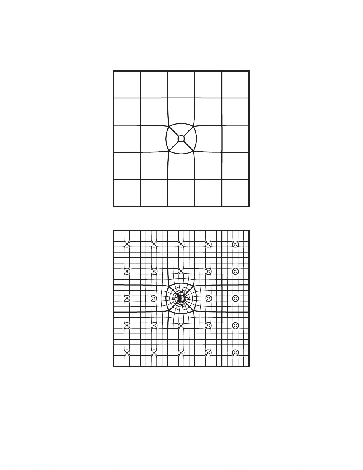
TRANSACTIONS OF THE AMERICAN MA THEMA TICAL SOCIETY V olume 00, N umber 0, Pages 000– 000 S 0002-9947(XX)0000 -0 SNO WBALLS ARE QUASIBALLS DANIEL MEYER Abstract. W e int ro duce snowb al ls , which are compact sets in R 3 homeomor- phic to the unit ball. They ar e 3-dimensional analogs of domains in the plane bounded b y snowﬂak e curv es. F or eac h snowball B a quasiconform al map f : R 3 → R 3 is constructed that maps B to the unit ball. 1. Introduction 1.1. Quasiconformal and quasi symmetric Maps. The Riemann mapping the- orem asserts that co nformal maps in the plane are ubiquitous. Ho wever, in higher dimensions all co nformal maps are M¨ obius transformations (b y a theorem of Liou- ville). The most fruitful generaliza tion of confor malit y is the following. A homeo- morphism f : R n → R n is called quasic onformal if there is a co nstant K < ∞ suc h that for all x ∈ R n , (1.1) K ( x ) := lim ǫ → 0 max | x − a | = ǫ | f ( x ) − f ( a ) | min | x − b | = ǫ | f ( x ) − f ( b ) | ≤ K. F or confor mal maps the above limit is 1 everywhere. A conformal map “maps inﬁnitesimal balls to inﬁnitesimal balls” , while a quasico nformal map f “maps inﬁnitesimal balls to inﬁnitesimal ellipsoids of uniformly b ounded eccentricit y”. Alternatively , at almost every p oint ther e is an inﬁnitesimal ellipsoid that is ma pp ed to an inﬁnitesimal ball by f (the inverse f − 1 is quasiconforma l as well). Thus f assigns an el lipsoid-ﬁeld to the domain. Quasiconformal maps are muc h better understo o d in the plane than in higher dimensions. The reason is that b y the me asur able Ri emann mapping the or em for e very given ellipse- ﬁeld in the plane (with uniformly b ounded eccen tr icit y), we can ﬁnd a quasiconformal map f r e alizing this ellipse-ﬁeld. No such theo r ems exist in higher dimensio ns. The cla s sical refer ence on quasiconforma l maps in R n is [V¨ ai71]. A clo s ely related notion is the following. A homeomorphism f : X → Y o f metric spaces is called quasisymmetric if there is a homeomorphism η : [0 , ∞ ) → [0 , ∞ ) such that | x − a | | x − b | ≤ t ⇒ | f ( x ) − f ( a ) | | f ( x ) − f ( b ) | ≤ η ( t ) , for all x, a , and b , with x 6 = b . Receiv ed by the editors August 16, 2007. 2000 Mathema tics Subje ct Cla ssiﬁc ation. Pr imary: 30C65. Key wo r ds and ph r ases. Quasiconformal maps, quasiconformal unifor mization, snowball. This researc h w as partially supported by an NSF postdo ctoral fell o wship and b y NSF gran t DMS-0244421. c  1997 American Mathematical So ciety 1 2 DANIEL M EYER Quasisymmetry is a global notion, while qua siconformality is an inﬁnitesimal one. Ev ery qua sisymmetry is qua s iconformal (pic k K = η (1)). In fact in R n , n ≥ 2 , the tw o notions coincide. This is actually true for a la rge class of metric spaces; see [HK98]. The classical pap er on qua sisymmetry is [TV80]. A recent exp os ition can be found in [Hei01]. 1.2. Q uasi circles and Quasisph e res. While quasico nformal maps share man y prop erties with co nformal ones, they are not smo oth in g eneral. F or example, one can map the snowﬂake (or v on Ko ch curve) to the unit circle by a quasiconfor mal map (of the plane). In general, we ca ll the image of the unit c ir cle under a q uasi- conformal map of the plane a quasicir cle . Ahlfors’s 3 -p oint c ondition [Ahl63] gives a complete ge ometric character ization: a Jor dan cur ve γ in the plane is a quasicir- cle if and only if for each t w o p oints a, b on γ the (smalle r ) ar c b et ween them has diameter comparable to | a − b | . This condition is easily chec k ed for the snowﬂak e. On the other ha nd, ev e ry quasicir cle can be obtained by an explicit snowﬂake-t ype construction (see [Roh01]). Analogous questions in higher dimensions are m uc h harder. At the moment a cla s siﬁcation of quasispher es / quasib al ls (images of the unit spher e/ball under a quasiconfor mal map of the whole spa c e R 3 ) seems to b e out o f reach. In fac t very few no n-trivial examples of such maps have b een exhibited. Some such maps (in a sligh tly diﬀeren t setting) ca n be found in [V¨ ai99]. First s nowﬂak e-t ype examples were constructed in [Bis99] and [DT99]. These quasispheres do no t c ontain any rectiﬁable curves. That quasisy mmetric embeddings of certain surfa c e s exist seems to follow from ongoing work of Cannon, Floyd, and Parry ([CFP01]), the main to ol used b eing Cannon’s c ombinatorial Riema nn mapp ing the or em [Can9 4]. Thes e surfaces are deﬁned abstractly , so no extension to a n amb ient space (like R 3 ) is po ssible. A diﬀerent (though r elated) approa ch is to use cir cle packings as in [BK02]. The quasispheres considered there a re Ahlf ors 2 -r e gular , so in a s ense are alr eady 2-dimensional. Their result provides one step in the pr o of of Cannon ’s c onje ctur e , which deals with uniformizing (m apping to the unit spher e by a quasisymmetry) top ological spheres app ear ing as the bounda ry at inﬁnity of Gromov h yp erb olic groups. 1.3. R esults and Outli ne. Here we co nsider sn owspher es S which are top o log- ically 2- dimensional ana logs of the snowﬂake, homeo mo rphic to the unit sphere S = { x ∈ R 3 : | x | = 1 } . They are boundaries o f snowb al ls B , which are homeo- morphic to the unit ball B = { x ∈ R 3 : | x | ≤ 1 } . A co mplete deﬁnition is given in Section 2. W e g ive a slightly imprecise description here, av oiding tec hnica lities. Start w ith the unit cub e. Divide each face into N × N squares o f side-leng th 1 / N (called 1 / N - squares). Put cub es of s ide-length 1 / N on s o me 1 / N -squa r es. W e require tha t the sma ll cubes are a dded in a pattern t hat respects the symmetry group of the cub e. This means that o n every side of the unit cub e the pa tter n is the same, as well as that on each side we can rotate and reﬂect without changing the patter n. Figure 1 illustrates one e x ample with N = 7. The b ounda ry of the res ulting doma in is a po lyhedral surface built fr om 1 / N -squar es, called the ﬁrst appr oximation o f the snowspher e . Sub div ide each 1 / N -sq ua re again, and put cube s of side-length 1 / N 2 on them in the same pattern a s b efore. Th us we obtain a domain bounded by a polyhedra l surface built from 1 / N 2 -squares (the se c ond SNOWBALLS ARE QUASIBALLS 3 f Figure 1. E m bedding of the s nowball. appr oximation of the snowspher e ). Iterating t his pr o cess we ge t a snowb al l B as (the closure of ) the limiting do main, with a snowspher e S a s its bo undary . R emarks. One has to imp ose relatively mild conditions to ensure tha t the sno w- sphere S is a top ologica l sphere, i.e., do es not have self-intersections. In every step a diﬀere n t pattern and a diﬀerent num ber N j may b e used. W e then hav e to assume that sup j N j < ∞ . The main theorem we pro v e is the following. Theorem 1. F or every snowb al l B ther e is a quasic onformal map f : R 3 → R 3 that maps B t o the unit b al l B . Obviously then f ( S ) = S . The pro of is broken up into tw o par ts. Theorem 1A. Every snowspher e S c an b e mapp e d to t he un it spher e S by a qua- sisymmetry f : S → S . This theorem will b e pro v ed in Section 3 . W e ﬁr st equip the j -th approxima- tion of the snowsphere with a c onformal s t ructur e in a standa rd wa y . By the uniformization the or em it is conformally equiv a lent to the sphere. The proo f of the quasisymmetry of the ma p f relies ess e ntially on t wo facts. The ﬁrst is that the num ber o f small squares in tersecting in a vertex is b ounded by 6 throughout the whole co nstruction. This means that if one lo oks at a square and adjacent squares, only ﬁnitely ma ny combinatorially diﬀerent situations o ccur. The second ingredient is that c ombinatorial e quivalenc e implies c onformal e quivalenc e . Th us in combinatorially equiv a lent sets the dis tortion is comparable by K o eb e’s the or em . Only ﬁnitely many co nstants appear , one for e a ch of the (ﬁnitely ma n y) combina- torial situa tio ns of s uitable neighbo rho o ds. This idea a lready app ear ed in [Mey 0 2]. The remainder of the pa per co ncerns the extension of the map f to f : R 3 → R 3 . The construction is explicit, tho ugh somewhat technical. In Section 4 some ma ps and extensions that will be useful later on are provided. The snowball is decomp osed in Section 5 in a W hitney-typ e fa s hion, whe r e the size of a piece is compara ble to its distance from the b oundary (the snowsphere). In Section 6 the pieces are mapp ed to the unit ball and reassemb led there . O ne has to make sure that f a grees on 4 DANIEL M EYER int ersecting pieces (is well deﬁned). The explicit construction o f the map f : S → S allows us to co n trol distortion. In Section 7 the remaining part of Theore m 1 is prov e d. Theorem 1B. The map f fr om The or em 1A c an b e extende d to a quasic onformal map f : R 3 → R 3 . Thu s one o btains a larg e cla ss of quasispher es. The Xmas tr e e examp le from [Mey02] shows that ther e a re quasispher e s (in R 3 ) having Hausdo rﬀ dimension arbitrar ily close to 3. O n the other hand, o ne can construct quas ispheres having Hausdorﬀ dimension 2 that are not Ahlfors 2-r egular. 1.4. No tation. b C = C ∪ { ∞} is the Riemann sphere, S = { x ∈ R 3 : | x | = 1 } the unit sphere, B = { x ∈ R 3 : | x | ≤ 1 } the (closed) unit ball, D = { z ∈ C : | z | < 1 } the unit disk. The Euclidean norm in R n is denoted by | x | , the Euclidea n metr ic by | x − y | . The spher e S and the unit ball B are equipped with the Euclidean metric inherited from R 3 , unless otherwise noted. W e iden tify b C with S , meaning b C is equipp ed with the c hordal metr ic. Maximum norm a nd metric are denoted by k x k ∞ and k x − y k ∞ . F or tw o non-ne g ative express io ns f , g w e wr ite f ≍ g if there is a consta n t C ≥ 1 such that 1 C g ≤ f ≤ C g . W e will often re fer to C by C ( ≍ ), for example we will write C ( ≍ ) = C ( n, m ) if C dep ends on n and m . Similarly we write f . g o r g & f for tw o non-negative expressions f , g if there is a constant C > 0 such tha t f ≤ C g . The constant C is r eferred to as C ( . ) or C ( & ). The in terior of a set S is denoted b y in t S , the clo sure b y clos S , while U ǫ ( S ) := { x : dist( x, S ) < ǫ } denotes the op en ǫ -neighb orho o d of a set S . Let d A ( B ) := inf { ǫ : B ⊂ U ǫ ( A ) } (1.2) = sup { dist( b, A ) : b ∈ B } . The Hausdorﬀ distanc e b etw een t w o sets A, B is Hdist( A, B ) := max { d A ( B ) , d B ( A ) } . Lemma 1. 1 . L et A, B , C b e arbitr ary sets; then Hdist( A, B ) ≤ Hdist( A, C ) + Hdist( C, B ) , (1.3) dist( A, B ) ≥ dist( A, C ) − d C ( B ) (1.4) ≥ dist( A, C ) − Hdist( C, B ) . (1.5) Pr o of. The ﬁrst inequa lit y is clear. T o see the se cond inequality , let b ∈ B b e a rbitrary ; then dist( A, C ) = inf a ∈ A c ∈ C | a − c | ≤ inf a ∈ A | a − b | + inf c ∈ C | b − c | = inf a ∈ A | a − b | + dist ( b, C ) ≤ inf a ∈ A | a − b | + d C ( B ) . T aking the inﬁmu m with resp ect to b ∈ B yields (1.4). The la s t inequality follo ws from d A ( B ) ≤ Hdist( A, B ).  SNOWBALLS ARE QUASIBALLS 5 W e identify R 2 with the xy -plane in R 3 ; s imilarly when wr iting “[0 , 1 ] 2 ⊂ R 3 ”, we identify [0 , 1] 2 with [0 , 1] 2 × { 0 } , etc. 1.5. Polyhedral Surfaces. Snowspheres will b e approximated by p olyhedr al sur- faces. W e rec a ll some well-known facts. Let S ⊂ R 3 be a p olyhedral s ur face homeomorphic to the sphere S . The following is Theorem 17.12 in [Moi77]. Theorem (PL-Sch¨ onﬂies Theorem for R 3 ) . Ther e is a PL-(pie c ewise line ar) home- omorphism h : R 3 → R 3 such that h ( ∂ [0 , 1] 3 ) = S . Corollary 1.2. L et S b e a p olyhe dr al surfac e home omorphi c to S . Then the cl osur e of the b ounde d c omp onent of R 3 \ S is bi-Lipschitz e quivalent to the cub e [0 , 1] 3 . 2. Snowballs and Snowspheres 2.1. Gene rators. W e ﬁr st in tro duce some ter minology . By the pyr amid ab ove (denoted by P + ) the unit square [0 , 1] 2 ⊂ R 2 ⊂ R 3 we mean the p yramid with base [0 , 1] 2 and tip ( 1 2 , 1 2 , 1 2 ) (which is the center of the unit cub e [0 , 1 ] 3 ). The pyr amid b elow the unit square is the one with base [0 , 1] 2 and tip ( 1 2 , 1 2 , − 1 2 ). W e denote by P the double p yr amid o f the unit squar e, which is the union of the tw o pyramids deﬁned ab ov e. The double pyramid P ( Q ) o f a n y sq ua re Q ⊂ R 3 is deﬁned as the image of the double pyramid P under a similar it y (of R 3 ) that maps the unit squar e to Q . If we g ive Q an or ien tation w e also speak of its p yramids ab ove and b elow . Consider tw o distinct unit square s in the grid Z 3 . Their double p yramids in ter- sect at most in a (common) face, which means they ha v e disjoin t interiors. An N - gener ator (for an integer N ≥ 2) is a p olyhedra l surface G ⊂ R 3 built from squares of side-length 1 N = δ ( δ - squ ar es ). W e require: (i) G is homeomor phic to the unit square [0 , 1] 2 . (ii) The boundary of G (as a s urface) consists of the fo ur sides of th e unit square: ∂ G = ∂ [0 , 1] 2 . (iii) G is contained in the double p yramid P and intersects its b oundar y only in the bo undary (the four edges) of the unit squar e: G ⊂ P and G ∩ ∂ P = ∂ [0 , 1] 2 . (iv) The angle be t w een tw o adjacent δ -s q uares is a m ultiple of π 2 (so it is π 2 , π , or 3 π 2 ). (v) The genera tor G is symmetric , meaning it is inv a riant under orientation pre- serving symmetries of the unit squa re [0 , 1 ] 2 ; more precisely under rotations by m ultiples of π / 2 around the axis { ( 1 2 , 1 2 , z ) } , and reﬂections on the pla nes { x = 1 2 } , { y = 1 2 } , { x = y } , and { y = 1 − x } . Deﬁnition 2.1. W e say a surface that can b e decomp osed into squares having edges in a grid δ Z 3 lives in the g rid δ Z 3 . Similarly , w e say a domain lives in a grid δ Z 3 if this is true for its b oundary . So an N -ge nerator lives in the g rid 1 N Z 3 . F or a given N there can b e only ﬁnitely many s uch generators . One last ass umption abo ut generator s will be made, though it is not s trictly necessary . Ho wever, it will simplify the decomp osition o f the sno wball B in Sec tio n 5 considerably . W e do not allow the situation indica ted in Figur e 2 to o ccur . T o be more precise consider a n int erior vertex of G , meaning a po in t v ∈ ( G ∩ δ Z 3 ) \ ∂ [0 , 1] 2 . 6 DANIEL M EYER Figure 2. The forbidden co nﬁguration. A t v it is po s sible that 3 , 4 , 5 or 6 δ -squares in tersect. W e do not allow 6 δ -squares around v which for m successive ang le s of π , 3 2 π , π / 2 , π , 3 2 π , π / 2 . All o ther (allow ed) po ssibilities (up to rotations/reﬂections ) of how δ -squares may intersect in a vertex are indicated in Figure 10. (vi) The generator G do es not contain a forbidden c onﬁgu r ation as in Figur e 2. In the nex t s ection we will deﬁne the appr oximations S j of the snowsphere, which will be built successively from generators. R emarks. • Condition (i) in the deﬁnition of a gener a tor is clearly necessary for S j to be homeomorphic to the sphere S . • Condition (ii) enables us to replace the δ j -squares b y a scaled copy of a generator . • The third co ndition (iii) g uarantees that the approximations S j (and ulti- mately the s nowsphere S ) are top o logical spheres. See the next subsection. • The fourth c ondition (iv) is equiv ale nt to saying that a gener a tor lives in the grid 1 N Z 3 . It is most likely sup erﬂuous. How ever, we w ere not able to ﬁnd a convincing argumen t for this. • The ﬁfth condition (v) is necessa ry for our metho d to work. Av oiding it would b e v er y de s irable. Indeed, tackling the non-symmetric case might b e the ﬁrst step tow ards a general th eory . • The last condition is impo sed to a v oid more technicalities when deco mpo s- ing the snowball in Section 5.2. See the Remark on page 31. 2.2. Approximations of the Snowsphere. A snowb al l B is a three-dimensional analog o f the domain bo unded by the snowﬂake curve. It is a compa ct set in R 3 homeomorphic to the closed unit ball B = { x ∈ R 3 : | x | ≤ 1 } . The co rresp onding snowspher e S := ∂ B is homeomorphic to the unit spher e S = { x ∈ R 3 : | x | = 1 } = SNOWBALLS ARE QUASIBALLS 7 ∂ B . W e will obtain S as the Hausdorﬀ limit of appr oximations S j . T o obtain S j +1 from S j we re place small squares b y scaled generator s. The 0 -th appr oximation of the sn owspher e S 0 is the surface o f the unit cub e, S 0 := ∂ [0 , 1] 3 . Now replace each of the six faces of S 0 by a rotated copy of an N 1 - generator to get S 1 , the ﬁrst appr ox imation of the snowspher e . It is a p olyhedral surface built from 1 N 1 -squares . W e construct S 2 by replacing eac h 1 N 1 -square of S 1 by a sc aled (by the factor 1 N 1 ) and rotated copy of an N 2 -generato r. Inductively the j -th appr oximations of the snowspher e S j are constructed. E ach S j is a polyhe dr al surface built from squares of side-leng th (2.1) δ j := 1 N 1 × · · · × 1 N j . It will b e conv enient to set δ 0 := 1 and δ ∞ := 0. Note that when construct- ing S j +1 from S j each δ j -square is replaced by the same N j +1 -generato r. W e do how e ver allo w t w o δ j -squares Q 1 and Q 2 to b e repla c ed b y scaled copies of the N j +1 -generato r with diﬀer en t orientation . So the generator can “stic k out” on o ne square and “p oint inw ar ds” on another. In each step a diﬀerent generator may be used. W e do r equire that (2.2) N max := max j N j < ∞ . This implies tha t only ﬁnitely many diﬀerent generators are used. The constructio n may b e pa raphrase d a s follows. Pick a ﬁnite set of gener ators. In each step pic k a generator from this set to construct the next approximation. All relev a n t constants will dep e nd on N max only . Such a constant is called uniform . Lemma 2. 2 . The appr oximations S j ar e t op olo gic al spher es. Pr o of. Let g 0 : S → S 0 = ∂ [0 , 1] 3 be a homeomor phism. F or every N j +1 -generato r G j +1 we ca n ﬁnd a homeo mo rphism [0 , 1] 2 → G j +1 which is cons ta n t o n ∂ [0 , 1 ] 2 . Apply this homeomor phism to every δ j -square in S j to get a contin uous and sur- jective map g j +1 : S j → S j +1 , which is constan t on the 1-skeleton of S j (edges of δ j -squares in S j ). T o se e in- jectivit y consider t wo distinct δ j -squares Q , Q ′ ⊂ S j . Then G := g j +1 ( Q ) , G ′ := g j +1 ( Q ′ ) ⊂ S j +1 are scale d (by δ j ) co pies of the N j +1 -generato r. Note that they are co ntained in the double pyramids, G ⊂ P ( Q ) , G ′ ⊂ P ( Q ′ ). By condition (iii) of generator s g j +1 (in t Q ) = int G ⊂ int P ( Q ) and g j +1 (in t Q ′ ) ⊂ int P ( Q ′ ) . Thu s g j +1 (in t Q ) ∩ g j +1 (in t Q ′ ) = int P ( Q ) ∩ in t P ( Q ′ ) = ∅ . Note also that int P ( Q ) do es not intersect the 1-skeleton of S j . Thu s g j +1 is injective, hence a homeo- morphism. This s hows by induction that e very approximation S j is a top olo gical sphere.  The appr oximations S j are p olyhedral surfaces. Thus R 3 \ S j has tw o comp onents by the P L -Sch¨ onﬂies theorem. 8 DANIEL M EYER (a) Generator wi th enclosing pyramid. (b) Pyramids on each 1 N 1 -square. Figure 3. Gener ator and p yramids in the grid 1 N 1 Z 3 . Call the edges/vertices of a δ j -square in S j δ j -e dges/vertic es . Then the approxi- mations S j form a c el l c omplex in a natura l wa y . Na mely the δ j -squares /edges/ver- tices in S j , are the 2-, 1-, and 0-cells . 2.3. Snowspheres. Note that Hdist ( S j , S j +1 ) ≤ δ j ≤ 2 − j . Thus we can deﬁne the sno wsphere S as the limit of the approximations S j in the Hausdorﬀ topo logy . It is possible to prov e that S is a topolo gical sphere as in Lemma 2.2. How ever we would hav e to make a dditional assumptions o n the maps g j . Therefore we p ostp one the pro of that S is homeo mo rphic to S un til Corollar y 3.1 1. W e call the closure o f the b ounded comp onents of R 3 \ S the snowb al l B . It will follo w from Theorem 1 B that B is homeomorphic to a closed ball. S ee also Corollar y 5 .4. When a snowsphere S is given, “ N j -generato r” will alw a ys refer to the one used in the j - th step of the construction. It will often be conv enien t to consider o nly one “face” T o f the snowsphere, i.e., the part of it that was constructed from o ne of the s ides of the s urface of the unit cube . Mo re precisely let T 0 = [0 , 1] 2 be the unit square, T 1 be the N 1 -generato r, T 2 the surface obtained by re pla cing each 1 N 1 -square by a scaled copy o f the N 2 - generator , and s o on. Then T := lim j T j in the Hausdorﬀ top ology . Consider the N 1 -generato r (= T 1 ) a nd its enclo sing double pyramid P . Figure 3(a) sho ws a 2-dimensio nal pictur e wher e w e cut through the middle (along the plane y = 1 2 ). Only the upper pyramid is depic ted. F or con v enience the picture also indicates the g rid 1 N 1 Z 3 (or r ather its 2-dimensional intersection 1 N 1 Z 2 ). W e note that • the height of T 1 is at most 1 2 − 3 2 1 N 1 . Here the pre c is e meaning of “ height” is the max ima l distance of a po in t in the generator from the base s quare [0 , 1] 2 . This is easily seen fro m Figure 3(a). Indeed, the next lay er of 1 N 1 -cub es (having height 1 2 − 1 2 N 1 ) would intersect the b oundar y of the double pyramid (or lie o utside). If N 1 is even the height is at most 1 2 − 2 N 1 . The pro jection of any genera tor to the xy -pla ne is the square [0 , 1] 2 . Thus we note the following consequence o f the ab ov e: (2.3) Hdist ∞ ( S j , S j +1 ) ≤ Hdist( S j , S j +1 ) ≤  1 2 − 3 2 1 N j +1  δ j . SNOWBALLS ARE QUASIBALLS 9 Here “Hdist ∞ ” is the Hausdorﬀ distance taken with re s pec t to the maximum metric; see Subsection 5.2. Put pyramids on the 1 N 1 -squares of T 1 . These stay inside t he double p yramid P ; see Figure 3(b). Consider the pyramids of interior 1 N 1 -squar es , i.e., square s that do not in ter sect the bo unda ry of the unit square ∂ [0 , 1] 2 . These ha v e distance at least √ 2 2 1 N 1 from the surface of the enclosing double pyramid P . If w e no w replace eac h 1 N 1 -square b y the N 2 -generato r to get T 2 , we see that T 2 stays inside the 1 N 1 -pyramids depicted in Figure 3(b) . Induction yields that a ll T j and hence T are contained in the double pyramid P . F urthermore, if Q j is an int erior δ j -square of T j , then the double p yramid of Q j has dis tance √ 2 δ j / 2 from the bo undary ∂ P . W e co nclude • T is contained in the do uble pyramid P and intersects its b ounda ry o nly in the b oundary of the unit squa r e: T ⊂ P a nd T ∩ ∂ P = ∂ [0 , 1] 2 . • The height o f T is at most 1 2 − 1 N 1 ≤ 1 2 − 1 N max . ( ∗ ) Again b y “he ig ht ” we mean the maximal distance of a point in T fr o m the bas e square [0 , 1] 2 . The pr o jection of T to the xy -pla ne is still the sq ua re [0 , 1] 2 . Thus we co nc lude by ( ∗ ) above that the Hausdor ﬀ distance betw een S j and S s atisﬁes (2.4) Hdist( S j , S ) ≤ δ j  1 2 − 1 N max  . Recall that the j -th approximation of the snowsphere S j was built fro m δ j - squares. The part of the snowsphere whic h was c o nstructed by replacing one such δ j -square Q ⊂ S j (inﬁnitely often) b y generators is called a cylinder o f or der j (or j -cylinder ). By the pre v ious argument this cylinder is contained in the double pyramid P ( Q ) of Q , so w e can deﬁne more precisely X j = X j ( Q ) := P ( Q ) ∩ S to b e the j -cylinder with b ase Q . The set of al l j -cylinders is denoted b y X j . It will be co n venien t to let S b e the (o nly) − 1-cylinder . Set δ − 1 := 2 so that diam X j ≤ √ 2 δ j , for every j -cylinder X j . F or every p oint x ∈ S there is a (not necessarily unique) s e quence ( X j ) j ∈ N , where X j is a j -cylinder such tha t (2.5) X 0 ⊃ X 1 ⊃ X 2 ⊃ · · · ⊃ \ j X j = { x } . If we use the same generator with the same orientation throughout the construc- tion of S , we get a self-similar snowspher e . In that ca se ea ch cylinder is a (scale d and rotated) copy o f T . Now consider a δ j -square Q ⊂ S j , its double p yr amid P ( Q ), and its cylinder X j = X j ( Q ). Then X j is co n tained in P ( Q ) and intersects it only in t he boundary of Q b y the same reasoning as above: X j ∩ P ( Q ) = ∂ Q. 10 DANIEL M EYER Now let R ⊂ S j be a second δ j -square. Their do uble pyramids P ( Q ) and P ( R ) int ersect only at the boundar y : P ( Q ) ∩ P ( R ) = ∂ P ( Q ) ∩ ∂ P ( R ) (they have disjoint int erior). It follows that the cy linder s X j ( Q ) ⊂ P ( Q ) and X j ( R ) ⊂ P ( R ) in tersect only in the intersection o f Q and R : X j ( Q ) ∩ X j ( R ) = Q ∩ R . Thu s t w o distinct no n-disjoint j -cylinders can intersect in an edge or a vertex (contained in δ j Z 3 ). Hence the j -cylinders form a cell complex in a natura l w ay . Lemma 2.3. The set of δ j -squar es in the appr oximations S j is c ombinatoria l ly e quivalent to the set of j -cylinders. Mor e pr e cisely map e ach δ j -e dge/vertex to itself and e ach δ j -squar e Q ⊂ S j to its cylinder X j ( Q ) ∈ X j , Q 7→ X j ( Q ) . This map is a c el l c omplex isomorphism. 2.4. Co mbinatorial Di stance on S . As a s ubset of R 3 , the snowsphere S inherits the Euclidean metric tha t we deno te by | x − y | . O ften it will b e convenien t to describ e distances in purely combinatorial terms. Giv en points x, y ∈ S le t (2.6) j ( x, y ) := min { j : there exist disjoin t j -cylinders X j ∋ x, Y j ∋ y } . One may view S as the Gromov-Hausdor ﬀ limit of j -cylinder s. The j = j ( x, y )-th approximation S j is the ﬁrst in which it is possible to distinguis h x and y . Lemma 2. 4 . F or al l x, y ∈ S we have (2.7) | x − y | ≍ δ j , wher e j = j ( x, y ) and a c onstant C ( ≍ ) = C ( N max ) . Pr o of. Let x, y ∈ S be arbitrary , and let j := j ( x, y ). Consider ( j − 1)-cy linders X j − 1 ∋ x and Y j − 1 ∋ y . Then X j − 1 ∩ Y j − 1 6 = ∅ , by the deﬁnition of j ( x, y ). Therefore (2.8) | x − y | ≤ diam X j − 1 + diam Y j − 1 = √ 2 δ j − 1 + √ 2 δ j − 1 ≤ 2 √ 2 N max δ j . F or the other inequality let X j ∋ x and Y j ∋ y b e disjoint j -cylinders. Note that t wo disjoint j -cy linders are clos est when their bases are opp osite faces o f a δ j -cub e. Their distance then is at least δ j − 2 δ j  1 2 − 1 N max  = 2 δ j N max , which is the distance of base squares − twice the height of j -cylinders, b y Subsection 2.3. Hence (2.9) | x − y | ≥ dist( X j , Y j ) ≥ 2 δ j N max , which ﬁnishes the pro of.  The last lemma s hows tha t δ ( x, y ) := δ j ( x,y ) is a quasimetric . Howev er δ ( x, y ) will violate the triangle inequality . SNOWBALLS ARE QUASIBALLS 11 2.5. E xampl e. Our main example to illustrate o ur co nstruction will b e the self- similar snowball with generator as illustrated in Figure 4. It is the unit square divided in to 25 1 5 -squares where w e put a 1 5 -cub e onto the middle square. Notation. When r eferring to this par ticular example we will alwa ys use “ b ” , i.e., b S denotes this snowsphere, b S j its j -th approximation, a nd so on. Then b δ j = 5 − j . 3. Uniformizing the Snowsphere 3.1. Introduction. In this sec tio n we map the snowsphere S to the unit sphere S by a quasisymmetry f , i.e., prov e Theor em 1A. W e ca ll f a u niformization of the sno wsphere S . Recall from equation (2.5) that for ev ery point x ∈ S there is a sequence X 0 ⊃ X 1 ⊃ X 2 ⊃ . . . , X j ∈ X j , suc h that T j X j = { x } . It will therefore be enoug h to map the j -cylinders X j ⊂ S to j - tiles X ′ j ⊂ S , which will again satisfy X ′ 0 ⊃ X ′ 1 ⊃ X ′ 2 ⊃ . . . . “Cylinders” live in the s nowsphere S and “tiles” on the unit spher e S . Generally ob jects in S will b e denoted with a “prime” ( X ′ , x ′ , and so on), to distinguish them from ob jects in the s nowsphere S and its a pproximations S j . W e will then de ﬁne (3.1) f ( x ) = x ′ , where { x ′ } = \ j X ′ j . The decomp osition of the unit sphere S in to j -tiles X ′ j is done by using the uni- formization of the j -th approximation of the snowsphere S j . The proof that the map f is a quasisymmetry relies on t wo facts. Firs t, a t mo st 6 j -cylinder s (and thus j -tiles) can in tersect in a common v ertex. Second, t w o s ets of j -tiles a nd k -tiles whic h “have the s ame combinatorics” are a ctually c onforma l ly e quivalent . The quasis ymmetry is then essentially an ea s y consequence of the Ko eb e distortion theorem. 3.2. Uniform izing the appro xim ations S j . Consider the j -th appr oximation S j of the snowsphere S . This is a p olyhedr a l s ur face where each face is a δ j -square. W e will view S j as a Riema nn surfac e . T o do this we need c onformal c o or dinates on S j , meaning that changes of coor dinates are conformal maps. 3.2.1. Conformal Co or dinates on the Appr oximations S j . • F or each δ j -square Q the a ﬃne, or ien tation pres erving ma p int Q → int[0 , 1] 2 is a chart. • F or tw o neighb oring δ j -squares P , Q (i.e., ones whic h shar e an edge), the map int ( P ∪ Q ) → int([0 , 2] × [0 , 1]) , Figure 4. Gener ator used for our main example. 12 DANIEL M EYER P S f r a g r e p la c e m e n t s z 7→ z 4 / 3 P S f r a g r e p la c e m e n t s z 7→ z 4 / 3 z 7→ z 4 / 5 Figure 5. Co nformal coo r dinates on a poly he dr al surface. which ma ps P (aﬃnely , o rientation preserving ) to [0 , 1] 2 , Q (a ﬃnely , orien- tation pres e r ving) to [1 , 2] × [0 , 1], and P ∩ Q to { 1 } × [0 , 1], is a chart. Using (hop e fully) in tuitiv e notation we s o metimes write: P ∪ Q may b e mapp e d c onformal ly t o   . So P and Q are c onformal r eﬂe ctions of each other in these co ordina tes . • Consider a vertex v . Let Q 1 , . . . , Q n be the δ j -squares c o nt aining v , labeled with p os itive orientation around v . Map the neighborho o d int( S Q k ) o f v by z 7→ z 4 /n . More precise ly the c hart is co nstructed as follows. Map Q 1 to the unit squa re [0 , 1] 2 as ab ov e with v 7→ 0. The unit s quare [0 , 1] 2 is subsequently mapped by the map z 7→ z 4 /n . Ma p the second δ j -square Q 2 as b efore to [0 , 1] 2 (again with v 7→ 0), which is then mapp ed by z 7→ e 2 π i/n z 4 /n . Alterna tiv ely we could have mapped Q 2 to [ − 1 , 0] × [0 , 1] and subsequently b y the map z 7→ z 4 /n . So the image of Q 2 is a conformal reﬂection of the image of Q 1 , alo ng the s ha red side [0 , e 2 π i/n ]. The third δ j -square Q 3 is mapp ed to [0 , 1] 2 , a nd then by z 7→ e 4 π i/n z 4 /n and so on. Again the image of Q 3 is a reﬂection of the image of Q 2 , analog ously for the other δ j -squares . Since each ma pped δ j -square for ms an angle of 2 π / n at 0, the last matches up with the ﬁrst, meaning they are confor mal reﬂections of each other. It is immediate that changes of co ordinates ar e conforma l. The charts a re illustrated in Figure 5. With these charts each approximation S j of the snowsphere is a compact, simply connected Riemann surface. There fore S j is confor mally equiv a len t to the sphere SNOWBALLS ARE QUASIBALLS 13 b C b y the uniformization the or em . Identify b C with S ⊂ R 3 . It is not yet clear, how e ver, what the relation is betw een uniformizations o f diﬀer e n t a pproximations S j and S k . W e ther e fo re construct t he uniformiza tions of the S j inductively , wher e this will be a pparent. Start with S 0 , whic h is the surface of the unit cub e ∂ [0 , 1] 3 . Equip S 0 with a conformal structure a s ab ove and map it confo r mally to the Riemann sphere b C using the uniformization theorem. The images of the faces of S 0 decomp ose the sphere b C into 0 - tiles . Edges and v ertices of thos e 0-tiles are the images of edges and vertices of t he faces of S 0 . By symmetr y we c a n assume that the vertices o f the 0-tiles form a cube , i.e., all 0-tiles hav e the s ame size. Denote the s et of all suc h 0-tiles b y X ′ 0 . Each tile X ′ ∈ X ′ 0 is c onformal ly a squar e , meaning w e can map it conforma lly to the unit squa re [0 , 1] 2 , where vertices map to vertices. Consider tw o n eighb oring tiles X ′ , Y ′ ∈ X ′ 0 (i.e., which share an edge). By the deﬁnitio n of our charts they are confor ma l reﬂections of each other. So we could sta rt with one tile and get all o ther tiles by re p ea ted r eﬂection a long the edges. Such a tiling is called a conformal tiling. Deﬁnition 3 .1. A c onformal tiling of a domain D ⊂ b C is a deco mpo sition into tiles D = S T , suc h t hat: • Each tile T is a c losed Jordan re g ion, b ounded by ﬁnitely many analytic arcs. Every suc h arc is part of the boundar y of exactly t w o tiles. • Two dis tinct tiles T and e T hav e disjoint in terior, in t T ∩ int e T = ∅ . • Call the endp oints of the a nalytic arcs (from the b o undaries of the tiles) ver- tic es . The tiling forms a c el l c omplex , where the tiles/ana lytics arcs/vertices are the 2- ,1-, a nd 0 -cells. This means in particula r that distinct tiles can only intersect in th e union of several suc h analytic arcs and v ertices. • Two tiles sharing an analytic bo undary arc ( neighb ors ) are confo r mal re - ﬂections along this arc . Conformal tilings are of course pres e rved under conforma l maps. Now consider the N 1 -generato r G 1 as a Riemann surfa ce using c harts as ab ov e. Note that in t G 1 is s imply connected, and has more than tw o b oundary p oints. Thu s int G 1 is conformally equiv a len t to the unit disk D b y the uniformization theorem. Beca use of sy mmetry , we can map G 1 conformally to the unit squar e [0 , 1] 2 (mapping vertices to vertices as usual). Fig ur e 6 shows the uniformization of the generator b G (see Fig ur e 4 ) of the ex a mple b S . The picture w a s o bta ined by div iding the generator along the diago nals into 4 pieces. One such piece (a 7-gon) w as mapp ed to a quar ter of the unit square by a Sch warz-Chris toﬀel map, using T oby Driscoll’s Sch w arz-Chris toﬀel T o olb ox ( http://w ww.ma th.udel.edu/ ∼ driscoll/ softwa re/ ); see [DT02]. Th us this picture (as well as following ones) is co nformally correct, up to n umerical error s. The images o f the δ 1 -squares in G 1 again form a tiling of the unit square [0 , 1] 2 . Map a second copy of the uniformized genera tor to the square [1 , 2] × [0 , 1] (map the tw o tiled squares to   ). The tilings are sy mmetric with resp ect to the line { 1 } × [0 , 1] b ecause of the s ymmetry of the g enerator G 1 . So we get a conformal tiling of   . Convention. When we hav e a confo r mal map from a s q uare to a tile g : [0 , 1] 2 → X ′ we alwa y s assume that it maps vertices onto each other. The same normaliz ation is used when mapping a tile to another X ′ → Y ′ . 14 DANIEL M EYER Figure 6. Unifor mization of the generator b G of the snowsphere b S . Figure 7. 2-tiles of b S . SNOWBALLS ARE QUASIBALLS 15 The uniformized generator G 1 and ea ch 0-tile X ′ 0 are confo rmally equiv alent to a squar e. So we can map the uniformiza tion of G 1 (the unit square tiled b y images of δ 1 -squares ) to X ′ 0 . The images o f the tiles of [0 , 1] 2 under this map ar e c a lled the 1 -tiles X ′ 1 ⊂ b C . W e deno te the set of all 1-tiles by X ′ 1 . 3.2.2. Pr op ert ies of t he Tiling. • Every 1-tile is confo r mally a square, meaning w e can map it to the unit square [0 , 1 ] 2 by a confor mal map (mapping vertices to vertices). • Each 1-tile is con tained in exactly one 0-tile. • Two neighboring 1-tiles X ′ 1 , Y ′ 1 (tiles which sha re an edge) may b e mapped conformally to th e rectang le   . This is clear when X ′ 1 and Y ′ 2 are con- tained in the same 0-tile X ′ 0 . Assume they are contained in diﬀerent 0-tiles, X ′ 1 ⊂ X ′ 0 ∈ X ′ 0 and Y ′ 1 ⊂ Y ′ 0 ∈ X ′ 0 . Then X ′ 0 ∪ Y ′ 0 can be mappe d conformally to the rectang le   . In this chart the tiles in the left and r ight squa re are symmetric with resp ect to the line { 1 } × [0 , 1]. So X ′ 1 and Y ′ 1 are confor mal r e ﬂections of each o ther. • The set X ′ 1 forms a conformal tiling of the sphere b C . • Each δ 1 -square Q ∈ S 1 is mapp ed to a 1 - tile. Squar es which sha r e a (vertex, edge) are mapp ed to 1-tiles which share a (v ertex, edge) under this map. • The tiling X ′ 1 is a uniformization of the approximation S 1 of the snowsphere. By this we mean the following. Ma p a δ 1 -square Q to its corresp onding 1- tile X ′ by the Riemann map (normalize d by mapping cor resp onding vertices onto eac h other). By reﬂectio n this extends to a neighbor ing δ 1 -square e Q , where it is the Riemann map to the neighbor ing 1- tile e X ′ (again with the “right” normaliza tion a t v e r tices). The map extends to all of S 1 by reﬂection and is well deﬁned. The extensio n is conformal (with resp ect to the conformal structure on S 1 as describ ed ab ov e). The ab ov e procedur e is now iter a ted. Let the j -th tiling of the sphere b C b e given, and let the set of j -tiles be denoted by X ′ j . W e ma p the uniformized N j +1 -generato r to each j -tile X ′ j ∈ X ′ j to get the ( j + 1)-tiles X ′ j +1 ∈ X ′ j +1 . Tiles ar e alwa ys compact. All the above statements ho ld (where 0 is repla ced b y j and 1 by j + 1). Figure 7 shows the 2 -tiles for the example b S . It will b e convenien t to ca ll the whole sphere S the (only) − 1-tile. Let us recor d the prop erties of the tilings. Lemma 3. 2 . The tiles satisfy the fol lowing: (1) Each j -tile is c onfo rmal ly a squar e, me aning we c an map it c onformally to the squar e (mapping vertic es t o vertic es). (2) The set of j -tiles forms a c onforma l t iling for every j ≥ 0 . (3) The j -th tili ng is a uniformizatio n of the appr oximation S j . This me ans ther e ar e c onformal maps (with r esp e ct to the structur e fr om Subse ction 3.2.1) F j : S j → b C = S , such that F j ( Q ) ∈ X ′ j for every δ j -squar e Q ⊂ S j . (4) The ( j + 1) -th tiling sub divides the j -th tiling. This me ans that fo r e ach ( j + 1) -tile X ′ j +1 ther e exists exactly one j -tile X ′ j ⊃ X ′ j +1 . (5) Cal l the images of δ j -e dges/vertic es under the map F j ab ove j -edg e s/vertices . View the j -th tiling as a c el l c omple x ( j -tiles/e dges/ vertic es ar e the 2 -, 1 -, 16 DANIEL M EYER and 0 -c el ls). Then the j -th tiling, t he appr oximation S j , and t he set of j -cylinders ar e c ombinatorially e quivalent by L emma 2.3. (6) Inclusions o f t iles and cylinde rs ar e pr eserve d. This me ans the fol lowing. Consider a δ j -squar e Q j ⊂ S j and a δ k -squar e Q k ⊂ S k . L et X j = X j ( Q j ) ∈ X j , X k = X k ( Q k ) ∈ X k , and X ′ j = F j ( Q j ) ∈ X ′ j , X ′ k = F k ( Q k ) ∈ X ′ k b e the c orr esp onding cylinders (in S ) and tiles (in S ). Then X j ⊂ X k ⇔ X ′ j ⊂ X ′ k . A neighb or o f a j -tile X ′ j is a j -tile Y ′ j which shar es an edge with X ′ j . 3.3. Co ns truction of the Map f : S → S . Reca ll that for any x ∈ S ther e is a sequence (3.2) X 0 ⊃ X 1 ⊃ X 2 . . . , X j ∈ X j , \ X j = { x } . Consider the tiles X ′ j := F j ( X j ), where F j are the ma ps from Lemma 3.2 (3). They satisfy by Lemma 3.2 (6) X ′ 0 ⊃ X ′ 1 ⊃ X ′ 2 . . . . Lemma 3. 3 . The tiles shrink to a p oint, diam X ′ j → 0 , as j → ∞ . In fact diam X ′ j . λ j , for a (un iform) c onstant λ < 1 (and a uniform c onst ant C ( . ) ). W e p ostp one the pr o of until the next subsectio n. By the previo us lemma w e can now deﬁne f : S → S b y (3.3) f ( x ) = x ′ , where { x ′ } = \ j X ′ j . Lemma 3. 4 . The map f is wel l deﬁne d. Pr o of. Given x ∈ S let the sequence ( X j ) j ∈ N be as in (3.2). Assume now that there is a second sequence Y 0 ⊃ Y 1 ⊃ . . . , Y j ∈ X j , satisfying T Y j = { x } . Then ( X 0 ∩ Y 0 ) ⊃ ( X 1 ∩ Y 1 ) ⊃ . . . , where each X j ∩ Y j is compa c t a nd non-empty . Let X ′ j := F j ( X j ), Y ′ j := F j ( Y j ), and { y ′ } := T Y ′ j . By Lemma 3.2 (5) and (6) ( X ′ 0 ∩ Y ′ 0 ) ⊃ ( X ′ 1 ∩ Y ′ 1 ) ⊃ . . . , where each X ′ j ∩ Y ′ j is compact and non-empty . Thus ∅ 6 = \ ( X ′ j ∩ Y ′ j ) ⊂ \ Y ′ j = { y ′ } and ∅ 6 = \ ( X ′ j ∩ Y ′ j ) ⊂ \ X ′ j = { x ′ } . Thu s x ′ = y ′ .  SNOWBALLS ARE QUASIBALLS 17 3.4. Co mbinatorial Equiv alence and Fini teness. The idea s in this subsection should b e considered the “ guts” of the pr o of of Theorem 1 A. Let v b e a vertex of a j -tile; the j -de gr e e of v is the num b er o f j -tiles containing v : (3.4) deg j ( v ) := # { X ′ ∈ X ′ j : v ∈ X ′ } . Consider j -edges and j -tiles of S j containing v . Note that each such j -edge is incident to tw o j -tiles, and ea ch such j -tile is incident to t wo j -edges. So the nu m ber of j -tiles containing v is eq ual to the num ber of j -edg es containing v . In the grid Z 3 there are 6 edges that in tersect at each vertex. Thus the degr ee of vertices is uniformly bo unded, namely (3.5) deg j ( v ) ≤ 6 , for all vertices v and num b ers j . Now co nsider a set of j -tiles (3.6) X ′ = { X ′ 1 , . . . , X ′ n } , where X ′ 1 , . . . , X ′ n ∈ X ′ j . As b efore view X ′ as a c el l c omplex Σ( X ′ ), where j -tiles, j -edges , and j -vertices in S X ′ are the 2-, 1-, and 0-cells of the cell complex. A sec ond set of k -tiles (3.7) Y ′ = { Y ′ 1 , . . . , Y ′ n } , where Y ′ 1 , . . . , Y ′ n ∈ Y ′ k , is said to b e c ombinatorially e quivalent to X ′ , if they are equiv alent w he n viewed as cell complexes. More precisely , there is a cell complex isomor phism (3.8) Φ : Σ( X ′ ) → Σ( Y ′ ) , which is orie n tation preserving . The equiv alence class o f combinatorially equiv ale n t sets of tiles is called the c ombinatorial typ e of X ′ . Otherwise X ′ and Y ′ are called c ombinatorial ly diﬀer ent . Combinatorial equiv alence implies conforma l eq uiv alence. Lemma 3. 5. L et X ′ and Y ′ as ab ove b e c ombinatoria l ly e quivalent. Then ther e is a c onformal map g = g X ′ , Y ′ : int [ X ′ → int [ Y ′ , which maps j -(tiles, e dges, vertic es) to k - (tiles, e dges, vertic es). Pr o of. Let Φ be the c ell complex isomo rphism in (3.8). Without lo ss of generality assume that Φ( X ′ i ) = Y ′ i , for i = 1 , . . . , n . Let g : int X ′ i → int Y ′ i be the co nfo r mal map, normalized by mapping each vertex v ∈ X ′ i to the vertex Φ( v ) ∈ Y ′ i . Neigh- bo ring tiles (in X ′ and Y ′ ) are the conformal image of   . Thu s if X ′ i , X ′ l are neighbors, g extends c o nformally to int( X ′ i ∩ X ′ l ). Interior vertices ar e remov able singularities.  The next lemma shows how one can use the tiling to deﬁne holomor phic maps of the for m z 7→ z n . It will b e a pplied to a co v ering of our c o nformal tilings. Recall that a c onformal tiling may be viewed as a cell co mplex , where the 1-ce lls are the (analytic) bo undary arcs of the tiles. Lemma 3.6. L et V = S { X ′ ∈ X ′ } and W = S { Y ′ ∈ Y ′ } b e two c onformal tilings, wher e e ach t ile is a c onformal squar e. L et v ∈ V and w ∈ W b e vertic es, su ch that the de gr e e at v (nu mb er of tiles interse cting in v ) is a mu lt iple of the de gr e e at w , deg( v ) = n deg( w ) , 18 DANIEL M EYER for some n ∈ N . L et U ( v ) := [ { X ′ ∈ X ′ : v ∈ X ′ } \ [ { 1 -c el ls of V n ot c ontaining v } and U ( w ) := [ { Y ′ ∈ Y ′ : w ∈ Y ′ } \ [ { 1 -c el ls of W not c ontaining w } b e neighb orho o ds of v and w . Then ther e is an analytic map U ( v ) → U ( w ) mapping j -t iles to k -tiles, which is c onformal ly c onjugate to z 7→ z n . Pr o of. La b el the tiles around v by X ′ 1 , . . . , X ′ nm , and the t iles a round w by Y ′ 1 , . . . , Y ′ m po sitively aro und the v ertices. Map the ﬁrst tile X ′ 1 conformally to Y ′ 1 , suc h that v is mapp ed to w . By reﬂectio n this extends conformally to map X ′ 2 to Y ′ 2 . Contin uing to ex tend the map in this fashion X ′ nm gets mapped to Y ′ m . Again this extends b y reﬂection to a c o nformal ma p from X ′ 1 to Y ′ 1 , agree ing with the prev ious deﬁnition of the ma p on X ′ 1 . By changing co or dinates we can write the map in the form z 7→ z n .  Pr o of of L emm a 3.3. One way to prove the lemma would b e to use the rational maps that can b e constructed as in [Mey02]. Since it is well known that the o ccur - ring p ost critic al ly ﬁnite rational maps a re sub-hyp erb olic , the statement is true in the orbifold m etric (see [CG93] and [Mil99]). W e give a self-contained proo f here. The following ma y in fact be vie wed as an e x plicit construction of the or bifold metric. It was s omewhat ins pired by a conv ersation with W. Floyd and W. Parry . Consider ﬁrst a uniformized generator as in Fig ure 6 . The conformal ma ps g from the unit square to a tile are con tractions in the hyper bo lic metric d h ( x, y ) of int[0 , 1] 2 by the Sch w arz-Pick lemma; they are strict c ontr actions for compact subsets of int[0 , 1] 2 . W e wan t to consider a neighborho o d U of the unit square [0 , 1 ] 2 so that we ca n extend the maps g : [0 , 1 ] 2 → tile to U . By Sch w arz-Pick the map g will then b e strictly contracting on the co mpact set [0 , 1] 2 ⊂ U in the hyperb olic metric of U . Let the n umber M ∈ N be the lea st common multiple of all o ccurring degree s deg j ( v ) (recall that this was the n um ber o f j -tiles intersecting in a vertex v ). It is well known that the hyperb olic plane ca n b e tiled with hyperb olic sq uares with angles 2 π/ M if M ≥ 5 (see [Ca r54], sections 398 –400). Alternatively one ma y co n- struct a c ell complex co nsisting of s quares wher e a t ea ch vertex M squares in tersect, put a conforma l structure on the complex (as in Subsection 3 .2 .1), and inv o ke the uniformization theorem (it is not har d to show that the typ e will b e hyperb olic). Let Q b e one hype r b o lic squa re o f the tiling, a nd U b e the neighborho o d co nsist- ing o f a ll hyperb olic squar es with non-empty intersection with Q . The hyperb olic squares in U form a conformal tiling. E a ch vertex of Q belongs to M tiles. Now consider a uniformized generator, whic h is a conforma l tiling of the unit square [0 , 1] 2 as in Figur e 6. Map th is tiling by co nformal ma ps to each hyperb olic square in U . Images of the tiles of [0 , 1] 2 under these ma ps will be denoted by T . The tiles T are again a conformal tiling of U . Let g T be a conformal map from the hyperb olic square Q to such a tile, (3.9) g T : Q → T ( Q. SNOWBALLS ARE QUASIBALLS 19 By the pr e vious lemma g T extends to U a nalytically , g T : U → U . Since Q is compactly contained in U , the map g T is strictly co n tracting on Q in the hyper b o lic metric d U of U (by Sch w arz-Pick, se e for exa mple [Ahl73]): d U ( g ( x T ) , g ( y T )) ≤ λ T d U ( x, y ) , where λ T < 1 for all x, y ∈ Q. Since there a re only ﬁnitely many diﬀeren t g enerators (each with ﬁnitely many squares/ tiles), all t hese maps are contracting w ith a uniform constant λ < 1 . Consider a 0-tile X ′ 0 ∈ X ′ 0 . Let V b e the neighbor ho o d of all 0- tiles having non-empty in tersection with X ′ 0 . As b efor e we can e xtend the confor mal map h : Q → X ′ 0 to an ana ly tic map h : U → V . Since X ′ 0 is compactly co nt ained in V , and b y Sc h w arz-Pick, | h ( x ) − h ( y ) | ≍ d V ( h ( x ) , h ( y )) ≤ d U ( x, y ) , for all x, y ∈ Q, where d V denotes the hyperb olic metric of V . Now consider a j -tile X ′ j ⊂ X ′ j − 1 ⊂ · · · ⊂ X ′ 0 , wher e X ′ k ∈ X ′ k for 0 ≤ k ≤ j . Let Y ′ k := h − 1 ( X ′ k ) ⊂ Q b e their pr e ima ges. Set T 1 := Y ′ 1 . Since Y ′ 2 ⊂ T 1 , we can let T 2 := g − 1 T 1 ( Y ′ 2 ); the map g T 1 is the one from (3.9). Deﬁne inductively T k := g − 1 T k − 1 ◦ · · · ◦ g − 1 T 1 ( Y ′ k ) , for 1 ≤ k ≤ j . Note that Y ′ k ⊂ T 1 , g − 1 T 1 ( Y ′ k ) ⊂ T 2 , g − 1 T 2 ◦ g − 1 T 1 ( Y ′ k ) ⊂ T 3 , and so on. Thu s T k is w ell deﬁned. Note a ls o that T k is one o f the (ﬁnitely many) tiles as abov e. This is seen a s follows. Consider all k -tiles e X ′ k ⊂ X ′ k − 1 and the corr esp onding s ets e Y ′ k , e T k . Then the sets e T k ⊂ Q are the conformal image of the tiling of [0 , 1] 2 obtained as the uniformization of the N k -generato r. The n g T 1 ◦ · · · ◦ g T j ( Q ) = g T 1 ◦ · · · ◦ g T j − 1 ( T j ) = Y ′ j . F or x ′ = h ( x ) , y ′ = h ( y ) ∈ X ′ j , where x, y ∈ Y ′ j ⊂ Q , we ha ve by the above | x ′ − y ′ | . d U ( x, y ) . λ j . The result follows.  3.5. Co mbinatorial Distance on S . Reca ll how j ( x, y ) was deﬁned in (2.6) b y the com bina torics of cylinders (of the s nowsphere). Since tiles (of the sphere) hav e the same combinatorics, we write j ( x ′ , y ′ ) = j ( x, y ) , where x ′ = f ( x ) , y ′ = f ( y ). The pro of of Theor em 1A follows essentially fro m the next tw o lemmas . The ﬁrst concerns int erse cting j -tiles, th us the case j < j ( x ′ , y ′ ); see (2 .6). In the second w e consider disjoint j -tiles, thus the case j ≥ j ( x ′ , y ′ ). The pro o fs ar e essentially the same. In e ach case one ha s to co n trol only ﬁnitely ma n y combinatorial types b y (3.5). Since combinatorial eq uiv alence implies conforma l eq uiv alence by Lemma 3.5, sets o f the same type cannot “lo ok to o diﬀere n t” by the Koe b e distortion theor em. T o paraphrase the main idea of the pr o of, why do constants not blo w up? B e cause there are only ﬁnitely many constant s, one for each com binatorial t ype of suitable neighborho o ds. 20 DANIEL M EYER Lemma 3. 7 . L et X ′ , Y ′ b e j -tiles t hat ar e n ot disjoint. Then diam X ′ ≍ diam Y ′ , with a un iform c onstant C ( ≍ ) . Pr o of. Let X ′ , Y ′ ∈ X ′ j , X ′ ∩ Y ′ 6 = ∅ . Consider the set of tiles Z ′ := { Z ′ ∈ X ′ j : Z ′ ∩ ( X ′ ∪ Y ′ ) 6 = ∅} . There ar e only ﬁnitely man y diﬀerent combinatorial types o f such Z ′ by inequal- it y (3 .5). Th us there ar e only ﬁnitely many diﬀerent conformal types of such Z ′ (b y Lemma 3.5). In gener al S Z ′ is not s imply connected. Fix simply connected op en neighborho o ds U = U Z ′ ⊂ S Z ′ of X ′ ∪ Y ′ , a nd Riemann ma ps h = h Z ′ : D → U with h (0) ∈ X ′ ∩ Y ′ . W e can choose h and U c omp atible with the confor mal equiv- alence. By this we mean that if Z ′ and e Z ′ are combinatorially equiv alen t and g Z ′ , e Z ′ is the map from Lemma 3.5, then U e Z ′ = g Z ′ , e Z ′ U Z ′ , h e Z ′ = g Z ′ , e Z ′ ◦ h Z ′ . Consider preimag e s of X ′ and Y ′ by g in the dis k D ; they are compactly contained. There are only ﬁnitely many diﬀere n t such preima g es, one for ea ch combinatorial t yp e of Z ′ . Thus diam g − 1 ( X ′ ) ≍ diam g − 1 ( Y ′ ) and dist( g − 1 ( X ′ ∪ Y ′ ) , ∂ D ) ≥ ǫ > 0 . Here C ( ≍ ) and ǫ are uniform constants. The s tatement no w follows from Ko eb e’s distortion theorem (see for example [Ahl73]).  Since the n umber of ( j + 1)-tiles that a j -tile co nt ains is unifor mly bounded, one immediately concludes the following corollary . Corollary 3.8. F or any ( j + 1) -tile X ′ j +1 ⊂ X ′ j ∈ X ′ j , we have diam X ′ j +1 ≍ diam X ′ j , wher e C ( ≍ ) is a uniform c onstant. Lemma 3. 9 . L et X ′ , Y ′ b e disjoint j -tiles. Then dist( X ′ , Y ′ ) & diam X ′ , with a un iform c onstant C ( & ) . Pr o of. Cons ider the neigh bor ho o d of j -tiles of X ′ ∈ X j , X ′ := { Z ′ ∈ X ′ j : Z ′ ∩ X ′ 6 = ∅} . The set S X ′ is simply connected. There are only ﬁnitely many diﬀerent combi- natorial types of such X ′ (b y inequality (3.5)). Assume that the tiling o n D induced by the Riemann maps g = g X ′ : D → int S X ′ (with g (0) ∈ X ′ ) dep ends only on the type of X ′ (b y Lemma 3.5). Then dist( g − 1 ( X ′ ) , ∂ D ) ≥ ǫ, where ǫ > 0 is a uniform constant. So b y Ko eb e distortion, dist( X ′ , Y ′ ) ≥ dist( X ′ , ∂ [ X ′ ) ≍ | g ′ X ′ (0) | & diam X ′ .  SNOWBALLS ARE QUASIBALLS 21 The last tw o lemmas enable us to describ e distances in combinatorial ter ms. Lemma 3. 1 0. F or al l x ′ , y ′ ∈ S | x ′ − y ′ | ≍ diam X ′ j , wher e j = j ( x ′ , y ′ ) , x ′ ∈ X ′ j ∈ X ′ j . The c onstant C ( ≍ ) is un iform. Pr o of. Let x ′ , y ′ ∈ S b e a rbitrary , j = j ( x ′ , y ′ ). Then ( j − 1)-tiles X ′ j − 1 ∋ x ′ , Y ′ j − 1 ∋ y ′ are not disjoint. Th us , | x ′ − y ′ | ≤ diam X ′ j − 1 + diam Y ′ j − 1 . diam X ′ j − 1 by Lemma 3.7 . diam X ′ j by Cor ollary 3.8 . On the o ther hand there are disjoint j -tiles X ′ j ∋ x ′ , Y ′ j ∋ y ′ . The r efore by Lemma 3.9, | x ′ − y ′ | ≥ dist( X ′ j , Y ′ j ) & diam X ′ j .  The following is an immediate consequence of Lemma 2.4, Le mma 3 .3, and Lemma 3.10. Corollary 3.11. The map f : S → S i s a home omorphism. In p articular S is a top olo gic al spher e. 3.6. Pro of of Theorem 1A. T o sho w that spaces a re quasisymmetrica lly eq uiv a- lent ca n b e tedious. Therefore o ne often considers the following weak er notion. An embedding f : X → Y o f metric spaces is called we akly quasisymmetric if there is a n um ber H ≥ 1 such that | x − a | ≤ | x − b | ⇒ | f ( x ) − f ( a ) | ≤ H | f ( x ) − f ( b ) | , for all x, a, b ∈ X . Quas isymmetric maps ar e “more nicely” behaved than w eakly quasisymmetric ones. Qua sisymmetry is preserved under comp ositions and inv erses, which do not preserve weak quasisymmetry in general. In many practica lly relev ant cases how ever the t w o no tions coincide. A metric space is called doubling if there is a num ber M (the doubling c onstant ), such that every ball of diameter d can b e cov ered by M sets o f diameter at most d/ 2, for all d > 0. Theorem (see [Hei0 1], 10 .1 9) . A we akly quasisymmetric home omorphism of a c on- ne cte d doubling sp ac e into a doubling sp ac e is quasisymmetric. Obviously S is connected. The snowsphere S (as well as S ) is doubling as a subspace of R 3 . Pr o of of The or em 1A. W e wan t to sho w that the map f : S → S , deﬁned in Subse c tion 3.3, is quasisymmetric. By the ab ove it is enough to s how weak quas isymmetry . Let x, y , z ∈ S , j := j ( x, y ) , k := j ( x, z ) (see (2.6)). Assume | x − y | ≤ | x − z | . 22 DANIEL M EYER Then b y Lemma 2.4 δ j . δ k . (3.10) Let C = C ( . ) = C ( N max ) and choose an integer k 0 = k 0 ( N max ) such that 2 k 0 ≥ C . Then (3.10) implies j ≥ k − k 0 , since N i ≥ 2 for all i . Lemma 3.10 yields | x ′ − y ′ | ≍ diam X ′ j , where x ′ ∈ X ′ j ∈ X ′ j . If k − k 0 ≥ 0 let X ′ j ⊂ X ′ k − k 0 ∈ X ′ k − k 0 ; otherwise set X ′ k − k 0 := S . Then | x ′ − y ′ | . diam X ′ k − k 0 ≍ diam X ′ k , by Cor ollary 3.8, where X ′ k − k 0 ⊃ X ′ k ∈ X ′ k , and so | x ′ − y ′ | . | x ′ − z ′ | .  R emarks. It is p ossible to deﬁne snowspheres abstractly , i.e., not as subsets of R 3 . They will still b e quasisymmetrically equiv alen t to the s tandard s phere S as lo ng as • each generator G j is symmetric, • the num b er o f N j -squares in a genera tor G j is b ounded, • the num ber o f δ j -squares intersecting in a vertex sta ys uniformly bo unded throughout the constructio n. Since ultimately our goa l is to show that snowspheres are quasisymmetric images of the sphere S by glo bal q ua sisymmetric maps f : R 3 → R 3 , w e do not pursue this further. Y et o ther v aria nts of snowspheres are obtained by sta rting with a tetr a hedron, o ctahedron, or ic osahedron. A g enerator would then b e a p olyhedral s urface built from s ma ll equilateral triangles , whose b oundary is an equila teral triangle. While it is not to o ha r d to chec k in individual case s whether the r esulting snowspheres hav e self-in ter sections (i.e., a re topo logical spheres ), w e are no t aw a re of a gener al condition analogo us to the “do uble pyramid” condition. This is the main r eason why we focus o n the “square” case. 4. Element ar y bi-Lipschitz Maps and E xtensions This section provides several maps that are needed in the extension o f the map f , i.e., in the proof of Theorem 1 B. The reader may ﬁrst w an t to skip it a nd return when a particular construction is needed. W e will decomp os e the interior of the snowball in to several standard pieces. These will b e mapp ed into the unit cub e [0 , 1] 3 . W e provide these maps here together with estimates to ensure that constants are con trolled. F or planar vectors v , w write [ v , w ] := det( v , w ). Recall that sin ∠ ( v , w ) = [ v , w ] / ( | v || w | ) . SNOWBALLS ARE QUASIBALLS 23 Consider a pla nar quadrilater al Q with v e rtices P 0 , P 1 , P 2 , P 3 (counterclockwise). W e ass ume tha t Q is strictly c onvex . This is the case if and only if (4.1) J := min j [ − − → P j P j +1 , − − → P j P j − 1 ] > 0 , where indices are taken mo d 4. Consider the v ectors v ( t ) := (1 − t ) − − − → P 0 P 1 + t − − − → P 3 P 2 and (4.2) w ( s ) := (1 − s ) − − − → P 0 P 3 + s − − − → P 1 P 2 , for s , t ∈ [0 , 1 ], “which connect opp os ite sides” of Q . Note that (4.1) is equiv alen t to (4.3) [ v ( t ) , w ( s )] ≥ J for all ( s, t ) ∈ [0 , 1] 2 . Map the unit squar e to Q b y Q ( s, t ) := P 0 + sv (0) + tw ( s ) (4.4) = P 0 + tw (0) + sv ( t ) . Lemma 4. 1 . L et the quadrilater al Q b e st rictly c onvex as in (4.1) . Then t he map fr om e quation (4.4) is bi-Lipschitz. Pr o of. One computes (4.5) Q ( s ′ , t ′ ) − Q ( s, t ) = ( s ′ − s ) v ( t ) + ( t ′ − t ) w ( s ′ ) . W e obtain from equation (4.5) | Q ( s ′ , t ′ ) − Q ( s, t ) | ≤ diam Q ( | s ′ − s | + | t ′ − t | ) . On the other ha nd note that | v | ≥ | [ v , u ] | for any unit vector u . Cho os ing v = Q ( s ′ , t ′ ) − Q ( s, t ), u := v ( t ) / | v ( t ) | , and u ′ := w ( s ′ ) / | w ( s ′ ) | o ne thus o btains from (4.5) and (4.3) | Q ( s ′ , t ′ ) − Q ( s, t ) | ≥ J diam Q max {| s ′ − s | , | t ′ − t |} .  Now cons ider t w o quadrilater als lying in parallel planes, Q 0 ⊂ { z = 0 } , Q 1 ⊂ { z = 1 } . The quadrila ter als Q u are given by vertices P u 0 , P u 1 , P u 2 , P u 3 ⊂ { z = u } , u = 0 , 1, coun terclockwise. The p oints P u j := (1 − u ) P 0 j + uP 1 j , u ∈ [0 , 1] deﬁne q ua drilaterals Q u ⊂ { z = u } as be fo re. Again they are strictly conv ex if (4.6) J := min 0 ≤ j ≤ 3 u ∈ [0 , 1] h − − − → P u j P u j +1 , − − − − → P u j , P u j − 1 i > 0 . Using the po in ts P u j deﬁne ma ps v u ( t ) , w u ( s ), and Q u ( s, t ) as a b ove in equa tions (4.2) and (4.4). Let (4.7) B := [ u ∈ [0 , 1] Q u . A map from the unit cub e [0 , 1] 3 to B is given b y (4.8) B ( s, t, u ) := Q u ( s, t ) = (1 − u ) Q 0 ( s, t ) + uQ 1 ( s, t ) . 24 DANIEL M EYER Lemma 4.2 . L et the quadrilater als Q u b e st rictly c onvex as in (4.6) . Then the map deﬁne d in (4.8) is bi-Lipschitz. Pr o of. Compute B ( s ′ , t ′ , u ′ ) − B ( s, t, u ) = B ( s ′ , t ′ , u ′ ) − B ( s ′ , t ′ , u ) + B ( s ′ , t ′ , u ) − B ( s, t, u ) (4.9) = ( u ′ − u )  Q 1 ( s ′ , t ′ ) − Q 0 ( s ′ , t ′ )  + Q u ( s ′ , t ′ ) − Q u ( s, t ) = ( u ′ − u )  Q 1 ( s ′ , t ′ ) − Q 0 ( s ′ , t ′ )  + ( s ′ − s ) v u ( t ) + ( t ′ − t ) w u ( s ′ ) , as in equation (4.5). Thus | B ( s ′ , t ′ , u ′ ) − B ( s, t, u ) | ≤ dia m B ( | s ′ − s | + | t ′ − t | + | u ′ − u | ) . T o see the o ther inequality note ﬁrst tha t det  Q 1 ( s ′ , t ′ ) − Q 0 ( s ′ , t ′ ) , v u ( t ) , w u ( s ′ )  = [ v u ( t ) , w u ( s ′ )] ≥ J > 0 , where the constant J is given b y (4.6) (use also (4.3)). Recall that | v | ≥ | det( v, a, b ) | / ( | a || b | ) for all non-zer o vectors v , a, b . Cho osing v = B ( s ′ , t ′ , u ′ ) − B ( s, t, u ) and a, b tw o of the vectors Q 1 ( s ′ , t ′ ) − Q 0 ( s ′ , t ′ ) , v u ( t ), w u ( s ′ ) we obta in from equation (4.9) | B ( s ′ , t ′ , u ′ ) − B ( s, t, u ) | ≥ J (diam B ) 2 max {| s ′ − s | , | t ′ − t | , | u ′ − u |} .  The Alexander trick consists in extending a homeo morphism from the clo sed disk to an isotopy . Mo re precisely let ϕ : D = {| z | ≤ 1 } → D be a homeomor phism satisfying ϕ | ∂ D = id. Then the homeomor phism ϕ : D × [0 , 1] → D × [0 , 1 ] , deﬁned by (4.10) ϕ ( z , t ) := ( tϕ ( z /t ) , 0 ≤ | z | ≤ t ; z , t ≤ | z | ≤ 1 , satisﬁes ϕ | D ×{ 1 } = ϕ , and ϕ = id o n the res t of ∂ ( D × [0 , 1]). It is easy to check that if ϕ is bi-Lipschitz the ex tension ϕ is as well, using ϕ − 1 ( z , t ) := ( tϕ − 1 ( z / t ) , 0 ≤ | z | ≤ t ; z , t ≤ | z | ≤ 1 . Recall the radial extension, whic h is only pr esented in th e for m w e will need. Let ϕ : ∂ D → ∂ D , ϕ ( e iθ ) = e iϕ ( θ ) be a ho meomorphism ﬁxing 1 , i, − 1 , − i . Let ϕ t ( θ ) := (1 − t ) θ + tϕ ( θ ). Then the ho meo morphism ϕ : D × [0 , 1] → D × [0 , 1 ] , deﬁned by (4.11) ϕ ( re iθ , t ) := ( r e iϕ t ( θ ) , t ) , satisﬁes ϕ | D ×{ 0 } = id. Lemma 4.3. L et ϕ b e bi-Lipschitz. Then the extension ϕ fr om (4.11) is bi-Lipschitz as wel l. SNOWBALLS ARE QUASIBALLS 25 Pr o of. It is eas y to verify that | r 2 e iθ 2 − r 1 e iθ 1 | ≍ | r 2 − r 1 | + r 1 | θ 2 − θ 1 | , for | θ 1 − θ 2 | ≤ π and r 1 , r 2 ≥ 0. Let 0 ≤ θ 1 ≤ θ 2 ≤ π . Then ϕ ( θ 2 ) − ϕ ( θ 1 ) ≍ θ 2 − θ 1 , since ϕ is bi-Lipschit z and orientation pr eserving. Thus | r 2 e iϕ t ( θ 2 ) − r 1 e iϕ t ( θ 1 ) | ≍| r 2 − r 1 | + r 1 | (1 − t )( θ 2 − θ 1 ) + t ( ϕ ( θ 2 ) − ϕ ( θ 1 )) | ≍| r 2 − r 1 | + r 1 | θ 2 − θ 1 | ≍ | r 2 e iθ 2 − r 1 e iθ 1 | . The claim follows.  Combine the tw o extensio ns, and map the disk to the squa re to get the following v aria n t. Lemma 4. 4 . L et ϕ : [0 , 1] 2 → [0 , 1] 2 b e bi-Lipschitz ﬁx ing the vertic es. Then ther e is a bi-Lipschitz map ϕ : [0 , 1 ] 3 → [0 , 1] 3 , such that ϕ | [0 , 1] 2 ×{ 0 } = id and ϕ | [0 , 1] 2 ×{ 1 } = ϕ . F urthermor e the extensions ar e c omp atible on neighb ors in t he fol lowing sense. L et ϕ ′ : [1 , 2] × [0 , 1 ] → [1 , 2] × [0 , 1] b e another bi-Lipschitz map ﬁxing t he vertic es such t hat ϕ = ϕ ′ on the interse cting e dge { 1 } × [0 , 1 ] . Then the ex t ensions ϕ and ϕ ′ agr e e on t he interse cting side { 1 } × [0 , 1] 2 . Pr o of. Use the ra dia l extension (4.11) to construct a bi-Lipschitz map ψ : [0 , 1] 2 × h 0 , 1 2 i → [0 , 1] 2 × h 0 , 1 2 i , such th at ψ = ϕ on ∂ [0 , 1] 2 × n 1 2 o and ψ | z =0 = id . Use the Alexander trick (4 .10) to construct a bi-Lipschitz map φ : [0 , 1] 2 × h 1 2 , 1 i → [0 , 1] 2 × h 1 2 , 1 i , such th at φ | { z = 1 2 } = ψ | { z = 1 2 } and φ | { z =1 } = ϕ. Combining ψ and φ gives the extension ϕ .  Let ( ω , ρ ) , ω ∈ S , ρ ≥ 0, be spherica l co or dinates in R 3 . The Euclidea n distance of points th us given is controlled by (4.12) | ( ω , ρ ) − ( ω ′ , ρ ′ ) | ≍ | ρ − ρ ′ | + ρ | ω − ω ′ | . The same argument as in Le mma 4 .3 gives an extension from the sphere to the ball. Lemma 4. 5 . L et ψ : S → S b e bi-Lipschitz. Then the ra dial extension ψ : B → B , ψ ( ω , ρ ) := ( ψ ( ω ) , ρ ) is bi-Lipschitz. Her e ( ω , ρ ) ar e spheric al c o or dinates. The next extension lemma will b e used to map the cub e [0 , 1] 3 . 26 DANIEL M EYER Lemma 4.6. L et X b e a metric sp ac e (with metric denote d by | x − y | ). L et ϕ : [0 , 1] 2 → X b e bi-Lipschitz, and let ρ 0 : X → R and ρ 1 : X → R b e Lipsc hitz (the maps ϕ, ρ 0 , ρ 1 have a c ommon (bi-)Lipschitz c onstant L ), such that ρ 0 ( x ) + m ≤ ρ 1 ( x ) ≤ ρ 0 ( x ) + M , for al l x ∈ X and c onstant s m, M > 0 . Then the map ϕ : [0 , 1] 3 → X × R deﬁne d by ϕ ( x, t ) :=  ϕ ( x ) , (1 − t ) ρ 0 ( ϕ ( x )) + tρ 1 ( ϕ ( x ))  , for al l x ∈ [0 , 1] 2 , t ∈ [0 , 1] is bi-Lipschitz with c onstant ¯ L = ¯ L ( L, M , m ) . Her e we ar e using the maximum metric on X × R . Pr o of. Ex tension of the map ϕ to e ϕ : [0 , 1] 3 → X × [0 , 1] b y e ϕ ( x, t ) := ( ϕ ( x ) , t ) is trivia lly bi-Lipschitz. It r emains to show that the map φ : X × [0 , 1] → X × R deﬁned by φ ( x, t ) := ( x, (1 − t ) ρ 0 ( x ) + tρ 1 ( x )) , with ρ 0 ( x ) + m ≤ ρ 1 ( x ) ≤ ρ 0 ( x ) + M , is bi-Lipschitz. F or any x, y ∈ X , s, t ∈ [0 , 1] we ha v e | (1 − t ) ρ 0 ( x ) + tρ 1 ( x ) − (1 − s ) ρ 0 ( y ) − sρ 1 ( y ) | ≤ (1 − t ) | ρ 0 ( x ) − ρ 0 ( y ) | + t | ρ 1 ( x ) − ρ 1 ( y ) | + | t − s || ρ 1 ( y ) − ρ 0 ( y ) | ≤ L | x − y | + | t − s | M . F or the r everse inequality let φ ( x , t ) = ( x, u ) a nd φ ( y , s ) = ( y, v ). W e hav e t = u − ρ 0 ( x ) ρ 1 ( x ) − ρ 0 ( x ) , s = v − ρ 0 ( y ) ρ 1 ( y ) − ρ 0 ( y ) , where u − ρ 0 ( x ) ≤ M . Then | t − s | ≤     ( u − ρ 0 ( x )) ( ρ 1 ( y ) − ρ 0 ( y )) − ( v − ρ 0 ( y )) ( ρ 1 ( x ) − ρ 0 ( x )) ( ρ 1 ( x ) − ρ 0 ( x )) ( ρ 1 ( y ) − ρ 0 ( x ))     ≤ 1 m 2 h ( u − ρ 0 ( x )) | ρ 1 ( y ) − ρ 0 ( y ) − ρ 1 ( x ) + ρ 0 ( x ) | + | u − ρ 0 ( x ) − v + ρ 0 ( x ) | ( ρ 1 ( x ) − ρ 0 ( x )) i ≤ M 2 L m 2 | x − y | + M m 2 | u − v | . Hence | φ − 1 ( x, u ) − φ − 1 ( y , v ) | ≤ | x − y | + | t − s | ≤  M 2 L m 2 + 1  | x − y | + M m 2 | u − v | .  W e will map the sets ϕ ([0 , 1] 3 ) ⊂ X × R in the unit ball, using spher ical coor di- nates. The next lemma follows immediately from (4.12). Lemma 4.7. L et 0 < r < R < ∞ and ψ : X → S b e L -bi-Lipschitz. Then the map ψ : X × [ r , R ] →{ ( ω , ρ ) : ω ∈ S , ρ ≥ 0 } = R 3 , SNOWBALLS ARE QUASIBALLS 27 given by ψ ( x, t ) = ( ψ ( x ) , t ) , is ¯ L -bi-Lipschitz, wher e ¯ L = ¯ L ( L, r, R ) . The right hand side is denote d in spheric al c o or dinates. A 2 -simplex is g iven b y (4.13) ∆ := { x = x 0 e 0 + x 1 e 1 + x 2 e 2 : 0 ≤ x k ≤ 1 , x 0 + x 1 + x 2 = 1 } , where the e k ∈ R m ( m ≥ 2 ) do not lie on a line. It is often conv enien t to consider the following metric on ∆: (4.14) k x − y k ∆ := max 0 ≤ k ≤ 2 | x k − y k | . An easy computation sho ws that the map (∆ , k x − y k ∆ ) → (∆ , k x − y k ∞ ) is bi- Lipschitz w ith constant max { diam ∆ , √ 3 h } . Here h denotes the smallest distance o f a vertex e k from the line through the other t wo p oints. 5. Decomposing the Snowball 5.1. Introduction. In this a nd the next section we extend the map f : S → S to f : R 3 → R 3 . The s nowball will b e decomp os e d in a Whitney-type fashion. E ach piece is mapp ed into the unit ball by a quasisimilarity . This means that it is bi- Lipschitz up to s caling; more precisely there are constants L ≥ 1 and l > 0 such that (5.1) 1 L | x − y | ≤ 1 l | f ( x ) − f ( y ) | ≤ L | x − y | . The Lipschitz c onstant L will b e the same for every piece, while the sc aling factor l will depend on the given piece. It then follows dir e ctly from the deﬁnition (1.1) that f is quasiconforma l. Let f , g b e quasisimila rities with Lipschitz constan ts L, L ′ and scaling factors l , l ′ . It follows immediately that the comp osition f ◦ g is a quas isimilarity with Lipschitz co nstant LL ′ and scaling factor l l ′ . In this sectio n the snowball B is decomp osed. W e break up B into shells b ounded by p olyhedr al surfaces R j , that “lo o k like” the j -th approximations S j . The c rucial estimate from this section is Lemma 5.3; it shows that the shells do not dege ne r ate. W e then deco mpo se the shells into pieces. Up to scaling there are only ﬁnitely many diﬀerent ones. Each such piece is qua sisimilar to the unit cube [0 , 1 ] 3 with a common constant L . In Section 6 the pieces are mapp ed to the unit ball and r eassembled. Apart from controlling co nstants, o ne has to make sure that maps on diﬀerent pieces are c omp atible , i.e., agr ee on in ters ecting faces. The construc tio n of the map f is schematically indica ted in Figure 8. This picture, a s well as all o ther s in this and the next se c tion, corresp onds to our standard example b S (see Subsection 2 .5). 28 DANIEL M EYER S B ( Q ) R j R j +1 f 1 B ( G ) f 2 φ R j T j +1 ψ f 3 f 4 X ′ j S ϕ X ′ j ψ T j +1 Figure 8. Co nstruction of the extension f . 5.2. The Surfaces R j . It will b e conv enien t to consider dis tances with resp ect to the maxim um norm in R 3 . These will b e denoted by a n ∞ -subscript, i.e., we write dist ∞ ( A, B ) := inf {k a − b k ∞ : a ∈ A, b ∈ B } . In the s ame way w e denote by Hdist ∞ the Hausdorﬀ distance with resp ect to the maximum nor m. F or a p olyhedra l surface S j ⊂ R 3 homeomorphic to the sphere S , let (5.2) Int erior( S j ) := b ounded comp onent of R 3 \ S j . Recall from Subsection 2.3 that the height of o ne face T of the snowball is a t most 1 2 − 1 N max . W e a pproximate the snowsphere from the in terior b y the surfaces (5.3) R j := { x ∈ Interior( S j ) : dist ∞ ( x, S j ) = cδ j } , where c :=  1 2 − 1 2 N max  . W e chose the maximum nor m in the deﬁnition of R j to ag ain g et a p olyhedral surface. Had we used the Euclidean distanc e instead, R j would hav e some spher ical pieces. N ote that c = 1 2 − 1 2 N max = ( N max − 1) 1 2 N max . Consider o ne δ j -square Q ⊂ S j . SNOWBALLS ARE QUASIBALLS 29 Figure 9. R 0 , R 1 , R 2 and S 0 , S 1 , S 2 . Then the set { x ∈ R 3 : dist ∞ ( x, Q ) ≥ cδ j } lives in the grid δ j 1 2 N max Z 3 . W e conclude that the surface R j lives in the grid δ j 1 2 N max Z 3 . In particular R j is again a po lyhedral surface. Figure 5.2 shows a 2-dimensio nal pictur e (the in ters ection with the pla ne y = 1 2 ) of R 0 , R 1 , R 2 (dashed line) and S 0 , S 1 , S 2 (solid line) for the standard example b S of Subsection 2.5. W e give a more detailed outline of the following subse ctions: • In the next subsection we will see that the surfac e s R j “lo ok combin atori- ally” lik e S j . More pr ecisely , we will deﬁne a bijective pro j ection π j : S j → R j , so the deco mpo s ition o f S j int o δ j -squares is carried to R j . This shows that the surfaces R j are topo lo gical spheres. • In Subsection 5.4 we show that R j and R j +1 are r oughly p ar al lel . This enables us to decomp ose the snowball B into she l ls , which a re bo unded b y these surfaces. • Such a shell is then (Subsection 5.5) decomp osed into pie c es . Up t o scaling there are only ﬁnitely many diﬀeren t suc h pieces that o c cur. W e or ien t the approximations S j by the nor mal po inting to the un bo unded com- po nent of R 3 \ S j . Th us ea ch δ j -square Q from which S j is built obtains an or ient a- tion. The tw o par ts of the do uble pyramid of Q a r e ca lled outer a nd inner pyramids of Q accordingly . T o facilitate the dis c ussion we will often map a δ j -square to the unit squar e [0 , 1] 2 ⊂ R 3 by an (o r ientation preserving ) s imilarity , wher e the inner pyramid is mapped to P + , the one with tip ( 1 2 , 1 2 , 1 2 ) (and the tip o f the outer one to ( 1 2 , 1 2 , − 1 2 )). It amounts to setting δ j = 1. This nor malizing map (deﬁned on all of R 3 ) is deno ted by Φ = Φ Q . It maps o ther δ j -squares to unit squar es in Z 3 . Let Φ( R j ) := R . W e will often say that we work in the normalize d pictur e , meaning that the loca l geometry around Q ( S j , R j , and so on) was mapped by Φ. 5.3. The R j are top olog ical Spheres. Her e we deﬁne a bijectiv e pro jection (5.4) π j : S j → R j . W e will deﬁne π j as a ma p later (see the Remark on page 39). F or now we only hav e need for the following. W e will deﬁne π j on the 1 -skeleton of S j , a s well a s 30 DANIEL M EYER Figure 10. P ro jections of v o n to R j . deﬁne π j ( Q ) as a set , for a ny δ j -square Q ⊂ S j . The construction will be done lo cally , meaning we consider one suc h δ j -square Q at a time. Assume ﬁrst that S j is ﬂat at Q , meaning all δ j -squares Q ′ ⊂ S j int ersecting Q are parallel. In the norma lized picture let (5.5) π ( x 1 , x 2 , 0) := ( x 1 , x 2 , c ) be the pro jection of [0 , 1] 2 to R . Then π j | Q = Φ − 1 Q ◦ π ◦ Φ Q . T o deﬁne π j in gener a l ﬁrs t co nsider a δ j - vertex v of S j ( v ∈ S j ∩ δ j Z 3 ). At v several δ j -squares fro m which S j is built int ersect. The pro jection o f v onto R j is indicated in Figure 1 0. Her e all p ossibilities (up to rotations/reﬂec tions) o f how δ j -squares (drawn in white) can intersect in v a r e shown. The shaded surfa c e s are the corr esp onding surfaces R j . The lar ge dot s hows the pro jection of v o nt o R j . The formal (somewhat cum ber some) deﬁnition is as follows. Let deg j ( v ) b e the nu m ber of δ j -squares of S j int ersecting in v . Two such δ j - squares are neighb ors if they share an edge (of size δ j ). W e hav e to consider the case when deg j ( v ) = 5 separately . So assume now that deg j ( v ) = 3 , 4 , o r 6. Co nsider the planes through the intersecting edges bisecting the ang le b etw een neig hbors. The intersection of all thes e planes a nd R j is ex actly o ne p oint p =: π j ( v ) suc h that k p − v k ∞ = cδ j . Consider now the ca se deg j ( v ) = 5. Note that the planes as abov e do not inter- sect R j in a single po int . Neighbo rs are either par a llel or perp endicular. Consider only the planes through edges of p erp endicular neig h bo rs, bisecting their a ng le. SNOWBALLS ARE QUASIBALLS 31 Figure 11. Possibilities of π j ( v ). The intersection of all thes e planes a nd R j is ex actly o ne p oint p =: π j ( v ) suc h that k p − v k ∞ = cδ j . This deﬁnes π j for all vertices v of S j . Let us recor d the prop erties: • k v − π j ( v ) k ∞ = cδ j . • Let v be a vertex of a δ j -square Q ⊂ S j , and let π j ( v ) b e the pro jection onto R j . In the normalized picture (wher e v mapp ed to the origin) the po ssible x - and y -co o r dinates of the pro j ection a re c, 0 , − c (the z -co ordinate is alwa ys c ). There are nine diﬀerent po ssibilities for π j ( v ). Figure 1 1 shows these p oss ibilities for the 4 vertices of a squar e. Note that pro jections o f diﬀerent po in ts lie in disjoint squares. The dista nc e o f the sq uares is g iven by the following. Conside r tw o diﬀerent δ j -vertices v , v ′ ∈ S j . Then k π j ( v ) − π j ( v ′ ) k ∞ ≥k v − v ′ k ∞ − k v − π j ( v ) k ∞ − k v ′ − π j ( v ′ ) k ∞ ≥ δ j − 2 cδ j = 1 N max δ j . R emark. If at vertex v ∈ S j the δ j -squares intersect as in the forbidden conﬁgur a- tion (see Figure 2), the surface R j has t wo c o rners co rresp onding to v . Exclus ion of this case th us simpliﬁes the decomp osition considera bly . Let E b e a n edge of a δ j -square Q ⊂ S j with vertices v , v ′ . Ma p E aﬃnely to the line seg men t with e ndp oints π j ( v ) and π j ( v ′ ). This deﬁnes π j on E , thus on the 1-skeleton of S j . Given a δ j -square Q ⊂ S j with vertices v 1 , v 2 , v 3 , v 4 , the pro jection π j ( Q ) ⊂ R j will be the qua drilateral with v ertices π j ( v k ). It will in general not be a r e ctangle, 32 DANIEL M EYER Q ∗ Q ∗ Q Q Figure 12. P art of R j . in fact no t even conv ex. Note a ls o that we did not yet s pecify ho w individual p oints of Q get mappe d b y π j . Lemma 5. 1 . The pr oje ct ions π j satisfy the fol lowing: (1) F or every δ j -squar e Q ⊂ S j , we have dist ∞ ( Q, π j ( Q )) = Hdist ∞ ( Q, π j ( Q )) = cδ j . (2) Consider the sets R j := π j ( Q ) , wher e Q is a δ j -squar e in the appr oximation S j . These sets form a de c om- p osition of the su rfac e R j into quadrilater als, R j = S R j . V iew R j as a cell complex , wher e images of δ j -squar es/e dges/ve rtic es by π j ar e the 2 -, 1 -, and 0 -c el ls. Then R j and S j ar e isomor phic as cell complexes . (3) The set R j is a p olyhe dr al surfac e home omorph ic to t he unit spher e S . (4) Interior( R j ) = { x ∈ In terior( S j ) : dist ∞ ( x, S j ) > cδ j } . Pr o of. T o s e e (1) work in the no rmalized picture. Let π : [0 , 1 ] 2 → { z = c } b e the map conjugate to π j under the norma liz ing map Φ. Then Q ∗ := [ c, 1 − c ] 2 × { c } ⊂ π ([0 , 1] 2 ) ⊂ [ − c, 1 + c ] 2 × { c } = : Q ∗ ; see Figure 11, and Figure 12. Note that c = dist ∞ ([0 , 1] 2 , Q ∗ ) = Hdist ∞ ([0 , 1] 2 , Q ∗ ) = dist ∞ ([0 , 1] 2 , Q ∗ ) = Hdist ∞ ([0 , 1] 2 , Q ∗ ) . The statemen t follows. Prop erty ( 2) is clear from the constructio n. An y homeomorphis m π j : Q → π j ( Q ), that extends π j | ∂ Q yields Pro pe r ty (3). (4) The set Interior( S j ) \ R j has tw o comp onents by the PL- Sch ¨ o nﬂies theorem. The sets { x ∈ Interior ( S j ) : dist ∞ ( x, S j ) < cδ j } , { x ∈ Interior( S j ) : dist ∞ ( x, S j ) > cδ j } a re bo th non-empty (see Figur e 12); pic k points in the pyramid P + ab ov e a nd below Q ∗ . Thu s these sets a r e the tw o compo nent s. The statement follows from using PL-Sch¨ onﬂies again.  Applying the sa me reasoning to the un b ounded comp onent of R 3 \ S j yields the following. Corollary 5.2. The set { dist ∞ ( x, S j ) > cδ j } has two c omp onents, one b oun de d (by R j ) and one u n b ounde d. SNOWBALLS ARE QUASIBALLS 33 5.4. The shells b e tw een R j and R j +1 . W e will show that the surfaces R j and R j +1 are r oughly p ar al lel . This will ena ble us to decomp ose the sno wball int o shel ls bo unded by tw o suc h surfaces. Low er b ounds on the distance will b e controlled by dist ∞ , while upp er b ounds of their distanc e will b e c o nt rolled by the Hausdorﬀ dis tance Hdist ∞ . No te that dist ∞ is not suited to co n trol upper b ounds and that Hdist ∞ is not suited to co n trol low e r bounds on the distance. Two s ets A and B a re called r oughly δ -p ar al lel ( δ > 0 ) with constant C > 0 if (5.6) dist ∞ ( A, B ) ≥ 1 C δ and Hdist ∞ ( A, B ) ≤ C δ. Lemma 5. 3 . The surfac es S , S j , and R j satisfy (1) Hdist ∞ ( R j , S j ) = cδ j . So R j and S j ar e (r oughly) cδ j -p ar al lel with c onstant C = 1 . (2) R j and S ar e r oughly δ j -p ar al lel with c onstant C = C ( N max ) (indep endent of j ). (3) Interior( R j ) is c omp actly c ontaine d in Interior( R j +1 ) , i.e., Int erior( R 0 ) ⋐ Interior( R 1 ) ⋐ Interior( R 2 ) ⋐ . . . . (4) R j and R j +1 ar e r oughly δ j -p ar al lel with c onstant C = C ( N max ) . (5) Ther e is a p ositive int e ger k 0 such that { dist ∞ ( x, S ) > δ j − k 0 } ⊂ { dist ∞ ( x, R j ) > cδ j } ⊂ { dist ∞ ( x, S ) > δ j + k 0 } , for al l j ≥ k 0 . Pr o of. (1) Obviously d S j ( R j ) = cδ j ; this distance (see (1.2)) is again taken with respect to k·k ∞ . It remains to show that d R j ( S j ) ≤ cδ j . W o r k again in the norma lized picture. As befor e Q ∗ = { z = c } ∩ P + = [ c, 1 − c ] 2 × { c } ⊂ R ; see Fig ure 1 2. Since d Q ∗ ([0 , 1] 2 ) = c it follows that d R j ( S j ) ≤ cδ j . (2) F or every x ∈ R j we have by (1.5) dist ∞ ( x, S ) ≥ dist ∞ ( x, S j ) − Hdist ∞ ( S j , S ) ≥  1 2 − 1 2 N max  δ j −  1 2 − 1 N max  δ j , by (2.4) = 1 2 N max δ j . So dis t ∞ ( R j , S ) ≥ 1 2 N max δ j . Here w e s e e that c >  1 2 − 1 N max  ensures that R j do es not in tersect the snowsphere S . On the other hand, Hdist ∞ ( R j , S ) ≤ Hdist ∞ ( R j , S j ) + Hdist ∞ ( S j , S ) ≤ cδ j +  1 2 − 1 N max  δ j ≤  1 − 1 N max  δ j (5.7) ≤ δ j , (5.8) by pro pe r ty (1) and (2.4). 34 DANIEL M EYER (3) Consider an x ∈ R 3 such that dist ∞ ( x, S j ) ≥ cδ j . Then dist ∞ ( x, S j +1 ) − cδ j +1 ≥ dist ∞ ( x, S j ) − Hdist ∞ ( S j , S j +1 ) − cδ j +1 ≥ cδ j −  1 2 − 3 2 1 N j +1  δ j − cδ j +1 , by (2.3 ) =  1 2 − 1 2 N max − 1 2 + 3 2 1 N j +1 −  1 2 − 1 2 N max  1 N j +1  δ j ≥ 1 2 N max δ j . Thu s dist ∞ ( x, S j +1 ) > cδ j +1 , and hence { dist ∞ ( x, S 0 ) > cδ 0 } ⋐ { dist ∞ ( x, S 1 ) > cδ 1 } ⋐ . . . . The statemen t follows from Corollar y 5 .2 a nd Lemma 5.1 (4). (4) One inequality f ollows immediately from inequalit y (5.8): Hdist ∞ ( R j , R j +1 ) ≤ Hdist ∞ ( R j , S ) + Hdist ∞ ( S , R j +1 ) ≤ δ j + δ j +1 ≤ 2 δ j . T o see the second inequality r e call inequality (2.3 ). T ogether with prop erty (1) this yields dist ∞ ( R j , R j +1 ) ≥ dist ∞ ( R j , S j ) − Hdist ∞ ( S j , S j +1 ) − Hdist ∞ ( S j +1 , R j +1 ) ≥  1 2 − 1 2 N max  δ j −  1 2 − 3 2 N j +1  δ j −  1 2 − 1 2 N max  δ j 1 N j +1 ≥  1 N j +1 − 1 2 N max  δ j ≥ 1 2 N max δ j . (5) Pick an x ∈ R 3 such that dist ∞ ( x, R j ) > δ j . Then dist ∞ ( x, S ) ≥ dist ∞ ( x, R j ) − Hdist ∞ ( R j , S ) > δ j −  1 − 1 N max  δ j by (5.7) = 1 N max δ j . Now pick y ∈ R 3 with dist ∞ ( y , S ) > δ j . Then dist ∞ ( y , R j ) ≥ dist ∞ ( y , S ) − Hdist ∞ ( S , R j ) > δ j −  1 − 1 N max  δ j by (5.7) = 1 N max δ j . Cho ose j 0 such that 2 j 0 ≥ N max . Thus (5.9) { dist ∞ ( x, S ) > δ j − j 0 } ⊂ { dist ∞ ( x, R j ) > δ j } ⊂ { dist ∞ ( x, S ) > δ j + j 0 } , SNOWBALLS ARE QUASIBALLS 35 for all j ≥ j 0 . Note that N max ≥ 2 implies 1 2 > c = 1 2 − 1 2 N max ≥ 1 4 . Thu s δ j +2 ≤ cδ j < δ j and (5.10) { dist ∞ ( x, R j ) > δ j } ⊂ { dist ∞ ( x, R j ) > cδ j } ⊂ { dist ∞ ( x, R j ) > δ j +2 } . The statemen t follows by combining (5 .9) and (5.10) with k 0 = j 0 + 2.  By Pro per t y (3) o f the last lemma w e can deﬁne for j ≥ 0 the shel ls B j := clos Interior( R j +1 ) \ Interior( R j ) , bo unded by R j and R j +1 . Prop erty (4) of the pr evious lemma con trols the “thick- ness” of these shells. By Prop er ty (5) and Corollary 5.2 w e obtain the following. Corollary 5.4. The b ounde d c omp onent of R 3 \ S is [ j Int erior( R j ) = [ j B j ∪ Int erior( R 0 ) = int B . It is simply connected, since each set Interior( R j ) is (using Lemma 5.3 (3)). F urthermor e ∂ B = S . 5.5. Decom p osing the Shells. W e deco mpo se the shells B j int o pieces. This is the trickiest part of this section. Fix a δ j -square Q ⊂ S j . W e want to deﬁne a set B ( Q ) ⊂ B j “ab ov e” Q . W ork in the normalized picture. Let R , R ′ be the imag es of R j , R j +1 under the normalizatio n. The piece of S j +1 bo unded by ∂ Q maps (under the norma lization) to G , whic h is the (correc tly or iented) N j +1 -generato r. It is built from squar es of side-length δ := 1 / N j +1 . Call π : [0 , 1] 2 → R the map which is conjuga te to π j : S j → R j (under the normalization), a nd π ′ : G → R ′ the one tha t is co njuga te to π j +1 : S j +1 → R j +1 . Note that we will only use π , π ′ as maps o n ∂ [0 , 1] 2 and π ([0 , 1] 2 ) , π ′ ([0 , 1] 2 ) as sets . Assume ﬁrs t that all δ j -squares Q ′ ⊂ S j int ersecting Q are par allel to Q . Then π ′ ( G ) is a p olyhedra l surface b ounded by ∂ [0 , 1 ] 2 × { δ c } . Also π ([0 , 1 ] 2 ) = [0 , 1] 2 × { c } . Note that by Le mma 5.3 (4) π ([0 , 1] 2 ) ∩ π ′ ( G ) = ∅ . C o nsider a δ -vertex v in the interior o f G , i.e., v ∈ δ Z 3 ∩ G \ ∂ [0 , 1] 2 . Then dist ∞ ( v , ∂ P ) ≥ 1 2 δ , here P denotes the double p yramid (see Section 2.1, and Figure 3). Thus dist ∞ ( π ′ ( v ) , ∂ P ) ≥ dist ∞ ( v , ∂ P ) − k v − π ′ ( v ) k ∞ (5.11) ≥ 1 2 δ − cδ = 1 2 N max δ, by Subsectio n 5.3. Thu s π ′ ( G ) ∪  [0 , 1] 2 × { c }  ∪  ∂ [0 , 1] 2 × [ cδ, c ]  is a polyhedr al surface homeomor- phic to the sphere S . Using the PL-Sch¨ onﬂies theor em in R 3 once more, we deﬁne the st andar d pie c e corres p onding to the generato r G (with g iven orientation) as the set B G = B G ([0 , 1] 2 ) (5.12) := clos Interior π ′ ( G ) ∪  [0 , 1] 2 × { c }  ∪  ∂ [0 , 1] 2 × [ cδ, c ]  . 36 DANIEL M EYER G R ′ R B G Figure 13. The standa r d piece B G . See Figure 13 for a t w o-dimensional picture. The piece B ( Q ) will be the image of B G ([0 , 1] 2 ) under (the inv erse of ) the normalizing map, where G = G j is the (correctly oriented) generator by which Q was repla ced to construct S j +1 . Let the δ j -square Q ⊂ S j be arbitrar y . T o deﬁne the piece B ( Q ) ⊂ B j we again work ﬁr s t in the normalized picture. Deﬁnition 5.5. The set B is the one bounded by π ([0 , 1] 2 ) , π ′ ( G ) and the line segments with endp oints π ( v ) , π ′ ( v ) for all v ∈ ∂ [0 , 1] 2 . Call π ([0 , 1] 2 ) the inner side and π ′ ( G ) the outer side of B ; the outer side is closer to S than the inner side. W e will s how that B is bi-Lipschitz to the standar d piece B G (5.12). The following discuss io n can be par aphrased in the fo llowing w ay: The piece B has a “core ” which is identical to the one of B G . The “rest” of B has “tr iv ial geometry” (not dep ending on the g enerator G ), which can b e used to deform B int o B G . Consider a δ -squar e Q ′ ⊂ G . I t will b e called an interior squ ar e if Q ′ ∩ ∂ [0 , 1] 2 = ∅ and a b oundary squar e o therwise. F rom (5.11) we obtain dist ∞ ( Q ′ , ∂ P ) ≥ 1 2 N max for such an in terior δ -square Q ′ ⊂ G . No te that each bo undary δ -square Q ′ ⊂ G lies in the xy -plane. Deﬁne core( B ) :=  x ∈ B : dist ∞ ( x, ∂ P ) ≥ 1 4 N max δ  . See Figure 13; here co re( B G ) is the dar ker shaded r egion. W e map core( B ) to core( B G ) by the identit y . The “r emaining set” B \ cor e( B ) can b e broken up into pieces and mapped to the corr e spo nding piece in B G using Lemma 4.2. F or the reader who is a stickler we give a precise cons tr uction. It is illus tr ated in Figure 14. The outer side is shown on top, the inner side on the bottom. Thus the picture is “turned around” compa red to Fig ur e 13. The se t core( B ) is indica ted as the s haded re g ion. Note that this is not a situation o cc ur ring for our standar d example b S . The picture is not to scale as w ell. First consider the outer side of the rema ining piece, i.e., the set R ′ ∩ ( B \ core( B )). The set ∂ core( B ) ∩ R ′ is a square, each side of which we decompose int o N j +1 line seg ment s (of the same size). The o ther b ounda r y c o mpo nent is SNOWBALLS ARE QUASIBALLS 37 Figure 14. Decomp osing B \ core( B ). π ′ ( ∂ G ) = π ′ ( ∂ [0 , 1] 2 ). The imag es of the δ -edges deco mpo se it in to 4 N j +1 line segments. Connect corr esp onding line segmen ts (b y line segments) to obtain the decomp osition of the outer side of B \ co re( B ) into quadrilaterals. Now consider the inner side of the remaining piece, i.e., the set R ∩ ( B \ co re( B )). It is b ounded b y a sq uare ( ∂ cor e( B ) ∩ R ) and the quadr ila teral π ( ∂ [0 , 1] 2 ). Each side o f the tw o quadrilaterals gets dec ompo sed in to N j +1 pieces of the sa me leng th. Connecting cor resp onding edges in the t wo b oundary co mpo ne nts decomp os e s R ∩ ( B \ co re( B )) in to q ua drilaterals . This is shown only for one quadr ilateral in Figur e 14. The set B \ core( B ) gets decomposed int o piece s b etw een corres po nding quadri- laterals in the outer and inner face as in e quation (4 .7). Use t he map from (4.8) to map cor r esp onding pieces of B \ core( B ) to B G \ core( B G ). Note that this piecewise deﬁned map a grees on intersections. A tedio us, but elemen ta ry computation sho ws that the maps do not degenera te, i.e ., that (4.6) is satisﬁed. As a n exa mple, we do the computation for the piece b ounded by the black quadrilatera ls indicated in Figure 1 4. The xy - co ordinates of the vertices of the 38 DANIEL M EYER outer (black) q ua drilateral (shown o n top) are P 1 0 = δ c h 1 , 1 i , P 1 1 = δ h 1 , 0 i , P 1 2 = 1 2 δ h 1 , 1 i + δ (1 − δ ) h 1 , 0 i , P 1 3 = 1 2 δ h 1 , 1 i . The ones for the inner (black) quadrilateral (sho wn at the bottom) are P 0 0 = c h 1 , 1 i , P 0 1 = c h 1 , 1 i + δ h 1 , − 2 c i , P 0 2 =  c + 1 2 N max δ  h 1 , 1 i + δ 1 N max (1 − δ ) h 1 , 0 i , P 0 3 =  c + 1 2 N max δ  h 1 , 1 i . Deﬁne P u k := (1 − u ) P 0 k + uP 1 k , u ∈ [0 , 1 ], as in Sectio n 4 . F or J as in (4.6 ) one computes J ≥ δ 2 4 N 2 max . One checks the non-dege ne r acy (p ositivity o f J ) of other pieces and types of vertices by the same type of computation. In this fashion B \ co re( B ) is decomp osed into sets bi-Lipschitz e q uiv alent to the cub e [0 , 1] 3 . Map those to corr esp onding pieces in the standard piece. Note that the ma ps agree o n in ters ecting faces b y the co nstruction of the maps from (4.8). W e hav e prov e d the following. Lemma 5. 6 . Ther e is a bi-Lipschitz map f 1 = f 1 ,B : B → B G . There ar e only ﬁnitely many diﬀerent sets B (and B G ). So we can assume that the maps f 1 ,B hav e a c o mmon bi-Lipschitz cons tant L . F or a δ j -square Q j ⊂ S j , now deﬁne the set B ( Q j ) ⊂ B j as the in verse of the set B (deﬁned ab ove) under the nor malization. Note that [ c, 1 − c ] 3 is bounded b y R 0 . Lemma 5.7. The sets B ( Q j ) to gether with t he set [ c, 1 − c ] 3 form a Whitney-typ e de c omp osition of the snowb al l; this m e ans (1) [ j ≥ 0 Q j ⊂S j B ( Q j ) ∪ [ c, 1 − c ] 3 = in t B . (2) The interiors of the sets B ( Q j ) ar e p airwise disjoint. (3) diam B ( Q j ) ≍ dist ( B ( Q j ) , S ) ≍ δ j , wher e C ( ≍ ) = C ( N max ) . Pr o of. The ﬁr st statement follows fro m Cor ollary 5.4. The second is clear from the construction. The third follows from Lemma 5.3 (2) and (4).  The co mpo s ition of the normalizing map and the one fro m Lemma 5.6 is still called (5.13) f 1 = f 1 ,Q : B ( Q ) → B G . SNOWBALLS ARE QUASIBALLS 39 This map is qua s isimilar (see (5.1 )), where the scaling factor is l = 1 /δ j and the constant L is uniform. In Figure 8 this map, as well as the following ones , is illustrated. R emark. The map f 1 : B ( Q ) → B G can be used to deﬁne (5.14) π j : S j → R j . Namely , map Q isometric a lly to [0 , 1] 2 × { c } , which in turn is mapp ed to π j ( Q ) ⊂ R j by f − 1 1 . F ormally π j | Q := f − 1 1 ◦ π ◦ Φ Q (Φ Q is the nor malizing map, π from equa tion (5.5)). The map Φ Q has to b e the sa me as the one used in the deﬁnition of f 1 , so vertices are mapp ed cor rectly . Note that this deﬁnition agrees with the previous deﬁnition of π j on the 1- skeleton of S j (edges a re mapp ed aﬃnely). The ma ps π j are bi-Lipschit z with a common bi-Lipschitz constan t L . Consider tw o distinct δ j -squares Q, Q ∗ ⊂ S j . W e think of B G ( Q ) = f 1 ,Q ( B ( Q )) and B G ∗ ( Q ∗ ) = f 1 ,Q ∗ ( B ( Q ∗ )) as b eing dis tinct, since they are to b e mapped to diﬀerent sets. Note that G, G ∗ are the s ame generator s, but ma y hav e diﬀerent orientation. There are only ﬁnitely ma n y diﬀerent sets B G ( Q ) thro ughout the construction, up to isometries. Lemma 5.8. The m ap f 1 is compatible on n eighb ors (i.e., Q, Q ∗ interse cting in a δ j -e dge). This me ans the fol lowing. Identify appr opri ate si des of B G ( Q ) and B G ∗ ( Q ∗ ) (one of the four sides ∂ [0 , 1] 2 × [ c N j +1 , c ] ). Then f 1 = f ∗ 1 on B ( Q ) ∩ B ( Q ∗ ) . Pr o of. W ork again in the nor malized picture. Co nsider a v ∈ ∂ [0 , 1 ] 2 . The b ound- ary of B con tains the line segment with endpo int s π ( v ) , π ′ ( v ). The map f 1 maps this line se g ment aﬃnely to { v } × [ c N j +1 , c ]. The same is true for the ma p f ∗ 1 on the neighboring piece B ∗ .  Consider (for a given g enerator) our standard piec e B G . Recall fro m Subsection 5.2 tha t R j lives in the grid δ j 1 2 N max Z 3 . Thus B G lives in the grid 1 2 N j +1 N max Z 3 . This is indicated (for our standard example) in Figure 13. The b oundary o f B G consists of [0 , 1] 2 × { c } , π ′ ( G ), and four sides perp endicular to the xy -pla ne ( ∂ [0 , 1] 2 × [ c N j +1 , c ]). Using Co rollary 1.2 we can map B G orientation preserving to the unit cub e by a bi-Lipschitz map (5.15) f 2 = f 2 ,B G : B G → [0 , 1] 3 . W e further requir e that f 2 maps • [0 , 1] 2 × { c } (the inner side) isometrica lly to [0 , 1] 2 × { 0 } ; • π ′ ( G ) (the outer side) to [0 , 1 ] 2 × { 1 } ; • the sides ∂ [0 , 1 ] 2 × [ c N j +1 , c ] aﬃnely to ∂ [0 , 1] 2 × [0 , 1]. T o see that we can mak e these further assumptions, either go thro ugh the pro of of the PL-Sch¨ onﬂies theorem or pos t-comp ose with a map from Lemma 4.5. As b efore we think of images of f 2 as distinct, i.e., f 2 ( B G ( Q )) = [0 , 1] 3 = [0 , 1] 3 ( Q ). Since there are only ﬁnitely many diﬀerent sets B G (up to isometries), we ca n ass ume that all maps f 2 hav e a c o mmon bi-Lipschitz cons tant L . It will b e conv enien t to restrict our a tten tion to the surfaces R j (and their images). Recall the sets R j := π j ( Q j ) from the decomp o sition of the surfaces R j 40 DANIEL M EYER (Lemma 5.1 (2)), where Q j ⊂ S j is a δ j -square. Deﬁne φ R j : R j → [0 , 1] 2 = [0 , 1] 2 × { 0 } by (5.16) φ R j := f 2 ◦ f 1 | R j , where f 1 = f 1 ,Q j , f 2 = f 2 ,B G j ; the inner side o f the piece B ( Q j ) is ma pped here. The maps φ R j are quas is imilarities with sc a ling fac to r l = 1 /δ j and uniform co n- stant L . Again we think o f the squares [0 , 1] 2 ( R j ) := φ R j ( R j ) as be ing distinct. W e now turn our attention to ho w the outer side of the piece B ( Q j ) is mapp ed. Let R j +1 be a set from the decomp osition of R j +1 contained in (the outer side of ) B ( Q j ). Let (5.17) T j +1 := f 2 ◦ f 1 ( R j +1 ) ⊂ [0 , 1] 2 × { 1 } , where f 1 = f 1 ,Q j , f 2 = f 2 ,B G j as b efore. All s uc h sets decompo se [0 , 1] 2 × { 1 } , the “top face” of the cub e. T o later be able to “put adjacent shells together ” in a compatible wa y , w e in tro duce the following maps: ψ T j +1 : T j +1 → [0 , 1] 2 = [0 , 1] 2 × { 0 } , deﬁned by (5.18) ψ T j +1 := φ R j +1 ◦ f − 1 1 ◦ f − 1 2 on T j +1 . Note tha t in this expressio n f 1 = f 1 ,Q j , f 2 = f 2 ,B G j , a nd φ R j +1 = f 2 ,Q j +1 ◦ f 1 ,B G j +1 ( R j +1 = π j +1 ( Q j +1 )). This means w e are compar ing how R j +1 is mapp ed as a s e t in the o uter side of the piece B ( Q j ) versus how it is mapp ed a s the inner side of the piece B ( Q j +1 ). There are only ﬁnitely many diﬀerent sets T j +1 , thus the maps ψ T j +1 hav e a common bi-Lipschitz constant L . Figure 8 ag a in illustrates the map. Note ho w ev er that the picture is incorrect insofar as ψ T j +1 maps b etw een cube s [0 , 1] 3 ( Q j ) , [0 , 1] 3 ( Q j +1 ) coming from pieces in diﬀer ent shells B j , B j +1 . R emark. In the constr uction o f the maps f 1 and f 2 the symmetry of the generators was not used. W e merely used the facts that there ar e only ﬁnitely man y diﬀeren t ones and that they ﬁt inside the double pyramid. Guide to notation. W e mapp ed pieces B ( Q ) a nd quadrila terals R j from the decom- po sition of the snowball B to “norma lized” ones (cub es, squa res). In the next section these cub es will be mapp ed into the unit ball B . Maps B → [0 , 1] 3 are denoted by φ . Maps [0 , 1] 3 → B will b e denoted by ϕ . Intermediate maps [0 , 1] 3 → [0 , 1] 3 are denoted by ψ . Note that φ, ψ , ϕ are maps on surfac e s, namely on R j and images of them. Again the reader is advised to consult Figure 8. 6. Reassembling the Unit Ball 6.1. Co nfo rmal T riangl e s. Reca ll ho w in Subsection 3.2 uniformization of the j -th a pproximation S j was used to decomp ose the sphere S = {| x | = 1 } conforma lly int o j -tiles X ′ S = [ X ′ ∈ X ′ j X ′ . Since it is easier to deal with simplices, we will decomp ose each conforma l square X ′ int o 4 triang les. Divide the unit square [0 , 1 ] 2 along the diag onals into 4 tria ngles and map them to X ′ ∈ X ′ j by the conformal map [0 , 1] 2 → X ′ (normalized by mapping vertices to vertices). SNOWBALLS ARE QUASIBALLS 41 Figure 15. Conforma l 1-triangles of b S . Alternatively we could divide each δ j -square in the j -th a pproximation S j along the diagonals in to 4 δ j -triangles and use unifor mization on this po lyhedral surface to get the decomp ositio n of the sphere S in to c onformal j -triangles . Denote the set of these conformal j -tria ngles by e X j . Again e X j forms a conformal tiling, i.e., every e X ∈ e X j is a confor mal reﬂection o f its neighbors a long shared s ide s . Figur e 15 shows the conformal 1-triangles of our main example b S . It is again conformally correct up to n umerical error s. Compare this picture with Figure 6. Each conformal j -triang le has edges and v er tices via the conformal map. Again we sp eak of edges and vertices of or der j (or j -edges and j -vertices). It is true that each co nfo r mal ( j +1)-tria ng le is contained in exa ctly one conforma l j -triangles. So the conformal ( j + 1)- tr iangles sub divi de the confor mal j - triangles. W e do not need to prove this here. Let e X be a conformal j -triangle, e Y ∈ e X j hav e non-empt y in tersection with e X , and e X ⊂ X ′ ∈ X ′ j be the j -tile containing it. Then using the same argumen t a s in Lemma 3.7 (6.1) diam e Y ≍ diam e X ≍ diam X ′ . Here C ( ≍ ) = C ( N max ). Map the triangulatio n o f S j by π j (5.14) to the s urface R j ; imag e s of δ j -triangles are called e R j . W e hav e obtained a triangulation of R j = S e R j . Each quadrila teral R j th us gets divided into 4 s ets e R j . Ident ify a quarter of the square [0 , 1] 2 with the standard 2-simplex ∆ (4.13); then φ R j ( e R j ) = ∆ = ∆( e R j ) (see (5.16) as well as the deﬁnition of π j (5.14)). W e equip each such 2-simplex with the metric k·k ∆ from (4.14) (so they ar e all isometric). 42 DANIEL M EYER Every set e R j gets mapp ed by π − 1 j to a δ j -triangle in S j , which the uniformiza- tion maps to a conforma l j -triangle e X j ⊂ S . W e ca ll e X j the conformal triangle c orr esp onding to e R j and wr ite e X j = e X j ( e R j ). By the same pro cedure vertices and edges of e R j are mapped to the c orr esp onding edges and v ertices of e X j . Similarly ev ery R j (from the decomp osition of R j in Lemma 5.1 (2)) is mapp ed by π − 1 j to a δ j -square Q j ⊂ S j , which in turn is mapp ed by the uniformizatio n to the c orr esp onding j -tile X ′ j = X ′ j ( R j ) ∈ X ′ j . 6.2. O verview of the Decom p osition of the unit Ball. Before getting in to details let us g ive a brief overview of this se c tion. W e will de c o mpo se the op en unit ball int B = {| x | < 1 } int o shells { ρ j ≤ dist( x, S ) ≤ ρ j +1 } , which get decomp osed int o sets of the form { ( ω , ρ ) ∈ S × [0 , 1] = B : ω ∈ X ′ j , ρ j ≤ ρ ≤ ρ j +1 } , where X ′ j ∈ X ′ j (using spherica l co ordinates ). W e will map cubes (b eing imag es of the pieces B ( Q j )) to these sets. T o assur e quasic o nformality we need diam X ′ j ≍ ρ j +1 − ρ j . Since diam X ′ j / diam Y ′ j (where X ′ j , Y ′ j ∈ X ′ j ) is neither b ounded ab ov e nor b elow, radii will not b e constant on S , but rather we w ill hav e ρ j = ρ j ( ω ). In the next subsection o ur main co ncern is that neighbor ing pieces B ( Q j ) a nd B ( P j ) (where the δ j -squares Q j and P j are neigh bors ) a re ma pped in a c omp atible wa y , i.e., the maps agree on the in tersecting face. In Subsection 6.4 we make sure tha t piec e s “o n top of each other ” are mapp ed in a compatible wa y . More precisely , given a δ j -square Q j ⊂ S j and a δ j +1 -square Q j +1 ⊂ G ( Q j ) ⊂ S j +1 , we require that the maps on B ( Q j ) and B ( Q j +1 ) agree on their intersection. Here G ( Q j ) is the s c aled generator replacing Q j in the cons truc- tion of S j +1 . 6.3. Co ns tructing the Maps ϕ e X : ∆ → e X . First we will cons truct maps ϕ e X from the 2-simplex ∆ to a conformal j -triangle e X . W e could of course use the Riemann map for this. The downside is that this map will in genera l have singularities a t the vertices, which would ma ke the extension to the cube [0 , 1] 3 somewhat diﬃcult (though most lik ely do able). W e c hoo se a diﬀerent approa ch her e; ϕ e X will be a quasisimilar ity (se e (5.1)) with scaling factor l ≍ diam e X and uniform constant L . This ma kes extension of the map ea sier. W e hav e to make sur e that the maps are c omp atible on neighbors e X , e Y ∈ e X j . More precisely , if ∆ ′ is a reﬂection of ∆ a long one of its edges E = ∆ ∩ ∆ ′ which is ma pped to the common edge of e X a nd e Y by the maps ϕ e X : ∆ → e X a nd ϕ e Y : ∆ ′ → e Y ϕ e X ( E ) = e X ∩ e Y = ϕ e Y ( E ) , then ϕ e X | E = ϕ e Y | E . (6.2) If we used the Riemann maps for ϕ e X and ϕ e Y instead, this would follow immedia tely by the r e ﬂection principle. Note that by construction the num ber of confor mal j -triangles in tersecting in a j -vertex is alwa ys ev en. Consider one such j - triangle e X . If at its vertices 2 n , 2 m , SNOWBALLS ARE QUASIBALLS 43 and 2 l j -tria ngles intersect (in c ounterclockwise order), the angles a re π n , π m , and π l . W e say e X is of t yp e ( n, m, l ). Consider a neighborho o d of e X U ( e X ) := in t [ { e Z ∈ e X j : e X ∩ e Z 6 = ∅} . One can get U ( e X ) by repe a ted reﬂection. Therefore the Riemann map ψ : e X → e Y betw een tw o c o nformal triang les e X and e Y of the same type (nor malized by ma p- ping vertices to cor resp onding vertices) extends to these neighborho o ds ψ : U ( e X ) → U ( e Y ). Since e X is compactly co nt ained in U ( e X ), ψ is qua s isimilar by Ko eb e dis- tortion. F or each o ccurr ing type ( n, m, l ) we ﬁx o ne confo r mal tr ia ngle X ( n, m, l ) of this type. There are only ﬁnitely man y X ( n, m, l ). W e will now co nstruct bi- Lipschitz maps ϕ : ∆ → X ( n, m, l ) . By comp osing with a Riemann map ψ = ψ e Y : X ( n, m, l ) → e Y as ab ov e ( e Y is of t yp e ( n, m , l )), we g e t a quasisimilarity (6.3) ϕ e Y := ψ ◦ ϕ : ∆ → e Y for any conformal triangle e Y . The scaling factor of ϕ e Y is l = | ψ ′ ( x ) | ≍ diam e Y for any x ∈ X ( n, m, l ), and the bi-Lipsc hitz constant L o f ϕ e Y is uniform (by Ko ebe). Initially the ma ps ϕ will o nly b e deﬁned on the bo undary ∂ ∆ of ∆. In fact, let us ﬁrst deﬁne ϕ just on one edge o f ∆. F or simplicity we assume this edge to b e [0 , 1] ⊂ R 2 and ∆ ⊂ R 2 . Now c o nsider a n edg e E ′ ⊂ ∂ e X o f a conforma l tr iangle e X ∈ e X j . W e sa y E ′ is o f typ e ( n, m ) if e X has angles π n and π m (in counterclo ckwise order a s a boundar y of e X ) at the v ertices of E ′ . F or an edge E ′ of order j cons ider a neighborho o d U ( E ′ ) := int [ { e Z ∈ e X j : e Z ∩ E ′ 6 = ∅} . Let e X be a co nformal triangle of t ype ( n, m, l ) and e Y one of t ype ( n, m, ˜ l ). Then the conformal ma p ϕ : e X → e Y (nor malized by mapping 1 st, 2nd, a nd 3 rd vertex onto each o ther) extends to a ma p ϕ : U ( E ′ ) → U ( F ′ ), where E ′ ⊂ ∂ e X and F ′ ⊂ ∂ e Y are the edges of type ( n, m ). So ϕ is a qua sisimilarity on E ′ by Ko e be. F or each o ccurr ing type ( n, m ) of an edge, we deﬁne T ( n, m ) ⊂ R 2 to b e a (ﬁxed) • cir cular ar c tr iangle , meaning all its edges are circular arcs. • One edge of T ( n, m ) is [0 , 1] ⊂ R 2 , whic h is of type ( n, m ). W e think of [0 , 1] as the image of the edge [0 , 1 ] ⊂ ∂ ∆ under the identit y . • T ( m, n ) is the reﬂe c tio n of T ( n, m ) along the line x = 1 2 . This means we can put T ( n, m ) in the upp er and T ( m, n ) in the low er half pla ne, such that T ( m, n ) = T ( n, m ) ( ¯ z denotes complex co njugation). In particula r T ( n, n ) is symmetric with resp ect to x = 1 2 . The thir d angle of T ( n, m ) is arbitrar y . The third condition w ill ensure compatibil- it y in the sens e of equa tion (6.2), as will b e s een in the next lemma. F or the edge E ⊂ X ( n, m, l ) of t ype ( n, m ) w e deﬁne the map ϕ E : [0 , 1] → E b y ϕ E := ζ | [0 , 1] , where ζ : T ( n, m ) → X ( n, m, l ) is the Riema nn ma p (normalized by mapping ver- tices to vertices, in pa rticular vertices with angles π n and π m onto each other). By the abov e consideration ϕ E is bi-Lips ch itz. Using th e same pro c edure on the o ther edges we g et a bi-Lipschitz map ϕ : ∂ ∆ → ∂ X ( n, m, l ) (here we ar e using the fact 44 DANIEL M EYER ∆ 0 1 ∆ ′ id | [0 , 1] 0 1 T ( n, m ) T ( m, n ) X ( n, m, l ) X ( m, n, ˜ l ) e X e Y E ′ F ′ Figure 16. Deﬁning ϕ . that X ( n, m, l ) has no zer o a ngles). It is well known that we can extend this to a bi-Lipschitz ma p ϕ : ∆ → X ( n, m, l ) (Theorem A in [T uk8 0]). Lemma 6. 1 . The maps ϕ e X : ∆ → e X , deﬁne d by e quation (6.3) , ar e c omp atible in the sense of e quation (6.2) , me aning the maps on interse ct ing e dges “agr e e”. Pr o of. The pro of is illustrated in Fig ure 1 6. Let e X and e Y be tw o neighbor ing j -triangles. Let e X b e of type ( n, m, l ) and e Y b e of type ( m, n, ˜ l ). Le t E ′ = F ′ = ∂ e X ∩ ∂ e Y , where E ′ ⊂ ∂ e X is a n edge of type ( n, m ) and F ′ ⊂ ∂ e Y is an e dge o f t yp e ( m, n ). As b efor e , a ssume tha t ϕ e X maps [0 , 1 ] ⊂ ∂ ∆ to E ′ . By c o nstruction we have ϕ e X | [0 , 1] = φ | [0 , 1] , where φ is the Riemann ma p from T ( n, m ) to e X (normalized b y mapping vertices to vertices, in particula r vertices with ang les π n and π m onto ea ch other). By the reﬂection principle φ extends to T ( m, n ), which is ma pped confor ma lly to e Y (and maps vertices to vertices). By deﬁnition we get ϕ e X | [0 , 1] = ϕ e Y | [0 , 1] .  Recall that we identiﬁed th e 2-simplex ∆ with a quarter of th e square [0 , 1 ] 2 . Thu s from the maps ϕ e X we ge t maps (6.4) ϕ X ′ j : [0 , 1] 2 → X ′ j , for every j -tile X ′ j . They are quasisimilarities (5.1) with scaling factor l = diam X ′ j and uniform constant L , s ince the maps ϕ e X are (see (6.3)). The lemma a b ove means that these maps are well deﬁned and compatible in the sense of (6.2) (with s implices replaced b y squares, a nd c o nformal tr iangles replace d by tiles). This means that when identifying a unit squar e a djacent to [0 , 1] 2 with the squar e that ϕ Y ′ j maps to a neighbor Y ′ j of X ′ j , the maps ϕ X ′ j , ϕ Y ′ j agree on the intersecting edge. In this case the simplex ∆ ′ from (6.2) is a reﬂection of ∆ along this edge. SNOWBALLS ARE QUASIBALLS 45 6.4. Co nn e cting adjacen t La y ers. The map f will b e deﬁned on the s urfaces R j ﬁrst. In this subse ction we deﬁne their ω -co ordinates (of the spherical co ordinates ( ω , ρ ) ∈ S × [0 , 1]). In the next subsectio n the radial-co or dinate will b e deﬁned. Consider o ne qua drilateral R j ⊂ R j (see Le mma 5.1 (2) and (5.1 6)). The ω - co ordinate of f | R j is given a s the compo sition of the maps (6.5) φ R j : R j → [0 , 1] 2 and ϕ X ′ j : [0 , 1] 2 → X ′ j . Here of co urse X ′ j = X ′ j ( R j ) ∈ X ′ j , and vertices w er e mapp ed to corresp onding ones. This means that the ma ps ϕ X ′ j (6.4) are nor malized to map vertices correctly in the above co mpo sition. The following constructio n is done to ensure that p oints in R j +1 = B j ∩ B j +1 are mapped to the sa me points when the t w o shells B j and B j +1 are mapped. The reader ma y ﬁrst w an t to skip the remainder of this section, and return here before reading through (6.13). Recall how in the last section the s nowball was decompos ed into pieces B ( Q j ), each of which was mapp ed to the unit cub e. Rec a ll the decomp osition o f the top face of the cube into s ets T j +1 ,k (5.17). Construct a map ψ : [0 , 1] 2 = [0 , 1] 2 × { 1 } → [0 , 1] 2 = [0 , 1] 2 × { 1 } in the fol- lowing w ay . Let T j +1 ⊂ [0 , 1] 2 × { 1 } ⊂ [0 , 1] 3 = f 2 ◦ f 1 ( B ( Q j )) b e a set from the decomp osition of the top fa c e of the unit cub e. Let R j +1 be the set fro m the decomp osition of R j +1 corres p onding to T j +1 ( f 2 ◦ f 1 ( R j +1 ) = T j +1 ). On each set T j +1 the map ψ is deﬁned as the co mpo s ition of the maps ψ T j +1 : T j +1 → [0 , 1] 2 (5.18), ϕ X ′ j +1 : [0 , 1] 2 → X ′ j +1 (6.4), and ϕ − 1 X ′ j . Here ϕ X ′ j : [0 , 1] 2 → X ′ j ⊃ X ′ j +1 , and X ′ j +1 = X ′ j +1 ( R j +1 ), (6.6) ψ = ψ Q j := ϕ − 1 X ′ j ◦ ϕ X ′ j +1 ◦ ψ T j +1 . The map ψ is w ell de ﬁned b y Lemma 6.1, meaning o n intersections of neighbor s T j +1 ,k ∩ T j +1 ,l the tw o maps agr ee. Lemma 6. 2 . The ab ove deﬁne d map ψ : [0 , 1] 2 → [0 , 1] 2 is bi-Lipschitz with u niform bi-Lipschitz c onstant. Pr o of. The maps ψ T j +1 are uniformly bi-Lipschitz, and the maps ϕ X ′ j +1 and ϕ X ′ j are bo th quasisimilar with sc a ling fac tor diam X ′ j and uniform bi-Lipschitz consta n t (diam X ′ j +1 ≍ diam X ′ j by Corolla ry 3.8). T o show that ψ is bi-Lipschitz co nsider x, y ∈ [0 , 1] 2 . Br eak up the line segment betw e e n x and y into segmen ts that lie in one set T j +1 ,k : | x − y | = M X k =0 | x k − x k +1 | , where x 0 = x , x M = y , and x k , x k +1 ∈ T j +1 ,k . Then | ψ ( x ) − ψ ( y ) | ≤ X k | ψ ( x k ) − ψ ( x k +1 ) | ≤ X k L | x k − x k +1 | ≤ L | x − y | . The other inequality follows b y reversing t he ab ov e a rgument.  46 DANIEL M EYER Now we use the Alexander trick from Lemma 4.4 to construct a bi-Lipschitz map (6.7) f 3 = f 3 ,Q j : [0 , 1] 3 → [0 , 1] 3 such that f 3 = id o n [0 , 1] 2 × { 0 } and ψ = ψ Q j on the top face [0 , 1 ] 2 × { 1 } . The map f 3 is uniformly bi-Lipschitz, since ψ is. 6.5. R eassembling the unit Ball. In this subsection e X j will alwa ys denote a conformal j -tria ngle (and e X j +1 a co nfo r mal ( j + 1)-triang le etc.) and X ′ j alwa ys denotes a j -tile. T o e ns ure that constants do not explo de we will requir e that app earing constants are uniform , meaning they dep end only o n N max (and not on the particular j -triang le at hand). W e call a Lipsc hitz map with uniform Lipsc hitz constant uniformly Lipschitz; similarly for bi-Lipschit z maps. Let v b e a vertex of e X j . W e deﬁne d j ( v ) := ma x v ∈ e Y ∈ e X ′ j diam e Y . Neighboring j -triangles hav e compara ble sizes by (6.1), so (6.8) d j ( v ) ≍ diam e X j , where C ( ≍ ) is a uniform constant. Consider a conformal ( j + n )-tria ng le e X j + n , such that e X j + n ∩ e X j 6 = ∅ . Using Lemma 3.3 and (6.1 ) we have diam e X j + n . λ n diam e X j for a ﬁxed λ < 1. Thus there is an n ≥ 1 such that d j + n ( v ) d j ( w ) ≤ c 1 < 1 , for ev ery vertex v o f e X j + n and v ertex w o f e X j ( c 1 is a uniform constant). Assume n = 1; otherwise we would redo the construction o f the snowball by “doing n steps at once.” More precisely , consider the n -th appr oximation of one face of the snowball T n as an e N 1 -generato r ( e N 1 = N 1 · . . . · N n ), replace each δ n -face by a scaled co p y of an e N 2 -generato r ( e N 2 = N n +1 · . . . · N 2 n ) and so on. Note that the e N j - generator s need not be symmetric with resp ect to the diagonals , since we did allo w the replacement o f δ j -squares with scaled copies of N j +1 -generato rs with arbitrar y orientation. There will b e not only one e N j -generato r, but several (though ﬁnitely many). Still the embedding and the decomp os ition work exactly as b efor e. See the Remark on page 40. So we ha ve (6.9) 0 < c 0 ≤ d j +1 ( v ) d j ( w ) ≤ c 1 < 1 for vertices v ∈ e X j +1 , and w ∈ e X j where e X j +1 ∩ e X j 6 = ∅ ( c 0 and c 1 are uniform constants). The left inequality follows from Co rollar y 3.8 and (6.1). F or a vertex v ∈ e X j deﬁne ρ j ( v ) := 1 − 1 2 d j ( v ) , which will b e the radius at v of the j -th sphere whic h is decomp os e d into j -triangles . The factor 1 2 ensures that ρ 0 > 0. Let v 0 , v 1 , v 2 be the v ertices of e X j , and let SNOWBALLS ARE QUASIBALLS 47 ϕ = ϕ e X j : ∆ → e X j be the map deﬁned in Subsection 6.3, no rmalized by ϕ ( e k ) = v k (see (4.13)). F o r ω = ϕ ( x 0 e 0 + x 1 e 1 + x 2 e 2 ) ∈ e X j deﬁne ρ j ( ω ) := x 0 ρ j ( v 0 ) + x 1 ρ j ( v 1 ) + x 2 ρ j ( v 2 ) . Note that co mpatibilit y of the maps ϕ (Lemma 6.1) ensures tha t ρ j is w ell deﬁned on the sphere S . Consider the decomp os itio n of the unit sphere in to conformal 0-tria ng les e X 0 . Since all conformal 0-triang le s e X 0 hav e the same size, w e hav e (6.10) ρ 0 ( ω ) = c onst =: ρ 0 , for all ω ∈ S . Ea ch confor mal 0-triangle e X 0 is co n tained in one 0- tile X ′ 0 , which is compactly contained in o ne hemisphere. Thus dia m e X 0 < 2 and 0 < ρ 0 < 1. Now co nsider the map f 4 = f 4 ,X ′ j : [0 , 1] 3 → { ( ω , ρ ) : ω ∈ X ′ j , ρ j ( ω ) ≤ ρ ≤ ρ j +1 ( ω ) } deﬁned by f 4 ( x, t ) :=  ϕ ( x ) , (1 − t ) ρ j ( ϕ ( x )) + tρ j +1 ( ϕ ( x ))  , (6.11) where ϕ = ϕ X ′ j from eq uation (6.4). The r ight hand side is e x pressed in spherical co ordinates. Lemma 6. 3 . The map f 4 is a quasisimilarity 1 L | ( x, t ) − ( y , s ) | ≤ 1 l | f 4 ( x, t ) − f 4 ( y , s ) | ≤ L | ( x, t ) − ( y , s ) | , with u niform bi-Lipschitz c onstant L and sc aling factor l = diam X ′ j . Pr o of. W e will show that the maps φ := 1 diam X ′ j ϕ , e ρ 0 := 1 diam X ′ j ρ j and e ρ 1 := 1 diam X ′ j ρ j +1 satisfy the conditions of Lemma 4.6. • φ is unifo rmly bi-Lipschitz. This is o bvious from the fact that ϕ = ϕ X ′ j is qua- sisimilar with scaling factor l = diam X ′ j and uniform constant L . • e ρ 0 is u niformly Lipschitz. F or a 0 , a 1 , a 2 ∈ R co nsider the map h ( x 0 e 0 + x 1 e 1 + x 2 e 2 ) := x 0 a 0 + x 1 a 1 + x 2 a 2 on ∆. One chec ks dire c tly that h is Lipschitz with constant 2 max n,m | a n − a m | (in the k·k ∆ -metric on ∆). By (6.8) and (6.1) we obtain | ρ j ( v n ) − ρ j ( v m ) | ≤ C diam X ′ j for vertices v n , v m ∈ X ′ j and a uniform constant C . So max n,m | e ρ 0 ( v n ) − e ρ 0 ( v m ) | ≤ C . Since φ is uniformly bi-Lipschitz by the ab ove, w e o btain that e ρ 0 is uniformly Lipschitz. • e ρ 1 is uniformly Lipschitz. As before and using Corollary 3.8, it follo ws that e ρ 1 is uniformly Lipschitz on any X ′ j +1 ⊂ X ′ j . Since ϕ is q uasisimilar with l = diam X ′ j and unifor m L , one obta ins exa ctly a s in the pro of o f L e mma 6.2 that e ρ 1 ◦ ϕ is Lipschitz o n [0 , 1] 2 , with Lipschitz c o nstant e L . diam X ′ j . The claim follows. 48 DANIEL M EYER • e ρ 0 + m ≤ e ρ 1 ≤ e ρ 0 + M (with uniform c onstants m, M > 0 ). Fix a confor mal j -triangle e X j . Let d j, max := max d j ( w ) , d j, min := min d j ( w ) , d j +1 , max := max d j +1 ( v ) , d j +1 , min := min d j +1 ( v ) , where the maxima/minima are ta ken ov er a ll j -vertices w ∈ e X j , a nd ( j + 1 )-vertices v ∈ e X j +1 , where e X j +1 ∩ e X j 6 = ∅ . By equation (6.9) we ha v e for all ω ∈ e X j ρ j +1 ( ω ) ≥ 1 − 1 2 d j +1 , max ≥ 1 − 1 2 c 1 d j, min ≥ ρ j ( ω ) + 1 2 (1 − c 1 ) d j, min , as well as ρ j +1 ( ω ) ≤ 1 − 1 2 d j +1 , min ≤ 1 − 1 2 c 0 d j, max (6.12) ≤ ρ j ( ω ) + 1 2 (1 − c 0 ) d j, max . Note that d j, min ≍ d j, max ≍ diam X ′ j , where C ( ≍ ) is unifor m. The cla im follo ws. Let φ be the extension of φ from Lemma 4.6. It is uniformly bi-Lipschitz. The map f 4 is a comp osition o f the extension φ , a sc a ling b y the facto r diam X ′ j , and the map ψ fr o m Lemma 4 .7. Her e r = ρ 0 , R = 1 and ψ = id : X ′ j → X ′ j ; th us ψ is uniformly bi-Lipschitz. This ﬁnishes the pro of of the lemma.  Let B ′ ( X ′ j ) := f 4 ,X ′ j ([0 , 1] 3 ) = f 4 ◦ f 3 ◦ f 2 ◦ f 1 ( B ( Q j )) , where f 1 = f 1 ,Q j , f 2 = f 2 ,B G j , f 3 = f 3 ,Q j , and X ′ j is the j -tile corresp onding to the cylinder X j ( Q j ). The following follo ws directly from the deﬁnition of f 4 . Lemma 6.4. The sets B ′ ( X ′ j ) to gether with the set {| x | ≤ ρ 0 } form a Whitney de c omp osition of the unit b al l B . (1) [ j,X ′ j ∈ X ′ j B ′ ( X ′ j ) ∪ ρ 0 B = int B . (2) The interiors of the sets B ′ ( X ′ j ) ar e p airwise disjoint. (3) diam X ′ j ≍ diam B ′ ( X ′ j ) ≍ dist ( B ′ ( X ′ j ) , S ) = dist( B ′ ( X ′ j ) , X ′ j ) ≍ Hdist( B ′ ( X ′ j ) , X ′ j ) , wher e C ( ≍ ) = C ( N max ) . SNOWBALLS ARE QUASIBALLS 49 Pr o of. The ﬁrst tw o a ssertions are clear. F rom expressio ns (6.8 ) and Corollar y 3.8 we obta in ( X ′ j +1 ⊂ X ′ j ) dist( B ′ ( X ′ j ) , X ′ j ) ≍ diam X ′ j +1 ≍ diam X ′ j immediately . F rom expressio n (6.12) w e obtain diam B ′ ( X ′ j ) ≍ diam X ′ j . It is o bvious that dist( B ′ ( X ′ j ) , X ′ j ) = dist( B ′ ( X ′ j ) , S ). The tw o expr essions ab ove imply Hdist( B ′ ( X ′ j ) , X ′ j ) ≍ diam X ′ j .  6.6. Deﬁni ng the Map f . On each set B ( Q j ) the map f is deﬁned as f := f 4 ◦ f 3 ◦ f 2 ◦ f 1 . Here f 1 = f 1 ,Q j , f 2 = f 2 ,B G j , f 3 = f 3 ,Q j , f 4 ,X ′ j , where X ′ j is the j -tile co rresp onding to the cylinder X j ( Q j ). W e need to chec k that f is well deﬁned. Lemma 6. 5 . The map f is wel l deﬁne d on S j ≥ 0 B j . Pr o of. (1 ) Consider ﬁrst neighboring δ j -squares Q j , Q ∗ j ⊂ S j . Map the sets R j := π j ( Q j ) , R ∗ j := π j ( Q ∗ j ) ⊂ R j as inner sides of the pieces B ( Q j ) , B ( Q ∗ j ) ⊂ B j . Let f b e as ab ov e, and let f ∗ be the c o rresp onding map for B ( Q ∗ j ). Note that the ω -co or dinate o f f is ϕ X ′ j ◦ φ R j on R j by cons truction, where X ′ j = X ′ j ( R j ) ∈ X ′ j (see (5.16), (6.4), (6.7), and (6.11)). The maps φ R j , φ R ∗ j are aﬃne on (the line segment) R j ∩ R ∗ j . Let Y ′ j be the j -tile cor resp onding to R ∗ j . The maps ϕ R j , ϕ R ∗ j are co mpa tible by Lemma 6.1. The ω -co or dinates of f and f ∗ th us ag ree on R j ∩ R ∗ j . Since the radii ρ j were well deﬁned on S , it follows that f = f ∗ on R j ∩ R ∗ j . (2) W e next chec k compatibility of diﬀeren t lay ers. Let R j +1 be a set from the decomp osition of R j +1 (Lemma 5.1 (2)). L e t B ( Q j ) ⊂ B j , B ( Q j +1 ) ⊂ B j +1 be the pieces con taining R j +1 , so B ( Q j ) ∩ B ( Q j +1 ) = R j +1 . Here Q j , Q j +1 denote δ j -, δ j +1 -squares in S j , S j +1 . Let f , f 1 , f 2 be a s ab ov e, and let f ′ be the map corres p onding to B ( Q j +1 ). Let R j = π j ( Q j ) be the inner side of B ( Q j ), and let X ′ j = X ′ j ( R j ) ∈ X ′ j , X ′ j +1 = X ′ j +1 ( R j +1 ) ∈ X ′ j +1 be the tiles corresp onding to R j , R j +1 . Fina lly let T j +1 = f 2 ◦ f 1 ( R j +1 ) (see (5.1 7)). The ω -coo rdinate of f o n R j +1 is the ω -co ordinate of f 4 ,X ′ j ◦ f 3 ,Q j ◦ f 2 ,B G j ◦ f 1 ,Q j | R j +1 , which is given by ϕ X ′ j ◦ ψ Q j ◦ f 2 ,B G j ◦ f 1 ,Q j by (6.1 1) and (6.7), (6.13) = ϕ X ′ j +1 ◦ ψ T j +1 ◦ f 2 ,B G j ◦ f 1 ,Q j by (6.6 ), = ϕ X ′ j +1 ◦ φ R j +1 by (5.1 8) . This is equal to the ω -co ordinate of f ′ on R j +1 as ab ov e. It is clear tha t the radii of f and f ′ agree on R j +1 from the constr uc tio n. Th us f = f ′ on R j +1 . (3) It r emains to show that f is well deﬁned on neig h bo ring pieces B ( Q j ), B ( Q ∗ j ) ⊂ B j . Here the nota tion from (1) is used a gain. Maps f , f 1 , f 2 , f 3 , f 4 are the ones corres p onding to B ( Q j ), f ∗ , f ∗ 1 , f ∗ 2 , f ∗ 3 , f ∗ 4 the ones corre s po nding to B ( Q ∗ j ). By Lemma 5.8 it holds that f 1 = f ∗ 1 on B ( Q j ) ∩ B ( Q ∗ j ) (where appro priate sides of B G ( Q j ) and B G ∗ ( Q ∗ j ) are iden tiﬁed). The fact that f 2 = f ∗ 2 on B G ( Q j ) ∩ B G ∗ ( Q ∗ j ) is clear (aga in with prop er iden ti- ﬁcation of sides). The map is an aﬃne map from a rectangle to a squar e. 50 DANIEL M EYER Now consider the maps ψ Q j , ψ Q ∗ j from Subsection 6 .4. The intersection of their domains is (after prop er identiﬁcation) one edge of [0 , 1] 2 × { 1 } . F ro m (2) and Lemma 6.1 we obtain that f 3 = f ∗ 3 = ψ Q j = ψ Q ∗ j on this edge. This implies that f 3 = f ∗ 3 on the intersecting squar e (in which the prop erly identiﬁed unit cub es int ersect); see Lemma 4.4. Finally f 4 = f ∗ 4 on the in tersecting square (with prop er identiﬁ cation). This follows aga in by Lemma 6.1 and the constr uction. Th us f = f ∗ on B ( Q j ) ∩ B ( Q ∗ j ).  It rema ins to deﬁne f on the cube [ c, 1 − c ] 3 ⊂ [0 , 1] 3 , which is the cub e bounded by (see Subsection 5.2) R 0 = { x ∈ B : dist ∞ ( x, ∂ [0 , 1] 3 ) = c } (reca ll that c = 1 2 − 1 2 N max ). The map f maps R 0 bi-Lipschitz to ρ 0 S . Extend this map radially to [ c, 1 − c ] 3 using (a v ariant of ) Lemma 4.5. The extension is bi-Lipschitz on [ c, 1 − c ] 3 . On the complemen t of the snowball B the ma p f is deﬁned analog ously . The snowsphere is a ppr oximated from the outside by the surfaces R + j := { x / ∈ B : dist ∞ ( x, S j ) = cδ j } . The shells B + j := { x / ∈ B : dist ∞ ( x, S j ) ≤ cδ j and dist ∞ ( x, S j +1 ) ≥ cδ j +1 } are decompo sed as befor e and mapp ed to { ( ω , ρ ) : ρ + j +1 ( ω ) ≤ ρ ( ω ) ≤ ρ + j ( ω ) } , where ρ + j ( v ) := 1 + 1 2 d j ( v ) for vertices v ∈ X ′ j and ex tended to the sphere S as befo re. Ag a in the maps a re piecewise quasisimilarities with uniform bi-Lipsc hitz constant. One gets a ma p from the the cub e [ − c , 1+ c ] 3 to the ball ρ + 0 B as b e fore. Extending this map to R 3 is eas y . F or exa mple, given x 0 ∈ ∂ [ − c, 1 + c ] 3 map the ray { tx 0 : t ≥ 1 } linearly to the ray { tf ( x 0 ) : t ≥ 1 } . It is straig ht forward to chec k that this extension is bi-Lipschitz on R 3 \ ( − c, 1 + c ) 3 (use (4.12)). 7. Proof of the main Theorem 7.1. Co mbinatorial Dis tance. W e w a nt to express the distance b etw een a p oint in the in ter ior of the snowball x ∈ int B \ ( c, 1 − c ) 3 and a point o n the sno wsphere y ∈ S in purely com binatorial terms. Let Q k ⊂ S k be a δ k -square such that x ∈ B ( Q k ) (see Subsection 5.5). Le t X k = X k ( Q k ) ⊂ S b e the k -cylinder having base Q k . Rec all the deﬁnition of j ( x, y ) (2.6) to set j := s up z ∈ X k j ( z , y ) . Note that j = ∞ if y ∈ X k . Finally let n := min { k , j } ∈ N . Lemma 7. 1 . With notation as ab ove | x − y | ≍ δ n , wher e C ( ≍ ) = C ( N max ) . SNOWBALLS ARE QUASIBALLS 51 Pr o of. By deﬁnition of n there exis ts z ∈ X k and ( n − 1)-cylinders Z n − 1 ∋ z , Y n − 1 ∋ y that are not disjoint. Th us | x − y | ≤ diam B ( Q k ) + dist( B ( Q k ) , X k ) + diam X k + diam Z n − 1 + diam Y n − 1 . δ k + δ k + δ k + δ n − 1 + δ n − 1 . δ n , by Lemma 5.7 (3). T o see the other inequality we ﬁrst need to ﬁx the relev an t consta nts. Let C 0 = C ( ≍ ) b e the constant from Lemma 2.4. In particular | y − z | ≥ 1 C 0 δ j , for all z ∈ X k . Let C 1 = C ( ≍ ) b e the c o nstant fro m Lemma 5.3 (2); in particular Hdist( X k , B ( Q k )) ≤ C 1 δ k . Let the in teger k 0 = k 0 ( C 0 , C 1 ) = k 0 ( N max ) ≥ 0 b e such that C 2 := 1 C 0 − C 1 2 − k 0 > 0 . Case 1: n ≤ k ≤ n + k 0 . Then | x − y | ≥ dist ( B ( Q k ) , S ) ≍ δ k ≍ δ n . Case 2: k > n + k 0 . Then n = j a nd δ k = δ j 1 N j +1 × · · · × 1 N k ≤ δ j 2 − k 0 , yie lding | x − y | ≥ dist( y , B ( Q k )) ≥ dist( y , X k ) − Hdist( X k , B ( Q k )) b y (1.5) ≥ 1 C 0 δ j − C 1 δ k ≥  1 C 0 − C 1 2 − k 0  δ j = C 2 δ n .  Next we express the distance of imag es by f in combinatorial terms. Images of x, y , B = B ( Q k ) , X k are deno ted b y x ′ , y ′ , B ′ = B ′ ( X ′ k ) , X ′ k . So x ′ ∈ B ′ , y ′ ∈ S . The n um bers k , j, and n are the same as b efore. Lemma 7. 2 . With notation as b efor e, | x ′ − y ′ | ≍ diam X ′ n , wher e X ′ k ⊂ X ′ n ∈ X ′ n , and C ( ≍ ) = C ( N max ) . Pr o of. The argument is almost t he same as in the previous pr o of. Throughout the whole pro of X ′ l will denote an l -tile satisfying X ′ l ∩ X ′ k 6 = ∅ . 52 DANIEL M EYER There is a p o int z ′ ∈ X ′ k and ( n − 1)-tiles Z ′ n − 1 ∋ z ′ , Y ′ n − 1 ∋ y ′ that ar e not disjoint. Hence by Lemma 6.4 (3) (as well as Lemma 3 .7 and Corolla ry 3.8) | x ′ − y ′ | ≤ diam B ′ + dist( B ′ , X ′ k ) + diam X ′ k + diam Z ′ n − 1 + diam Y ′ n − 1 . diam X ′ k + diam X ′ k + diam X ′ k + diam X ′ n − 1 + diam X ′ n − 1 . diam X ′ n . F or the other inequality let C 0 = C ( N max ) b e the cons ta n t from Lemma 3.10. In particular dist( y ′ , X ′ k ) ≥ 1 C 0 diam X ′ j . W e set the right hand side to 0 if y ′ ∈ X ′ k ( ⇔ j = ∞ ). The constant C 1 = C ( N max ) is obtained from Lemma 6.4 (3) such that Hdist( X ′ k , B ′ ( X ′ k )) ≤ C 1 diam X ′ k . Let 0 < c 1 < 1 b e the c onstant from expr ession (6.9); in particular diam X ′ k ≤ c k 0 1 diam X ′ k − k 0 . Cho ose the in teger k 0 = ( C 0 , C 1 ) = C ( N max ) ≥ 0 such that C 2 := 1 C 0 − C 1 c k 0 1 > 0 . Case 1: n ≤ k ≤ n + k 0 . Then (b y Corolla ry 3 .8) | x ′ − y ′ | ≥ dist( B ′ ( X ′ k ) , S ) ≍ diam X ′ k ≍ diam X ′ n . Case 2: k > n + k 0 . Then n = j a nd | x ′ − y ′ | ≥ dist( y ′ , B ′ ( X ′ k )) ≥ dist( y ′ , X ′ k ) − Hdist( X ′ k , B ′ ( X ′ k )) ≥ 1 C 0 diam X ′ j − C 1 diam X ′ k ≥ 1 C 0 diam X ′ n − C 1 diam X ′ n + k 0 ≥  1 C 0 − C 1 c k 0 1  diam X ′ n = C 2 diam X ′ n .  R emark (1) . If x ∈ S (equiv alently x ′ ∈ S ) set k = ∞ . The s tatement s of the last t wo lemmas r emain v alid with j = n (by Lemma 2.4 a nd Lemma 3.10). R emark (2) . Analo gous statemen ts of the la st t w o lemmas hold if x ( x ′ ) is outside the snowball (the unit ball). R emark (3) . Recall from the pro of of the la st lemma that ther e is z ′ ∈ X ′ k and no n- disjoint ( n − 1)-tiles Y ′ n − 1 ∋ y ′ , Z ′ n − 1 ∋ z ′ . Thus (using Lemma 3.7 and Co rollary 3.8) (7.1) diam Y ′ n ≍ diam X ′ n for any n -tile Y ′ n ∋ y ′ . W e note the following (using Lemma 3.3 as well). SNOWBALLS ARE QUASIBALLS 53 Corollary 7.3. The map f : R 3 → R 3 is a home omorp hism. 7.2. Pro of of Theorem 1B. The map f is q uasisimilar (5 .1) with uniform con- stant L on R 3 \ S by constructio n. Thus it is q ua siconformal o n R 3 \ S by deﬁnition (1.1). It remains to show quas iconformality on S . Let y ∈ S and x, z ∈ [ − c, 1 + c ] 3 \ ( c, 1 − c ) 3 . The num ber n is deﬁned as in the last section, the n um ber m a na logously for the p oints z , y . Let x ′ , y ′ , z ′ be the imag es of x, y , z under f . Thr oughout the pro of Y ′ l will alwa ys denote an l -tile containing y ′ . The n -tile X ′ n is the one from Lemma 7.2, the m -tile Z ′ m the corres po nding one for the po int s z ′ , y ′ . Assume | y − x | = | y − z | . This implies by Lemma 7.1 and Remarks (1) and (2) δ n ≍ δ m , hence n − k 0 ≤ m ≤ n + k 0 , for a constant integer k 0 = k 0 ( N max ). Thus diam Y ′ n ≍ diam Y ′ m , by Cor ollary 3.8. By Remark (3) from the last section diam X ′ n ≍ diam Y ′ n ≍ diam Y ′ m ≍ diam Z ′ m , a nd so | y ′ − x ′ | ≍ | y ′ − z ′ | , by Lemma 7.2. This ﬁnishes the pro of.  8. Open P r oblems The main op en problem remains to geometrically c ha r acterize quasiballs/quasi- spheres. This s eems to b e a v ery hard proble m in R 3 and o ut of rea ch at the moment in R n , n ≥ 4. The snowspheres constructed here have (many) rectiﬁable curves. This contrasts with the surfaces constructed in [DT99] (see also [Bis9 9]). They a dmit parametriza - tions f : R 2 → R 3 satisfying | f ( x ) − f ( y ) | ≍ | x − y | α . Here α = 1 − ǫ with a (tin y) ǫ > 0. One may think of s uch a parametriza tion as b eing un iformly ex p anding . Are there uniformly ex panding maps f : R 2 → R 3 such that the Haus dorﬀ-dimension o f the image is arbitrar ily close to 3? This means that α is ar bitrarily close to 2 / 3. The sa me question can b e a sked in more gener ality: are there maps f : R n → R m , n < m , satisfying | f ( x ) − f ( y ) | ≍ | x − y | α , where α is a r bitrarily clos e to n /m ? It is rela tively easy to co ns truct such a map for n = 1 , m = 2 (see [Roh01]). This implies that the answer is yes for m = 2 n . The gener al ca se howev er seems to b e quite diﬃcult. Ackno wledgments The author wishes to thank his former advis o r Steﬀen Rohde for his patience and guidance. Some discussions with Jang- Mei W u initiated the ideas that led to the extension. Mario Bonk deser ves m uch cre dit for ca refully r eading the manuscript, exp osing v arious ﬂaws, and making man y helpful suggestions. 54 DANIEL M EYER References [Ahl63] Lars V. Ahlf ors. Quasiconformal reﬂections. A cta Math. , 109:291–301, 1963. [Ahl73] Lars V. Ahlf ors. Conformal invariants. T opics in ge ometric function the ory. McG raw- Hill Series in Higher Mathematics. New Y ork etc.: McGraw-Hill Bo ok Company ., 1973. [Bis99] Christopher J. Bishop. A quasisymmetric surface with no rectiﬁable curves. Pr o c. Amer. Math. So c. , 127(7):203 5–2040, 1999. [BK02] Mario Bonk and Br uce Kleiner. Quasisymmetric parametrizations of t w o-dimensional metric spheres. I nvent. Math . , 150(1):12 7–183, 20 02. [Can94] James W. Cannon. The combinatorial Riemann mapping theorem. A c ta Math. , 173(2):155 –234, 1994. [Car54] Constantin Car ath ´ eodory . The ory of functions of a c ompl ex variable. Vol. 2 . Chelsea Publishing Compan y , New Y ork, 1954. [CFP01] James W. Cannon, Wil liam J. Floyd, and W alter R. Parry . Finite sub division rules. Conform. Ge om. Dyn. , 5:153–196 (electronic), 2001. [CG93] Lennart Carleson and Theo dore W. Gamelin. Complex Dynamics . New Y ork: Springer, 1993. [DT99] Guy Da vid and T atiana T oro. Reifenberg ﬂat metric spaces, sno wballs, and em beddings. Math. Ann. , 315(4):641 –710, 1999. [DT02] T obin A. Dr iscoll and Lloyd N. T refethen. Schwarz-Christoﬀel mapping. Camb ridge U ni - v ersity Press., 2002. [Hei01] Juha Heinonen. L e ctur es on analysis on metric sp ac es . U niv ersitext. Springer-V erlag, New Y ork, 2001. [HK98] Juha Heinonen and P ekk a Koskela. Quasiconformal maps in metric spaces with con trolled geometry . A cta Math. , 181(1):1–61 , 199 8. [Mey02] Daniel Mey er. Quasisymmetric em bedding of self similar surfaces and origami with ra- tional maps. Ann. A c ad. Sci. F e nn. Math , 27(2):461 –484, 200 2. [Mil99] John Milnor. Dynamics in one c omplex variable. Intr o ductory le ctur es. F riedr. Viewe g & Sohn, Br aunsc h w eig, 1999. [Moi77] Edwi n E. Moise. Ge ometric top olo g y in dimensions 2 and 3. Springer-V erlag, N ew Y ork, 1977. Gr aduate T exts i n Mathematics, V ol. 47. [Roh01] Steﬀe n Rohde. Quasicircles m o dulo bilipschitz maps. R ev. Mat. Ib er o americ ana , 17(3):643– 659, 2001. [T uk80] Pekk a T ukia. The planar Sch ¨ onﬂies theorem f or Lipschitz maps. Ann. A c ad. Sci. F enn. Ser. A I Math. , 5:49–72, 1980. [TV80] Pekk a T ukia and Jussi V¨ ais¨ al¨ a . Quasisymmetric embeddings of metric spaces. Ann. A c ad. Sci. F enn. Ser. A I Math. , 5(5):97–114, 1980. [V¨ ai71] Jussi V¨ ais¨ al ¨ a. L ectur es on n-dimensional quasic onformal mappings. Berlin-Heidelb erg- New Y ork: Springer-V erlag., 1971. [V¨ ai99] Jussi V¨ ais¨ al ¨ a. The f ree quasiw orld. Freely quasiconformal and r el ated maps in Banach spaces. In Quasic onformal geo metry and dynamics (Lublin, 1996) , v olume 48 of Banach Center P ubl. , pages 55 –118. Polish Acad. Sci., W arsaw, 1999. P.O. Box 6 8, Gu st af H ¨ allstr ¨ omin kat u 2b, FI-00014 University of Helsinki, Finland E-mail addr ess : dm eyermail @gmail.c om

Snowballs are Quasiballs

Original Paper

Comments & Academic Discussion

Leave a Comment

Original Paper

Related Papers

Comments & Academic Discussion

Leave a Comment