Cooperative Transmission in a Wireless Relay Network based on Flow Management

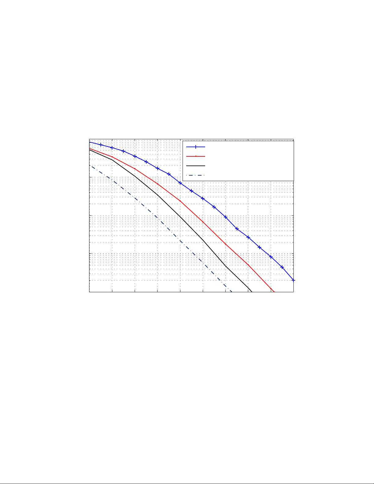
Cooperati v e T ransmission in a W ireless Relay Netw ork based on F lo w Management Debdeep Chatterjee, T an F . W ong, and T at M. Lok Abstract In th is p aper, a c oopera ti ve transmission de sign fo r a general m ulti-nod e half-du plex wireless relay network is presented. It is assumed that the nodes operate in half-dup lex mode and that channel informa tion is a vailable at the nodes. The pr oposed design in volv es solving a con vex flow optimization problem on a graph that m odels the relay n etwork. A much simpler generalized-lin k selection pro tocol based o n the above design is also presented . Both the pro posed flow-optimized proto col an d the generalized -link selection protocol are shown to achiev e the optimal diversity-multiplexing tradeoff (DMT) for the relay network. Moreover, simu lation results a re pr esented to q uantify the gap between the performance s of the pro posed p rotoco ls an d that o f a max-flow-min-cu t type bo und, in terms o f outage probability . I . I N T RO D U C T I O N A wireless relay network is one in which a set of relay nodes ass ist a source node transm it information to a destin ation n ode. Practically the wireless nodes can only support h alf-duplex communication [1], i.e., no nodes can recei ve and transmi t inform ation simu ltaneously on the same frequency band. Different cooperative transmission schem es for systems with half-duplex nodes have been proposed in the literature. Fundamentally , these schemes consist of two basic steps. First, the source transmits to the destin ation, and the relay l istens and “captures” [2] th e This research is supported in part by the National Science Foundation under Grant CNS-0626863 and by the Ai r Force Office of Sci entific Research under Grant F A9550-07-1045 6. A part of this work was presented at the IEE E Wireless Commun ications and Networking C onference (W CNC), Las V egas, March 2008. D. Chatterjee and T . F . W ong are with the Department of E lectrical and C omputer Engineering, Univ ersity of Florida, Gainesville, FL 32611-6130, U. S.A. e-mail: { debdeep,twong } @ufl .edu T . M. L ok is with Department of Information Engineering, The Chinese University of Hong Ko ng, Shatin, Hong Kong e-mail: tmlok@ie.cu hk.edu.hk 2 transmissio n from the source at the same time. Next, the relays send processed source information to the d estination whi le the so urce m ay still t ransmit to t he destination directly . V ariants of these techniques have been proposed and hav e been sh own to yield good p erformance under different circumstances [1], [3], [4]. Assuming channel state informati on (CSI) at t he nodes, an opportunist ic decode-and-forward (DF) proto col for half-duplex relay channels is propos ed in [5]. In [6], t he authors p resent routing algorithms t o opt imize the rate from a source to a desti nation, based on the DF techni que that uses regular bl ock Markov encoding and windowed decoding [7], [8], for the Gaus sian full- duplex multipl e-relay channel. The achiev able rate of [7] for the Gaussi an physically degraded full-duplex multi-relay channel has been establi shed as the capacity o f this channel in [9]. In [10], it is shown that the cut-set boun d on t he capacity of the Gaussian s ingle s ource-multiple relay-single destination mesh network can be achie ved usin g t he com press-and-forward (CF) method, as the relay powers go to infinity . Some simpler cooperative di versity methods based on network path selection hav e been recently report ed [11 ], [12 ]. Th ese s election methods include: (i) th e m ax-min s election met hod [11], wherein the relay node wi th the maximum of t he m inimum of the source-relay and relay- destination channel gains is selected; (ii) t he harmonic mean selectio n method [11], wherein the relay n ode with the highest harmonic mean of the source-relay and relay-destinati on channel gains is selected; and (iii) the selection schem e of [12], in which the relay that can correctly decode t he inform ation from the source and has the best relay-destination channel is selected. These methods achiev e a DMT of d ( r ) = ( N − 1)(1 − 2 r ) for an N node relay network and multiplexing gain 0 < r < 0 . 5 . This is close to what the distributed space-time cod ing protocol [13] achie ves, wh en N is large. Unfortunately , these network selection protocols perform poorly in high-rate scenarios ( r > 0 . 5 ). W e h a ve proposed a cooperative diversity design b ased on a flo w opt imization approach for a three-node network in [14]. In this design, the source node broadcasts t wo di stinct flo ws to the desti nation and the relay no de respectively during the relay’ s listen period. Then the relay forwards this information using the DF approach while the s ource m ay also send another flo w 3 of informati on to the destin ation during t he relay’ s transmit period. Thi s scheme is shown to achie ve the opti mal diversity order for the three-node relay channel and yield performance very close to optimal full-duplex relaying in both low- and hi gh-rate si tuations. Here, we apply this cooperati ve tra nsmiss ion design to a general relay network, wh erein wireless links are present between each pair of nodes i n the network. As in [14], assuming CSI is av ailable at all nodes we use broadcasting (BC), mu ltiple access (MA) and t ime sharing (TS) techniques to form ulate a flo w t heoretic con vex optimi zation prob lem b ased on the channel conditions. Instead of considering a total power constraint for a ll the transmitting nodes as in [14], we s ubject each node to a maximum transm it power const raint. Th is yi elds a m ore reasonable system model for a general wireless relay network, especially when the num ber of nodes in the relay network is large. The result ing relaying proto col will be referred to as the flow-optimized (FO) protocol. T o obtain a m ore pra ctical cooperati ve d esign we dev elop a generalized-link selection (GLS) proto col, in which we select t he best relay nod e out of the ava ilable ones to form an equiv alent three-node relay network to transmit the i nformation from th e source to the destination. The b enefit of t his, over other network path selection strategies, becomes evident when the rate requirement is high. It is shown that the simpl e GLS protocol is optim al in terms of the DMT [15] and yields acceptable performance eve n when th e rate requirement is high. Recently , in [16 ], the authors hav e shown th at compress-and-forward (CF) relaying achiev es the o ptimal DMT for the three-node, half-dupl ex network, and that DF relaying can achiev e the op timal DMT of the four-node full-duplex network. In this work, we show that the optimal DMT can be achieve d for a general N -node ( N ≥ 3 ) half-duplex network using the FO or GLS protocols. Here, it should be clarified that we con sider that the wireless links between each node-pair experience independent Rayleigh fading, and this corresponds to the definition of non-cluster ed networks in [16]. The performances of the FO and GLS protocols are ev aluated numerically in terms of their outage probabili ties for four- and fi ve-node relay networks for uniform and non-uni form a verage powe r gains. The num erical results motivate the us e of the GLS protocol for s ituations where com putation complexity is an issue and show a remarkable improvement over the m ax-min selection metho d of [11]. Th e p roposed designs, based on BC 4 and MA alone, are sub-optim al in general. For a fair app raisal of the proposed protocols, we compare th e propo sed protocols to an upper bou nd on the maximum rate, derived usi ng the max-flow-min-cut t heorem [17, Thm. 14.10.1]. I I . A G E N E RA L D E S I G N U S I N G A F L O W - T H E O R E T I C A P P R O AC H W e consider an N -node wireless relay network with a link joining each pair of nodes. Each such wireless link is d escribed by a bandpass Gauss ian channel with band width W and one-si ded noise sp ectral density N 0 . W e denote th e power gain of the link from node i to n ode j as Z ij . The link po wer gains are assumed to be in dependent and identi cally distributed (i.i.d.) exponential random va riables with unit mean. This corresponds to the case of independent Rayleigh fading channels wit h unit average power gains. M oreover , we assum e that each node has a maximu m power limit of P and can only support half-duplex transmissi on. Note that this model can be easily generalized to the case where channels m ay have n on-uniform avera ge power gains (for which numerical examples are presented in Section IV), and where differ ent nodes may have diffe rent maximu m power cons traints. More specifically , the latter case can be con verted i nto the unifo rm maximum power cons traints case by absorbing the no n-uniformity in th e t ransmit powers into the av erage power gains of the correspond ing links . In the sequel, we characterize the system in terms o f the transm it signal-to -noise ratio (SNR), S = P N 0 W , at the input o f t he links. Time is divided int o unit intervals, and BC and MA are applied with a TS st rategy that is optimized to m aximize the s pectral ef ficiency (which we call “rate” hereafter for con venience). T o av oid int erference between concurrent t ransmissions , a time interval is divided into slots : • Du ring the first s lot, the source may BC to all the other nodes in the network. • Du ring the subsequ ent slo ts, a relay may BC to all other nodes (except the source node), or it may recei ve flows from all other no des (except from the destinati on) through MA. • Du ring the very last slot, the source and the relays may send informati on flows to the destination using MA. Note t hat t he forwarding of information by the relays is based on the DF approach. For practi- cality consideration, it is assumed t hat the phases of the simultaneously transmitted signals from 5 diffe rent nod es are no t synchron ized. In general, for the above transmissio n protocol, there would be a maximum of 2( N − 2) + 2 = 2 N − 2 t ime slots of lengths t 1 , t 2 , · · · , t 2 N − 2 respectiv ely . Next, we d escribe the optimization problem u sing a graph-th eoretic formulation. Define a graph G = ( V , E ) , where V is th e set of nodes, E is the set of all link s joi ning the nodes in the graph, and associate the vector r to represent t he flow rates associated with each link in E . Thus, the number o f elements in r equals the cardinality o f E . For con venience, we write G = ( V , E , r ) . Now denote t he source b y S , the dest ination by D , and the relay nodes by R 1 , . . . , R N − 2 . The slot ting of a unit time interval, as described above, yields simpl er graphs for each time sl ot, that we call basic graphs . A b asic graph is either one i n whi ch a particular node may BC to s e veral nodes, or in which se veral nodes transmit via MA to a particular node. Thus for a basic graph, we need to in clude only the li nks between the nodes t hat may participate durin g the concerned tim e slot. For example, assum e that t he relay R 1 broadcasts to all nodes o ther t han the source, during the i -th t ime sl ot. The basic graph is g iv en by G i = ( V , E i , r i ) where V = {S , R 1 , · · · , R N − 2 , D } , E i = {R 1 R 2 , · · · , R 1 R N − 2 , R 1 D } , r i =  x i R 1 R 2 t i · · · x i R 1 R N − 2 t i x i R 1 D t i  T , where x i AB is the flow from node A to node B durin g the i -th time slot. In general, the prop osed design i n v olves TS between the basic graphs to yield the following equiv alent graph G corresponding to a unit interval (see [18] for a si milar idea): G = V , [ i E i , X i t i r i ! = t 1 G 1 + t 2 G 2 + . . . + t 2 N − 2 G 2 N − 2 . (1) where the number of elements i n each vector r i is extended to | S i E i | by inserting zeros appropriately . The second equality i n (1) i mplies that G can be vi e wed as a lin ear combin ation of the basic graphs G i s, with th e equivalent set of edges given by th e union of the sets E i , and the equiv alent flow rate vector given by the li near com bination of the ind ividual flow rate vectors r i . T o maximi ze the data rate from the s ource to the destinati on t hrough t he relay network, we need to consider each cut that partition s V into s ets V s and V d with S ∈ V s and D ∈ V d . Clearly , there can be 2 N − 2 such possi ble cuts for the N -node relay network. Let these cuts and 6 the correspondi ng cut sets be d enoted by C k , V s k , and V d k , respectively , for k = 1 , 2 , · · · , 2 N − 2 . Further , for the graph G , for any two nodes A ∈ V s k and B ∈ V d k , there exists a cut edge AB that cross es t he cut . Deno te t he to tal flo w th rough cut edge AB in a unit tim e interval by x AB = P 2 N − 2 i =1 x i AB . Now recall from network flow th eory [19] that the maxi mum flow rate from the source to the destination is specified by t he min imal cut of the equiv alent graph (1). Consequently , we arrive at th e following con vex flow optimizati on p roblem that can be so lved using standard optimizatio n techniques: max min    X A ∈ V s 1 ,B ∈ V d 1 x AB , X A ∈ V s 2 ,B ∈ V d 2 x AB , · · · , X A ∈ V s 2 N − 2 ,B ∈ V d 2 N − 2 x AB    (2) over all flow all ocations x i AB and all tim e slo t lengths t i , subject to • t he non-ne gativity constraint s : x i AB , t i ≥ 0 for all cut edges AB and i = 1 , 2 , · · · , 2 N − 2 , • t he to tal-time constraint : t 1 + . . . + t 2 N − 2 = 1 , • t he power (capacit y) constraints : – for a BC slot the flow rates s hould lie i n th e capacity re gion of th e BC channel wit h the transmitt ing node having a power constraint of P , – for an MA slot the flo w rates shou ld lie in the capacity region of the MA channel with a maximum power constraint P for each transmitting no de, • t he flow constraints : cons idering st eady stat e operation , the total information flo w out of a relay should equ al the flow into the relay in each unit time interval. Note that the dependence of the o bjectiv e function on the channel gains and t he tim e slot lengt hs is implicitly e xpressed t hrough the capacity constrain ts. Denot e the cut separating S from all t he other nodes and th e cut separating D from all nodes as C S and C D , respectively . Then we observe that the cost function in (2 ) above can be further s implified to max min { x ( C S ) , x ( C D ) } , where x ( C S ) = x S D + N − 2 X j =1 x S R j and x ( C D ) = x S D + N − 2 X i =1 x R i D (3) are the t otal flows across the above-mentioned cut s C S and C D , respecti vely . T o see this , con- sider the cut C with V s = { S , R 1 , · · · , R l } , and V d = {R l +1 , · · · , R N − 2 , D } for some l ∈ 7 { 1 , 2 , · · · , N − 2 } . The t otal flo w across this cut is given by x ( C ) = x S D + N − 2 X j = l +1 x S R j + l X i =1   x R i D + N − 2 X j = l +1 x R i R j   . (4) Now , consider no de i for i ∈ { 1 , 2 , · · · , l } . According to the flow constraint for node i , x R i D + N − 2 X j = l +1 x R i R j + l X k =1 ,k 6 = i x R i R k = x S R i + N − 2 X j = l +1 x R j R i + l X k =1 ,k 6 = i x R k R i . (5) Summing (5) over all i ∈ { 1 , 2 , · · · , l } we get l X i =1   x R i D + N − 2 X j = l +1 x R i R j   = l X i =1   x S R i + N − 2 X j = l +1 x R j R i   . (6) Since P l i =1 P N − 2 j = l +1 x R j R i ≥ 0 , combining (3), (4) and (6) gives x ( C ) ≥ x ( C S ) . Simil arly , we hav e x ( C ) ≥ x ( C D ) . Thus the cost function in (2) reduces to the above-mentioned form. I I I . G E N E R A L I Z E D - L I N K S E L E C T I O N A N D I T S O P T I M A L I T Y In this secti on, we present the GLS protocol and establish the opti mality of the FO and GLS protocols in terms of the DMT . This is accompli shed in three s teps. First, we apply the FO protocol to the th ree-node relay network. Next, we prop ose the GLS protocol based on a selection strategy t hat is sub-optim al to the FO protocol of Section II. Finally , the optimality of the GLS protocol, and thereby , t hat of the FO protocol, is established. A. The Thr ee-node Rela y Network The three-node relay network consists of a source ( S ), a relay ( R ), and a dest ination ( D ). W e specialize the general d esign described in the previous secti on to this th ree-node relay network. A uni t tim e i nterval is divided into two time slots of lengths t 1 and t 2 with t 1 + t 2 = 1 . During the first tim e slot, S sends (via BC) two flows of rates x 1 S D /t 1 = x 1 /t 1 and x 1 S R /t 1 = x 2 /t 1 to D and R , respectiv ely , resul ting in the basic graph G 1 . During the second time slot , R and S send (vi a MA) two flo ws of rates x 2 RD /t 2 = x 4 /t 2 and x 2 S D /t 2 = x 3 /t 2 to D , respectively , resulting in the basic graph G 2 . Combining the two b asic graphs yields the equiv alent graph 8 as G = t 1 G 1 + t 2 G 2 . Note that the information flo w of rate x 4 /t 2 sent by R du ring the MA time slot is from the flo w of rate x 2 /t 1 it receiv ed during the BC tim e slo t. Thus, we have the flo w constraint x 4 = x 2 . The rate for this network is s pecified by the m in-cut wh ich is clearly min { ( x 1 + x 2 + x 3 ) , ( x 1 + x 4 + x 3 ) } . H ence, the flow optim ization problem is given by: max min { ( x 1 + x 2 + x 3 ) , ( x 1 + x 4 + x 3 ) } (7) over flow allocati ons x 1 , x 2 , x 3 , x 4 , and time slot lengths t 1 , t 2 , subject to • n on-ne g ativity const raints: x 1 , x 2 , x 3 , x 4 ≥ 0 , t 1 , t 2 ≥ 0 , • t otal-time con straint: t 1 + t 2 = 1 , • p ower constraints: S B C ≤ S, x 1 ≤ t 1 C ( Z S D S ) , x 2 ≤ t 1 C ( Z S R S ) for the BC slot, x 3 ≤ t 2 C ( Z S D S ) , x 4 ≤ t 2 C ( Z RD S ) , x 3 + x 4 ≤ t 2 C ( Z S D S + Z RD S ) for th e MA slot, • fl ow constraint: x 2 = x 4 , where C ( x ) = log (1 + x ) , and S B C , the minimu m SNR required for th e source t o broadcast at rates x 1 /t 1 and x 2 /t 1 to the destination and the relay , respectiv ely , in the first time slot with 0 < t 1 ≤ 1 , is given by (see [14, Lemma 3.1] for proof) S B C =      1 Z S D ( e x 1 /t 1 − 1) + 1 Z S R e x 1 /t 1 ( e x 2 /t 1 − 1) for Z S R > Z S D , 1 Z S R ( e x 2 /t 1 − 1) + 1 Z S D e x 2 /t 1 ( e x 1 /t 1 − 1) for Z S R ≤ Z S D . For t 1 = 0 , S B C = 0 . Not e that for the BC slot , the last two constraints are redundant when t 1 > 0 , and compl ements the first constraint when t 1 = 0 . The s olution of this flo w o ptimization problem is giv en in Appendix A. As mentioned in Section I, the above op timization p roblem formu lation is differe nt from t hat in [14] wherein the sum of the source and relay power s, required to achieve a certain data rate, is minimi zed. More specifically , when considering individual power constraints for each node, we cannot use part 2 of [14, Lemma 3.1] to describe t he power constraints for the MA slot. T his is because doing so would restrict the flows x 2 and x 3 such that the sum of powers expended at S and R is minimized. O n the ot her hand, in the present problem, the po wer constraint s only dictate that the flow-ra tes should li e in the MA capacity region specified by the maximum power av ailable 9 at each transm itting node, for the particular fading state. W it h this mod ification in the constraint for the M A slot, the so lution approach to the abov e problem needs to b e markedly differ ent from that in [14] as shown in Appendi x A. The maximum information rate from the source S to the destination D for different cases is summ arized below: a) Z S D ≥ Z S R : The maximum rate is X ( S ) = C ( Z S D S ) with direct transmis sion from S to D . b) Z S D < Z S R : The maximum rate is X ( S ) = max 0 ≤ t 2 ≤ t 2 max t 1 log     1+ Z S D S 1+ Z S D Z S R   1+ Z RD S 1+ Z S D S  t 2 /t 1 − 1      + t 2 C ( Z S D S + Z RD S ) wit h t 2 max = C ( Z S R S ) / [ C ( Z S R S ) + C ( Z RD S + Z S D S ) − C ( Z S D S )] and t 1 = 1 − t 2 . Thus for a given power limit (i.e. a given S ) at the n odes, relaying is advantageous only when Z S D < Z S R . Further , the optimal solution always allocates a non-zero flo w to t he direct lin k. Also, the relay-destinati on link gain Z RD does not influence the strategy of transmis sion (i.e. whether to us e only the direct l ink or both t he relay and di rect links), but o nly the amoun t of information through the relay link. B. Generalized-link S election For the general N -node relay n etwork, the flow optimizati on solution can be computational ly demanding ev en for mod erate values of N . The G LS protocol described below provides a s imple sub-optimal design t o address this comp lexity issue. In essence, the G LS protocol i dentifies the best relay path out of the pos sible N − 2 relay paths and con siders only th e chosen relay alo ng with the source and destination to form a three-node relay network, w hich we call a gener alized- link from th e source t o the d estination, for information transm ission. In o ther words, the aim is to choose the best relay such that the equiv alent three-node relay network obtained (containing the sou rce, desti nation and th e chosen relay) gi ves th e m aximum rate over all possible equiv alent three-node n etworks contai ning t he s ource and destination. M ore p recisely , we need to consider the following p ossibili ties: 1) Z S D ≥ Z S R i for a ll i ∈ I = { 1 , 2 , · · · , N − 2 } : From the r esults of the optim ization problem (7), it i s clear that the maximum rate would be C ( Z S D S ) with direct transm ission o f all data from the source to the destinati on withou t u sing any relay . 10 2) There exists a k ∈ I such th at Z S R k > Z S D : Let th e s et of all such node indices be K and for all i ∈ I \ K , Z S D ≥ Z S R i . For this case, choose the node R ′ k as the relay such that k ′ = arg max k ∈ K X k ( S ) , where X k ( S ) is the m aximum rate for the three-node relay network with the so urce S , th e relay R k and destination D . In terms of t he worst-case computati onal comp lexities for t he FO and GLS protocols, it can be seen that, for an N -node relay network wi th N > 3 , the FO proto col in volves a max-min optimizatio n over 2( N 2 − 2 N + 2) variables (all possible flows and time slot lengths), su bject to N − 1 n on-linear and 2( N 2 − N + 1 ) linear constraints, whereas the GLS protocol in v olves a maximum of N − 2 maximization s of a non-linear conca ve function over two variables, subject to two linear constraints , followed by finding the maxim um of N − 2 real numbers wit h a worst-case complexity o f O ( N − 2 ) . Moreove r , for N > 3 , for the FO protocol, the BC slots potentially in v olve ( N − 1) - and ( N − 2) -lev el superposition coding (SPC) or dirty paper coding (DPC) implementati ons for S and the relays resp ectiv ely , whi le t he MA slots at the relays and D may inv o lve a maximum of ( N − 3) and ( N − 2) int erference cancelation (IC) operations respectiv ely . On th e o ther hand, the GLS protocol in volves a maxi mum of 2 -le vel SPC/DPC and one IC operation for the BC and MA slots respectiv ely , for any N > 3 . C. Diversity-multiplexing tradeoff As in [15 ], the mu ltiplexing gain r = lim S → ∞ R ( S ) log S where S is the SNR and R ( S ) is the rate at an SNR level of S . Following [15], we parameterize t he sy stem, in terms of the SNR S and the multip lexing gain, 0 < r < 1 , with the rate increasing with the SNR as R = r log( S ) . With the parameterization ( r , S ) , t he diver sity order achieved by the transmiss ion scheme is given by d ( r ) = lim S → ∞ − log P e ( r , S ) log S (8) where P e ( r , S ) is the aver age probabi lity of error when the SNR i s S and m ultiplexing gain r . The following th eorem, whose proof i s outlined in Appendix B , establishes the op timality of the the GLS protocol (and hence the FO protocol ) in terms of the DM T : 11 Theor em 3 .1: The GLS and FO protocol s achieve t he opti mal DMT d ( r ) = ( N − 1)(1 − r ) for all 0 < r < 1 , for the N -node half-duplex wireless relay net work. I V . N U M E R I C A L E X A M P L E S Using the outage probability as the per formance metric, we compare the FO and GLS protocols against the max-min selection m ethod of [11], as it provides the best performance amongst pre viously p roposed path selection methods, and an outage probability lower bound deri ved using the max-flo w-min-cut theorem of [17, Thm. 14.10.1]. For th e four-node relay network, there can be 6 possi ble time slots i n the FO protocol as shown i n Fig. 1. T o derive an upper bound on t he achie v able rate (and thereby a lower bound on the outage p robability), we us e max-flow-min-cut ty pe bound s for half-dupl ex com munication. There are four poss ible t ime sl ots as shown i n Fig. 2, with the first BC sl ot and t he last M A slot at th e destinati on same as in the FO protocol, but now , the source and a relay may transmit simultaneous ly to the other relay and the destinati on during each o f the i ntermediate slots over interference channels. W e use the max-flow-min-cut theorem to u pper bound the maximum information flo w in these two t ime slots. For the fiv e-node relay network, t here can be 8 possibl e tim e sl ots in the FO protocol - four BC slots for t he s ource and the t hree relays to t ransmit i nformation, and four MA slots for the three relays and th e destination to receiv e information respective ly . Sim ilar to the four-node relay n etwork case, for the max-flow-min-cut bound, there are 8 possible time slots with the first BC slot and the last MA slot at the d estination being the same as for t he FO p rotocol, and multi-source-mul ti-destination transmission s during the six int ermediate slots . W i th the above division of time slots, the formalizatio n o f the problem is done as in the pre vious secti ons, and we use the opt imization routine of [20] to ob tain the maximum achi e vable rates and upper bounds for di ff erent values of required ra tes. In Figs . 3 and 4, we plot the outage probabili ties of the various schemes with the required rate R at 1 bit/ s/Hz and 6 bits /s/Hz respectiv ely , for the four-node relay network. Figs. 5 and 6 present the same for the five-node relay network. When com pared to t he FO protocol, the GLS protocol suffers a los s of around 12 1 . 0 dB, and around 1 . 5 dB (when R is either 1 bit/s/Hz or 6 bits /s/Hz), at an outage probabi lity of 10 − 4 , for the four- and fi ve- node relay networks respective ly . On the ot her hand, the performance degradation for the max-min selection method of [11], as compared to the F O protocol or ev en the GLS p rotocol, is more than 12 dB at an outage probability of 7 . 0 × 10 − 2 , when R = 6 bits /s/Hz for the four-node relay network, and an exactly sim ilar s ituation can be observed for the five- node relay network. M oreover , for the four-node relay network, the FO protocol is within 2 . 14 dB (when R = 1 bit/s/Hz) to wit hin 7 . 05 dB (when R = 6 bits/ s/Hz) of the lower bound on t he outage probability when t he ou tage prob ability is 10 − 4 . For the five- node relay network, the corresponding differe nces are approximately 3 dB and 9 . 6 dB respectively . The performances of the differe nt protocols for t he four -node relay n etwork wit h non -uniform a verage power gains are presented in Figs. 7 and 8, and Figs. 9 and 10 for cases A and B respectiv ely , wit h the av erage power gains as stated in the figures. In case A, t he source-relay links are, on avera ge, better t han the direct link, and one relay nod e i s, on avera ge, a bett er candidate to forward the information to D . On t he other hand, in case B, no one relay has very good s ource-relay and relay-destination lin ks, whereas the i nter-r elay li nk is , on a verage, very good. This promotes in creased inter-relay flo ws wh en usin g the FO protocol, and thereby highlight s the l imitatio ns of the GLS prot ocol. Th e dif ferences between the out age performances of th e FO and GLS protocols, at an outage probabi lity of 10 − 4 , are 1 . 2 dB or 1 . 0 d B, and 2 . 0 dB or 1 . 3 dB (when R = 1 bi ts/s/Hz or R = 6 bits/s/ Hz), for cases A and B respectiv ely . Thu s, the gap between the FO and GLS protocols decreases as t he required dat a rate increases. When the required rate is high, th e codi ng gain offe red by a protocol heavily relies on the efficient use o f the direct li nk, and s ince the usage of the direct link is sim ilar for bot h the FO and the GLS protocols, the performance gap narro ws as the required data rate increases. On t he other hand, at the s ame out age probabilit y , t he di ff erence between the outage performance of the FO protocol and the lower bound increases from 1 . 5 dB to 7 dB, and from 1 . 9 d B to 6 . 0 dB as the required rate increases from 1 b it/s/Hz to 6 b its/s/Hz, for cases A and B respectively . Overa ll, these results demonstrate trends s imilar to t he uniform avera ge power gain case, and confirm the generality of the proposed protocols. 13 V . C O N C L U S I O N S W e proposed a cooperative transmission design for a general m ulti-node half-duplex wi reless relay network. It is based on optimizing information fl ows, using the basic c omponents of BC and MA, to maximize the transm ission rate from the s ource to the destinat ion, su bject to m aximum power c onstraints at ind ividual nodes. W e also p roposed the simpler GLS protocol, that combines relay selection, and fl ow optimization for a three-node relay network. These protocols were sho wn to achie ve the opt imal DM T for a general relay network. Simulation results for the fou r - and fi ve-node relay networks for uniform and non-uniform av erage po wer g ains demonstrate that the performance of the much simpler G LS protocol is close to that of the FO protocol. Thi s suggests that the GLS protocol can be used in system s wi th low-complexity requirements. W e also note that the proposed FO and GLS protocols can be us ed in wireless networks with topologies more complicated that the wireless relay network considered here. For e xample, application of similar ideas t o a parallel relay network in which th ere is no di rect connectio n between the source and the destination is considered in [21]. A P P E N D I X A. Solut ion to optim ization pr oblem (7) W e consider two cases with re gard to the lin k gains: (a) Z S D ≥ Z S R , and (b) Z S D < Z S R . For both cases, w e solve the opt imization problem in two stages: first, we fix t 1 , t 2 ≥ 0 such that t 1 + t 2 = 1 and find the o ptimal flows x 1 , x 2 , x 3 in terms of t 1 , t 2 , and then, find the optimal va lues for t 1 , t 2 to maximize the objective function . a) Z S D ≥ Z S R : T o obtain an analytical so lution to the optimizati on problem and better insight i nto t he nature of the solution t o the flow op timization problem, we modi fy the repre- sentation of the BC slot power constraint from that in (7) to the one that is more con ventionall y used to describe the capacity region of the Gaussian BC channel, as presented in (9). Using the flo w constraint in (7), we first solve (9) for fixed t 1 , t 2 . max( x 1 + x 2 + x 3 ) over x 1 , x 2 , x 3 , α, subject to (9) 14 x 1 , x 2 , x 3 ≥ 0 , 0 ≤ α ≤ 1 , x 1 ≤ t 1 C ( Z S D αS ) , x 2 ≤ t 1 C  Z S R ¯ αS 1 + Z S R αS  , x 2 ≤ t 2 C ( Z RD S ) , x 3 ≤ min { t 2 C ( Z S D S ) , t 2 C ( Z S D S + Z RD S ) − x 2 } . Here, α ∈ [0 , 1] is the fraction of total power s pent at t he source to transmi t x 1 directly t o the destination during the BC slot, and ¯ α = 1 − α . Although, this modification of the BC slot power constraint apparently makes the opt imization p roblem non-con ve x owing t o the no n-con ve xity in α , as we shall see in the sequel, this issue can b e handled easily b y utilizing the monotonicity of the logarithm fun ction. Denote the opt imal soluti on by ( x ∗ 1 , x ∗ 2 , x ∗ 3 , α ∗ ) and the corresponding m aximum rate by X ( t 1 , t 2 ) . It is clear that x ∗ 1 = t 1 C ( Z S D α ∗ S ) . Suppose that x ∗ 2 < t 1 C  Z S R ¯ α ∗ S 1+ Z S R α ∗ S  . Since t 1 C  Z S R ¯ αS 1+ Z S R αS  is a decreasing functi on of α , we can increase α from α ∗ to α 0 such that x 0 1 = t 1 C ( Z S D α 0 S ) > x ∗ 1 and x ∗ 2 = t 1 C  Z S R ¯ α 0 S 1+ Z S R α 0 S  . T hus th e objecti ve functi on becomes ( x 0 1 + x ∗ 2 + x ∗ 3 ) > ( x ∗ 1 + x ∗ 2 + x ∗ 3 ) at α 0 . This contradicts the optimality of ( x ∗ 1 , x ∗ 2 , x ∗ 3 , α ∗ ) . As a consequence, we ha ve x ∗ 2 = t 1 C  Z S R ¯ α ∗ S 1+ Z S R α ∗ S  ≤ t 2 C ( Z RD S ) . This implies that α ∗ ≥ max    1 Z S R S " 1 + Z S R S (1 + Z RD S ) t 2 /t 1 − 1 # | {z } α a 0 , 0    , and α 0 a ≤ 1 . In essence, this means that th e optimal x 1 and x 2 should lie on the boundary of the degraded BC capacity region. W ith this, it is obvious then that x 3 = min n t 2 C ( Z S D S ) , t 2 C ( Z S D S + Z RD S ) − t 1 C  Z S R ¯ αS 1+ Z S R αS o . Therefore the optimi zation problem of (9) can be re-written as: max ( x 1 + x 2 + x 3 ) (10) subject to max { 0 , α 0 a } ≤ α ≤ 1 , x 1 = t 1 C ( Z S D αS ) , x 2 = t 1 C  Z S R ¯ αS 1 + Z S R αS  , x 3 = min  t 2 C ( Z S D S ) , t 2 C ( Z S D S + Z RD S ) − t 1 C  Z S R ¯ αS 1 + Z S R αS  . W e observe that x 3 = t 2 C ( Z S D S ) above if and o nly if α ≥ 1 Z S R S    1 + Z S R S  1 + Z RD S 1+ Z S D S  t 2 /t 1 − 1    , α 1 a . (11) 15 Comparing this to the expression for α 0 a giv es α 0 a ≤ α 1 a ≤ 1 . Next we consider two possibl e sub-cases: i. t 2 C  Z RD S 1+ Z S D S  ≤ t 1 C ( Z S R S ) : In this case, we h av e ¯ α 1 a ≥ 0 and t 2 ≤ C ( Z S R S ) C  Z RD S 1+ Z S D S  + C ( Z S R S ) , t 2 max . The maximum rate can be expressed as X ( t 1 , t 2 ) = max { X 1 ( t 1 , t 2 ) , X 2 ( t 1 , t 2 ) } where X 1 ( t 1 , t 2 ) = max max { 0 ,α 0 a }≤ α ≤ α 1 a t 1 C ( Z S D αS ) + t 2 C ( Z S D S + Z RD S ) = t 1 C ( Z S D α 1 a S ) + t 2 C ( Z S D S + Z RD S ) ≤ t 1 log (1 + Z S D α 1 a S )(1 + Z S R S ) 1 + Z S R α 1 a S ! + t 2 C ( Z S D S ) ≤ C ( Z S D S ) (12) X 2 ( t 1 , t 2 ) = max α 1 a ≤ α ≤ 1 t 1 C ( Z S D αS ) + t 1 C  Z S R ¯ αS 1 + Z S R αS  + t 2 C ( Z S D S ) = C ( Z S D S ) (13) where t he first inequality in (12) holds s ince (11) is n ot sati sfied, and the second inequ ality in (12) holds since α 1 a ≤ 1 and that the first term in the pre vious step is m onotonically increasing in α 1 a when Z S D ≥ Z S R . This way , the last observation helps a void the non- con vexity is sue m entioned before. Similar ar guments hold for X 2 ( t 1 , t 2 ) in (13). ii. t 2 C  Z RD S 1+ Z S D S  > t 1 C ( Z S R S ) : In this case, we hav e α 1 a < 0 and t 2 > t 2 max . Thus the maximu m rate is given by X ( t 1 , t 2 ) = max 0 ≤ α ≤ 1 t 1 C ( Z S D αS ) + t 1 C  Z S R ¯ αS 1 + Z S R αS  + t 2 C ( Z S D S ) = C ( Z S D S ) . (14) Hence, (12)–(14) imply that the solution to (9), for any t 1 , t 2 pair , occurs at α = 1 , and the s olu- tion to the original problem of (7), when Z S D ≥ Z S R , is given by max { 0 ≤ t 1 ,t 2 : t 1 + t 2 =1 } X ( t 1 , t 2 ) = C ( Z S D S ) with any t 1 , t 2 pair su ch that t 1 , t 2 ≥ 0 and t 1 + t 2 = 1 . b) Z S D < Z S R : In t his case, the source-relay link is bett er than the so urce-destination lin k. Again, we first fix time slo t lengt hs t 1 and t 2 and solve for the optimal values of x 1 , x 2 , x 3 , and α , and then maxim ize the objective function of (7) over all feasible time slot leng ths. Following 16 similar arguments as in Case a), the optim ization prob lem of (7) can be re-written as: max ( x 1 + x 2 + x 3 ) (15) subject to 0 ≤ ¯ α ≤ min { 1 , ¯ α 0 b } , x 1 = t 1 C  Z S D αS 1 + Z S D ¯ αS  , x 2 = t 1 C ( Z S R ¯ αS ) , x 3 = min { t 2 C ( Z S D S ) , t 2 C ( Z S D S + Z RD S ) − t 1 C ( Z S R ¯ αS ) } where ¯ α 0 b = 1 Z S R S h (1 + Z RD S ) t 2 /t 1 − 1 i is an upper bound on ¯ α such that t 1 C ( Z S R ¯ αS ) ≤ t 2 C ( Z RD S ) . As before, x 3 = t 2 C ( Z S D S ) if and only if ¯ α ≤ 1 Z S R S   1 + Z RD S 1+ Z S D S  t 2 /t 1 − 1  , ¯ α 1 b . Also, 0 ≤ ¯ α 1 b ≤ ¯ α 0 b . Again , we cons ider two pos sible sub -cases: i. t 2 C  Z RD S 1+ Z S D S  ≤ t 1 C ( Z S R S ) : In this case we have ¯ α 1 b ≤ 1 and t 2 ≤ C ( Z S R S ) C  Z RD S 1+ Z S D S  + C ( Z S R S ) , t 2 max . The maximum rate X ( t 1 , t 2 ) can be expressed as X ( t 1 , t 2 ) = max { X 1 ( t 1 , t 2 ) , X 2 ( t 1 , t 2 ) } wh ere X 1 ( t 1 , t 2 ) = max 0 ≤ ¯ α ≤ ¯ α 1 b t 1 C  Z S D αS 1 + Z S D ¯ αS  + t 1 C ( Z S R ¯ αS ) + t 2 C ( Z S D S ) , (16) X 2 ( t 1 , t 2 ) = max ¯ α 1 b ≤ ¯ α ≤ min { 1 , ¯ α 0 b } t 1 C  Z S D αS 1 + Z S D ¯ αS  + t 2 C ( Z S D S + Z RD S ) , (17) and both t he maxima i n (16) and (17) are attained at ¯ α = ¯ α 1 b . Subst ituting the expression for ¯ α 1 b in (16) and (17), we obtain X 1 ( t 1 , t 2 ) = X 2 ( t 1 , t 2 ) and X ( t 1 , t 2 ) = t 1 log     1 + Z S D S 1 + Z S D Z S R   1 + Z RD S 1+ Z S D S  t 2 /t 1 − 1      + t 2 C ( Z S D S + Z RD S ) . (18) ii. t 2 C  Z RD S 1+ Z S D S  > t 1 C ( Z S R S ) : In this case we hav e ¯ α 1 b > 1 and t 2 > t 2 max . Thu s t he maximum rate is given by X ( t 1 , t 2 ) = max 0 ≤ ¯ α ≤ 1 t 1 C  Z S D αS 1 + Z S D ¯ αS  + t 1 C ( Z S R ¯ αS ) + t 2 C ( Z S D S ) = t 1 C ( Z S R S ) + t 2 C ( Z S D S ) (19) where the maxim um occurs at ¯ α = 1 , as the function t o be maximi zed i s m onotonically increasing in ¯ α when Z S R > Z S D . 17 Finally , we opti mize the above solu tion to (15) over all possib le time slot length s to obtain the solution to the origi nal problem in (7) when Z S D < Z S R . Corresponding to Case i. above, when t 2 ≤ t 2 max , we no te that max { 0 ≤ t 1 ,t 2 : t 1 + t 2 =1 } X ( t 1 , t 2 ) ≥ X (1 − t 2 , t 2 ) | t 2 = t 2 max = C ( Z S R S ) C ( Z S D S + Z RD S ) C ( Z S R S ) + C ( Z RD S + Z S D S ) − C ( Z S D S ) . (20) On the other hand, corresponding to Case ii., when t 2 > t 2 max , from (19), we hav e max { 0 ≤ t 1 ,t 2 : t 1 + t 2 =1 } X ( t 1 , t 2 ) < (1 − t 2 max ) C ( Z S R S ) + t 2 max C ( Z S D S ) = C ( Z S R S ) C ( Z S D S + Z RD S ) C ( Z S R S ) + C ( Z RD S + Z S D S ) − C ( Z S D S ) (21) where the in equality in (21) is ob tained from (19) by using Z S R > Z S D and t 2 > t 2 max . Hence, from (20) and (21 ), we conclude that when Z S R > Z S D , the maximum achiev able rate is g iv en by X ( S ) = max 0 ≤ t 2 ≤ t 2 max t 1 log     1+ Z S D S 1+ Z S D Z S R   1+ Z RD S 1+ Z S D S  t 2 /t 1 − 1      + t 2 C ( Z S D S + Z RD S ) . B. Pr oof of Theor em 3.1 In this appendix, we sketch th e proof of the theorem. Part 3) of Theorem 4.2 of [14] can be generalized for the N -node relay network to prove that, as t he block length goes to infinity (during any particular time in terval), the av erage error probabil ity for the FO prot ocol is upper bounded by its c orresponding out age probabili ty . Here, the outage probability denotes th e probabili ty that th e d ata rate R cannot be supported by the system when the SNR is S , i.e., P out ( r , S ) = Pr[ X ( S ) < r log S ] w here X ( S ) d enotes the maximum rate possib le for the given channel gain realizations when the SNR is S . Thus, from the definition of diversity order (8), we have d ( r ) ≥ lim S → ∞ − log P out ( r , S ) log S . (22) Moreover , the abo ve result fr om [14] can be directly used to prove the same for the GLS protocol. Using this fact, we deriv e a lower bound to the DM T that can be achieved by the GLS prot ocol. 18 The sets I and K , used in the sequel, are the sets of i ndices as described in Section III-B. T he outage p robability for the GLS protocol is given b y P gr out ( r , S ) = Pr  max k ∈ I X k ( S ) < r log S  (23) where X k ( S ) is the maximum rate achieva ble by the three-node relay network formed by the source S , the relay R k and the destination D . W e have the following possibi lities: • Case A: | K | = 0 , i.e. the cardinality of the set K is zero. T his correspond s to the case when Z S D ≥ Z S R k for all k ∈ I . • Case B: | K | = i wi th i ∈ I . Note that for Case B there are  N − 2 i  possibili ties for the set K with cardinality i . Since th e link g ains are assum ed to be i.i.d., and the outage probability depends on t he distribution of the maximum o f X k ( S ) over all k ∈ I (or effecti vely , over all k ∈ K when | K | > 0 ), only the cardinality of K is significant. Let the  N − 2 i  possible constru ctions of t he set K be represented by a “generic” set K 0 with cardinality i . W i thout los s of generality , we describe K 0 as the set K corresponding to the case when the i ndices of th e relay no des are o rdered according to t heir source-relay link gain s, i.e. Z S R 1 ≥ Z S R 2 ≥ · · · ≥ Z S R N − 2 . Thus, Case B n ow im plies a so litary choice for set K , viz. K 0 = { 1 , 2 , · · · , i } . Therefore, from (23), we hav e P gr out ( r , S ) = Pr ( C ( Z S D S ) < r log S | | K 0 | = 0 ) Pr( | K 0 | = 0 ) + N − 2 X i =1 Pr  max k ∈ K 0 X k ( S ) < r log S     | K 0 | = i  Pr( | K 0 | = i ) . (24) W e o bserve that us ing th e right-m ost expression of (20) in stead of X k ( S ) , for each k ∈ K 0 , in (24) gives an upper bound on P gr out ( r , S ) . This is utilized i n obtaining a lower bound on the diversity order of the GL S p rotocol. Let { S n } ∞ n =1 be an increasing u nbounded sequence of SNRs with S 1 > 1 . D efine t he sequence of random variables { M k n } ∞ n =1 , { B k n } ∞ n =1 and { A k n } ∞ n =1 with M k n = C ( Z S R k S n ) − C ( Z S D S n ) C ( Z S D S n + Z R k D S n ) , B k n = C ( Z S R k S n ) log S n , and A k n = X k ( S n ) log S n = B k n 1+ M k n , resp ectiv ely . Note that for all k ∈ K 0 , M k n → 0 a.s. This implies t hat ( B k n − A k n ) → 0 a.s . Define A ′ n = max k ∈ K 0 A k n and B ′ n = max k ∈ K 0 B k n (= B 1 n ) . Then using the above, it can be see n 19 that ( B ′ n − A ′ n ) → 0 a.s. Further , lim n →∞ Pr ( B ′ n < r | | K 0 | = i ) exists, and t herefore t he above implies that lim n →∞ Pr ( A ′ n < r | | K 0 | = i ) = lim n →∞ Pr ( B ′ n < r | | K 0 | = i ) . Using this in (22) and (24), the div ersity order for the GL S protocol, d gr ( r ) , satisfies d gr ( r ) ≥ lim S → ∞ − log P gr out ( r , S ) log S ≥ lim n →∞ − 1 log S n log  Pr  Z S D < S r n − 1 S n     | K 0 | = 0  Pr( | K 0 | = 0 ) + N − 2 X i =1 Pr  Z S R 1 < S r n − 1 S n     | K 0 | = i  Pr( | K 0 | = i ) # (25) = lim n →∞ − 1 log S n log  Pr  max { Z S D , Z S R 1 , · · · , Z S R N − 2 } < S r n − 1 S n     | K 0 | = 0  Pr( | K 0 | = 0 ) + N − 2 X i =1 Pr  max { Z S D , Z S R 1 , · · · , Z S R N − 2 } < S r n − 1 S n     | K 0 | = i  Pr( | K 0 | = i ) # (26) = lim S → ∞ − log  Pr  max { Z S D , Z S R 1 , · · · , Z S R N − 2 } < S r − 1 S  log S = lim S → ∞ − log  [1 − exp ( − ( S r − 1) /S )] N − 1  log S = ( N − 1)(1 − r ) (27) where (26) i s obtained from (25) by n oting that max { Z S D , Z S R 1 , · · · , Z S R N − 2 } = Z S D when | K 0 | = 0 , and max { Z S D , Z S R 1 , · · · , Z S R N − 2 } = max k ∈ K 0 Z S R k = Z S R 1 when | K 0 | > 0 , the first equality in (27) is du e to t he link gai ns being i .i.d., and the s econd equality i n (27) is obtained by using L ’Hospi tal’ s rule. Next given an N -node relay network, consider th e multiple access cut that separates the destination from all the other no des. Clearly , the total flo w across this cut gives an upper bound on the maxim um rate achiev able in the N -node relay n etwork. Consequentl y , a lower bo und on the outage probability P l out ( r , S ) can be obtained using t he maximum sum-rate across this cut: P l out ( r , S ) ≥ Pr h C (( Z S D + Z R 1 D + · · · + Z R N − 2 D ) S ) < r log S i = Pr h ( Z S D + Z R 1 D + · · · + Z R N − 2 D ) < x i = γ ( N − 1 , ( S r − 1) /S ) Γ( N − 1) , (28) where γ ( a, x ) = R x 0 t a − 1 e − t dt is the lower incom plete gamma function and Γ( a ) = R ∞ 0 t a − 1 e − t dt is th e complete gamma function. Th e resul t in part 1) of Theorem 4.2 of [14] can be extended to 20 show that the diver sity o rder of any transmiss ion scheme over the wi reless relay network must satisfy d ( r ) ≤ lim S → ∞ − log  P l out ( r , S )  log S ≤ lim S → ∞ − log  γ ( N − 1 , ( S r − 1) /S ) ( N − 2)!  log S = − lim S → ∞ e − x x N − 2 [ S − 1 − (1 − r ) S r − 1 ] R x 0 t N − 2 e − t dt = ( N − 1)(1 − r ) . (29) Finally , from (27) and (29), we see that the GLS prot ocol, and hence the FO proto col, achie ve the optimal DMT of ( N − 1)(1 − r ) for al l 0 < r < 1 . R E F E R E N C E S [1] J. N. Laneman, D. N. C. Tse, and G. W . W ornell, “Cooperativ e Di versity in Wireless Networks: Efficient P rotocols and Outage Behavior , ” IE EE T ransac tions on I nformation Theory , vol. 50, no. 12, pp. 3062–3080 , Dec. 2004. [2] A. Host-Madse n, and J. Zhang, “Capacity bounds and power allocation for wi reless relay channels, ” IEE E T ransa ctions on Information Theory , vol. 51, no. 6, pp. 2020–2040 , June 2005. [3] K. Azarian, H. El Gamal, and P . Schniter , “On the achie v able di versity-multiplex ing tradeoff in half-duplex cooperativ e channels, ” IEEE T ransaction s on Information Theory , vol. 51, no. 12, pp. 4152–4 172, Dec. 2005. [4] A. S. A vestimehr , and D. N. C . Tse, “Outage capacity of the fading relay channel in low SNR r egime, ” IEEE T ra nsactions on Information Theory , submitted for publication, Feb . 2006. [5] D. Gunduz, and E. Erkip, “Opportunistic cooperation by dynamic resource all ocation, ” IEEE Tr ansactions on W ir eless Communications , vol. 6, no. 4, pp. 1446–1454, Apr . 2007. [6] L. Ong, and M. Motani, “Optimal Routing for the Gaussian Multiple-Relay Channel with Decode-and-Forwa rd, ” in Pro c. IEEE SECON 2007 , San Diego, U.S.A., Jun. 2007. [7] L.-L. Xie, and P . R . Kumar , “ A Network Information Theory for W ireless Communication: Scaling Laws and Optimal Operation, ” IEEE Tr ansactions on Information T heory , vol. 50, no. 5, pp. 748–767, May 2004. [8] G. Kramer , M. Gastpar , and P . Gupta, “Capacity Theorems for W ireless Relay Cha nnels, ” IEEE T ran sactions on Information Theory , vol. 51, no. 9, pp. 3037–3063 , Sep. 2005. [9] A. Reznik, S. R. Kulkarni, an d S. V erdu, “Degraded Gau ssian Multirelay Channel: Capacity and Optimal Po wer Allocation, ” IEEE Tr ansactions on I nformation Theory , vol. 50, no. 12, pp. 3037–3046 , Dec. 2004. [10] L. Ong, and M. Motani, “The Capacity of the Single S ource Multiple Relay Single Destination Mesh Network, ” i n Pr oc. IEEE International Symposium on I nformation Theory (ISIT 2006) , S eattle, U.S. A., Jul. 2006. [11] A. Blet sas, A. Khisti, D. P . Reed, and A. L ippman, “ A S imple C ooperati ve Div ersity Method Based on Network Path Selection, ” IEEE Journal on Selected Ar eas in Communications , vol. 24, No. 3, pp. 659–672, Mar . 2006. [12] E. Beres, and R. S. Adve, “On Selection Cooperation i n Di stributed Net works, ” in Pr oc. Conf. on I nformation Scienc es and Systems (CISS 2006) , Mar . 2006. 21 [13] J. N. Laneman, and G. W . W ornell, “Distributed space-time-coded protocols for exploiting cooperativ e div ersity in wir eless networks, ” IEE E T ransa ctions on Information Theory , vol. 49, no. 10, pp. 2415–242 5, Oct. 2003. [14] T . F . W ong, T . M. Lok, and J. M. Shea, “Fl o w-optimized Cooperativ e T ransmission for the Relay Channel, ” IEEE T ra nsactions on Information Theory , Submitted Dec. 2006. [Online]. A v ailable: http://arx iv.org/PS_cac he/cs/pdf/07 01/0701019v3.pdf [15] L. Zheng, and D. N. C . Tse, “Di versity and multiplexing: A fundamen tal tradeof f in multiple antenna channels, ” I EEE T ra nsactions on Information Theory , vol. 49, no. 5, pp. 1073–1 096, May 2003. [16] M. Y uksel, and E. Erkip, “Multiple-antenna cooperati ve wireless systems: A diversity-multiple xing tradeoff perspecti ve, ” IEEE Tr ansactions on I nformation Theory , vol. 53, no. 10, pp. 3371–3393 , Oct. 2007. [17] T . M. Cov er , and J. A. Thomas, Elements of Information T heory , 2nd editi on, Wiley , 1991. [18] Y . W u, P . A. Chou, and S.-Y . Kung, “Minimum-Energy Multicast in Mobile Ad Hoc Networks U sing Network Coding, ” IEEE Tr ansactions on C ommunications , vol. 53, no. 11, Nov . 200 5. [19] R. K. Ahuja, T . L. Magnanti, and J. B. Orlin, Network flows: t heory , algorithms, and applications , Pr entice Hall, 1993. [20] C. T . Lawrence, J. L. Zhou, and A. L. Tits, “User’ s Guide for CF SQP V ersion 2.5: A C Code for Solving (Large S cale) Constrained Nonlinear (Minimax ) Optimization, Generating Iterates Satisfying All Inequality Constraints, ” T echnical Report TR-94-16r1, University of Maryland, College Park, 1997. [21] W . P . T am, T . M. Lok, and T . F . W ong, “Flow optimization in parallel relay networks w ith coop erativ e relaying, ” IEEE T ra nsactions on W ir eless Communications , 2008. T o appear . 22 R 1 S x 5 x 4 R 2 D R 1 S x 6 x 7 R 2 D t 1 t 2 t 3 R 1 S x 1 x 2 R 2 x 3 D R 1 S x 8 R 2 x 9 D R 1 S x 11 x 10 R 2 D t 4 t 5 t 6 R 1 S x 14 x 12 R 2 D x 13 Fig. 1. FO protocol for the four-node relay network with t 1 + · · · + t 6 = 1 . The flow optimization is performed ov er all flows x 1 , · · · , x 14 , and all time slot lengths t 1 , · · · , t 6 . 23 t 1 t 2 t 3 t 4 R 1 S x 5 x 4 R 2 D x 6 x 7 R 1 S x 10 x 8 R 2 D x 9 x 11 R 1 S x 1 x 2 R 2 x 3 D R 1 S x 14 x 12 R 2 D x 13 Fig. 2. T ransmission strategy to obtain a lower bound on the outage probability f or t he four-node relay network. Here t 1 + · · · + t 4 = 1 , and t he optimization is over x 1 , · · · , x 14 , and t 1 , · · · , t 4 , with the application of the max-flow-min-cut theorem for the intermediate slots. 24 0 5 10 15 10 −4 10 −3 10 −2 10 −1 10 0 Spectral efficiency, R=1bits/s/Hz SNR (dB) Outage probability Max−min selection routing Generalized−link selection Flow−optimized protocol Lower bound Fig. 3. Four -node relay network with uniform av erage power gains: Outage probabilities for required rate R = 1 bit/s/Hz. 25 10 15 20 25 30 35 10 −4 10 −3 10 −2 10 −1 10 0 Spectral efficiency, R=6bits/s/Hz SNR (dB) Outage probability Max−min selection routing Generalized−link selection Flow−optimized protocol Lower bound Fig. 4. Four -node relay network with uniform av erage power gains: Outage probabilities for required rate R = 6 bits/s/Hz. 26 0 2 4 6 8 10 12 10 −4 10 −3 10 −2 10 −1 10 0 Spectral efficiency, R=1bits/s/Hz SNR (dB) Outage probability Max−min selection routing Generalized−link selection Flow−optimized protocol Lower bound Fig. 5. Fiv e-node relay network with uniform av erage power gains: Outage probabilities for required rate R = 1 bits/s/Hz. 27 10 15 20 25 30 35 10 −4 10 −3 10 −2 10 −1 10 0 Spectral efficiency, R=6bits/s/Hz SNR (dB) Outage probability Max−min selection routing Generalized−link selection Flow−optimized protocol Lower bound Fig. 6. Fiv e-node relay network with uniform av erage power gains: Outage probabilities for required rate R = 6 bits/s/Hz. 28 0 2 4 6 8 10 12 14 10 −4 10 −3 10 −2 10 −1 10 0 Non−uniform average power gains: Case A Spectral efficiency, R=1bits/s/Hz SNR (dB) Outage probability Max−min selection routing Generalized−link selection Flow−optimized protocol Lower bound Fig. 7. Fou r-node rel ay network with non-uniform ave rage powe r gains. Case A: E [ Z S R 1 ] = 2 . 0 , E [ Z S R 2 ] = 2 . 0 , E [ Z S D ] = 1 . 0 , E [ Z R 1 R 2 ] = 1 . 0 , E [ Z R 1 D ] = 1 . 5 , E [ Z R 2 D ] = 1 . 0 . In this case, both t he source-relay l inks are, on average, better than the direct l ink, and one relay-destination link is, on average, better than the other , resulting in relay R 1 being more favorab le than relay R 2 . 29 15 20 25 30 35 10 −4 10 −3 10 −2 10 −1 10 0 Non−uniform average power gains: Case A Spectral efficiency, R=6bits/s/Hz SNR (dB) Outage probability Max−min selection routing Generalized−link selection Flow−optimized protocol Lower bound Fig. 8. Fou r-node rel ay network with non-uniform ave rage powe r gains. Case A: E [ Z S R 1 ] = 2 . 0 , E [ Z S R 2 ] = 2 . 0 , E [ Z S D ] = 1 . 0 , E [ Z R 1 R 2 ] = 1 . 0 , E [ Z R 1 D ] = 1 . 5 , E [ Z R 2 D ] = 1 . 0 . In this case, both t he source-relay l inks are, on average, better than the direct l ink, and one relay-destination link is, on average, better than the other , resulting in relay R 1 being more favorab le than relay R 2 . 30 0 2 4 6 8 10 12 14 16 18 10 −4 10 −3 10 −2 10 −1 10 0 Non−uniform average power gains: Case B Spectral efficiency, R=1bits/s/Hz SNR (dB) Outage probability Max−min selection routing Generalized−link selection Flow−optimized protocol Lower bound Fig. 9. Four-no de r elay network wit h non-uniform av erage power gains. Case B: E [ Z S R 1 ] = 1 . 5 , E [ Z S R 2 ] = 0 . 75 , E [ Z S D ] = 1 . 0 , E [ Z R 1 R 2 ] = 3 . 5 , E [ Z R 1 D ] = 0 . 2 , E [ Z R 2 D ] = 3 . 0 . In this case, one source-relay link is, on averag e, better than the direct link, which, in turn, is better than the other source-relay link. The rev erse i s true for the relay-destination links, and t he inter-relay channel i s, on average , very good. This situation promotes inter-relay interactions for the FO protocol, and thereby highlights the sub-optimality of the GLS protocol. 31 10 15 20 25 30 35 40 10 −4 10 −3 10 −2 10 −1 10 0 Non−uniform average power gains: Case B Spectral efficiency, R=6bits/s/Hz SNR (dB) Outage probability Max−min selection routing Generalized−link selection Flow−optimized protocol Lower bound Fig. 10. Four-node relay netwo rk with non-uniform av erage po wer gains. Case B: E [ Z S R 1 ] = 1 . 5 , E [ Z S R 2 ] = 0 . 75 , E [ Z S D ] = 1 . 0 , E [ Z R 1 R 2 ] = 3 . 5 , E [ Z R 1 D ] = 0 . 2 , E [ Z R 2 D ] = 3 . 0 . In this case, one source-relay link is, on averag e, better than the direct link, which, in turn, is better than the other source-relay link. The rev erse i s true for the relay-destination links, and t he inter-relay channel i s, on average , very good. This situation promotes inter-relay interactions for the FO protocol, and thereby highlights the sub-optimality of the GLS protocol.