The maximum entropy principle can be used to assign utility values when only partial information is available about the decision maker's preferences. In order to obtain such utility values it is necessary to establish an analogy between probability and utility through the notion of a utility density function. According to some authors [Soofi (1990), Abbas (2006a) (2006b), Sandow et al. (2006), Friedman and Sandow (2006), Darooneh (2006)] the maximum entropy utility solution embeds a large family of utility functions. In this paper we explore the maximum entropy principle to estimate the utility function of a risk averse decision maker.
Deep Dive into Utility function estimation: the entropy approach.
The maximum entropy principle can be used to assign utility values when only partial information is available about the decision maker’s preferences. In order to obtain such utility values it is necessary to establish an analogy between probability and utility through the notion of a utility density function. According to some authors [Soofi (1990), Abbas (2006a) (2006b), Sandow et al. (2006), Friedman and Sandow (2006), Darooneh (2006)] the maximum entropy utility solution embeds a large family of utility functions. In this paper we explore the maximum entropy principle to estimate the utility function of a risk averse decision maker.
Utility function is one of the most useful concepts in decision analysis and may be computed empirically from analysis of a trading data of an agent which demonstrates its tolerance with respect to risk. This concept characterizes the excess demand in analogy to the potential energy in mechanical systems [Darooneh (2006)] and the maximization of utility shows the equilibrium condition of the respective market. The randomness in the market tends to increase with time, which is a consequence of the existent risks. Given this, the state of the market with maximum randomness or uncertainty is called equilibrium.
A possible approach to estimate utility functions and utility values using only partial information about the agent’s preferences is the Maximum Entropy (ME) principle. In this paper we refer to partial information when we only have inferred the utility values based on observed decisions.
The main assumption to derive the utility function of an agent, using the ME principle is the correspondence between the concept of equilibrium in physics (statistical) and economics (mechanical). According to some authors [namely Foley (1994), Candeal et al. (2001), Darooneh (2006)] the economic equilibrium can be viewed as an asymptotic approximation to physical equilibrium and some difficulties with mechanical picture (economic) of the equilibrium may be improved by considering the statistical (physical) description of it.
In this paper we explore the ME principle to estimate the utility values of a risk averse investor. The rest of the paper is organized as follows. In Section 1 we present a brief discussion of the background theory, namely the ME principle and its applications to economics and more specifically to decision analysis. Section 2 presents the analogy between utility and probability, and utility and entropy. Finally, Section 3 presents the main conclusions of this study.
Suppose that we have a set of possible events whose probabilities of occurrence are p 1 , p 2 , …, p n and H is a measure of uncertainty. Shannon (1948) developed a measure of uncertainty associated with an outcome from a set of symbols that satisfy the following properties (i) H should be continuous in p i , i = 1, …, n; (ii) if p i = 1/n, then H should be a monotonic increasing function of n; (iii) H is maximized in a uniform probability distribution context; (iv) H should be additive; (v) H should be the weighted sum of the individual values of H.
According to Shannon (1948) a measure that satisfies all these properties is the entropy which is defined as H (X) =i p i log p i .When the random variable has a continuous distribution, and p X (x) is the density function of the random variable X, the entropy (usually called differential entropy) is given by H (X) = -p X (x) log p X (x)dx.
The properties of the entropy of continuous (differential entropy) and discrete distributions are mainly alike. For continuous distributions, H (X) is not scale invariant (H (cX) = H (X) + log |c|) but is translations invariant (H (c + X) = H (X)). The differential entropy may be negative and infinite [Shannon (1948), Soofi (1994)]. Entropy [H (X)] is a measure of the average amount of information provided by an outcome of a random variable and similarly, is a measure of uncertainty about a specific possible outcome before observing it [Golan (2002)]. Jaynes (1957) introduced the maximum entropy (ME) principle as a generalization of Laplace’s principle of insufficient reason. The ME principle appears as the best way when we intend to make inference about an unknown distribution based only on few restrictions conditions, which represent some moments of the distribution. According to several authors [see for example Soofi (2000) and Golan (2002)] this principle uses only relevant information and eliminates all irrelevant details from the calculations by averaging over them.
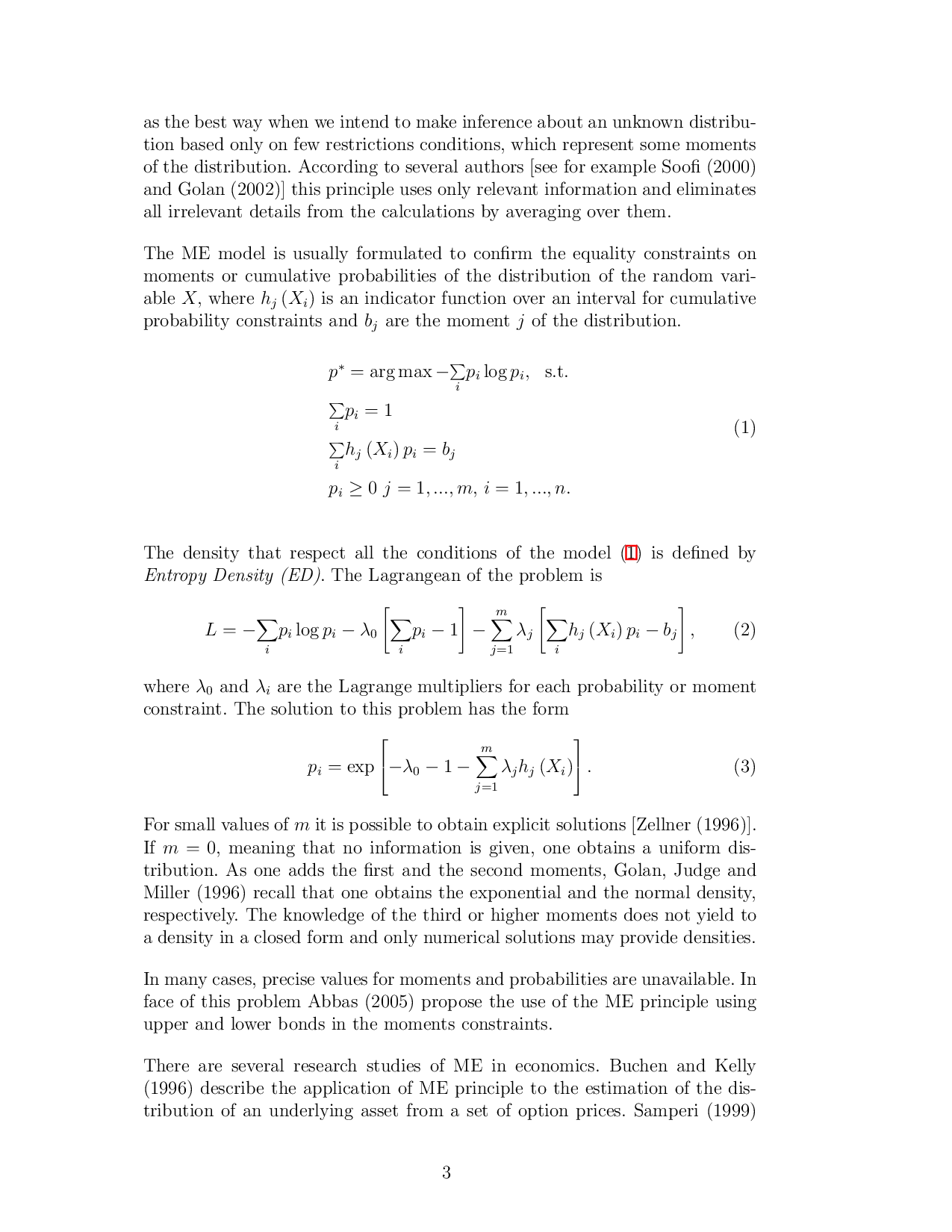
The ME model is usually formulated to confirm the equality constraints on moments or cumulative probabilities of the distribution of the random variable X, where h j (X i ) is an indicator function over an interval for cumulative probability constraints and b j are the moment j of the distribution.
The density that respect all the conditions of the model ( 1) is defined by Entropy Density (ED). The Lagrangean of the problem is
where λ 0 and λ i are the Lagrange multipliers for each probability or moment constraint. The solution to this problem has the form
For small values of m it is possible to obtain explicit solutions [Zellner (1996)].
If m = 0, meaning that no information is given, one obtains a uniform distribution. As one adds the first and the second moments, Golan, Judge and Miller (1996) recall that one obtains the exponential and the normal density, respectively. The knowledge of the third or higher moments does not yield to a density in a closed form and only numerical solutions may provide densities.
In many cases, precise values for moments and probabilitie
…(Full text truncated)…
This content is AI-processed based on ArXiv data.