Chaplygin ball over a fixed sphere: explicit integration

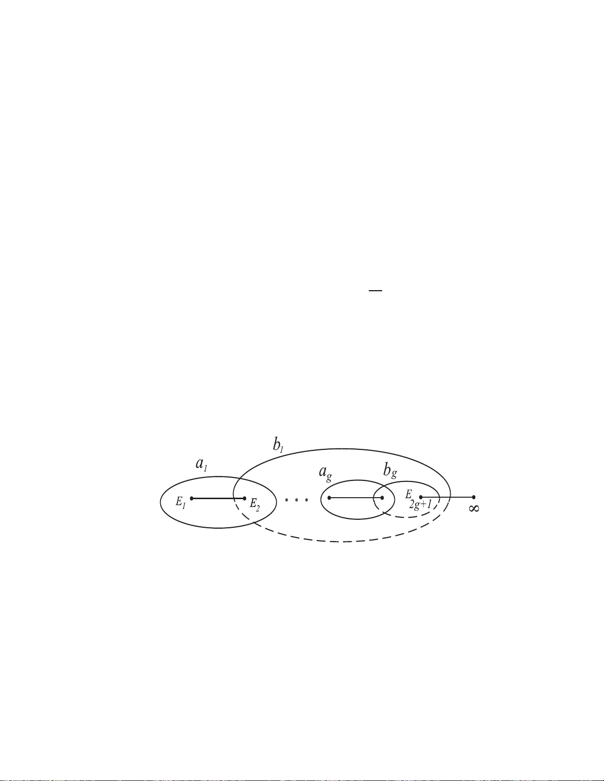
Chaplygin ball o v er a fixed sphere: explicit i n tegration ∗ A. V. Boriso v Institute of Computer Science, Udm urt State Univ ersit y , ul. Univers itetsk ay a 1, Izhevsk , 426034 Russia e-mail: borisov@rcd.ru and Y u. N. F edoro v Departmen t de Matem` atica I, Univ ersitat Politecnica de Catalun ya, Barcelona, E-08028 Spain e-mail: Yuri.Fedo rov@upc.edu and I. S. Mamaev Institute of Computer Science, Udm urt State Univ ersit y , ul. Univers itetsk ay a 1, Izhevsk , 426034 Russia e-mail: mamaev@rc d.ru Abstract W e conside r a nonholono mic system desc ribing a ro lling of a dynamically non- symmetric sphere over a fixed s pher e without slipping . The system gener alizes the classical n onholonomic Chaplygin sphere problem a nd it is shown to b e integrable for one sp ecia l ra tio of ra dii of the spheres. After a time r eparameter ization the system bec omes a Hamiltonian one and admits a separation of v a riables a nd r eduction to Ab el– Jacobi quadratures. The separating v ariables that we found app ear to b e a no n-trivial generaliza tion of ellipsoidal (sphero co nic) co ordinates on the Poisson sphere, whic h can be useful in other integrable problems. Using the qua dratures we also p erfo r m an ex plic it integration of the problem in theta-functions of the new time. 1 In tro duction One of the bes t known integrable s y stems of the cla ssical nonholonomic mechanics is the Cha plygin pr oblem on a non-homog eneous sphere rolling ov er a ho r izontal pla ne without slipping. In [8] S. A. Chaplygin obtained the equations of motion, prov ed their integrabilit y and p erformed their r e duction to qua dratures b y using spher o conical co ordinates on the Poisson spher e a s s e parating v ariables . He a lso actually solved the reconstructio n problem b y describing the motion of the spher e on the plane. V arious asp e cts of this celebrated system w er e studied in [4, 19, 8, 20], and its explicit int egration in terms of theta- functions was pr e sented in [17]. ∗ AMS Sub ject Classification 37J60, 37J35, 70H45 1 Several nontrivial integrable g e neralizations of this pro blem w ere indica ted by V. Kozlov [21] (the motion o f the sphere in a quadratic p otential fie ld), A. Markeev [23] (the spher e carr ies a rotato r ), in [25] (a n extra nonholo nomic cons traint is added) and in [15] (the sphere touches an arbitrary n um ber o f s ymmetric spheres with fixed centers). Next, among st others, the pap ers [3, 4, 26] co nsidered ro lling o f the Cha plygin (i.e., dynamically no n-symmetric) spher e ov er a fixed sphere, so called spher e-spher e pr oblem . They studied the equa tions o f motion in the frame attached to the b o dy . More g eneric (although more tedious) form of the equations also app eare d in the works of W or onetz [27, 28], who, nevertheless, solved a series of interesting pr oblems describing rolling of bo die s of revolution o r flat bo dies ov er a sphere. A rolling of a g eneric conv ex bo dy ov er a s phere was also discussed in the r e cent survey [5]. In [3, 4, 26] it was observed that the equations of motion o f the Chaplygin sphere- sphere pr oblem admit an in v ariant mea sure, but, as n umer ical computations show, in the g eneral case they are not integrable (there is no analo g of the linear momen tum int egral). How ever, as was a lso found in [3], for one s pec ia l ra tio of r adii of the t wo spheres an analog of such an in tegral do es exist, a nd the s y stem in integrable by the Jacobi last multiplier theorem. Un til recently , no o ne of the ab ov e gener alizations was integrated in quadra tur es (except a ca se of particular initial conditions of the Kolz ov genera lization, c o nsidered in [14]). In this connection it should b e noted that a Lax pair with a sp ectral par ameter fo r the Chaplyg in sphere pro blem or for its generaliz a tions is still unknown and, pr obably do es not exists. Hence, o ne cannot use the pow erful method of Baker–Akhieser functions to find theta-function solution of the problem. Con t en ts of the pap er. Our main purp os e is to find appropr iate s eparating v ari- ables, which a llow to reduce the integrable case of the Chaply g in s phere-sphere problem to quadra tures, a s well as to give explicit theta-function solution. It app ears that, in co ntrast to the classica l Chaplyg in spher e problem, the usual sphero conica l co ordinates on the Poisson s pher e do not provide separating v ar iables and that such v a riables should b e introduce d in a more complicated way (see formulas (3.2)). Using the quadra tures, w e also give a brief analysis of p ossible bifurcatio ns and per io dic solutions . These results ar e pr esented in Sections 3-4 . In Section 5 we br iefly describ e another type of p erio dic solutions. Section 6 provides a deriv ation of explicit theta-function solutions of the pro blem in a self-contained for m (Theo rem 6.4). Finally , in App endix we show how the separating v a riables we used ca n be obtained in a s ystematic w ay , by reducing a restriction o f our system to an integrable Hamilto- nian sys tem with 2 degrees of fr eedom and a pplying a cla ssical res ult of Eisenhar t on transformatio n of the Hamiltonian to a St¨ ack el form. 2 Equations of motion and first in tegrals Consider r olling of the Chaplygin spher e inside/over a fix e d sphere witho ut slipping (Figure 1.) Let ω , m , I = diag( I 1 , I 2 , I 3 ), and b denote r esp ectively the angular velocity vector of the Chaplyg in s phere, the mass of the spher e , its inertia tensor, and the r a dius. 2 By n we denote the unit normal vector to the fixed sphere S 2 at the contact p oint P . The angular momentum M of the moving sphere with r esp ect to P can b e written as M = I ω + d n × ( n × ω ) , d = mb 2 , (2.1) where × denots the vector pro duct in R 3 . The phase space o f the dyna mical system is the tangent bundle T ( S O (3 ) × S 2 ). By using the no slip no nholonomic cons traint (which corr e s po nds to zero veloc it y in the po int of contact), one can obtain the r educed equations of motion in the frame attached to the spher e in the following closed form (see, e .g ., [3]): ˙ M = M × ω , ˙ n = k n × ω , k = a a + b , (2.2) a b eing the r adius o f the fixed sphere. Note that the r atio k can take any positive or nega tive v alue dep ending o n the relative p ositio n of the rolling and fixed spheres , as illus tr ated in Fig. 1. a n b a y r b n a n b a) 0< <1 k b) k >1 c) k <0 Figure 2.1: Roll ing of the Chaplygin sphere inside/o ver the fi xed sphere (dashed). F or arbitra ry k the equations (2.2) p ossess three indep endent in tegrals F 0 = h n , n i = 1 , H = h M , ω i , F 1 = h M , M i , (2.3) which, in vie w o f (2.1), can b e wr itten as F 0 = h n , n i = 1 , H = h ω , J ω i − d 2 h n , ω i 2 , F 1 = h J ω , J ω i − 2 h J ω , n i h n , ω i + d 2 h n , ω i 2 , (2.4) where J = I + d E , E b eing the ide ntit y matrix. 3 As shown in [26], the equa tions (2.2) expressed in terms of omeg a, n also have the inv ariant mea sure ρ d ω d n with the density ρ = p h n , n i − d h n , J − 1 n i . (2.5) Thu s, a ccording to the J acobi theo r em, for a co mplete integrability of this s ystem one extra integral is needed. The Chaplygin sphere on the plane. Clearly , the ca se k = 1 corr esp onds to a → ∞ , that is, the fixed sphere transfor ms to a horizontal plane with the unit normal vector n , a nd we arr ive at the cla s sical integrable Chaply g in problem, when the linea r (in M ) moment um integral is pr eserved: h M , n i ≡ h I ω , n i . (2.6) Second integrable case. According to [3], the system (2.2) is a ls o integrable in the case k = − 1, which describ es rolling of a non-homo geneous ball with a spherical cavit y ov er a fixed sphere and the quotient of the radii of the s pheres equals b a = 1 2 (see Fig. 1 c ). In this case, instead o f (2.6), there is the following linear integral 1 F 2 = h A M , n i , (2.7) where A = diag( J 2 + J 3 − J 1 , J 3 + J 1 − J 2 , J 1 + J 2 − J 3 ) . Note that, a s w as shown in [6], the mo difica tion of this sy stem o btained by imp o sing the extra “no t wist” cons traint h ω , n i = 0 (sometimes called as the rubb er Chap lygin b al l ) is also integrable for the ratio k = − 1. In the next sec tions we pres en t explicit integration o f this case under the condition F 2 = 0. Our pro cedur e is similar to that o f the pr oblem o f the Chaplygin sphere rolling on a horizo n tal pla ne in the cas e of zero v alue of the ar ea integral (2.6), (se e [8, 19, 7]), how ever, ana ly tically , it is more complica ted. Int egration of the system (2.2) with k = − 1 in the gene r al case F 2 6 = 0 is still an op en problem. A remark on reduction to quadratures in the case d = 0 . Note that in the limit case d = 0 one has M = I ω and the equations (2.2) with k = − 1 take the form I ˙ ω = I ω × ω , ˙ n = − n × ω . As was noticed in [3 ], b y the substitution M = AI ω , γ = n (2.8) and the s ig n change t → − t , the latter system transforms to the E ule r –Poisson eq uations for the classica l Euler top, ˙ M = M × ω , ˙ γ = γ × ω , (2.9) ω i = a i M i , a i = 1 ( J j + J k − J i ) J i , (2.10) 1 W e could not interpret this integral as a momentum conserv ation law. 4 which p osses ses fir st in teg rals h M , γ i = g , h M , AM i = h, h M , M i = f , where A = diag (a 1 , a 2 , a 3 ). As was indicated in several publications (see, e .g ., [16]), the Euler – Poisson equatio ns (2.9) can b e in tegrated by sepa ration of v ariables . Namely , by an appropr iate c hoice of the co nstant vector γ in space we can always s e t g = 0. Then h A ω , γ i = 0, and the equa tions (2.9) r educe to a flow on the tangent bundle of the Poisson sphere S 2 = {h γ , γ i = 1 } . In the sphero conical co ordinates λ 1 , λ 2 on S 2 such that γ 2 i = ( a i − λ 1 )( a i − λ 2 ) ( a i − a j )( a i − a k ) , i 6 = j 6 = k 6 = i, (2.11) the flow is r educed to the quadrature s dλ 1 p R ( λ 1 ) + dλ 2 p R ( λ 2 ) = 0 , λ 1 dλ 1 p R ( λ 1 ) + λ 2 dλ 2 p R ( λ 2 ) = C dt, C = const , (2.12) R ( λ ) = − ( λ − a 1 )( λ − a 2 )( λ − a 3 )( f λ − h ) . The latter c o nt ain one holo mo rphic and one meromorphic different ial on the elliptic curve E = { µ 2 = R ( λ ) } . Thus the the quadrature s give rise to a gener alized Ab el–Ja cobi map and, following the metho ds developed in [1 0], they ca n b e inv er ted to express the v ariables γ , ω in terms of theta- functions of E and exp onents (see, e.g ., [18, 16] for the concrete expres s ions). Apparently , in the genera l ca se d 6 = 0 the s ubs titution (2.8) is not us e ful to integrate the the equations (2.2) in the se cond in tegrable case k = − 1. In par ticular, it do es not transform these equations to the case o f the cla ssical C ha plygin sphere pr oblem ( k = 1). 3 Reduction to quadratures in the case F 2 = 0 W e now consider the ca s e d 6 = 0, but assume that the linear integral F 2 in (2 .7) is zero, which imp oses restrictio ns of the initial conditions. Then, from (2.2) with k = − 1 and F 2 = 0 we get ˙ n = − n × ω , h ω , B n i = 0 , where B = ( J − d n ⊗ n ) A . This allows to express the ang ular velocity in terms of ˙ n , n in the following homogeneous fo r m ω = B n × ˙ n h n , B n i . (3.1) In view of the ab ov e remar k on the reduction to q uadratures in the case d = 0, to per form separ ation of v ariables it se ems natural to us e the sphero co nical co ordinates λ 1 , λ 2 given b y (2.11) (with γ i replaced b y n i ) in the gener a l cas e d 6 = 0 to o . How ever, this choice do es not lead to success: a fter some calculations one can see that the first int egrals H , F 1 hav e mixed terms in the der iv atives ˙ λ 1 , ˙ λ 2 . It app ear s that a corr ect choice is g iven b y the following quasi-spher o c onic al co ordi- nates z 1 , z 2 on the Poisson sphere h n , n i = 1: n 2 i = 1 G ( z 1 , z 2 ) det I ( J i − d ) J j J k ( a i − z 1 )( a i − z 2 ) ( a i − a j )( a i − a k ) , ( i, j, k ) = (1 , 2 , 3 ) , (3.2) 5 where G ( z 1 , z 2 ) = 1 − d (T r J − 2 d )( z 1 + z 2 ) + d (4 det J − d T r( JA )) z 1 z 2 , (3.3) and, as in (2.10), a i = ( A i J i ) − 1 . A systematic deriv atio n o f the substitution (3.2) is presented in App endix. Note that when d = 0, the factor G b ecomes 1 and the relation (3.2) takes the form of (2.11), tha t is, z 1 , z 2 do bec ome the usual spher o conical co ordinates on S 2 . W e note that similar quasi-spher o conical co ordinates w ere alr eady used in [6, 5] to int egrate the ”r ubbe r ” Cha plygin sphere-spher e pro blem. In the ab ov e co o r dinates z 1 , z 2 one has ρ 2 = h ( I n , J − 1 n i = det I det J 1 G ( z 1 , z 2 ) , h n , B n i = det I det A z 1 z 2 G ( z 1 , z 2 ) (3.4) and ˙ n i = 1 2 ˙ z 1 z 1 − a i + ˙ z 2 z 2 − a i − ˙ G ( z 1 , z 2 ) G ( z 1 , z 2 ) ! n i . (3.5) Then the expres sions (3.1) yield ω i = n j n k 2 J j − J k J i − d " (1 − dA i z 2 ) ˙ z 1 (1 − a − 1 j z 1 )(1 − a − 1 k z 1 ) z 2 + (1 − dA i z 1 ) ˙ z 2 (1 − a − 1 j z 2 )(1 − a − 1 k z 2 ) z 1 # , (3.6) h ω , n i = n 1 n 2 n 3 ( J 1 − J 2 )( J 2 − J 3 )( J 3 − J 1 ) G ( z 1 , z 2 ) 2 det I  ˙ z 1 Φ( z 1 ) z 2 + ˙ z 2 Φ( z 2 ) z 1  , (3 .7) Φ( z ) = ( a − 1 1 z − 1)( a − 1 2 z − 1)( a − 1 3 z − 1) . Substituting them, as well as (3.2), into the integrals H , F 1 in (2.4), after simplificatio ns we get H = ( z 1 − z 2 ) det I 4 G 2 ( z 1 , z 2 )  Ψ( z 2 ) Φ( z 1 ) z 2 2 ˙ z 2 1 − Ψ( z 1 ) Φ( z 2 ) z 2 1 ˙ z 2 2  , F 1 = ( z 1 − z 2 ) det I 4 G 2 ( z 1 , z 2 )  ψ ( z 2 ) Φ( z 1 ) z 2 2 ˙ z 2 1 − ψ ( z 1 ) Φ( z 2 ) z 2 1 ˙ z 2 2  (3.8) where Ψ( z ) = d det A z 2 − T r( AJ ) z + 2 , ψ ( z ) = (4 det J − d T r( AJ )) z − (T r J − 2 d ) . (3.9) Next, substituting (3.6), (3.7), and (3.2) into (2.1), we also o btain M i = n j n k 2 ( J k − J j ) " ˙ z 1 (1 − a − 1 j z 1 )(1 − a − 1 k z 1 ) z 2 + ˙ z 2 (1 − a − 1 j z 2 )(1 − a − 1 k z 2 ) z 1 # . (3.10) Now, fixing the v alues of the in teg rals by setting H = h, F 1 = f , then solv ing (3.8) with resp ect to ˙ z 2 1 , ˙ z 2 2 and using the relation Ψ( z 2 ) ψ ( z 1 ) − Ψ( z 1 ) ψ ( z 2 ) = det A ( z 2 − z 1 ) G ( z 1 , z 2 ) , (3.11) we get ˙ z 2 α = − z 2 β G ( z 1 , z 2 ) ( z 1 − z 2 ) 2 4Φ( z α )( f Ψ ( z α ) + hψ ( z α )) det I det A = − z 2 β G ( z 1 , z 2 ) ( z 1 − z 2 ) 2 4( z α − a 1 )( z α − a 2 )( z α − a 3 ) ( f Ψ( z α ) + hψ ( z α )) , ( α, β = (1 , 2) . 6 After the time repa rameterizatio n dt = 1 p G ( z 1 , z 2 ) dτ ≡ r det J det I h I n , J − 1 n i dτ (3.12) the ab ov e relations g ive dz 1 dτ = z 2 p R ( z 1 ) z 1 − z 2 , dz 2 dτ = z 1 p R ( z 2 ) z 2 − z 1 , (3.13) R ( z ) = − ( z − a 1 )( z − a 2 )( z − a 3 ) ( f Ψ( z ) + hψ ( z )) . The latter are eq uiv a lent to the following Ab el–Ja cobi t yp e quadra tures dz 1 p R ( z 1 ) + dz 2 p R ( z 2 ) = 2 dτ , z 1 dz 1 p R ( z 1 ) + z 2 dz 2 p R ( z 2 ) = 0 , (3.14) which contain 2 holomorphic differentials on the hyperelliptic genus 2 curve Γ = { w 2 = R ( z ) } . In view of (3 .9) , when d → 0 , the po lynomial R ( z ) b ecomes a deg ree 4 p o ly nomial, and (3.14) re duce to the quadratures (2.12) for the E uler top problem, as exp ected. It is interesting tha t, like in the in tegration of the original Chaply gin s phere pro blem presented in [8], the r eparameter iz ation factor in (3.12) co incide s with the density (2.5) of the inv ariant measure. In the real motion this factor never v anishes, hence the repara meter ization is no n-singular. Now substituting the above formulas for ˙ z 2 1 , ˙ z 2 2 int o (3.10), (3.6) and simplifying , we expr ess the ang ular momen tum M and the velocity ω in terms of z 1 , z 2 and the conjugated co ordina tes w 1 , w 2 : M i = p I j I k I i p ( J i − J j )( J i − J k ) p ( a j − z 1 )( a j − z 2 ) p ( a k − z 1 )( a k − z 2 ) 2 p G ( z 1 , z 2 ) × 1 z 1 − z 2  w 1 ( z 1 − a j )( z 1 − a k ) − w 2 ( z 2 − a j )( z 2 − a k )  . (3.15) ω i = p I j I k p ( J i − J j )( J i − J k ) p ( a j − z 1 )( a j − z 2 ) p ( a k − z 1 )( a k − z 2 ) 2 p G ( z 1 , z 2 ) × 1 z 1 − z 2  ( z 2 − 1 / ( dA i ) w 1 ( z 1 − a j )( z 1 − a k ) − ( z 1 − 1 / ( dA i )) w 2 ( z 2 − a j )( z 2 − a k )  . (3.16) Next, the pro jection h ω , n i in (3 .7) ta kes the form h ω , n i = J 1 J 2 J 3 p ( z 1 − a 1 )( z 1 − a 2 )( z 1 − a 3 ) ( z 2 − a 1 )( z 2 − a 2 )( z 2 − a 3 ) × 1 z 1 − z 2  w 1 ( z 1 − a 1 )( z 1 − a 2 )( z 1 − a 3 ) − w 2 ( z 2 − a 1 )( z 2 − a 2 )( z 2 − a 3 )  . Since w α = p − ( z α − a 1 )( z α − a 2 )( z α − a 3 ) ( f Ψ( z α ) + hψ ( z α )) = p − ( z α − a 1 )( z α − a 2 )( z α − a 3 ) f d det A ( z α − c 1 )( z α − c 2 ) , the latter relatio n a lso reads h ω , n i = J 1 J 2 J 3 p ( c 1 − z 1 )( c 1 − z 2 ) p ( c 2 − z 1 )( c 2 − z 2 ) × − 1 z 1 − z 2  w 1 ( z 1 − c 1 )( z 1 − c 2 ) − w 2 ( z 2 − c 1 )( z 2 − c 2 )  . (3.17) In Section 6 we shall use the above ex pressions to obtain explicit theta-function solutions for the co mp onents of n, ω , M in terms o f the new time τ . 7 4 Qualitativ e study of the motion and b ifurcations F or generic consta n ts h, f the p olyno mia l R ( z ) in (3.14) has simple ro ots a i , c 1 , c 2 , and in the r eal motion the sepa rating v ariables z 1 , z 2 evolv e b etw een them in such a wa y that R ( z 1 ) , R ( z 2 ) remain non-negative. This co r resp onds to a qua sip erio dic motion o f the sphere. In the sequel we a ssume that the moments o f inertia I 1 , I 2 , I 3 corres p o nds to a ph ysical rig id bo dy , i.e., that the triangula r ineq ualities I i + I j > I k are satisfies . F or concreteness, as sume also that d < J 1 < J 2 < J 3 . This als o implies 0 < A 3 < A 2 < A 1 and 0 < a 1 < a 2 < a 3 . As follows from the first expr ession in (3.4), in the real case the factor G ( z 1 , z 2 ) is alwa ys positive. Hence, the right hand sides of (3.2) a re p ositive and the co ordina tes n i are rea l and satisfy h n , n i = 1 if a nd only if z 1 ∈ [ a 1 , a 2 ] and z 2 ∈ [ a 2 , a 3 ], like the usual sphero conical co or dinates. Next, we hav e Prop ositio n 4. 1. F or the r e al motion, when t he c onst ants h, f ar e p ositive, and for any d, J i satisfying the ab ove ine qualities, the r o ots c 1 ≤ c 2 never c oincide and c 1 < a 1 and if f /h = J i , then c 1 = 2 d − A i d A k A j < a 1 , c 2 = a i . Pr o of. Set f /h = λ ∈ R . The ro o ts c 1 , c 2 coincide with those of Ψ ( z ) λ + ψ ( z ) and hav e the form c 1 , 2 = T r( AJ )( λ + d ) ± √ D d det A , (4.1) D = (T r( AJ )) 2 ( λ + d ) 2 − 8 d det A ( λ + d ) + 4 d det A T r J . The condition D = 0 gives a qua dratic equation on λ , whose determinant equa ls − d det I det A 2 , alwa ys a negative num b er . Hence D > 0 a nd c 1 < c 2 . Next, in v iew of (4.1), the condition c 1 − a 1 = 0 also leads to a q ua dratic equation for λ , a gain with always negative deter minant . Then, ev a luating c 1 − a 1 for one v a lue of λ , we find c 1 < a 1 for any λ ∈ R . Finally , setting in (4.1 ) λ = J i and s implifying, we obtain the indica ted ab ov e expressions for c 1 , c 2 . Combining the statement of Prop ositio n 4.1 with the p er mitted p o s itions o f z 1 , z 2 , we conclude that, depending on v alue of c 2 , z 1 ∈ [ a 1 , c 2 ] , z 2 ∈ [ a 2 , a 3 ] , or z 1 ∈ [ a 1 , a 2 ] , z 2 ∈ [ c 2 , a 3 ] . (4.2) Then, in view of (3.2), the vector n alwa ys fills a ring R o n the unit sphere S 2 = {h x, x i = 1 } be t ween the lines o f its in tersection with the co ne 3 X i =1 J i − d J i x 2 i a i − c 2 = 0 . P erio dic solutions with bifurcations. As follows fr om Prop osition 4.1, the only p erio dic solutions with bifurcations ca n occ ur when the root c 2 coincides with a 1 , a 2 or a 3 2 . This happe ns under the initial co nditions ω i = ω j = 0 , n k = 0 , ( i, j, k ) = (1 , 2 , 3) , 2 There is another type of p eriodic solutions correspond ing to p eriod ic wind in gs of th e 2-dimensional tori. How ever, th e latter are n ot related to b ifurcations and we d o not consider them here. 8 when the spher e p er forms a p erio dic circula r motion with n k ≡ 0 and one has h ω , n i ≡ 0, H = J k ω k , F 1 = J 2 k ω 2 k , which y ields f / h = J k . Then, in view of the ab ov e prop osition, c 2 = a k and the p olynomial R ( z ) in (3.1 3) has the double ro ot a k , as exp ected. When λ = f /h leaves the interv al [ J 1 , J 3 ], the ro ot c 2 go es b eyond o f [ a 1 , a 3 ]. Then for R ( z 1 ) , R ( z 2 ) to b e bo th p ositive, one of z i m ust violate the co nditio n (4.2). This implies that in the real case the quotient f /h b elong s to [ J 1 , J 3 ], and the bifurcation diagram on the pla ne ( h, f ) consists o nly of 3 rays f /h = J 1 , J 2 , J 3 . Note that, ac c o rding to the results of [8], a similar situation takes place for the Chaplygin sphere on the horizontal plane. The motion of the con tact p oint on the fixed sphere. As mentioned ab ov e, in the generic case with F 2 = 0 the co ntact p oint on the mo ving sphere given by the vector n b elongs to the ring R on S 2 . Then the fo llowing na tur al question arises: do es t he c ont act p oint on the fixe d spher e also b elongs to a ring or it c over the whole spher e ? (Recall ([8]) that in the ca se of the Chaplygin sphere on a ho rizontal plane the contact p oint o n the plane mov es inside a strip, whose a x is is orthogona l to the hor izontal momentu m vector.) T o study the ab ov e problem we assume, without lo s s o f generality , that the r adius a of the fixed spher e is 1. Then the contact point on this sphere is given by the unit vector n as viewed in sp ac e . T o describ e the spatial evolution of n , intro duce a fixed or thogonal frame O ξ η ζ with the c e n ter O in the center o f the fixed spher e and the “vertical” ax is O ζ directed along the fixed momentum vector M . Then, in view of (3.10), the pro jection of n o n Oζ can be written in form n ζ = 1 | M | h n , M i = 1 √ f a 1 a 2 a 3 ( J 1 − J 2 )( J 2 − J 3 )( J 3 − J 1 ) n 1 n 2 n 3 ×  z 1 ˙ z 1 ( z 1 − a 1 )( z 1 − a 2 )( z 1 − a 3 ) z 2 + z 2 ˙ z 2 ( z 2 − a 1 )( z 1 − a 2 )( z 1 − a 3 ) z 1  , which, following (3.2) and the expr essions for ˙ z 2 1 , ˙ z 2 2 , after a simplification, reads n ζ = √ − 1 √ f J 1 J 2 J 3 p ( c 1 − z 1 )( c 1 − z 2 ) p ( c 2 − z 1 )( c 2 − z 2 ) × 1 G ( z 1 , z 2 ) − 1 z 1 − z 2  z 2 w 1 ( z 1 − c 1 )( z 1 − c 2 ) − z 1 w 2 ( z 2 − c 1 )( z 2 − c 2 )  . (4.3) It follows that the r ight hand side of (4.3) is a quasip erio dic function of time. One can show that under the co nditions (4.2) and c 1 < a 1 < a 2 < a 3 , the function n ζ ( z 1 , w 1 , z 2 , w 2 ) is real a nd, regar dless to signs o f the r o ots w α = p R ( z α ), the function | n ζ | has the abso lute ma ximum in o ne o f the vertices of the quadrang le Q ⊂ ( z 1 , z 2 ) = R 2 defined by (4.2). In tw o other vertices of Q this function is zero . Calculating | n ζ | in the vertices of Q , we find that for c 2 6 = a i its maximum is str ictly less than 1 . It follows that the tr a jectory n ( t ) on the fixed spher e lies b etw een the “horizontal” planes ζ = ± ν , ν < 1 . T o describ e the tr a jectory n ( t ) on the fixed sphere in the “ longitudinal” dir ection, apart fr om the fixed momentum vector M it is go o d to know another fixed vector which can b e e x pressed in terms of ω , n . Howev er, it seems that such a vector do es not exist, and for this reas on we intro duce the longitude angle ψ b et ween the axis O ξ and the vertical plane spanned by M and n . In tro duce a lso the the longitudinal unit vector 9 u = M × n / | M × n | . The n we find ˙ ψ = | M | | M × n |  u , d dt n  = | M |  M × n , d dt n  h M × n , M × n i , where d dt n is the absolute deriv ative of n ex pr essed in the co ordinates of the moving frame. In view of the second vector e q uation in (2.1) with k = − 1, d dt n = ˙ n + ω × n = 2 ω × n . Hence, we get ˙ ψ = | M | h M × n , 2 ω × n i h M × n , M × n i . (4.4) Next, using the expressions (3 .6), (3.10), we o btain 2( ω × n ) i = n i ( J i − d ) G  dA j A k z 2 + A i − 2 d a − 1 i z 1 − 1 ˙ z 1 + dA j A k z 1 + A i − 2 d a − 1 i z 2 − 1 ˙ z 2  , ( M × n ) i = n i ( J i − d ) 2 G  (2 J j J k − dA i ) z 2 − 1 ( a − 1 i z 1 − 1) z 2 ˙ z 1 + (2 J j J k − dA i ) z 1 − 1 ( a − 1 i z 2 − 1) z 1 ˙ z 2  , ( i, j, k ) = (1 , 2 , 3 ) . Substituting these formulas into (4 .4) and expressing the deriv atives ˙ z α in terms of z 1 , w 1 , z 2 , w 2 , one finds the deriv ative ˙ ψ as a symmetric function of ( z 1 , w 1 ) and ( z 2 , w 2 ), that is, as a q ua sip erio dic function of t . Its in tegration yields ψ ( t ), which, together with (4.3), provides a co mplete description of the co ntact po in t on the fixed spher e. 5 A sp ecial case of p erio dic motion. Apart fr om the par ticular cas e of the mo tion with F 2 = 0, there is another sp ecia l case, when this integral takes the max imal v alue, that is, when A n is parallel to the momentum vector M . In this ca se M = h A n , h = const. In view of (2.1), this implies J ω − d h ω , n i = h A n and ω = h J − 1  A n + d ρ 2 h A n , J − 1 n i  , (5.1) ρ b eing the s a me as in (2.5). Substituting the express ion for ω in to the s econd equation in (2.2) and simplifying, we get the following c losed system for n : n = h J 1 + J 2 + J 3 − 2 d F ( n × J − 1 n ) . (5.2) It has tw o indep endent integrals h n , n i a nd h n , J − 1 n i o r h A n , A n i , which implies that the factor F is cons ta n t on the tra jectories and that the sy stem ha s the form of the Euler top equa tions. As a res ult, in the general case the comp onents of n and ω are expressed in terms of elliptic functions of the or iginal time t a nd their evolution is per io dic. This situation is similar to that of the sp ecial c ase of the motion of the Chaplygin sphere on a horizo n tal plane, when the momentum vector M is vertical, and when the solutions are elliptic in the origina l time. 10 6 Theta-function solutions in the case F 2 = 0 . In o rder to find e xplicit so lutions for the comp onents of ω , M , n , and other v ariables, we first remind some necessa ry bas ic facts on the Jacobi inv er sion pro blem a nd its s olution. Solving the Ja cobi in version problem by means of W urzelfunktionen. Consider a n o dd-or der genus g hyperelliptic Riemann sur face Γ obta ined from the affine curve { µ 2 = R ( λ ) } , R ( λ ) = ( λ − E 1 ) · · · ( λ − E 2 g +1 ) } , by adding one infinite p oint ∞ . Let us cho o se a canonical bas is of cycles a 1 , . . . , a g , b 1 , . . . , b g on Γ such that a i ◦ a j = b i ◦ b j = 0 , a i ◦ b j = δ ij , i, j = 1 , . . . , g , where γ 1 ◦ γ 2 denotes the in tersection index of the cycles γ 1 , γ 2 (F or r eal br anch p oints see an example in Figure 6.1). Next, let ¯ ω 1 , . . . , ¯ ω g be the conjuga ted basis of nor malized holomorphic differentials on Γ such that I a j ¯ ω i = 2 π  δ ij ,  = √ − 1 . The g × g matrix o f b -p erio ds B ij = H b j ¯ ω i is symmetric and has a nega tive de finite real part. Conside r the p e r io d lattice Λ 0 = { 2 π  Z g + B Z g } of rank 2 g in C g = ( Z 1 , . . . , Z g ). The complex torus Jac(Γ) = C g / Λ 0 is called the Jac obi v ar iet y ( Jac obian ) o f the curve Γ. F o r a fixed p oint P 0 the Ab e l map A : Γ 7→ Jac(Γ) , A ( P ) = Z P P 0 ( ¯ ω 1 , . . . , ¯ ω g ) T describ es a natural embedding of the curve into its J acobian. Figure 6.1: A canonical b asis of cycles on the hyperelliptic cu rve represented as 2-fold co vering of the complex plane λ . The p arts on the cycles on the lo wer sheet are sho wn by dashed lines. Now cons ider a generic diviso r of p oints P 1 = ( λ 1 , µ 1 ) , . . . , P g = ( λ g , µ g ) on it, and the Ab e l– Jacobi mapping with a ba sep oint P 0 Z P 1 P 0 ¯ ω + · · · + Z P g P 0 ¯ ω = Z , (6.1) ¯ ω = ( ¯ ω 1 , . . . , ¯ ω g ) T , Z = ( Z 1 , . . . , Z g ) T ∈ C g . 11 Under the mapping, symmetric functions of the co o rdinates of the p oints P 1 , . . . , P g are 2 g -fo ld p erio dic functions of the complex v a riables Z 1 , . . . , Z g with the ab ov e p erio d lattice Λ 0 (Abelian functions). Explicit expressions of such functions can be obtained by means of theta-functions on the universal cov er ing C g = ( Z 1 , . . . , Z g ) o f the complex tor us. Recall that customary Riemann’s theta -function θ ( Z | B ) asso cia ted with the Riemann matrix B is defined by the series 3 θ ( Z | B ) = X M ∈ Z g exp hh B M , M i + h M , Z i ) , (6.2) h M , Z i = g X i =1 M i Z i , h B M , M i = g X i,j =1 B ij M i M j . Equation θ ( Z | B ) = 0 defines a co dimension one subv ar iety Θ ∈ Jac(Γ) (for g > 2 with singularities ) ca lled theta-divisor . W e shall also use t heta-fun ctions with char acteristics α = ( α 1 , . . . , α g ) , β = ( β 1 , . . . , β g ) , α j , β j ∈ R , which are obtaine d from θ ( Z | B ) b y shifting the arg ument Z and mult iplying b y an exp onent 4 : θ  α β  ( Z ) ≡ θ  α 1 · · · α g β 1 · · · β g  ( Z ) = exp {h B α, α i / 2 + h Z + 2 π β , α i} θ ( Z + 2 π  β + B α ) . All these functions enjoy the quadip erio dic prop er t y θ  α β  ( Z + 2 π K + B M ) = exp(2 π ǫ ) exp {−h B M , M i / 2 − h M , Z i} θ  α β  ( Z ) , (6.3) ǫ = h α, K i − h β , M i , Now for a g eneric divisor P 1 = ( λ 1 , µ 1 ) , . . . , P g = ( λ g , µ g ) on Γ , in tro duce the po lynomial U ( λ, s ) = ( s − λ 1 ) · · · ( s − λ g ), λ ∈ C . It is known (see e.g ., [1, 2]) that given a g eneric constant C 6 = E i , then under the Abel mapping (6.1) with P 0 = ∞ the following rela tions ho ld U ( λ, C ) ≡ ( C − λ 1 ) · · · ( C − λ g ) = κ θ [∆]( Z − q ) θ [∆]( Z + q ) θ 2 [∆]( Z ) , (6.4) q = A ( C , p R ( C )) = Z ( C, √ R ( C )) ∞ ( ¯ ω 1 , . . . , ¯ ω g ) T , where κ is a c o nstant dep ending on the p erio ds of Γ only . These relation can b e ge ne r alized in different wa ys a s fo llows. 3 The expression for θ ( Z ) w e use here is different from th at chosen in a series of b o oks on th eta-functions by multiplication of Z by a constant factor. 4 Here and b elow we omit B in the theta-functional notation. 12 Theorem 6.1. (see , e.g., [1, 2, 1 6]). U n der the Ab el mapping (6.1) with P 0 = ∞ the fol lowing r elations hold p U ( λ, E i ) ≡ q ( E i − λ 1 ) · · · ( E i − λ g ) = k i θ [∆ + η i ]( Z ) θ [∆]( Z ) , (6.5) g X k =1 µ k Q l 6 = k ( λ k − λ l ) p U ( λ, E i ) p U ( λ, E j ) ( E i − λ k )( E j − λ k ) = k ij θ [∆ + η ij ]( Z ) θ [∆]( Z ) , (6.6) i, j = 1 , . . . , 2 g − 1 , i 6 = j, wher e k i , k ij ar e c ertain c onstants dep ending on the p erio ds of Γ only, and ∆ =  ∆ ′ ∆ ′′  , η i =  η ′ i η ′′ i  , ∆ ′ , ∆ ′′ , η ′ i , η ′′ i ∈ 1 2 Z g / Z g ar e half-inte ger theta-char acteristics such that 2 π  η ′′ i + B η ′ i = Z ( E i , 0) ∞ ¯ ω (mo d Λ) , (6.7) 2 π i ∆ ′′ + B ∆ ′ = K (mo d Λ) , and η ij = η i + η j (mo d Z 2 g ) , K ∈ C g b eing the ve ctor of the Ri emann c onstants. Apparently , r elations (6.6) were first o bta ined in the explicit form by K ¨ onigsb erger ([22]). E arlier, expressio ns (6.5) ha d b een cons idered by K.W eiers trass as gener a lizations of the Ja cobi elliptic functions s n( Z ) , cn( Z ), and dn( Z ). This s e t of rema rk able r elations betw een ro ots of certa in functions on symmetric pr o ducts of hyperelliptic curves and quotients of theta-functions with ha lf-int eger characteristics is historica lly referred to as Wurzelfunktionen (ro ot functions). One can show (se e , e.g., [13, 1]) that for the chosen c anonical basis of cy cles a 1 , . . . , a g , b 1 , . . . , b g on Γ, ∆ ′ = (1 / 2 , . . . , 1 / 2) T , ∆ ′′ = ( g / 2 , ( g − 1) / 2 , . . . , 1 , 1 / 2) T (mo d 1) . (6.8) In the ca se g = 2 , all the functions in (6 .5), (6.6) are single-v alued on the 1 6-fold cov er ing T 2 → Jac(Γ) with each of the four p erio ds of Λ 0 doubled, so that T 2 and Jac(Γ) are transfor med to e ach other by the change Z → 2 Z. In view of (6.7), (6.8), one has ∆ =  1 / 2 1 / 2 0 1 / 2  , ∆ + η 1 =  0 1 / 2 0 1 / 2  , ∆ + η 2 =  0 1 / 2 1 / 2 1 / 2  , ∆ + η 3 =  1 / 2 0 1 / 2 1 / 2  , ∆ + η 4 =  1 / 2 0 1 / 2 0  , ∆ + η 5 =  1 / 2 1 / 2 1 / 2 0  . (6.9) W e shall a lso need the following mo dificatio n of the K¨ onigsb er g er formula (6.6), which, for our c o nv enience, we adopt for the case g = 2 . Theorem 6.2. L et C ∈ C b e a c onstant that do es not c oicide with E i . Then under the Ab el mapping (6.1) with g = 2 and P 0 = ∞ : 1 λ 1 − λ 2  µ 1 ( E i − λ 1 )( E j − λ 1 )( C − λ 1 ) − µ 2 ( E i − λ 2 )( E j − λ 2 )( C − λ 2 )  = ˆ k ij θ 2 [∆]( Z ) θ [∆ + η ij ]( Z − q ) θ [∆ + η ij ]( Z + q ) θ [∆ + η i ]( Z ) θ [∆ + η j ]( Z ) θ [∆]( Z − q ) θ [∆]( Z + q ) , (6.10) i, j = 1 , . . . , 2 g − 1 , i 6 = j, 13 wher e ˆ k ij ar e c onstants dep ending on the p erio ds of Γ only and, as in (6.4) , q = A ( C, p R ( C ) ) . Pr o of. Let us fix the p oint P 2 = ( λ 2 , µ 2 ) in a generic p osition on the curve Γ a nd consider the following mer omorphic function on this cur ve f ( P ) = µ + µ 2 ( λ − E i )( λ − E j )( λ − C ) ) ( λ 2 − E i )( λ 2 − E j )( λ 2 − C ) ( λ − λ 2 )( λ − E i )( λ − E j )( λ − C ) . Due to the o rder of p oles and z eros of z , w , and λ − E i , λ − C o n Γ, for any gener ic P 2 , the function f ( P ) has simple p oles a t P = P 2 , E i , E j , Q − , Q + and do es not hav e a p ole neither at ιP 2 = ( λ 2 , − µ 2 ), nor a t any other po int on Γ . Next, f ( P ) has a double zero at ∞ . Then, using the descr iption of zero s of θ ( Z ), θ [∆ + η i ]( Z ) , θ [∆ + η ij ]( Z ) one can show that up to a co nstant factor, f ( P ) = ¯ f ( P ) w ith ¯ f ( P ) = θ 2 [∆]( A ( P ) − A ( P 2 )) θ [∆ + η i ]( A ( P ) − A ( P 2 )) θ [∆ + η j ]( A ( P ) − A ( P 2 )) × θ [∆ + η ij ]( A ( P ) − q − A ( P 2 )) θ [∆ + η ij ]( A ( P ) + q − A ( P 2 )) θ [∆]( A ( P ) − q − A ( P 2 )) θ [∆]( A ( P ) + q − A ( P 2 )) . Note that due to the quasip erio dic pro pe r ty of the theta - functions with c haracter is tics, ¯ f ( P ) is a mero morphic function on G . Now setting P = ιP 1 = ( λ 1 , − µ 1 ), the function − f ( P ) transfor ms to the left hand side of (6 .10), and the arg umen t A ( P ) − A ( P 2 ) b ecomes − Z . Hence ¯ f ( P ) transforms to the rig h t hand s ide of (6 .1 0), which prov e s the theor em. Combining Theor em 6.2 and formula (6.4 ), we o btain the following useful corollar y . Prop ositio n 6.3. Under the Ab el mapping (6.1 ) with g = 2 and P 0 = ∞ , 1 λ 1 − λ 2  ( C − λ 2 ) µ 1 ( E i − λ 1 )( E j − λ 1 ) − ( C − λ 1 ) µ 2 ( E i − λ 2 )( E j − λ 2 )  = const ij θ [∆ + η ij ]( Z − q ) θ [∆ + η ij ]( Z + q ) θ [∆ + η i ]( Z ) θ [∆ + η j ]( Z ) , (6.11) q = A ( C , p R ( C ) ) , i, j = 1 , . . . , 2 g − 1 , i 6 = j, C 6 = E i . Pr o of. Indeed, the left hand side of (6.11) is obta ined fro m that of (6.10) b y mult ipli- cation by ( C − λ 1 )( C − λ 2 ), whose theta-function express ion is given b y formula (6.4). Then the pro duct o f r ight hand sides o f (6.10) a nd (6.4) gives (6.11). Explicit theta-function solutions. Now let Γ b e the g enus 2 curve { w 2 = R ( z ) } , R ( z ) = − ( z − a 1 )( z − a 2 )( z − a 3 ) ( z − c 1 )( z − c 2 ) , c 1 < c 2 being the ro ots of f Ψ( z ) + hψ ( z ). Thus we iden tify (without or der) { E 1 , . . . , E 5 } = { a 1 , a 2 , a 3 , c 1 , c 2 } , and denote the cor resp onding half-integer characteristic η i by η a i and η c α . Next, choo se the canonic a l basis of cycles as depicted in Fig. 6.1 and calculate the 2 × 2 p erio d matr ix A ij = I a j  i ,  1 = dz p R ( z ) ,  2 = z dz p R ( z ) . 14 Then the norma lized holomorphic differentials on Γ a re ¯ ω k = 2 X j =1 C kj z j − 1 dz p R ( z ) , C = A − 1 , and the quadr atures (3.14) g ive Z ( z 1 ,w 1 ) ∞ ¯ ω 1 + Z ( z 2 ,w 2 ) ∞ ¯ ω 1 = Z 1 , Z ( z 1 ,w 1 ) ∞ ¯ ω 2 + Z ( z 2 ,w 2 ) ∞ ¯ ω 2 = Z 2 , ( 6.12) Z 1 = 2 C 11 τ + Z 10 , Z 2 = 2 C 21 τ + Z 20 , (6.13) Z 10 , Z 20 being constant phases. Now, comparing the last fr action in (3.2) with the expression (6.5 ) in Theo rem 6.1, we find S i ≡ p ( a i − z 1 )( a i − z 2 ) p ( a i − a j )( a i − a k ) = k i θ [∆ + η a i ]( Z ) θ [∆]( Z ) , ( i, j, k ) = (1 , 2 , 3 ) , (6.14) where Z = ( Z 1 , Z 2 ) and the comp onents of Z dep e nd on τ according to (6.13). T o calculate k i , we set here z 1 = a j , z 2 = a k . Then, in view o f (6.1 2), the definitio n of θ with characteristics a nd the quasip er io dic pro p er t y (6.3), 1 = k i θ [∆ + η a i ]( A ( a j ) + A ( a k )) θ [∆]( A ( a j ) + A ( a k )) = k i θ [∆](0 ) θ [∆ + η a i ](0) , that is, k i = θ [∆ + η a i ](0) θ [∆](0 ) . In order to e x press in theta-functions the factor G ( z 1 , z 2 ) given by (3.3), we fis t note that it do es not split into a pro duct of linear functions in z 1 and z 2 , hence one cannot use the formula (6.4 ). On the other hand, fro m the condition n 2 1 + n 2 2 + n 2 3 ≡ 1 we find that G = det I det J  J 1 J 1 − d S 2 1 + J 2 J 2 − d S 2 2 + J 3 J 3 − d S 2 1  , which, in vie w o f (6.14), gives p G ( z 1 , z 2 ) = r det I det J p Σ( Z ) θ [∆]( Z ) , (6.15) Σ( Z ) = J 1 I 1 θ 2 [∆ + η a 1 ]( Z ) + J 2 I 2 θ 2 [∆ + η a 2 ]( Z ) + J 3 I 3 θ 2 [∆ + η a 3 ]( Z ) . As a lo cal singula r ity analysis shows, in general the function Σ( Z ) has zeros of first order, hence it canno t b e a full squar e of another theta- function expressio n. Now, using theta-function expr essions (6.14), (6.15) in formulas (3.2), (3.15), (3.1 6) and applying also the W urzelfunktionen (6.6 ), (6.11) with C = 1 / ( dA i ), we a rrive at the following theor em. Theorem 6.4. The generic theta-function solutions for the Chap lygin spher e-spher e pr oblem in the c ase F 2 = 0 have the form n i ( τ ) = κ i θ [∆ + η a i ]( Z ) p Σ( Z ) , (6.16) M i ( τ ) = ν i θ [∆ + η a j + η a k ]( Z ) p Σ( Z ) , (6.17) ω i ( τ ) = ε i θ [∆ + η a j + η a k ]( Z − q i ) θ [∆ + η a j + η a k ]( Z + q i ) θ [∆]( Z ) · p Σ( Z ) , (6.18) q i = A (1 / ( dA i ) , p R (1 / ( dA i ))) , κ i , ν i , ε i = const , ( i, j, k ) = (1 , 2 , 3) , 15 wher e t he char acteristics ar e given in (6.9) and Z 1 , Z 2 dep end line arly on τ as describ e d in (6.13) . W e do not give explicit expressions for the consta nt s κ i , ν i , ε i here. Note that due to pr esence of the squa re r o ot, the v ariables n i , M i , ω i are not mero - morphic functions of Z 1 , Z 2 and therefore, of the new time τ . This stays in contrast with the solutions of the classica l Chaplyg in sphere problem, which, after a similar time repara meter ization, b ecome mer omorphic (see [11, 17]). Next, comparing the expres sion (3.17) with the W urzelfunktion (6 .6) a nd (4 .3) with (6.11), assuming C = 0, we als o find h ω , n i = υ θ [∆ + η c 1 + η c 2 ]( Z ) θ [∆]( Z ) , (6.19) n ζ =  θ [∆ + η c 1 + η c 2 ]( Z − ˆ q ) θ [∆ + η c 1 + η c 2 ]( Z + ˆ q ) θ [∆]( Z ) p Σ( Z ) , (6.20) ˆ q = A (0 , p R (0)) , υ ,  = const . The second for m ula, to g ether w ith (6 .13), des crib es the altitude of the contact p oint on the fixed sphere a s a function of τ . Finally , given the expr ession (6.15) for the factor G , the o r iginal time t can b e found as a function o f τ by integrating the quadrature (3.12). App endix. Separation of v ariables via reduction to a Hamiltonian system As mentioned ab ov e, the subs titution (3.2) is q uite non- trivial and can har dly b e guessed a priori. Below we describ e how one ca n obtain it in a sy s tematic w ay . A1. Reduction to a Hamiltonian system on S 2 First introduce the s phero conical co ordinates u, v o n the Poisson sphere h n , n i = 1: n 2 i = ( J i − u )( J i − v ) ( J i − J j )( J i − J k ) , i 6 = j 6 = k 6 = i, J i = I i + d. (6.21) Then, under the substitution (3.1), the equations (2.2) with k = − 1 give ris e to the following Chaplyg in-type system on S 2 d dt ∂ T ∂ ˙ u − ∂ T ∂ u = ˙ u Φ , d dt ∂ T ∂ ˙ v − ∂ T ∂ v = − ˙ v Φ , (6.22) T = 1 2 ( b uu ˙ u 2 + b uv ˙ u ˙ v + b vv ˙ v 2 ) , Φ = ( a u ˙ u + a v ˙ v ) , where T is the e ne r gy integral (2.3) expressed in the sphero co nic a l co ordinates under the condition F 2 = 0 a nd Φ is linear homog eneous in ˙ u, ˙ v . Explicit expressio ns for the co efficients of T , Φ a re q uite tedious, so we do not give them her e. Int ro ducing the momenta P u = ∂ T ∂ ˙ u , P v = ∂ T ∂ ˙ v , this system can b e transfo r med to a Hamiltonian fo rm with ex tra terms, which p oss esses inv a riant measure N du dv dP u dP v with the density N = 2 uv + ( u + v )(2 d + α 1 ) + α 2 − dα 1 p det( J − d n ⊗ n ) (4 α 3 + 2 α 1 α 2 − α 3 1 − dα 2 1 + +( α 2 1 − 2 α 2 + 4 dα 1 )( u + v ) − 4 d ( u + v ) 2 ) − 1 , 16 where α 1 = P J i , α 2 = P J 2 i , α 3 = J 1 J 2 J 3 . According to the Cha plygin theory of reducing multiplier ([8]), after the time repa- rameteriza tio n N ( u, v ) dt = dτ the sys tem (6.22) is transfo r med to the Lag range form d dτ ∂ T ∂ u ′ − ∂ T ∂ u = 0 , d dτ ∂ T ∂ v ′ − ∂ T ∂ v = 0 , u ′ = du dτ , v ′ = dv dτ . (6 .23) As a result, under the time r eparameteriz a tion we obtain an integrable Hamiltonian system on the cotangent bundle T ∗ S 2 with lo cal co or dina tes u, v , p u = ∂ T /∂ u ′ , p v = ∂ T /∂ v ′ . A2. Separation of v ariables Equations (6.23) p ossess 2 homogeneous quadra tic integrals, which come from H , F 1 (2.3) and which can be written in the form H = T = 1 2 ( g uu ( u ′ ) 2 + 2 g uv u ′ v ′ + g vv ( v ′ ) 2 ) , F 1 = 1 2 ( G uu ( u ′ ) 2 + 2 G uv u ′ v ′ + G vv ( v ′ ) 2 ) . Explicit expre ssions for the c o efficients g uu , . . . , G vv as functions of u, v ar e suppressed due to their complex ity . According to the r esult of E isenhart [12] (see its mo der n accounting in [24]), sepa- rating v aria ble s s 1 , s 2 can be chosen as the r o ots of the equation det( G − s g ) = 0 , (6.24) G =     G uu G uv G uv G vv     , g =     g uu g uv g uv g vv     . Note that the ro ots dep end only on the lo ca l co ordinates u, v on the configur ation space S 2 . The sphero conica l co o rdinates (6.2 1) depend explicitly on the ro ots s 1 , s 2 as follows u = − 1 2 ( y + p y 2 − 4 x ) , v = − 1 2 ( y − p y 2 − 4 x ) , where x = ± s 2 Q ( s 1 ) ± s 1 Q ( s 2 ) 4 d ( s 1 − s 2 ) , y = ± Q ( s 1 ) ± Q ( s 2 ) 2 d ( s 1 − s 2 ) , Q ( s ) = q b 1 s 2 − b 2 s + b 2 3 , (6.25) b 1 = 1 16 (T r( JA )) 2 − 1 2 d det A , b 3 = 2 det J − 1 2 d T r( JA ) , (6.26) b 2 = det J T r( JA ) − 1 4 d (T r( JA )) 2 − 1 2 d det A T r J + d 2 det A . (6.27) In the ne w v ariables s 1 , s 2 and the conjugated momenta p 1 = ∂ T ∂ s ′ 1 , p 2 = ∂ T ∂ s ′ 2 the int egrals take the Lio uville form H = S 1 ( s 1 ) s 1 − s 2 p 2 1 − S 2 ( s 2 ) s 1 − s 2 p 2 2 , F 1 = s 2 S 1 ( s 1 ) s 1 − s 2 p 2 1 − s 1 S 2 ( s 2 ) s 1 − s 2 p 2 2 , (6.28) 17 where S ( x ) = 2(8 x 3 + 8( d − ǫ ) x 2 + (2 ǫ 2 β − 4 dǫ ) x − 4 γ − dβ + p Λ( x )) γ (2 x − ǫ + 2 d ) 2 , (6.29) Λ = x 2 ( β 2 + 8 αd ) + 2 x (4 β γ + dβ 2 − 2 dαǫ + 4 αd 2 ) + (4 γ + dβ ) 2 , and we used the nota tion α = ( J 2 + J 1 − J 3 )( − J 2 + J 2 − J 3 )( − J 2 + J 2 + J 3 ) = − A 1 A 2 A 3 , β = J 2 1 + J 2 2 + J 2 3 − 2 J 1 J 2 − 2 J 2 J 3 − 2 J 3 J 1 = − A 1 A 2 − A 2 A 3 − A 3 A 1 , γ = J 1 J 2 J 3 , ǫ = J 1 + J 2 + J 3 . (6.30) Due to the Hamilton equations with the Hamiltonian H in (6.28), the evolution of s 1 , s 2 is descib ed as follows s ′ 1 = p 2 /γ 2 s 1 − e + 2 d y 1 s 1 − s 2 , s ′ 2 = p 2 /γ 2 s 2 − e + 2 d y 2 s 2 − s 1 , (6.31) y i = p Y ( x i ) , Y ( x ) = Λ( x ) · ( hx − f ) h 8 x 3 + 8( d − e ) x 2 + (2 e 2 − β − 4 de ) x − c + p Λ( x ) i , (6.3 2) where h, f a re the constants o f the in tegrals H , F 1 . Hence, w e p erformed a s e pa ration o f v ar iables, how e ver the evolution equations (6.31) hav e a quite tedious form. One can show that the equatio n y 2 = Y ( x ) defines an a lgebraic curve of ge nus 2 on the pla ne C 2 = ( x, y ). According to the theory of algebra ic curves, any curve of genus 2 is hyperelliptic and can b e transfor med to a ca nonical W eier strass form by an appropria te biratio nal transformatio n of the co or dinates x, y . One of such tra ns formations is induced by the chain o f substitutions x → ξ → z x = 4 b 3 ξ ( ξ + b 2 ) 2 − 4 b 1 b 2 3 , ξ = − (4 det J − d T r( AJ )) z + T r J − 2d 2 det A det I , b 1 , b 2 , b 3 being defined in (6.26), (6 .27). It conv erts Λ( x ) in (6.32), as well as Q ( x ) (6 .25) int o full squa res. After some tedious calculatio ns , one finds that in the ne w v ariables z 1 = z ( x 1 ) , z 2 = z ( x 2 ) the expressions (6.21) take the fo rm (3.2), which ensures the reduction to hyper- elliptic quadra tures in the canonical form (3.14). Ac kno wledgmen ts A.V.B. and I.S.M. resear ch was partially s uppo r ted by the Russian F oundation of Ba - sic Research (pro jects No s. 08 -01-0 0 651 and 07-0 1-922 10). I.S.M. als o ackno wledges the s upp or t from the RF Presidential Progr am for Supp ort of Y o ung Scientists (MD- 5239.2 008.1). Y u.N.F. acknowledges the s uppo rt of gr ant B FM 200 3-095 04-C02 -02 of Spanish Ministry of Science a nd T echnology . 18 References [1] Baker H.F. Ab elian functions. Ab el’s theor em and the allied theor y of theta func- tions. Reprint of the 1 8 97 original. Cambridge Universit y P ress, Cambridge, 19 95 [2] Buchstaber , V. M., Enol’s k ii, V.Z., and Leikin, D.V. Kleinian F unct ions, Hyp er- el liptic Jac obians and Applic ations , Amer. Math. So c . T ransl. Ser. 2, 179 , Provi- dence, USA, 199 7. [3] Bor isov, A.V. and F edo rov, Y.N. On Two Mo dified In tegrable Pr oblems of Dynam- ics, V estnik Moskov. Univ. Ser. I Mat. Mekh. , (19 95), no. 6 , 102 –105 (in Russian). [4] Bor isov, A.V. and Mamae v , I.S. The Rolling of Rigid Bo dy on a P lane and Sphere. Hierarch y of Dynamics, Re gul. Chaotic Dyn. 7 , no. 1, (20 02), 1 77–20 0. [5] Bor isov, A.V. and Mamaev, I.S. Conserv atio n Laws, Hierarch y of Dynamics and Explicit In tegr ation of Nonholonomic Systems, R e gul. Chaotic Dyn. 13 , no. 5, (2008), 443–4 90. [6] Bor isov, A.V. and Mama ev, I.S. Rolling of a Non- homogeneous Ball ov er a Sphere Without Slipping and Twis ting. R e gul. Chaotic Dyn. 12 , no. 2, (20 07), 153–15 9. [7] Bor isov, A.V. and Mamaev, I.S. Isomorphism and Hamilton Represent ation of Some Nonholonomic Systems. Sib erian Math. J. 4 8 , no. 1, (200 7 ), 26 – 36 [8] Chaplyg in, S.A. On a Ball’s Ro lling on a Hor izontal P lane, Matematicheski ˘ ı sb ornik (Mathematical Collection) 2 4 , (1903), [Eng lish translation: Re gul. Chaotic Dyn. 7 , no. 2, (200 2 ), 13 1 –148 . http://ics.org.ru/eng?menu= mi pubs&abstract= 312 .] [9] Chaplyg in, S.A. On the Theory of Motion of Nonholo nomic Systems. The Reducing-Multiplier Theorem, Matematicheskii sb ornik (Mathematical Colle c tio n) 28 , no. 1 (19 11), [E nglish tr ansl.: R e gul. Chaotic Dyn. 13 , no. 4, (2008), 369–3 76; http://ics.org.ru/eng?menu =mi pubs&abstract=1 303 ]. [10] Clebsch, A. and Gordan, P . The orie der ab elschen F unktionen, Le ipz ig : T eubner, 1866. [11] Duisterma a t J.J. Chaplygin’s sphere. (20 0 4) a r Xiv:math.DS/0409 019 [12] Eis enhart, L.P . Separ able Systems of St¨ ack el. Annals of Mathematics 35 , no. 2, (1934), 284–3 05. [13] F ay , J. Theta-F un ctions on Riemann Surfac es , Lecture Notes in Math., 352 , New Y ork: Spr ing er-V erla g, 1973 . [14] F edor ov, Y u. N, Integration of a Generalized P roblem o n the Rolling of a Chaplygin Ball, in Ge ometry, Differ ential Equations and Me chanics , Moskov. Gos. Univ., Mekh.-Mat. F ak., Mo scow, 1985, 151– 155. [15] F edor ov, Y u.N. Motio n of a rigid bo dy in a spherical susp ension. V estn ik Moskov.Univ. Ser. I, Mat. Mekh. No. 5 , (1988), 9 1–93. Eng lish transl.: Mosc. Univ. Me ch. Bul l. 43 , No.5 (1988), 54– 58 [16] F edor ov, Y u. N. Classical integrable sys tems and billiards related to gener alized Jacobians A cta Appl. Math. 55 , no.3, (199 9), 251–3 01 [17] F edor ov, Y u. A Complete Complex So lution of the No nho lonomic Chaplygin Spher e Problem, Pr eprint , 2 007. [18] Ja cobi K .G. Sur la ro tation d’un c orps. In: Gesamelte Werke 2 (1884), 139– 172 [19] Kilin, A.A. The Dynamics of Chaplygin B a ll: the Qualitative and Computer Anal- ysis. R e gu l. Chaot. Dyn. 6 (3), (2 0 01) 291–30 6 19 [20] Kha rlamov, A.P . T op olo gicheskii analiz inte griruemykh zadach dinamiki t ver do go tela (T op olo gical Analy s is of Integrable Pro blems o f Rigid Bo dy Dynamics), Leningrad. Univ., 1988 . [21] Ko zlov, V.V. On the Integration Theor y of Equa tions of Nonholono mic Mechanics, A dv. in Me ch. , 19 85, 8 , no. 3, pp. 85– 107 (in Russian). E nglish transla tion: R e gul. Chaotic Dyn. 7 , no. 2, (2002 ), 1 91–1 7 6. [22] K¨ onig sb erger L. Zur T ransformation der Ab elschen F unctionen erster O rdnung. J. R eine A gew. Math. 64 (189 4), 3– 42 [23] Mar keev A.P . Integrabilit y o f the problem of ro lling of a ball with a non s imply connected cavit y filled by a fluid. Izv. A c ad. Nauk SSSR S er. Mekh. Tver d. T ela. 1 (1986), 64-65 (Russian) [24] Mar ikhin, V.G. and Sokolo v, V.V. On the Reduction of the Pair of Hamiltonians Quadratic in Momenta to Cano nic F orm and Real Partial Separation of V aria bles for the Clebsch T o p, Rus. J. N onlin. Dyn. 4 , no. 3 (200 8 ), 31 3 –322 . [25] V eselov A.P ., V eselov a L.E . Integrable nonholonomic systems on Lie g roups. (Rus- sian) Mat. Zametki 44 (1988 ), no. 5, 604–61 9. English tr anslation: Math. Notes 44 (1988), no. 5-6 , 81 0–819 (19 89) [26] Y ar oshch uk, V.A. New Cas es of the Existence of an In tegral Inv a riant in a Pro blem on the Rolling o f a Rigid B o dy , Without Slippag e , on a Fixed Surface, V estn ik Moskov. Univ. Ser. I Mat. Mekh. no. 6, (1992), 26– 30 (in Russia n). [27] W or onetz, P . ¨ Uber die rollende Be wegung einer Kreisscheibe a uf einer b eliebigen Fl¨ ach e unter der Wirkung von gegeb enen K r¨ aften, Math. Annalen. , 67 , (1909), 268–2 80. [28] W or onetz, P . ¨ Uber die Bewegung eines s ta rren K ¨ or p e rs, der ohne Gleitung auf einer b eliebigen Fl¨ ache ro llt, Math. Annalen. 70 , (1911 ), 410 –453. 20