Higher dimensional bright solitons and their collisions in multicomponent long wave-short wave system

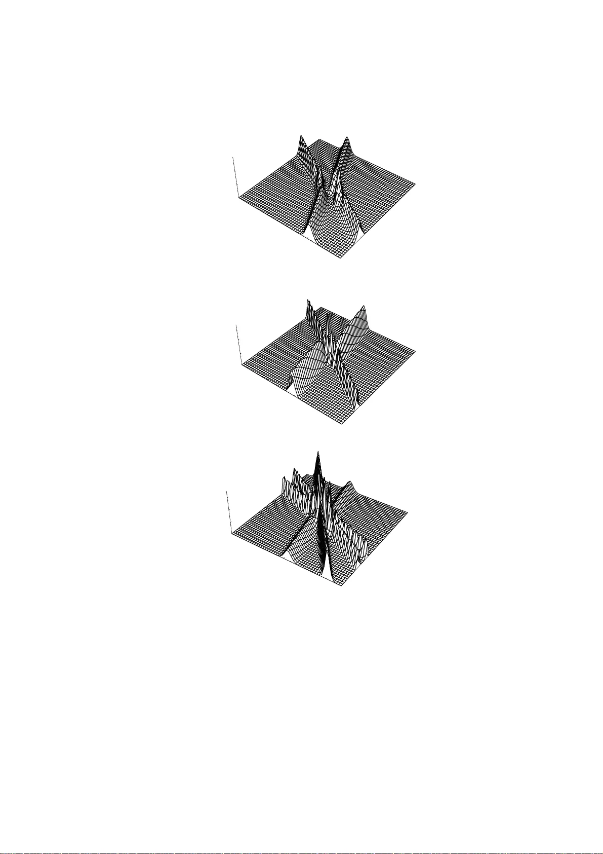
Higher dimension al brigh t solito ns and their collisio ns in m ulticomp o nen t long w a v e-s hort w a v e system T. Kanna 1 , M. Vija y a ja yan thi 2 , K. Sakk ara v arthi 1 and M. Lakshman an 2 1 Department of Physics, Bishop Heber College, Tiruchirapalli–620 017 , India 2 Cent re for Nonlinear Dynamics, Scho ol of Ph ysics, Bharathidasan University , Tiruchirapalli–620 024 , India E-mail: laksh man@cn ld.bdu.ac.in Abstract. Bright plane soliton solutions of an integrable (2 + 1) dimensional ( n + 1)- wa ve system ar e obtained by applying Hirota’s bilinearizatio n metho d. First, the soliton s olutions of a 3-wav e s y stem c onsisting of tw o shor t wav e comp onents and one long wa ve comp onent are found a nd then the re sults are generalized to the corres p o nding in tegrable ( n + 1)- wa ve system with n short wav es and single lo ng wav e. It is shown that the solitons in the short w av e comp onents (sa y S (1) and S (2) ) can be amplified by merely reducing the pulse width o f the long wa ve comp one nt (say L). The s tudy on the collisio n dynamics r eveals the int eresting b ehaviour that the solitons which split up in the short w av e comp onents undergo shap e changing collisio ns with in tensit y r edistribution and amplitude-dep endent phase shifts. Even though similar type of collisio n is possible in (1 +1) dimensional mult icomp onent in teg rable systems, to o ur knowledge for the first time we re po rt this kind o f collisio ns in (2+1) dimensions. Howev e r , solito ns which app ear in the long wav e comp onent exhibit only elastic collision though they under go a mplitude-depe nden t phase shifts. P A CS num b er s : 02 .30.Jr, 05.45.Yv Bright solitons in multic omp onen t LSRI system 2 1. In tro duction One of the main emphasis of curren t researc h in the area of integrable systems and their applications is the study on m ulticompo nen t no nlinear systems a dmitting soliton type solutions [1–17]. In (1+1) dimensions, it has b een sho wn that the multicomponen t brigh t solitons of the integrable N-coupled nonlinear Sc hr¨ odinger (CNLS) equations undergo fascinating shape c hang ing collisions with intensit y redistribution whic h hav e no s ingle comp onen t coun terpart [4–8]. This in teresting b eha viour fo und applicatio ns in nonlinear switc hing devices [12], matter w a ve switc hes [13] and more imp ortantly in the con text of optical computing in bulk media [14, 15]. There is a natural tendency to lo ok for suc h kind of collisions in higher dimensions. F rom this p oint of view, w e ha v e considered the follo wing recen tly studied in tegrable coupled (2+1) dimensional ((2+1 ) D) system, whic h is a tw o comp onent analogue of the t w o dimensional long w a v e- short wa v e resonance in teraction (LSRI) system [16], in dimensionless fo r m, i ( S ( j ) t + S ( j ) y ) − S ( j ) xx + LS ( j ) = 0 , j = 1 , 2 , (1 a ) L t = 2 2 X j =1 | S ( j ) | 2 x , (1 b ) where the subscripts denote partial deriv ativ es. (Note that in the ab o v e tw o comp onen ts mean tw o short w a v e ( S ) comp onen ts). The one comp onen t ( j = 1) ve rsion of the a b o v e equations corresponds to the in teraction of a long interfacial w a v e (L) and a short surface w av e (S) in a t w o la y er fluid [1 8 ]. Also in ref. [19], the existence of dromion lik e solution w a s established for the j = 1 case. In their v ery recen t in teresting w or k, O hta, Maruno and Oik aw a [16] ha v e deriv ed equation (1) as the gov erning equations for the in teraction of three nonlinear disp ersiv e w a v es b y applying a reductiv e p erturbation metho d. Here, among these t hree wa v es, t w o wa v es are propagating in the ano malous dispersion region and the third wa v e is propagat ing in the normal disp ersion r egime. In the con text of long w a ve-short w a v e in teraction, the first tw o comp o nents can b e view ed as the t w o comp onen ts of the short surface w av es while the last compo nen t corresp onds to the long interfacial wa v e. Note that the presence of the long interfacial w av e induces the nonlinear in teraction b et w een the t w o short wa v e comp o nen ts whic h leads to non trivial collision b eha viour as will b e shown in this pap er. Here on w a r ds w e call equation (1 ) as the 3 - w a ve LSRI system in whic h the first tw o comp onen ts cor r esp o nd to short w a v es and the last o ne is a long w a ve. Apart from deriving the gov erning equation (1) in ref. [16], Oh ta et al ha v e also giv en W r onskian t ype soliton solutions of a sp ecific type where the comp onen ts S (1) , S (2) , and L comprise of N solitons, M solitons, and ( M + N ) solito ns, resp ectiv ely . In this con text, how ev er, it is of considerable in terest to study the collision b eha viour if the same n um b er of solitons a re split up in all t he thr ee comp onen ts and to c hec k whether non trivial shap e c hanging collisions of solitons as in the case o f CNLS systems [4, 5] o ccur here also and to lo ok for the p ossibilities of construction of logic ga tes based on soliton collisions. F or the one comp onen t case the in teraction of t w o solito ns in b oth Bright so litons in m ultic omp onent LSRI system 3 short wa v e and long w av e comp onen ts ha v e b een studied in detail in ref. [18] and certain in teresting f eatures suc h as f usion and fission pro cesses hav e b een rev ealed. In this study , w e consider the multicomponent (2+1 ) D LSRI system admitting the same n um b er of brigh t solitons in a ll the t hree comp onen ts a nd obtain the multis oliton solutions. Our analysis on t heir collision pro p erties sho ws that t he solitons app earing in the short w av e comp onen ts exhibit a shap e c hanging collision scenario r esulting in a redistribution of in tensit y as we ll as amplitude-dep enden t phase shift whereas the long w a v e comp onent solitons undergo standar d elastic collisions only but with amplitude-dep enden t phase shifts. W e also p oint out t hat the ( N , M , N + M ) soliton solutions obta ined in ref. [16 ] follo w as sp ecial cases of the ( m, m, m ) multis oliton solution obtained here when some of the soliton par a meters are r estricted to v ery sp ecial v alues. The study is also extended to t he ( n + 1) w a v e system as w ell, where n is arbitrary . The plan of the pap er is as follo ws: In section 2, w e briefly presen t the bilinearization pro cedure fo r the three w a v e system. Multisoliton solution of the three w a ve system is discussed in section 3. Explicit one-soliton and tw o-soliton solutions are analysed in section 4. The asymptotic analysis of the t w o- soliton solution of the three w av e system is giv en in section 5. The in teresting collision scenario o f tw o solitons is discusse d in detail in section 6. Sections 7 and 8 deal with three- a nd four-solito n solutions, resp ectiv ely . Multicomp onen t case with j > 2 in equation (1) is studied in section 9. Section 10 is allotted for conclusion. 2. (2+1)D brigh t soliton solutions The soliton solutions of equation (1) are o btained by using Hirota’s direct metho d [20, 21]. By p erforming the bilinearizing transformations S ( j ) = g ( j ) f , L = − 2 ∂ 2 ∂ x 2 (log f ) , j = 1 , 2 , (2) where g ( j ) ’s are complex functions while f is a real function, equation (1) can b e decoupled in to the follow ing bilinear equations  i ( D t + D y ) − D 2 x  ( g ( j ) · f ) = 0 , j = 1 , 2 , (3 a ) D t D x ( f · f ) = − 2 2 X j =1 ( g ( j ) g ( j ) ∗ ) , (3 b ) where ∗ denotes the complex conjugat e. The Hirota’s bilinear op erator s D x , D y and D t are defined as D p x D q y D r t ( a · b ) =  ∂ ∂ x − ∂ ∂ x ′  p  ∂ ∂ y − ∂ ∂ y ′  q  ∂ ∂ t − ∂ ∂ t ′  r a ( x, y , t ) b ( x ′ , y ′ , t ′ )    ( x = x ′ ,y = y ′ ,t = t ′ ) . Expanding g ( j ) ’s and f formally as p o w er series expansions in terms of a small arbitrary real parameter χ , g ( j ) = χg ( j ) 1 + χ 3 g ( j ) 3 + . . . , j = 1 , 2 , (4 a ) f = 1 + χ 2 f 2 + χ 4 f 4 + . . . , (4 b ) Bright so litons in m ultic omp onent LSRI system 4 and solving the resultan t set of linear partial differen tial equations recursiv ely , one can obtain the explicit forms of g ( j ) and f . Then by substituting their expressions in (2) one can write dow n the soliton solutions. The pro cedure has b een successfully used to unearth sev eral inte resting prop erties of soliton collisions a sso ciated with CNLS system in Refs. [4–8]. W e hav e used a similar pro cedure here and o btained t he o ne- solito n (1, 1, 1), tw o-soliton (2, 2 , 2), three-soliton (3, 3, 3) and f o ur-soliton (4, 4, 4) solutio ns explicitly . This can b e generalized to t he arbitr ary m -soliton ( m, m, m ) solution, in a Gram determinan t form. F rom this one ma y claim that in the general case t he n um b er of solitons whic h split up in the short w a v e comp o nen ts ( S (1) and S (2) ) a s w ell a s in the long wa v e comp onen t (L) are the same. How ev er, we also p oint out that the (1, 1, 2), (2, 2, 4 ) and ( N , M , N + M ) solito n solutions o bt a ined by Ohta et al [16] can b e deduced as sp ecial cases of o ur ( m, m, m ) solito n solution with m = 2 , m = 4 and m = N + M , resp ectiv ely , f o r par ticular c hoices of parameters in the solutions. 3. Arbitrary m-soliton solution W e first presen t the general form of ( m, m, m ) soliton solution for arbitrary m in t he follo wing Gra m determinan t form. In order to write down the m ultisoliton ( m -soliton) solution of the three w av e LSRI system (1 ), w e define the follo wing (1 × m ) row matrix C s , s = 1 , 2 , ( m × 1) column matrices ψ j , and φ , j = 1 , 2 , . . . , m , and the ( m × m ) iden tity matrix I : C s = −  α ( s ) 1 , α ( s ) 2 , . . . , α ( s ) m  , 0 = (0 , 0 , . . . , 0) , (5 a ) ψ j = α (1) j α (2) j ! , φ =      e η 1 e η 2 . . . e η m      , I =      1 0 · · · 0 0 1 · · · 0 . . . . . . . . . . . . 0 0 · · · 1      . (5 b ) Here α ( s ) j , s = 1 , 2, j = 1 , 2 , . . . , m , are ar bitr ary complex pa rameters and η i = k i x − ( ik 2 i + ω i ) y + ω i t , i = 1 , 2 , . . . , m , and k i and ω i are complex parameters. Then w e can write dow n the m ultisoliton solution of the three w av e LSRI system in the form of equation (2), with S ( s ) = g ( s ) f , s = 1 , 2 , L = − 2 ∂ 2 ∂ x 2 log( f ) , (6) where g ( s ) =        A I φ − I B 0 T 0 C s 0        , f =      A I − I B      , (7 a ) in whic h s denotes the short w av e comp onen ts. Here the matrices A and B are defined as A ij = e η i + η j k i + k ∗ j , B ij = κ j i = − ψ † i ψ j ( ω ∗ i + ω j ) = − ( α (1) j α (1) ∗ i + α (2) j α (2) ∗ i ) ( ω ∗ i + ω j ) , i, j = 1 , 2 , . . . , m. (7 b ) Bright so litons in m ultic omp onent LSRI system 5 In equation (7 b ), † represen ts the transp ose conjugate and the real parts o f ω i ’s (or k i ’s) should b e c hosen as negativ e quantities in order to obtain nonsingular solutions, whic h are necessary conditions. Sufficiency condition requires the choice of parameters suc h that f is real and nonzero (see b elo w sections 4, 7 and 8 for details in the case of m = 1 , 2 , 3 , and 4). 3.1. Pr o of of multisoliton solution of the thr e e wa ve LSRI system W e no w prov e that the Gra m determinant forms of g ( s ) and f giv en ab o v e indeed satisfy the bilinear equations (3). By applying the deriv ative form ula for the determinan ts, tha t is, ∂ D ∂ x = X 1 ≤ i,j ≤ n ∂ a i,j ∂ x ∂ D ∂ a i,j = X 1 ≤ i,j ≤ n ∂ a i,j ∂ x ∆ i,j , (8 a ) where D =          a 11 a 12 · · · a 1 n a 21 a 22 · · · a 2 n . . . . . . . . . . . . a n 1 a n 2 · · · a nn          and ∆ i,j is the cofactor of the ( i, j ) th elemen t and making use of the prop erties of b ordered determinan ts and also the elemen tary prop erties of determinan ts [21, 22], the deriv ativ es g ( s ) x , f x , f t , f xt , g ( s ) z , g ( s ) xx , f z and f xx , where ∂ ∂ z =  ∂ ∂ t + ∂ ∂ y  , can b e deriv ed as b elo w: g ( s ) x =          A I φ φ x − I B 0 T 0 T 0 C s 0 0 0 0 − 1 0          , f x =        A I φ − I B 0 T − φ † 0 0        , (8 b ) f t = − 2 X s =1        A I 0 T − I B − C † s 0 C s 0        , f xt = − 2 X s =1          A I φ 0 T − I B 0 T − C † s − φ † 0 0 0 0 C s 0 0          , (8 c ) g ( s ) z = − i          A I φ φ xx − I B 0 T 0 T 0 C s 0 0 0 0 − 1 0          + i          A I φ φ x − I B 0 T 0 T 0 C s 0 0 φ † 0 0 0          , (8 d ) g ( s ) xx =          A I φ φ xx − I B 0 T 0 T 0 C s 0 0 0 0 − 1 0          +          A I φ φ x − I B 0 T 0 T 0 C s 0 0 φ † 0 0 0          , (8 e ) Bright so litons in m ultic omp onent LSRI system 6 f z = − i        A I φ x − I B 0 T − φ † 0 0        + i        A I φ − I B 0 T − φ † x 0 0        , (8 f ) and f xx =        A I φ x − I B 0 T − φ † 0 0        +        A I φ − I B 0 T − φ † x 0 0        . (8 g ) The conjugate of g ( s ) can b e written as g ( s ) ∗ = −        A I 0 T − I B − C † s − φ † 0 0        . (8 h ) Substituting for g ( s ) x , g ( s ) z , g ( s ) xx , f x , f xx , and f z in equation (3a) , we find          A I φ φ x − I B 0 T 0 T 0 C s 0 0 − φ † 0 0 0               A I − I B      =        A I φ x − I B 0 T − φ † 0 0               A I φ − I B 0 T 0 C s 0        −        A I φ x − I B 0 T 0 C s 0               A I φ − I B 0 T − φ † 0 0        . (8 i ) This is nothing but a Jacobian iden tit y and hence g ( s ) and f satisfy the fir st bilinear equation (3a). In a similar w a y one can also c heck that the second bilinear equation (3b) giv es rise t o the follow ing Jacobian iden tit y fo r the Gram determinan t f o rms of g ( s ) and f : − 2 X s =1          A I φ 0 T − I B 0 T − C † s − φ † 0 0 0 0 C s 0 0               A I − I B      = − 2 X s =1        A I 0 T − I B − C † s 0 C s 0               A I φ − I B 0 T − φ † 0 0        + 2 X s =1        A I φ − I B 0 T 0 C s 0               A I 0 T − I B − C † s − φ † 0 0        . (8 j ) Th us equations (8i) and (8 j) clearly show that t he giv en Gram determinants g ( s ) and f satisfy the bilinear equations (3) , whic h completes the pro of o f (6) with (7). 3.2. ( N , M , N + M ) soliton s olution W e now p o in t out that the ( N , M , N + M ) soliton solution (for N ev en) giv en in ref. [16] can b e obtained a s a sp ecial case of the ab ov e ( m, m, m ) soliton solution for the sp ecific Bright so litons in m ultic omp onent LSRI system 7 c ho ice of parameters α (2) i = 0 , i = 1 , 2 , . . . , N , and α (1) l = 0 , l = N + 1 , N + 2 , . . . , m (= N + M ) alo ng with the para metric restrictions α (1) i = Q m j =1 ( k i + k ∗ j ) Q m j =1 ,i 6 = j ( k j − k i ) , i = 1 , 2 , . . . , N , α (2) l = Q m j =1 ( k l + k ∗ j ) Q m j =1 ,l 6 = j ( k j − k l ) , l = N + 1 , N + 2 , . . . , m (= N + M ) . In the following sections, w e will consider t he explicit cases of m = 1 , 2 , 3, a nd 4 soliton solutions and the nature of the soliton inte ractions therein. 4. One-soliton (1, 1, 1) and tw o-soliton (2, 2, 2) solutions Sp ecializing to the case of m = 1 in equation (6) so that t he Gram determinants tak e the form g ( j ) =        A 11 1 e η 1 − 1 B 11 0 0 − α ( j ) 1 0        , f =      A 11 1 − 1 B 11      , j = 1 , 2 , (9) where A 11 = e η 1 + η ∗ 1 k 1 + k ∗ 1 , and B 11 = κ 11 = − ( | α (1) 1 | 2 + | α (2) 1 | 2 ) ω 1 + ω ∗ 1 . One can write down the explicit one-soliton solution as S ( j ) = α ( j ) 1 e η 1 1 + e η 1 + η ∗ 1 + R , j = 1 , 2 , (10 a ) L = − 2 ∂ 2 ∂ x 2  log  1 + e η 1 + η ∗ 1 + R  , (10 b ) where η 1 = k 1 x − ( ik 2 1 + ω 1 ) y + ω 1 t, e R = − P 2 j =1 ( α ( j ) 1 α ( j ) ∗ 1 ) 4 k 1 R ω 1 R , (10 c ) k 1 = k 1 R + ik 1 I , ω 1 = ω 1 R + iω 1 I . (10 d ) Here α (1) 1 , α (2) 1 , ω 1 and k 1 are all complex parameters. In equation (10 ) the suffixes R and I denote t he real and imaginary parts, resp ectiv ely . It ma y b e noted that this brigh t soliton solution is nonsingular only when k 1 R ω 1 R < 0, otherwise equation (10) b ecomes singular. In this work, the main fo cus will b e on nonsingular solutions as they are of ph ysical imp ortance. The ab ov e one-soliton solution can a lso b e rewritten as S ( j ) = A j p k 1 R ω 1 R e iη 1 I sec h  η 1 R + R 2  , j = 1 , 2 , (11 a ) L = − 2 k 2 1 R sec h 2  η 1 R + R 2  , (11 b ) where η 1 R = k 1 R x + (2 k 1 R k 1 I − ω 1 R ) y + ω 1 R t and A j = α ( j ) 1  | α (1) 1 | 2 + | α (2) 1 | 2  1 2 , j = 1 , 2 . Bright so litons in m ultic omp onent LSRI system 8 The complex quan t it ies A j √ k 1 R ω 1 R , j = 1 , 2 , represen t the amplitude of t he soliton in the S ( j ) comp onen ts whereas th y real quan tit y 2 k 2 1 R giv es t he amplitude of t he soliton in the comp onen t − L . Note that the complex quantities A 1 and A 2 satisfy t he relation | A 1 | 2 + | A 2 | 2 = 1, whic h is a reflection of the fact that the set of equation ( 1 ) is rotationally symmetric in the ( S (1) , S (2) ) space. F or illustrativ e purp ose, let us obtain the soliton solution f or the sp ecial c hoice of parameters ω 1 = − ik 2 1 / 2. In t his case, the ab ov e soliton solution (11) b ecomes S ( j ) = A j k 1 R p k 1 I e iη 1 I sec h  η 1 R + R 2  , j = 1 , 2 , (12 a ) L = − 2 k 2 1 R sec h 2  η 1 R + R 2  , (12 b ) where η 1 = k 1 x − ik 2 1 2 ( t + y ) , e R = P 2 j =1 ( α ( j ) 1 α ( j ) ∗ 1 ) − 4 k 2 1 R k 1 I , k 1 = k 1 R + ik 1 I , ( 12 c ) The ab ov e soliton solution is nonsingular only when k 1 I ≤ 0, otherwise the parameter R in equation (12 c ) b ecomes complex and the solution (12) b ecomes singular. Inte restingly , w e observ e that by just reducing the width of the soliton in t he L comp onent (which is prop or t ional to k 1 I ) without affecting its amplitude, the soliton in the S (1) and S (2) comp onen ts can b e amplified with a prop o r t ionate pulse compression, a desirable prop ert y for a pulse in nonlinear optics. 4.1. Two-soliton (2, 2, 2) solution T o obtain the tw o solito n solution, w e take m = 2 in equation (7) and deduce the G r a m determinan t forms as g ( j ) =            A 11 A 12 1 0 e η 1 A 21 A 22 0 1 e η 2 − 1 0 B 11 B 12 0 0 − 1 B 21 B 22 0 0 0 − α ( j ) 1 − α ( j ) 2 0            , f =          A 11 A 12 1 0 A 21 A 22 0 1 − 1 0 B 11 B 12 0 − 1 B 21 B 22          , ( 1 3) where A ij = e η i + η ∗ j k i + k ∗ j , and B ij = κ j i = −  α (1) j α (1) ∗ i + α (2) j α (2) ∗ i  ( ω j + ω ∗ i ) , i, j = 1 , 2. W e can then write the explicit form of the (2, 2, 2) soliton solution as S ( j ) = 1 f  α ( j ) 1 e η 1 + α ( j ) 2 e η 2 + e η 1 + η ∗ 1 + η 2 + δ 1 j + e η 2 + η ∗ 2 + η 1 + δ 2 j  , j = 1 , 2 , (14 a ) L = − 2 ∂ 2 ∂ x 2 log( f ) , (14 b ) where f = 1 + e η 1 + η ∗ 1 + R 1 + e η 1 + η ∗ 2 + δ 0 + e η 2 + η ∗ 1 + δ ∗ 0 + e η 2 + η ∗ 2 + R 2 + e η 1 + η ∗ 1 + η 2 + η ∗ 2 + R 3 . (14 c ) Bright so litons in m ultic omp onent LSRI system 9 The v ar io us quan tit ies found in equation (14) are defined as b elow: η i = k i x − ( ik 2 i + ω i ) y + ω i t, i = 1 , 2 , e R 1 = κ 11 ( k 1 + k ∗ 1 ) , (15 a ) e R 2 = κ 22 ( k 2 + k ∗ 2 ) , e δ 0 = κ 12 ( k 1 + k ∗ 2 ) , e δ ∗ 0 = κ 21 ( k 2 + k ∗ 1 ) , (15 b ) e δ 1 j = ( k 1 − k 2 ) ( k 1 + k ∗ 1 )( k 2 + k ∗ 1 ) ( α ( j ) 1 κ 21 − α ( j ) 2 κ 11 ) , (15 c ) e δ 2 j = ( k 2 − k 1 ) ( k 2 + k ∗ 2 )( k 1 + k ∗ 2 ) ( α ( j ) 2 κ 12 − α ( j ) 1 κ 22 ) , j = 1 , 2 , (15 d ) e R 3 = | k 1 − k 2 | 2 ( k 1 + k ∗ 1 )( k 2 + k ∗ 2 ) | k 1 + k ∗ 2 | 2 ( κ 11 κ 22 − κ 12 κ 21 ) , (15 e ) κ il = −  α (1) i α (1) ∗ l + α (2) i α (2) ∗ l  ( ω i + ω ∗ l ) , i, l = 1 , 2 . The t w o- soliton solution is c haracterized by eigh t arbitr ary complex parameters α (1) 1 , α (2) 1 , α (1) 2 , α (2) 2 , k 1 , k 2 , ω 1 and ω 2 . The ab ov e solution feat ur es b oth singular and nonsingular solutions. The nonsingular solution can b e obtained b y requiring the denominator f in (14) t o b e real a nd nonzero. The expression (1 4 c) for f can b e rewritten as f = 2 e η 1 R + η 2 R  e ( R 1 + R 2 ) / 2 cosh ( η 1 R − η 2 R + ( R 1 + R 2 ) / 2) + e δ 0 R cos ( η 1 I − η 2 I + δ 0 I ) + e R 3 / 2 cosh ( η 1 R + η 2 R + R 3 / 2)  . (15 f ) T o get regular solutions, e R 1 and e R 2 should b e p ositiv e whic h can b e obtained only for k 1 R ω 1 R < 0 a nd k 2 R ω 2 R < 0, resp ectiv ely . Otherwise, that is fo r negativ e v alues, the solution is not regular as in this case R 1 and R 2 app earing in t he argumen t of cosh in first term b ecome complex. So the condition k j R ω j R < 0 , j = 1 , 2 is a necessary condition to obta in regular solution. In a similar w a y , in the third term, the quan tit y R 3 / 2 b ecomes real and p o sitiv e f or the conditio n κ 11 κ 22 − | κ 12 | 2 > 0, as may b e seen from equation (15e). Still the middle term cos( η 1 I − η 2 I + δ 0 I ) can lead to a singularit y as it oscillates b et w een -1 a nd 1. This can b e eliminated b y c ho osing the co efficien t s of the remaining t w o terms as e ( R 1 + R 2 ) / 2 + e R 3 / 2 > e δ 0 R , in o rder to ensure that f will not b e zero at an y p oin t in space and time. The last condition is a sufficien t one. As an illustration, the in teraction of tw o solitons in system (1) is sho wn in fig ur e 1. The parameters a r e c ho sen as k 1 = 1 − 2 i , k 2 = 1 . 5 − 1 . 05 i , ω 1 = − 1 − i , ω 2 = − 1 . 3 − 0 . 5 i , α (1) 1 = 2, α (1) 2 = α (2) 1 = 1, α (2) 2 = 0 . 01 . One observ es that the solitons in the S (1) and S (2) comp onen ts undergo shap e c hanging (energy redistribution) collisions while there is only elastic collision in the L comp onent. More details are giv en in section 6 b elo w. 4.2. (1, 1, 2) soliton solution of Ohta et al No w we show that the (1, 1, 2 ) soliton solution obtained b y Oh ta et al [16] is a sp ecial case of the a b ov e t w o-soliton (2, 2, 2) solution (14). Sp ecifically , for the sp ecial c hoice Bright so litons in m ultic omp onent LSRI system 10 of the parameters α (1) 2 = α (2) 1 = 0 , the ab o v e t w o-soliton solution b ecomes S (1) = 1 f  α (1) 1 e η 1 + e η 2 + η ∗ 2 + η 1 + δ 21  , (16 a ) S (2) = 1 f  α (2) 2 e η 2 + e η 1 + η ∗ 1 + η 2 + δ 12  , (16 b ) L = − 2 ∂ 2 ∂ x 2 (log( f )) , (16 c ) where f = 1 + e η 1 + η ∗ 1 + R 1 + e η 2 + η ∗ 2 + R 2 + e η 1 + η ∗ 1 + η 2 + η ∗ 2 + R 3 . (16 d ) The v ar io us other parameters defined in equations (14) now tak e the forms e R 1 = κ 11 ( k 1 + k ∗ 1 ) , e R 2 = κ 22 ( k 2 + k ∗ 2 ) , e δ 0 = e δ 11 = e δ 22 = 0 , (16 e ) e δ 12 = − α (2) 2 κ 11 ( k 1 − k 2 ) ( k 1 + k ∗ 1 )( k 2 + k ∗ 1 ) , e δ 21 = − α (1) 1 κ 22 ( k 2 − k 1 ) ( k 2 + k ∗ 2 )( k 1 + k ∗ 2 ) , (16 f ) e R 3 = | k 1 − k 2 | 2 κ 11 κ 22 ( k 1 + k ∗ 1 )( k 2 + k ∗ 2 ) | k 1 + k ∗ 2 | 2 , ( 1 6 g ) κ 11 = − | α (1) 1 | 2 ( ω 1 + ω ∗ 1 ) , κ 22 = − | α (2) 2 | 2 ( ω 2 + ω ∗ 2 ) . (16 h ) Solution ( 16a-h) is not hing but the (1, 1, 2) soliton solution obtained b y O hta et al in ref. [16] when the parameters in (16a- h) are further restricted to the sp ecial c hoice α (1) 1 = ( k 1 + k ∗ 1 )( k 1 + k ∗ 2 ) ( k 2 − k 1 ) and α (2) 2 = ( k 2 + k ∗ 2 )( k 2 + k ∗ 1 ) ( k 2 − k 1 ) . (16 i ) 5. Asymptotic analysis of t he tw o soliton solution (14) of t he three wa v e system W e now consider the collision prop erties a sso ciated with the general tw o-soliton solution (14) of the t hree w a v e system. F or this purp ose w e carry out the analysis, fo r k j R > 0, ω j R < 0 , j = 1 , 2. Als o w e c ho ose k 2 R k 1 R >    ω 2 R ω 1 R    and k 2 R k 2 I k 1 R k 1 I >    ω 2 R ω 1 R    for con v enience. Similar analysis can b e p erformed for other c hoices of k j R ’s and ω j R ’s also b y keep ing k j R > 0, ω j R < 0, whic h is the necessary condition for nonsingular solutions. W e no w define the soliton w a v e v ariables as η 1 R = k 1 R x + (2 k 1 R k 1 I − ω 1 R ) y + ω 1 R t and η 2 R = k 2 R x + (2 k 2 R k 2 I − ω 2 R ) y + ω 2 R t . In the limit x, y → ±∞ and a fixed t the t w o- soliton solution (14) take s the following asymptotic forms. a) Before collision (limit x, y → −∞ ): (i) So lit o n 1 ( η 1 R ≃ 0 , η 2 R → −∞ ):    S (1) S (2)    ≃    A 1 − 1 A 1 − 2    p k 1 R ω 1 R sec h  η 1 R + R 1 2  e iη 1 I , (17 a ) L ≃ − 2 k 2 1 R sec h 2  η 1 R + R 1 2  , (17 b ) Bright so litons in m ultic omp onent LSRI system 11 where    A 1 − 1 A 1 − 2    ≃    α (1) 1 α (2) 1    e − R 1 / 2 (( k 1 + k ∗ 1 )( ω 1 + ω ∗ 1 )) 1 / 2 . (17 c ) (ii) So lit o n 2 ( η 2 R ≃ 0 , η 1 R → ∞ ):    S (1) S (2)    ≃    A 2 − 1 A 2 − 2    p k 2 R ω 2 R sec h  η 2 R + ( R 3 − R 1 ) 2  e iη 2 I , (1 8 a ) L ≃ − 2 k 2 2 R sec h 2  η 2 R + ( R 3 − R 1 ) 2  , (18 b ) where    A 2 − 1 A 2 − 2    ≃    e δ 11 e δ 12    e − ( R 1 + R 3 ) / 2 (( k 2 + k ∗ 2 )( ω 2 + ω ∗ 2 )) 1 / 2 . (18 c ) The v arious quan tit ies in the ab o v e expressions a r e defined in equation (15). b) After collision (limit x, y → ∞ ): (i) So lit o n 1 ( η 1 R ≃ 0 , η 2 R → ∞ ):    S (1) S (2)    ≃    A 1+ 1 A 1+ 2    p k 1 R ω 1 R sec h  η 1 R + ( R 3 − R 2 ) 2  e iη 1 I , (1 9 a ) L ≃ − 2 k 2 1 R sec h 2  η 1 R + ( R 3 − R 2 ) 2  , (19 b ) where    A 1+ 1 A 1+ 2    ≃    e δ 21 e δ 22    e − ( R 2 + R 3 ) / 2 (( k 1 + k ∗ 1 )( ω 1 + ω ∗ 1 )) 1 / 2 . (19 c ) (ii) So lit o n 2 ( η 2 R ≃ 0 , η 1 R → −∞ ):    S (1) S (2)    ≃    A 2+ 1 A 2+ 2    p k 2 R ω 2 R sec h  η 2 R + R 2 2  e iη 2 I , (20 a ) L ≃ − 2 k 2 2 R sec h 2  η 2 R + R 2 2  , (20 b ) where    A 2+ 1 A 2+ 2    ≃    α (1) 2 α (2) 2    e − R 2 / 2 (( k 2 + k ∗ 2 )( ω 2 + ω ∗ 2 )) 1 / 2 . (20 c ) Bright so litons in m ultic omp onent LSRI system 12 Note that in all the ab o v e expressions   A j ± 1   2 +   A j ± 2   2 = 1, j = 1 , 2. Our ab ov e analysis rev eals the fact that due to collision the amplitude of t he colliding solitons, sa y s 1 and s 2 in the S (1) and S (2) comp onen ts, c hang e from  A 1 − 1 , A 1 − 2  √ k 1 R ω 1 R and  A 2 − 1 , A 2 − 2  √ k 2 R ω 2 R to  A 1+ 1 , A 1+ 2  √ k 1 R ω 1 R and  A 2+ 1 , A 2+ 2  √ k 2 R ω 2 R , resp ectiv ely . Here the sup erscripts in A j ± i ’s with i, j = 1 , 2 denote the solito ns s 1 and s 2 , while the subscripts represen t the comp onents S (1) and S (2) and the “ ± ” signs stand for “ x, y → ±∞ ”. In addition to this c hange in the amplitudes, the solitons also undergo amplitude-dep enden t phase shifts due to the collision and they can b e determined straigh tforw ardly from the ab o v e asymptotic express ions. F rom equations ((17) a nd (19)) and equations ((18) a nd (20)), one can easily c hec k that the phase shift suffered b y t he soliton s 1 (sa y Φ 1 ) = − Phase shift of soliton s 2 (sa y − Φ 2 ≡ Φ 1 ) = Φ and is giv en b y Φ = ( R 3 − R 1 − R 2 ) 2 , (21) where R 1 , R 2 and R 3 are as defined in equation (15) and dep ends on t he a mplitudes. 6. Soliton Interaction No w it is of further in terest to analyze the in teraction prop erties of the solitons depicted in figure 1 for the sp ecific set of v alues of the parameters giv en in section 4 .1. Figure 1 sho ws typical spatial collision of tw o solitons fo r t = − 4 corresp onding to the exact expression (14 ). The in teresting collision scenario depicted in figure 1 clearly indicates that there is a redistribution of intens it y among the t w o S ( j ) comp onen ts resulting in an enhancemen t (suppression) of in tensit y of solitons s 2 ( s 1 ) in the S (1) comp onen t and a suppression (enhancemen t) of soliton s 2 ( s 1 ) in the S (2) comp onen t. The solitons also undergo amplitude-dep enden t phase shifts along with this energy redistribution. Ho w ev er, the solitons app earing in the long wa v e comp onen t ( L ) exhibit the standard elastic collision a s sho wn in the third figure of figure 1 though the phase shift here is also amplitude-dep enden t. In terestingly , if t he parameters are so c ho sen suc h tha t the condition α (1) 1 α (1) 2 = α (2) 1 α (2) 2 is satisfied, there o ccurs only elastic collision in all the thr ee comp onen ts S ( j ) and L . The underlying collision dynamics can b e w ell understo o d b y using the asymptotic analysis of the t w o - soliton solution ( 1 4) discussed in section 5 and is further describ ed b elow . 6.1. Col lision b ehavi our of solitons in the short wave c om p onents The asymptotic analysis presen ted in the previous section also results in the following expressions relating the intensities of solitons s 1 and s 2 in the S (1) and S (2) comp onen ts b efore and after inte raction, | A j + i | 2 = | T i j | 2 | A j − i | 2 , i, j = 1 , 2 , (22 a ) where the sup erscripts j ± represen t the solitons designated a s s 1 and s 2 at “ x, y → ±∞ ”. The expression for the transition in tensities for the solitons in t he short w a v e comp onen ts Bright so litons in m ultic omp onent LSRI system 13 can b e written do wn using the results in equations (17 c ), (1 8 c ), ( 1 9 c ) and (20 c ) a s | T 1 j | 2 = | 1 − λ 2 ( α ( j ) 2 /α ( j ) 1 ) | 2 | 1 − λ 1 λ 2 | , (22 b ) | T 2 j | 2 = | 1 − λ 1 λ 2 | | 1 − λ 1 ( α ( j ) 1 /α ( j ) 2 ) | 2 , j = 1 , 2 , (22 c ) λ 1 = κ 21 κ 11 , λ 2 = κ 12 κ 22 . (22 d ) In general   T i j   6 = 1 and so an in tensit y (energy) redistribution of the solito ns in the S (1) and S (2) comp onen ts o ccurs as sho wn in figure 1. One can notice that the standar d elastic collision tak es place for the sp ecific pa rametric choice α (1) 1 α (1) 2 = α (2) 1 α (2) 2 , as | T i j | 2 = 1 and hence | A j − i | 2 = | A j + i | 2 , i, j = 1 , 2 , for this choice . Ho w ev er t he t w o colliding solitons s 1 and s 2 suffer amplitude-dep enden t phase shifts Φ 1 and Φ 2 , resp ectiv ely , a s given in equation (21). 6.2. Col lision sc enario in the long wave c omp onent In the L comp onen t, there o ccurs only elastic collision for an y pa r a metric c hoice. This is eviden t from the asymptotic analysis, vide equations (17b), (18b), (1 9 b) and (20b). One finds t ha t the amplitudes of the solitons s 1 and s 2 b efore and after in teraction are the same whic h are − 2 k 2 1 R and − 2 k 2 2 R , resp ectiv ely , while there o ccurs an amplitude- dep enden t phase shift as given by equation (21). 6.3. Shap e changing c ol l isions and Line ar fr actional tr ansf ormations It is instructiv e to notice that the intens it y redistribution in the short w a v e comp onen ts c ha racterized b y the transition matrices (equation (22 )) can also b e view ed as a linear fractional tr ansformation (LF T). T o r ealize this, we re- express the amplitude changes in the short w a v e comp onen ts of soliton s 1 after in t era ctio n as A 1+ 1 = Γ C 11 A 1 − 1 + Γ C 12 A 1 − 2 , (23 a ) A 1+ 2 = Γ C 21 A 1 − 1 + Γ C 22 A 1 − 2 . (23 b ) Here Γ =  a a ∗  c h ( α (1) 1 α (1) ∗ 2 + α (2) 1 α (2) ∗ 2 )( α (1) 2 α (1) ∗ 2 + α (2) 2 α (2) ∗ 2 ) i − 1 , (23 c ) C 11 = − h ( α (1) 2 α (1) ∗ 2 )( ω 1 − ω 2 ) + ( α (2) 2 α (2) ∗ 2 )( ω 1 + ω ∗ 2 ) i , (23 d ) C 12 = ( α (1) 2 α (2) ∗ 2 )( ω 2 + ω ∗ 2 ) , (23 e ) C 21 = ( α (2) 2 α (1) ∗ 2 )( ω 2 + ω ∗ 2 ) , (23 f ) C 22 = − h ( α (1) 2 α (1) ∗ 2 )( ω 1 + ω ∗ 2 ) + ( α (2) 2 α (2) ∗ 2 )( ω 1 − ω 2 ) i , (23 g ) where c =  1 | κ 12 | 2 − 1 κ 11 κ 22  − 1 / 2 , (23 h ) Bright so litons in m ultic omp onent LSRI system 14 a = h − ( k 1 − k 2 )( k 2 + k ∗ 1 )( ω 2 + ω ∗ 1 )( α (1) 1 α (1) ∗ 2 + α (2) 1 α (2) ∗ 2 ) i 1 / 2 . (23 i ) Note that t he co efficien ts C ij ’s, i, j = 1 , 2 , are indep endent of α ( j ) 1 ’s a nd so of A 1 − 1 and A 1 − 2 , that is the α parameters of soliton s 1 . F rom equations (23 a ) a nd (23 b ), ρ 1+ 1 , 2 = A 1+ 1 A 1+ 2 = C 11 ρ 1 − 1 , 2 + C 12 C 21 ρ 1 − 1 , 2 + C 22 , ( 2 3 j ) where ρ 1 − 1 , 2 = A 1 − 1 A 1 − 2 , in which the sup erscripts represen t the underlying solito n a nd the subscripts r epresen t the corr esp o nding short w a v e compo nen ts. Th us the stat e of s 1 b efore and after in teraction is c haracterized b y the complex quantities ρ 1 − 1 , 2 and ρ 1+ 1 , 2 , resp ectiv ely . The direct consequence of the ab o v e L F T represen tation is the iden tificatio n of a binar y lo gic using soliton collisions as in the case of CNLS equations [6, 14, 15] and hence the LFT can b e profitably used to construct logic gates asso ciated with the binary logic. A similar analysis can b e made for the soliton s 2 also. 7. Th ree-soliton (3, 3, 3) solution F rom the general form (7), and r estricting m = 3, one can write do wn the explicit three-soliton (3, 3, 3) solution as S ( j ) = α ( j ) 1 e η 1 + α ( j ) 2 e η 2 + α ( j ) 3 e η 3 + e η 1 + η ∗ 1 + η 2 + δ 1 j + e η 1 + η ∗ 1 + η 3 + δ 2 j + e η 2 + η ∗ 2 + η 1 + δ 3 j f + e η 2 + η ∗ 2 + η 3 + δ 4 j + e η 3 + η ∗ 3 + η 1 + δ 5 j + e η 3 + η ∗ 3 + η 2 + δ 6 j + e η ∗ 1 + η 2 + η 3 + δ 7 j + e η 1 + η ∗ 2 + η 3 + δ 8 j f + e η 1 + η 2 + η ∗ 3 + δ 9 j + e η 1 + η ∗ 1 + η 2 + η ∗ 2 + η 3 + τ 1 j + e η 1 + η ∗ 1 + η 3 + η ∗ 3 + η 2 + τ 2 j f + e η 2 + η ∗ 2 + η 3 + η ∗ 3 + η 1 + τ 3 j f , j = 1 , 2 , (24 a ) where f = 1 + e η 1 + η ∗ 1 + R 1 + e η 2 + η ∗ 2 + R 2 + e η 3 + η ∗ 3 + R 3 + e η 1 + η ∗ 2 + δ 10 + e η ∗ 1 + η 2 + δ ∗ 10 + e η 1 + η ∗ 3 + δ 20 + e η ∗ 1 + η 3 + δ ∗ 20 + e η 2 + η ∗ 3 + δ 30 + e η ∗ 2 + η 3 + δ ∗ 30 + e η 1 + η ∗ 1 + η 2 + η ∗ 2 + R 4 + e η 1 + η ∗ 1 + η 3 + η ∗ 3 + R 5 + e η 2 + η ∗ 2 + η 3 + η ∗ 3 + R 6 + e η 1 + η ∗ 1 + η 2 + η ∗ 3 + τ 10 + e η 1 + η ∗ 1 + η 3 + η ∗ 2 + τ ∗ 10 + e η 2 + η ∗ 2 + η 1 + η ∗ 3 + τ 20 + e η 2 + η ∗ 2 + η ∗ 1 + η 3 + τ ∗ 20 + e η 3 + η ∗ 3 + η 1 + η ∗ 2 + τ 30 + e η 3 + η ∗ 3 + η ∗ 1 + η 2 + τ ∗ 30 + e η 1 + η ∗ 1 + η 2 + η ∗ 2 + η 3 + η ∗ 3 + R 7 . (24 b ) Here η i = k i x − ( ik 2 i + ω i ) y + ω i t, i = 1 , 2 , 3 , (24 c ) e δ 1 j = ( k 1 − k 2 )( α ( j ) 1 κ 21 − α ( j ) 2 κ 11 ) ( k 1 + k ∗ 1 )( k ∗ 1 + k 2 ) , e δ 2 j = ( k 1 − k 3 )( α ( j ) 1 κ 31 − α ( j ) 3 κ 11 ) ( k 1 + k ∗ 1 )( k ∗ 1 + k 3 ) , e δ 3 j = ( k 1 − k 2 )( α ( j ) 1 κ 22 − α ( j ) 2 κ 12 ) ( k 1 + k ∗ 2 )( k 2 + k ∗ 2 ) , e δ 4 j = ( k 2 − k 3 )( α ( j ) 2 κ 32 − α ( j ) 3 κ 22 ) ( k 2 + k ∗ 2 )( k ∗ 2 + k 3 ) , Bright so litons in m ultic omp onent LSRI system 15 e δ 5 j = ( k 1 − k 3 )( α ( j ) 1 κ 33 − α ( j ) 3 κ 13 ) ( k 3 + k ∗ 3 )( k ∗ 3 + k 1 ) , e δ 6 j = ( k 2 − k 3 )( α ( j ) 2 κ 33 − α ( j ) 3 κ 23 ) ( k ∗ 3 + k 2 )( k ∗ 3 + k 3 ) , e δ 7 j = ( k 2 − k 3 )( α ( j ) 2 κ 31 − α ( j ) 3 κ 21 ) ( k ∗ 1 + k 2 )( k ∗ 1 + k 3 ) , e δ 8 j = ( k 1 − k 3 )( α ( j ) 1 κ 32 − α ( j ) 3 κ 12 ) ( k 1 + k ∗ 2 )( k ∗ 2 + k 3 ) , e δ 9 j = ( k 1 − k 2 )( α ( j ) 1 κ 23 − α ( j ) 2 κ 13 ) ( k 1 + k ∗ 3 )( k 2 + k ∗ 3 ) , e τ 1 j = ( k 2 − k 1 )( k 3 − k 1 )( k 3 − k 2 )( k ∗ 2 − k ∗ 1 ) ( k ∗ 1 + k 1 )( k ∗ 1 + k 2 )( k ∗ 1 + k 3 )( k ∗ 2 + k 1 )( k ∗ 2 + k 2 )( k ∗ 2 + k 3 ) × h α ( j ) 1 ( κ 21 κ 32 − κ 22 κ 31 ) + α ( j ) 2 ( κ 12 κ 31 − κ 32 κ 11 ) + α ( j ) 3 ( κ 11 κ 22 − κ 12 κ 21 ) i , e τ 2 j = ( k 2 − k 1 )( k 3 − k 1 )( k 3 − k 2 )( k ∗ 3 − k ∗ 1 ) ( k ∗ 1 + k 1 )( k ∗ 1 + k 2 )( k ∗ 1 + k 3 )( k ∗ 3 + k 1 )( k ∗ 3 + k 2 )( k ∗ 3 + k 3 ) × h α ( j ) 1 ( κ 33 κ 21 − κ 31 κ 23 ) + α ( j ) 2 ( κ 31 κ 13 − κ 11 κ 33 ) + α ( j ) 3 ( κ 23 κ 11 − κ 13 κ 21 ) i , e τ 3 j = ( k 2 − k 1 )( k 3 − k 1 )( k 3 − k 2 )( k ∗ 3 − k ∗ 2 ) ( k ∗ 2 + k 1 )( k ∗ 2 + k 2 )( k ∗ 2 + k 3 )( k ∗ 3 + k 1 )( k ∗ 3 + k 2 )( k ∗ 3 + k 3 ) × h α ( j ) 1 ( κ 22 κ 33 − κ 23 κ 32 ) + α ( j ) 2 ( κ 13 κ 32 − κ 33 κ 12 ) + α ( j ) 3 ( κ 12 κ 23 − κ 22 κ 13 ) i , (24 d ) e R m = κ mm k m + k ∗ m , m = 1 , 2 , 3 , e δ 10 = κ 12 k 1 + k ∗ 2 , e δ 20 = κ 13 k 1 + k ∗ 3 , e δ 30 = κ 23 k 2 + k ∗ 3 , e R 4 = ( k 2 − k 1 )( k ∗ 2 − k ∗ 1 ) ( k ∗ 1 + k 1 )( k ∗ 1 + k 2 )( k 1 + k ∗ 2 )( k ∗ 2 + k 2 ) [ κ 11 κ 22 − κ 12 κ 21 ] , e R 5 = ( k 3 − k 1 )( k ∗ 3 − k ∗ 1 ) ( k ∗ 1 + k 1 )( k ∗ 1 + k 3 )( k ∗ 3 + k 1 )( k ∗ 3 + k 3 ) [ κ 33 κ 11 − κ 13 κ 31 ] , e R 6 = ( k 3 − k 2 )( k ∗ 3 − k ∗ 2 ) ( k ∗ 2 + k 2 )( k ∗ 2 + k 3 )( k ∗ 3 + k 2 )( k 3 + k ∗ 3 ) [ κ 22 κ 33 − κ 23 κ 32 ] , e τ 10 = ( k 2 − k 1 )( k ∗ 3 − k ∗ 1 ) ( k ∗ 1 + k 1 )( k ∗ 1 + k 2 )( k ∗ 3 + k 1 )( k ∗ 3 + k 2 ) [ κ 11 κ 23 − κ 21 κ 13 ] , e τ 20 = ( k 1 − k 2 )( k ∗ 3 − k ∗ 2 ) ( k ∗ 2 + k 1 )( k ∗ 2 + k 2 )( k ∗ 3 + k 1 )( k ∗ 3 + k 2 ) [ κ 22 κ 13 − κ 12 κ 23 ] , e τ 30 = ( k 3 − k 1 )( k ∗ 3 − k ∗ 2 ) ( k ∗ 2 + k 1 )( k ∗ 2 + k 3 )( k ∗ 3 + k 1 )( k ∗ 3 + k 3 ) [ κ 33 κ 12 − κ 13 κ 32 ] , e R 7 = | k 1 − k 2 | 2 | k 2 − k 3 | 2 | k 3 − k 1 | 2 ( k 1 + k ∗ 1 )( k 2 + k ∗ 2 )( k 3 + k ∗ 3 ) | k 1 + k ∗ 2 | 2 | k 2 + k ∗ 3 | 2 | k 3 + k ∗ 1 | 2 × [( κ 11 κ 22 κ 33 − κ 11 κ 23 κ 32 ) + ( κ 12 κ 23 κ 31 − κ 12 κ 21 κ 33 ) +( κ 21 κ 13 κ 32 − κ 22 κ 13 κ 31 )] , (24 e ) and κ il = − P 2 n =1 α ( n ) i α ( n ) ∗ l ( ω i + ω ∗ l ) , i, l = 1 , 2 , 3 . (24 f ) Bright so litons in m ultic omp onent LSRI system 16 The explicit form of L can b e obta ined by substituting the expression for f in L = − 2 ∂ ∂ x 2 (log f ). Here α (1) 1 , α (1) 2 , α (1) 3 , α (2) 1 , α (2) 2 , α (2) 3 , k 1 , k 2 , k 3 , ω 1 , ω 2 , and ω 3 are the t w elve complex parameters whic h characterize the a b o v e three-solito n solution. F ollowing the argumen ts of ref. [8] (see equations (28) a nd (29) there) and the discussion in section 4 one can show t ha t the necessary conditio ns for nonsingular solution are e R i > 0 , i = 1 , 2 , . . . 7 , (24 g ) whic h is automatically ta ken care b y t he c hoice k j R ω j R < 0 , j = 1 , 2 , 3. One can also easily sho w that the inequalit y e ( R 1 + R 6 ) / 2 , e ( R 2 + R 5 ) / 2 , e ( R 3 + R 4 ) / 2 , e ( R 7 ) / 2 > 4max  e ( δ 10 R + τ 30 R ) , e ( δ 20 R + τ 20 R ) , e ( δ 30 R + τ 10 R )  (24 h ) is the sufficien t condition in or der t o ensure t ha t the solution is regular. T ypical shap e c ha nging collision of the three-soliton solution is shown in fig ure 2 fo r the par a metric c ho ices k 1 = 0 . 2 + 0 . 3 i , k 2 = 0 . 6 + 0 . 4 i , k 3 = 0 . 7 + 0 . 2 i , ω 1 = − 0 . 5 + 0 . 4 i , ω 2 = − 0 . 7 + 0 . 1 i , ω 3 = − 0 . 3 + 0 . 3 i , α (1) 1 = 0 . 5 − i , α (1) 2 = 0 . 5 + i , α (1) 3 = 0 . 3 + 0 . 2 i , α (2) 1 = 0 . 39 + 0 . 2 i , and α (2) 2 = α (2) 3 = 1 . The ab ov e three soliton solution ( 24) represen ts the in teraction of three solitons and their collision scenario can b e w ell understo o d by making an asymptotic analysis follow ing the pro cedure give n in section 5 for the t w o solito n solution. W e ha v e identifie d fro m the asymptotic analysis that fo r the three in teracting solitons (sa y , s 1 , s 2 and s 3 ), as in the case of CNLS equations [6, 8], the to tal t r ansition amplitude o f a particular soliton (sa y s 1 ) can b e expressed as the pro duct of t w o transition amplitudes whic h result resp ectiv ely during the fir st collision of s 1 with s 2 and during the collision of the outcoming solito n (say s ′ 1 ) with soliton s 3 . In a similar manner the net phase shift acquired b y a particular soliton (sa y s 1 ) during the complete collision pro cess is equal to the addition of phase shifts exp erienced b y that soliton during its cascaded collisions with s 2 and s 3 , resp ectiv ely . Th us the a na lysis clearly sho ws that the m ulti-soliton collision pro cess indeed o ccurs in a pair-wise manner in the m ulticomp onen t (2+ 1)D LSRI system and there exists no multiparticle effects. The details are similar to the CNLS system [6, 8] and so w e do not presen t them here. 8. F our-soliton ( 4, 4, 4) solution Again to obta in the explicit four-soliton solution, we substitute m = 4 in the Gram determinan t fo r m (7 ) and obtain an expression inv olving exp onentials. Since it is to o length y , we do not presen t the explicit form here. How ev er we note that the four-soliton solution is c haracterized by sixteen complex para meters, k j , ω j , α (1) j , α (2) j , j = 1 , 2 , 3 , 4. The nonsingular solution results for the c hoice k j R ω j R < 0 , j = 1 , 2 , 3 , 4. One can c heck that k j R ω j R < 0 , j = 1 , 2 , 3 , 4 , a re t he necessary conditions for the existence o f nonsingular solution a nd the sufficien t condition can b e o bt a ined following the pro cedure men tio ned in sections 4 and 7. Bright so litons in m ultic omp onent LSRI system 17 8.1. (2, 2, 4) soliton solution of Ohta et al In the ab ov e discussed four-soliton solution, w e make the choice α (1) 3 = α (1) 4 = α (2) 1 = α (2) 2 = 0 , and a lso in tro duce the parametric restrictions α (1) 1 = ( k 1 + k ∗ 1 )( k 1 + k ∗ 2 )( k 1 + k ∗ 3 )( k 1 + k ∗ 4 ) ( k 2 − k 1 )( k 3 − k 1 )( k 4 − k 1 ) , (25 a ) α (1) 2 = ( k 2 + k ∗ 2 )( k 2 + k ∗ 1 )( k 2 + k ∗ 3 )( k 2 + k ∗ 4 ) ( k 1 − k 2 )( k 3 − k 2 )( k 4 − k 2 ) , (25 b ) α (2) 3 = ( k 3 + k ∗ 3 )( k 3 + k ∗ 4 )( k 3 + k ∗ 2 )( k 3 + k ∗ 1 ) ( k 4 − k 3 )( k 2 − k 3 )( k 1 − k 3 ) , (25 c ) α (2) 4 = ( k 4 + k ∗ 4 )( k 4 + k ∗ 1 )( k 4 + k ∗ 2 )( k 4 + k ∗ 3 ) ( k 3 − k 4 )( k 2 − k 4 )( k 1 − k 4 ) , (25 d ) then one can sho w that it is exactly equiv alen t to the (2, 2, 4) soliton expression giv en b y Ohta et al [16]. This can b e v erified by expanding the determinant form with the ab o v e parametric restrictions a nd comparing it with the expanded v ersion o f the (2 , 2 , 4) solution of ref. [16]. The interaction of solitons for the ab o v e sp ecial case of the four-soliton solution is sho wn in figure 3 for the c hoice of parameters k 1 = 0 . 5 − 0 . 2 i , k 2 = 0 . 4 + 0 . 1 i , k 3 = 0 . 3 − 0 . 4 i , k 4 = 0 . 4 + 0 . 6 i , ω 1 = − 0 . 5 + 0 . 4 i , ω 2 = − 0 . 7 + 0 . 1 i , ω 3 = − 0 . 3 + 0 . 3 i , ω 4 = − 0 . 2 + 0 . 2 i . This is similar to the in teraction show n in ref. [16 ]. 9. Soliton solutions of ( n + 1) -w a ve system W e now extend our study to obtain m ultisolito n solutions of the m ulticomp onen t system with arbitrary ( n + 1) w av es, in whic h w e consider n short wa v e comp onen ts and single long w av e comp onen t. The ( n + 1)-wa v e system in this case is give n by i ( S ( j ) t + S ( j ) y ) − S ( j ) xx + LS ( j ) = 0 , j = 1 , 2 , . . . , n, (26 a ) L t = 2 n X j =1 | S ( j ) | 2 x . (26 b ) (i) O ne solito n solution: F ollowing the pro cedure discussed in section 4, we can obtain the one soliton solution as S ( j ) = α ( j ) 1 e η 1 1 + e η 1 + η ∗ 1 + R , j = 1 , 2 , . . . n, (27 a ) L = − 2 ∂ 2 ∂ x 2  log  1 + e η 1 + η ∗ 1 + R  , (27 b ) where η 1 = k 1 x − ( ik 2 1 + ω 1 ) y + ω 1 t, e R = − P n j =1 ( α ( j ) 1 α ( j ) ∗ 1 ) 4 k 1 R ω 1 R . (27 c ) (ii) Tw o soliton solution: Similar pro cedure results in the tw o soliton solution for the m ulticomp onen t case with arbitrary ( n + 1) w av es whose expression can b e obtained f r o m equations (14 ) b y just Bright so litons in m ultic omp onent LSRI system 18 allo wing j to run from 1 , 2 , . . . , n and redefining κ il as κ il = − P n j =1 ( α ( j ) i α ( j ) ∗ l ) / ( ω i + ω ∗ l ), i, l = 1 , 2. No w it is straigh tforw ard to extend the bilinearization pro cedure of obtaining one a nd tw o soliton solutions to o btain m ultisoliton solutions as in t he 1D integrable CNLS equations [8 ]. Similarly , three- and four soliton solutions of equation (26 ) can b e obtained by suitably redefining κ il ’s with i, l = 1 , 2 , 3 and i, l = 1 , 2 , 3 , 4, resp ectiv ely , and fixing the upp er limit o f the index j , corresp onding to the short w a v e comp onen ts as n . The m ultisoliton solution of the multicomponen t case (26) can b e written down from equation (6) b y allowin g s to run from 1 to n a nd r edefining the column matrix ψ j as ψ j =  α (1) j , α (2) j , . . . , α ( n ) j  T . Lik ewise the pro of of the m ultisoliton solution of the multicomponen t system also follows the three w av e system discussed in section 3. 10. Conclusion T o conclude, w e hav e obtained explicitly the m ulti brig h t plane soliton solutions of recen tly rep orted phy sically interes ting in tegrable (2+1) dimensional ( n +1)- w a ve system b y a pplying Hirota’s bilinearization pro cedure. W e hav e also presen ted t he results in a Gram determinan t form for the m ultisoliton solutions of the multicomponent LSRI system alo ng with the necessary pro of. W e observ e that the solitons in the short w a v e comp onen ts can b e amplified b y merely reducing t he pulse width of the long wa v e comp onen t. The study on collision dynamics sho ws that the solito ns app earing in the short w a v e comp o nents undergo shap e changing collisions with in tensit y redistribution and amplitude-dependent phase shift. This giv es the exciting p ossibilit y of soliton collision based computing in higher dimensional integrable systems also. How ev er, the solitons in the long w a v e comp onent alwa ys undergo elastic collision. Ac kno wledgmen ts T. K. ac kno wledges the supp ort of D epartmen t of Science and T ec hnology , Gov ernmen t of India under the DST F ast T rack Pro ject for y oung scien tists. T. K. and K . S. thank the Principal and Management of Bishop Heb er College, Tiruc hira palli, for constant supp ort and encourag ement. The works o f M. V. and M. L. are supp or ted by a D ST- IRPHA pro ject. M. L. is also supp orted b y a DST Ramanna F ellowship. References [1] Kivshar Y S and Agraw al G P 2003 Optic al Solitons: F r om Fib ers to Photonic Crystals (San Diego: Academic Press) [2] Manako v S V 1974 Sov. Phys. J ETP 38 248 [3] Ablowit z M J , Prina ri B and T rubatch T D 200 4 Discr ete and Continu ous Nonline ar Schr¨ odinger Systems (Cam bridge: Cambridge Universit y P ress) Bright so litons in m ultic omp onent LSRI system 19 [4] Radhakrishnan R, Lakshmanan M a nd Hietar int a J 1 997 Phys. R ev. E 56 2213 [5] Kanna T a nd La kshmanan M 2 001 Phys. R ev. L ett. 86 504 3 [6] Kanna T a nd La kshmanan M 2 003 Phys. R ev. E 67 04661 7 [7] Vija ya jayan thi M, Ka nna T and Lakshmanan M 2008 Phys. R ev. A 77 013820 [8] Kanna T, La kshmanan M, Dinda P T and Akhmediev N 2006 Phys. R ev. E 73 02660 4 [9] Ablowit z M J, Ohta Y and T rubatch A D 1999 Phys. L ett. A 253 287 [10] Park Q H and Shin H J 2000 Phys. Rev . E 61 309 3 [11] Hio e F T 2 002 J. Math. Phys. 43 6325 [12] Sukhorukov A A and Akhmediev N N 2 003 Opt. L ett. 28 908 [13] Babarr o J, Paz-Alonso M J , Michinel H, Salg ueiro J R and Oliv ie r i D N 2005 Phys. R ev. A 71 04360 8 [14] Jakub owski M H, Steiglitz K and Squier R 19 9 8 Phys. R ev. E 58 6752 [15] Steiglitz K 2000 Phys. Rev. E 6 3 0 1660 8 [16] Ohta Y, Maruno K a nd Oik aw a M 2007 J. Phys. A: Math. The or. 40 765 9 [17] Degasp eris A, Conforti M, B aronio F and W abnitz S 2006 Phys. R ev. L ett. 97 093 901 [18] Oik awa M, Ok a mura M and F unakoshi M 198 9 J. Phys. So c. Jap an 58 441 6 [19] Radha R, Kumar C S, Lakshmanan M, T ang X Y a nd Lou S Y 20 05 J. Phys. A: Math. Gen. 38 9649 [20] Hirota R 1 973 J. Math. Phys. 14 805 [21] Hirota R 2 004 The Dir e ct Metho d in Soliton The ory (Cambridge: Ca mb ridge Univ ersity Pres s ) [22] Maruno K a nd Oht a Y 2008 Phys. L ett. A 372 4446 Bright so litons in m ultic omp onent LSRI system 20 s 2 s 1 s 1 s 2 | S (1) | 2 y x - 20 0 20 - 5 0 5 0.2 0.4 0.6 0.8 - 20 0 20 s 2 s 1 s 1 s 2 | S (2) | 2 y x - 10 0 10 - 4 - 2 0 2 4 0.2 0.4 0.6 0.8 1 - 10 0 10 s 2 s 1 s 1 s 2 − L y x - 20 0 20 - 10 - 5 0 5 10 2 4 6 - 20 0 20 Figure 1. Shap e changing collision of solitons in the three wa v e sy stem with the parametric c hoice α (1) 1 α (1) 2 6 = α (2) 1 α (2) 2 . Here the tw o so liton solution (1 4 ) is plotted for a fixed v alue of t and the a sso ciated parameters a re g iven in the text (b elow eq uation (15 )). Note that intensit y redistr ibutio n o c c urs only in the S (1) and S (2) comp onents, while elastic collision only occ ur s in the L comp onent. Bright so litons in m ultic omp onent LSRI system 21 s 3 s 2 s 1 s 1 s 2 s 3 | S (1) | 2 y x - 20 0 20 - 10 0 10 0.1 0.2 0.3 0.4 - 20 0 20 s 3 s 2 s 1 s 1 s 2 s 3 | S (2) | 2 y x - 20 0 20 - 10 0 10 0.1 0.2 0.3 0.4 - 20 0 20 s 3 s 2 s 1 s 1 s 2 s 3 − L y x - 10 0 10 - 10 0 10 0.2 0.4 0.6 0.8 - 10 0 10 Figure 2. Shap e changing collision of the three solitons of the three wa ve system, equation (24). The chosen soliton parameter s are given in the text. Again note that int ensity r edistribution o ccurs only in the S (1) and S (2) comp onents, while elastic collision only o c curs in the L comp onent. Bright so litons in m ultic omp onent LSRI system 22 s 1 s 2 s 2 s 1 | S (1) | 2 y x - 20 - 10 0 10 20 - 20 - 10 0 10 20 0.2 0.4 - 20 - 10 0 10 20 s 3 s 4 s 4 s 3 | S (2) | 2 y x - 40 - 20 0 20 40 - 40 - 20 0 20 40 0.05 0.1 - 40 - 20 0 20 40 s 1 s 2 s 2 s 1 s 3 s 4 s 4 s 3 − L y x - 40 - 20 0 20 40 - 40 - 20 0 20 40 0.2 0.4 0.6 4 0 - 20 0 20 40 Figure 3. A sp ecial case o f the four s oliton co llision with tw o s olitons in S (1) and S (2) comp onents and four solito ns in L comp onent, equation (25). Note that this collision scenario is s imilar to the (2, 2, 4) soliton interaction depicted in figure 2 of ref. [16 ].