Localized nonlinear waves in systems with time- and space-modulated nonlinearities

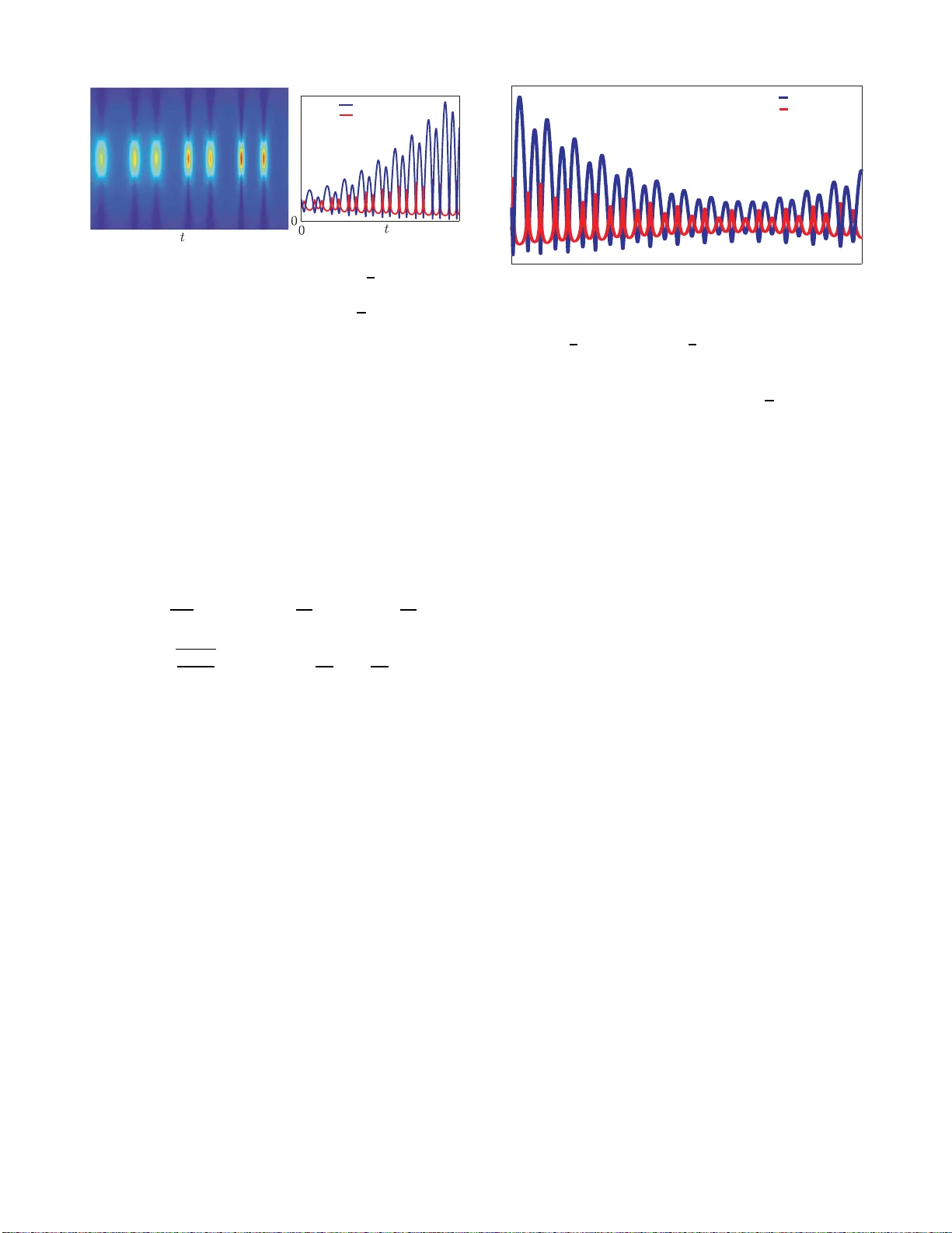
Lo calized nonlinear w a v es in systems with time- and space-mo dulated nonlinearities Juan Belmonte-Beitia 1 , V ´ ıctor M. P ´ erez-Gar c ´ ıa 1 , V a dym V eksler chik 1 , and Vladimir V. Konotop 2 1 Dep artament o de Matem´ at ic as, Escuela T´ ecnic a Sup erior de Ingenier os Industriales, and Instituto de Matem´ atic a Aplic ada a la Ci encia y la Ingenier ´ ıa (IMACI), Universidad de Castil la-L a Mancha, 13071 Ciudad R e al, Sp ain 2 Centr o de F ´ ısic a T e´ oric a e Computacional, Universidade de Lisb o a, Complexo Inter discipl inar, Avenida Pr ofessor Gama Pinto 2, Lisb o a 1649-0 03, Portugal and Dep artamento de F ´ ısic a, F aculdade de Ciˆ encias, Universidade de Lisb o a, Camp o Gr ande, Ed. C8, Piso 6, Lisb o a 1749-016, Portug al. (Dated: October 25, 2018) Using similarit y transformations we construct explicit nontrivial solutions of non linear Schr¨ odinger equations with p oten tials and n onlinearities dep ending on time and on the spatial coordinates. W e present the general theory and use it to calculate explicitly non - trivial solutions such as p erio dic (breathers), resonant or quasiperio dically oscill ating solitons. Some implications to the field of matter-w av es are also d iscussed. P ACS n um b ers: 05.45.Yv, 03.75.Lm, 42.65.Tg Intr o duction .- The co ncept of solitons was intro duce d in the seminal paper by Zabusky and Krusk al [1] to c har- acterize nonlinear so litary wa ves, which emerge fr om the delicate balance b etw een nonlinearity and disp ersion, and preserve their lo calized shap es and v elo cities during prop- agation and after collisions. It was so o n re alized that solitons are remark ably generic ob jects arising in differ- ent contexts and were observed in many e xper imen ts, for example in nonlinear optics starting with the pioneer ing works [2]. Being solutions o f integrable nonlinear wa ve equations, standard solitons app ear usually in transla - tionally inv aria nt sys tems inv olving no nlinearities which depe nd only on the relev ant fields and do not have ex- plicit dep endence on the s pace and time v ariables, b e- cause suc h dep endences t ypica lly break the symmetries of the system. How ever, thos e extra dep endences of the nonlinear interactions op en man y new pra ctical p ossibili- ties for ge ne r ation and control of solitons, what has stim- ulated their study in the las t thirt y years. It was already recognized from the very firs t pap ers [3] that spe c ific de- pendenc ie s of the equation co efficients on the spatial spa- tial co ordina tes a nd on time can pr eserve the in tegr abil- it y . More ov er this g av e an origin to new concepts, like for e x ample, non-a utonomous solitons [4] highly relev ant in nonlinear fib er optics. During the last few years these studies hav e seen an eno rmous reviv al in the context of systems ruled b y nonlinea r Schr¨ odinger (NLS) eq uations bec ause o f their applicatio ns in the mean field theory of Bose-Eins tein condens ates (BECs) [5, 6] a nd in nonlinear optics [4, 7, 8]. In BE C applications, the matter wa ves b eing the nat- ural outcome o f the mean-field des c r iption [5] hav e at- tracted a great deal of in terest in the last years [6]. The p ossibility of using F esch bach resona nces to co n trol the nonlinear ities (see e.g. [9, 10]) has lead to the pro- po sal of man y differe n t no nlinear phenomena induced by the manipulation of the scattering length either in time [11, 12, 13] or in space [14]. In no nlinea r optics, rec e nt de- velopmen ts [1 6] hav e led to the discov ery of a new classes of wav es suc h as the s o-called optica l similariton which arise when the int era ction of nonlinearity , disp ersion and gain in a high-p ow er fibre a mplifier causes the shap e of an ar bitrary input pulse to conv erg e asymptotica lly to a pulse whose shap e is self-simila r. In this letter, w e go b eyond pre vious studies con- sidering s pa ce and time dep endent nonlinearities and constructing differen t types of explicit solutions includ- ing: breathers, reso nan tly oscillating and quas ip erio dic solitary wa ves. W e provide explicit expr e s sions for all those solutions, exploring realistic choices o f no nlineari- ties which are exp erimentally feasible due to the flexible and precise control of the scattering length achiev able in quasi-one-dimensio nal BECs [15] with tunable in ter- actions. Gener al The ory.- W e consider physical s ystems ruled by the NLS equation iψ t = − ψ xx + v ( t, x ) ψ + g ( t, x ) | ψ | 2 ψ , (1) for an unknown complex function ψ ( t, x ) with a po ten tial v ( x, t ) and nonlinear it y g ( x, t ). W e fo cus o n spatia lly lo calized solutions for which lim | x |→∞ ψ ( t, x ) = 0. Our goal is to reduce Eq. (1) to the sta tio nary NLS equa tion µ Φ = − Φ X X + G | Φ | 2 Φ , (2) where Φ ≡ Φ( X ), X ≡ X ( t, x ) is a function to b e de- termined, µ is the eigenv alue of the nonlinear equation, and G is a constant. In this le tter, we ex plo re the case G = − 1, i.e ., fo cusing or attractive nonlinearity . The case G = 1 do es not p ose a n y new challenges and will be studied els e where. T o connect s olutions of E q. (1) with those of Eq. (2) we will use the tra nsformation ψ ( t, x ) = ρ ( t, x ) e iϕ ( t,x ) Φ ( X ( t, x )) . (3) Other simila r it y tr ansformations have been studied fo r NLS equa tions in different contexts [7, 1 7, 18]. 2 8 30 (b) Width Amplitude 0 (a) 12 FIG. 1: [Colo r online] Solution (17), for n = 1, ω 0 = 2, and ε = 0 . 5. Initial d ata for Eq. (11) are ν (0) = √ 2 and ν t (0) = 0. (a) Pseudocolor plot of | ψ ( x , t ) | 2 on the domain x ∈ [ − 3 , 3] (b) Width ν ( t ) (blue line) and amplitude √ γ (red line) vs t . Requiring Φ( X ) to s atisfy Eq. (2) and ψ ( t, x ) to b e a solution of E q. (1) with p otential v ( t, x ) a nd nonlinearity g ( t, x ) we get the set of eq uations ρρ t +  ρ 2 ϕ x  x = 0 ,  ρ 2 X x  x = 0 , X t + 2 ϕ x X x = 0 . Let us take X ( t, x ) = F ( ξ ) , with ξ ( t, x ) = γ ( t ) x + δ ( t ) , (4) where γ ( t ) is a p ositive definite function representing the inv erse of the width of the lo calized solution, and − δ ( t ) /γ ( t ) is the po sition of the center o f mass. After some alg ebra we o btain v ( t, x ) = ρ xx ρ − ϕ t − ϕ 2 x − µ γ 4 ρ 4 , g ( t, x ) = γ 4 ρ 6 , (5) ρ ( t, x ) = r γ F ′ ( ξ ) , ϕ ( t, x ) = − γ t 4 γ x 2 − δ t 2 γ x + α, (6) where α ( t ) is an arbitra ry function of time. Thu s, ch o osing δ ( t ) , γ ( t ) a nd F ( ξ ) (or equiv alen tly ρ ( x, t )) we can generate pairs g ( x, t ) , v ( x, t ) for which the solutions of Eq. (1) can b e obtained from those of E q. (2) using Eqs. (3). W e will use this fact to construct soliton so lutions with an interesting nontrivial b ehavior. L o c alize d nonline arities.- As a fir s t application o f the metho d, we will study the case of lo calized nonlinearities. While the choice of p ossible mo dels is very rich, b ecause of applications the p ossible applications of our re sults to BECs with optica lly controled interactions [10], w e will fo cus on the gaussian sha ped nonlinearity g ( t, x ) = − γ ( t ) exp  − 3 ξ 2  , (7) and the p oten tial including a com bination of harmonic and dip ole traps, which are typical in BE C exp eriments v ( t, x ) = ω 2 ( t ) x 2 + f ( t ) x + h ( t ) − µγ 2 ( t ) exp( − 2 ξ 2 ) , (8) where ω 2 ( t ) = γ 4 +  γ tt γ − 2 γ 2 t  / 4 γ 2 , (9a) f ( t ) =  4 γ 5 δ + δ tt γ − 2 δ t γ t  / 2 γ 2 , (9b) h ( t ) = γ 2 (1 + δ 2 ) − δ 2 t / 4 γ 2 − α t . (9c) 4.5 0 0 40 Width Amplitude t FIG. 2: [Colo r online] Widt h (blue line) and amplitude (red line) versus time of the solution of Eq. (1), given b y Eq. (17) for n = 1, ω 0 = 2, and ε = 0 . 5. Initial data for Eq. (11) given by ν (0) = √ 2 , ν t (0) = − 6 . 125 √ 2. Our choice corre s ponds to ρ ( t, x ) = √ γ exp( ξ 2 / 2) . In the particular ca se wher e δ ( t ) ≡ 0, µ = 0 and α ( t ) = R γ 2 ( t ) dt , we obtain v ( t, x ) = ω 2 ( t ) x 2 , g ( t, x ) = − γ ( t ) e − 3 γ 2 ( t ) x 2 . (10) Thu s, w e hav e a har monic potential and a mo dula ted in time gaussia n nonlinear ity which would cor resp ond in BEC a pplications to a mo dulated laser b eam controlling the interactions optically . In this pap er we focus on non- linearities and p otentials given b y Eq. (10) but many other p ossibilities can b e explor e d using the sa me ideas. Defining ν = 1 / γ we rewr ite Eq. (9a ) in the form ν tt + 4 ω 2 ( t ) ν = 4 /ν 3 , (11) which is the Ermakov-Pinney equation [1 9]. T o discuss explicit s olutions we choose ω 2 ( t ) of the form ω 2 ( t ) = 1 + ε cos( ω 0 t ) , (12) where ε ∈ ( − 1 , 1 ) and 0 6 = ω 0 ∈ R . After so me alg ebra [19], we obtain fr om Eqs. (11) and (12) γ ( t ) =  2 y 2 1 ( t ) + 2( y 2 ( t ) /W ) 2  − 1 / 2 (13) where y 1 , 2 ( t ) are tw o linearly indep e nden t solutio ns of the Mathieu equa tion y tt + 4 ω 2 ( t ) y = 0 (14) and W is their W ronskian. Thu s it is E q. (14) that deter mines the temp o ral dy- namics o f the obtained solutions. Co ns idering different choices of the parameters ω 0 and ε , one can single out three different types of b ehaviors which can b e classified as follows: (i) p erio dic , when ε = 0 or in the frontiers bew tee n the stability and instability r egions o f E q. (14), (ii) r esonant , when ε 6 = 0 and y 1 , 2 ( t ) b elong to a n insta- bilit y region o f E q . (14), and (iii) quasi-p erio dic , when 3 x t x t (a) (b) FIG. 3: [Color online] Plots of | ψ ( x, t ) | 2 for breathing solu- tions of Eq. (1), given by Eqs. (17), for ε = 0 in Eq. ( 12 ), and γ ( t ) giv en by Eq. (19), corresponding to (a) n = 1 (b) n = 2. F or b oth cases, x ∈ [ − 6 , 6], t ∈ [0 , 10] and the initial data for Eq. (11) are ν (0) = √ 2 , ν t (0) = 0. y 1 , 2 ( t ) a r e in the stability regio n. Below we give examples of a ll these cas es. Concerning the so lutio ns of Eq. (2), since µ = 0, Eq. (2) b ecomes Φ ′′ + Φ 3 = 0, and its so lution is given by Φ( X ) = η sn( η X , k ∗ ) / 2 dn( η X , k ∗ ) , (15) with ar bitrary η and k ∗ = 1 / √ 2. W e choose X as X ( t, x ) = Z γ ( t ) x −∞ e − ξ 2 dξ , (16) which takes v alues in (0 , √ π ). This c hoice of X en- sures v anishing of Φ when x → − ∞ . The imp osi- tion o f zero b oundar y condition for x → + ∞ leads to η = 2 nK ( k ∗ ) / √ π where K ( k ) is the elliptic integral. This le a ds to the family of s olutions ψ n = n p γ ( t ) exp  1 2 γ 2 ( t ) x 2 + iϕ ( t, x ))Φ 1 ( nθ ( t, x )  (17) where n = 1 , 2 , ... , ϕ ( t, x ) = − ( γ t / 4 γ ) x 2 + R γ 2 ( t ) dt , Φ 1 ( θ ) = p 2 /π K ( k ∗ ) sn( θ , k ∗ ) / dn( θ , k ∗ ) (18) and θ ( t, x ) = (2 K ( k ∗ ) / √ π ) R γ ( t ) x −∞ dξ e − ξ 2 . It is easy to see that ψ ( x, t ) → 0 when | x | → ∞ in (17), thus they corres p ond to lo calized so lutions. R esonant solitons.- The r espo nse of driven nonlinea r systems to par ametric p erturbations is a field o f interest which has recen tly also be en investigated in the frame- work of the nonlinear dy na mics of BECs [19, 2 0, 21]. Starting with the particula r ca se ω 0 = 2 , in Eq. (12), we observe that for ε 6 = 0 we ar e in the instabilit y r e gion, th us, E q. (17) describ es multisoliton r esonant solutions , since ψ n ( x, t ) p ossesses n − 1 zeros . In Fig. 1 (a ), we plot a reso nan t so lution co r resp onding to n = 1 , with ω 0 = 2. Suc h re sonant soliton ha s an increasing reso nant behaviour. In Fig. 1(b), w e plot its width and ampli- tude versus time. In Fig. 2 , we also plot the width a nd amplitude versus time for the sa me soliton but now with transitory decr easing reso nan t b ehaviour, for n = 1. FIG. 4: [Col or online] Solution of Eq. (1), given by Eq. ( 17), for n = 1, and ω 2 ( t ) = 1 + ε cos( √ 2 t ), with ε = 0 . 5. The initial data for Eq. (11) are ν (0) = 2 3 / 4 and ν t (0) = 0. (a) Pseudocolor plot of | ψ ( x, t ) | 2 (b) W id th ν ( t ). It is rema rk able that we a r e able to construct explicit resonant so litons in a very co mplicated s c enario including a loca lized pulsating nonlinearity and a parametr ically mo dulated trap a long the longitudinal direction. Our so- lutions pr ovide the first explic it res onant solution in a parametrica lly mo dulated one dimensio nal BE C. A sim- ilar r e sonant b ehavior was observed in Ref. [21] when driving a BEC, with p ositive sc a ttering length, along the transverse dir e c tion. W e hav e also studied the stability of these m ultisoliton solutions g iv en by Eq. (17) b y computing numerically their evolution under finite amplitude per turbations. W e hav e found that n = 1, which co rresp onds to the gr ound state, is a s table solution while hig he r solitons are un- stable (sma ll p erturba tions take the solution far from its original pr o file). Br e athing solitons.- When ε = 0 , ω ( t ) = 1, a nd then γ ( t ) = √ 2  1 + 3 cos 2 (2 t )  − 1 / 2 (19) is per io dic. Then, the so lutions giv en by Eq. (17) ar e explicit multisoliton br e athing solutions . In Fig. 3 , we plot so me of them corr e spo nding to n = 1 , 2. Only fo r n = 1 (the gro und state) the breathing soliton is stable. Quasip erio dic solutions.- In o rder to give an exa mple of a quasip erio dic solution o f Eq. (1) we cho ose ω 0 = √ 2 in Eq. (12) ensur ing that the solutions y 1 , 2 ( t ) of the Math- ieu equa tion (14) b elong to the stability region. Then Eq. (12) has t wo incommensurable frequencies. In this wa y , γ ( t ), is a quasip erio dic solution and the solutions (17) show a quasip erio dic b ehaviour. An example o f this behavior is shown in Fig. 4. Using Eqs. (17), w e can also constr uct multisoliton quasip erio dic solutions . Moving s olitons.- As a fina l example of the many p ossi- ble solutions which ca n b e c o nstructed using this method, we will present solutions of Eq. (1) when the cen tre of mass of the soliton mov es with non-z ero velocity . T o do so, w e set f ( t ), in Eq. (9b) equal to zero , with δ 6 = 0 which leads to the following equa tion for δ ( t ), δ tt − 2 ( γ t /γ ) δ t + 4 γ 4 δ = 0 . (20a) 4 FIG. 5: [Color online] Pseudocolor plots of sol utions of Eq. (1), when the centre of mass of t h e soliton mov es with non- zero v elo cit y . (a) Quasip eriodic solution, with x ∈ [ − 3 , 3], t ∈ [0 , 40], fo r ε = 0 . 6 and ν ( 0) = (2 √ 2) 1 / 2 , ν t (0) = 0. (b) Resonant increasing solution, with x ∈ [ − 6 , 6], t ∈ [0 , 40] for ε = 0 . 3 and ν (0) = √ 2 , ν t (0) = 0. In this situation, the p otent ial v and the nonlinearity g are s till given by E q. (10) by just taking α t = γ 2 (1 + δ 2 ) − δ 2 t / 4 γ 2 . (20b) F o rtunatelly , Eqs . (20) can b e solved to ge t δ ( t ) = δ ∗ cos(2 τ ( t )) , α ( t ) = τ ( t ) + 1 4 δ 2 ∗ sin(4 τ ( t )) , (21) where τ ( t ) = R γ 2 ( t ) dt , and δ ∗ is a n arbitrary constant. Hence, we ca n again obtain breathers , resonant solutions and quasip erio dic solutions while, at the same time the center of ma ss of the soliton moves in a co mplex wa y according to Eq. (21). As exa mples, in Fig. 5, we show quasip erio dic [Fig. 5(a)] and resona n t so litons [Fig. 5(b)] while the center of mas s mov es accor ding to E q. (21). Conclusions.- W e have cons tructed explicit solutions of nonlinea r Schr¨ odinger equatio ns in co mplicated yet re- alistic scenar ios w ith s patially inhomogene o us and time depe ndent potentials a nd no nlinearities. Althoug h the range of no nlinearities and p otentials for which this can be do ne is very wide, we hav e fo cused our study in mo d- ulated harmonic p otentials a nd lo caliz e d nonlinearities. W e ha ve explicitly ca lc ula ted brea thers, resonant soli- tons, qua siper io dic solitons and solutions with nontrivial motion of the cen ter o f mass, related to different situ- ations of physical interest in the fie ld of Bose-E instein condensates. The ideas con tained in this pa per can also be applied to study m ulticomp onent systems, nonlinea r optical sys tems, higher - dimensional situations, etc., and may help in the design of p otentials and nonlinear ities to control the dynamics of Bose-E instein co ndensates. This work has b een pa rtially supp orted by gra n ts FIS2006- 0 4190 (Minister io de Educaci´ o n y Ciencia, Spain), P CI08-009 3 (Jun ta de Co m unidades de Ca stilla- La Ma nc ha, Spain), and POCI/FIS/5 6 237/2 004 (Eur o- pea n Pr ogram FEDER a nd FCT, Portugal). [1] N. J. Zabusky and M. D. Krusk al, Phys. Rev. Lett., 15 , 240 (1965). [2] A. Hasega wa and F. T app ert, Appl. Phys. Lett ., 23 , 142 (1973); ibidem 23 , 171 (1973). [3] H.-H . Chen and C.-S. Liu, Phys. Rev. Lett. 37 , 693 (1976); M. Brusc hi, D. Levi, and O. R agnisco, Nuov o Cimen to, 53 , 21 (1979); R. Scharf and A. R . Bishop, Phys. Rev. A 43 , 6535 (1991); V. V. Konotop, O. A. Chub yk alo, and L. V´ azquez, Phys. Rev. E 48 , 563 (1993). [4] V.N. S erk in, A. Hasega wa, and T.L. Belyaev a, Phys. R ev. Lett., 98 , 074102 (2007). [5] L. P . Pitaevskii, and S. Stringari, Bose-Einstein Conden- sation , Oxford Universit y Press, Oxford (2003). [6] Emer gent Nonli ne ar Phenomena in Bose-Einstein Con- densates: The ory and Exp erim ent , P .G. Kevrekidis, D.J. F rantzesk akis, and R. Carretero-Gonz´ alez, Ricardo (Eds.), Springer, V ol. 45 (2008). [7] V.N. Serkin, and A. Hasega w a, Phys. Rev . Lett, 85 (2000) 4502; JETP Lett. 72 , 89 (2000); S el T op. Quant. Electron, 8 , 418 (2002); V.N. Serk in, A. Hasegaw a, and T. L. Belyaev a, Phys. Rev . Lett. 92 , 199401 (2004) [8] Y. Kivshar and G. P . Agraw al, Optic al Soli tons: F r om fib ers to Photonic crystals , A cademic Press (2003). [9] S. Inouye, et al. , N ature 392 , 151 (1998). [10] M. Theis, et al . , Phys. Rev. Lett. 93 , 123001 (2004). [11] B. A. Malomed, Sol iton Management in Perio di c Sys- tems , Springer (New Y ork, 2006). [12] F. Kh. Ab du llaev, et al. , Phys. Rev . Lett. 90 , 230402 (2003); V . M. P´ erez-Garc ´ ıa, V. V. Konotop, and V. A. Brazhnyi, Phys. Rev. Lett. 92 , 220403 (2004). [13] H. Saito and M. Ueda, Phys. Rev. Lett. 90 , 040403 (2003); F. Kh . Ab dullaev, et al . , Phys. Rev. A 67 , 013605 (2003); G. D . Montesinos , V. M. P´ erez-Garc ´ ıa and P . T or- res, Physica D 191 , 193 (2004); V. V. Konotop and P . P acciani, Ph ys. Rev. Lett. 94 , 240405 (2005); V . Zhar- nitsky and D. Pel inovsky , Chaos 15 , 037105, (2005); A. Itin, T. Morishita, and S. W atanab e, Phys. Rev. A, 74 , 033613 (2006). [14] M. I. Ro das-V erd e, H. Michinel and V. M. P ´ erez-Garc ´ ıa, Phys. Rev. Lett . 95 (2005) 153903; H. Sak aguchi and B. Malomed, Phys. Rev. E 72 , 046610 (2005); G. Theocharis, et al. , Phys. Rev. A 72 , 033614 (2005); F. K. A bd ullaev and J. Garnier, i bid. , 72 , 06160 5(R) (2005); J. Garnier and F. K. Abd ullaev, ibid. 74 , 013604 (2006); M. A. Porter, et al . , Physica D , 229 , 104 (2007); J. Belmon te-Beitia, et al. , Phys. Rev . Lett. 98 , 064102 (2007). [15] The relations a s ≪ a ⊥ ≪ λ ≪ a k , where a s is the scat- tering length, a ⊥ , a k , are the transverse and longitudinal trap lengths, and λ is a c haracteristic spatial scale of the w av e pac ket, define the region in whic h the one dimen- sional approac h describ es correctly the p hysics inv olv ed. [16] S. A. Ponomarenk o and G. P . Agraw al, Phys. Rev. Lett., 97 , 013901 (2006 ); J. M. Dudley et al , N ature Physics, 3 , 597 (2007). [17] V. M. P ´ erez-Garc ´ ıa, P . J. T orres, and V. V. K onotop, Physica D 221 , 31 (2006). [18] S. Chen and L. Y i, Phys. Rev. E 71 , 016606 . (2005) [19] V. M. P´ erez-Garc ´ ıa, P . J. T orres and G. D. Montesinos, SIAM J. Appl. Math. 67 , 990 (2007). [20] K. Staliunas, S. Longhi, and G. J. de V alc´ arcel, Ph ys. Rev. Lett. 89 , 210406 (2002); Y u. V. Bludov and V. V. Konotop, Phys. Rev. A 75 , 053614 (2007); [21] P . Engels, C. Atherton, and M. A. Hoefer, Phys. R ev. Lett. 98 , 095301 (2007).