Perturbation theory for bright spinor Bose--Einstein condensate solitons

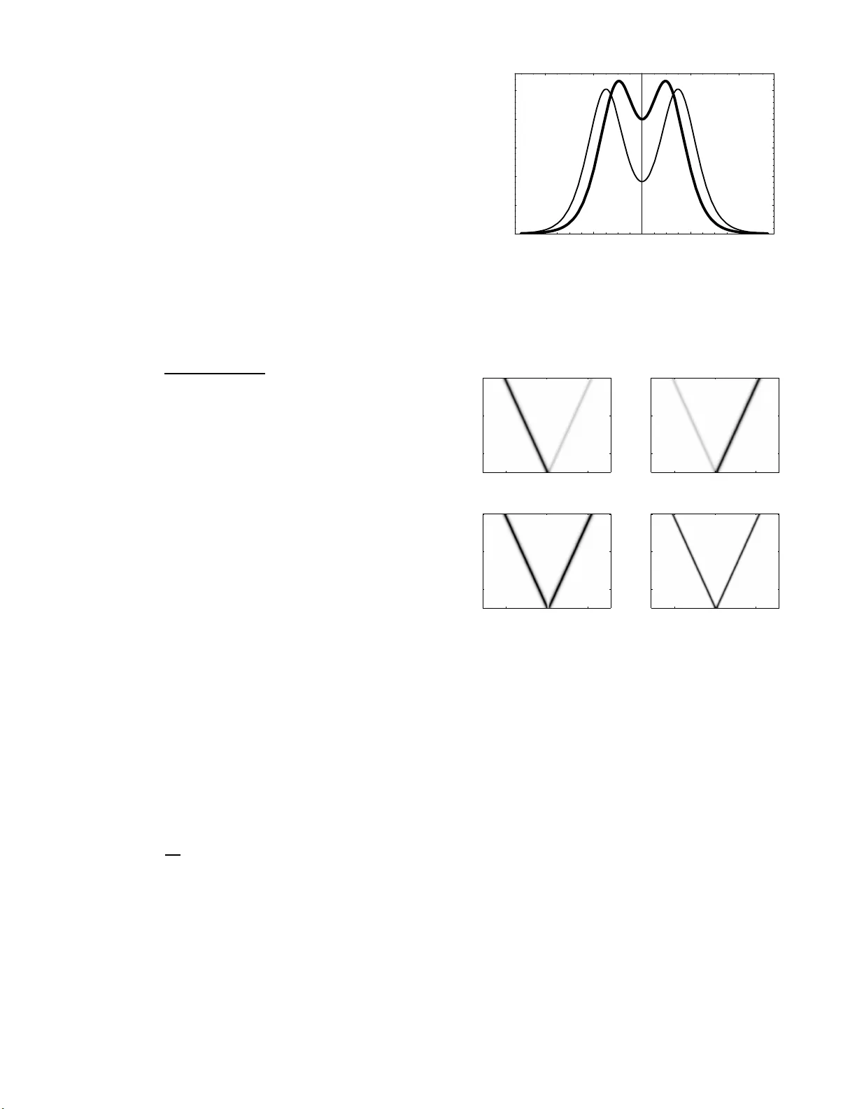
P erturbation theory for brigh t spinor Bose–Einstein condensa te solitons Evgeny V. Doktorov, 1, ∗ Jiandong W ang, 2 , † and Jianke Y ang 2 , ‡ 1 B.I. Step anov Institute of Physics, 220072 Minsk, Belarus 2 Dep artment of Mathematics and Statistics, Univer sity of V ermont, Bur lington, VT 05401 W e develop a p erturbation theory for b ri ght solitons of the F = 1 integrable spinor Bose-Einstein condensate (BEC) mo del. The formalism is based on u sing the Riemann- Hilbert problem an d provides the me ans to analytically calculate ev olution of the soliton parameters. Both rank-one and rank-tw o soliton solutions of the mod el are obtained. W e prov e equiva lence of the rank-one soliton and the ferromagnetic rank-tw o soliton. T aking into account a splitting of a p erturb ed p ol ar rank-tw o sol iton into tw o ferromagnetic solitons, it is sufficient to elab orate a p erturbation theory for the rank-one solitons only . T reating a small d eviatio n from the integ rabilit y condition as a p erturbation, we d escr ib e th e spinor BEC soliton dynamics in the adiabatic approxima tion. It is show n th at the solito n is quite robust against such a perturb atio n and preserves its velocit y , amplitude, and p opulation of different spin comp onen ts, only the soliton frequency acquires a small shift. Results of numerical simula tions agree well with the an alyt ical pred icti ons, demonstrating only slight soliton p rofi le deforma tion. P ACS num b ers: 03.75 .Lm, 03.75.Mn, 02.30.Ik I. INTRO DUCTION Bright a nd dark s olitons in quasi-one- dimensional Bose–E instein condensates (BECs), observed exp erimen- tally [1, 2, 3, 4], are exp ected to b e impor ta n t for v arious applications in atom optics [5], including atom interfer- ometry , atom lasers, and coherent a tom tra nsport. Re- cent exp erimental and theoretical adv ances in BEC so li- ton dyna mics ar e reviewed in Refs. [6, 7, 8 ]. Spinor BEC of a lk ali atoms [9, 10] with a purely opti- cal confinement, along with the tw o-comp onen t co nden- sate [11, 12, 13], represents an example of the condensate with int ernal de g rees of fr eedom which endow the soli- tons with vectorial pro perties. Modulational instability in the spinor BEC mo del was investigated in Ref. [14], and some exact solutions and their stability were stud- ied in Ref. [15]. V ector gap solitons a nd self-tra pp ed wa ves were iden tified in the spinor BEC mo del loaded int o one-dimensional optical lattice p oten tial [1 6]. Re- cently bright-dark s o liton complexes in this mo del have bee n found [17] b y r educing it to the co mpletely inte- grable Y a jima-Oik aw a sys tem [1 8 ]. W adati and c o-w orkers found [19] that the three- comp onen t nonlinea r equa tions describing the B EC with the hyper fine spin F = 1 a dmit the reduction to another int egrable mo del – the 2 × 2 matrix nonlinea r Schr¨ odinger (NLS) equation, after imp osing a constra in t on the con- densate parameters. Both bright [2 2] and dark [23] soli- tons p ossessing pr operties of true so litons of int egrable equations hav e b een found. The formalis m of the inverse scattering transform for the matrix NLS equatio n under non-v anishing b oundary conditions was develop e d in Ref. ∗ Electronic address: doktoro v@dragon.bas-net.b y † Electronic address: jwang @cems.uvm.edu ‡ Electronic address: jyan g@cems.uvm.edu [24] and extended in Ref. [25] to desc r ibe bright spinor BEC soliton dynamics on a finite background. The full- time description of the mo dulational ins tabilit y develop- men t in the integrable spinor BEC mo del was given b oth nu merically [15] and analytically [26]. Int egrable mo dels provide a very useful pr o v ing ground for testing new a nalytical and nu merical approaches to study such a complicated system a s the spino r BEC. At the same time, the int egrability conditions impo se sp e- cific r estrictions on the par ameters o f the mo del which can conflict with actual exp erimen tal s ettings, despite the fact that the effective in teraction b et ween atoms in BEC can be tuned, to so me extent, by the o ptically induced F eshbac h res onance [20, 21]. Bes ides, in ex p eriment it is impo ssible to exactly hold the conditions b et ween param- eters which assure integrability of the mo de l. Therefor e, sufficiently genera l analytica l r esults concerning the full (nonint egrable) mo del with realistic parameters would be of imp ortance. As a step in this direction, in the prese n t pap er w e de- velop a p erturbation theor y for the integrable spinor BE C mo del. Evidently , small dis tur bance of the in tegrability condition can b e considered as a p erturbation of the inte- grable mo del. Our formalism is based o n the Riema nn– Hilber t (RH) problem asso ciated with the spinor BEC mo del. The main adv antage of the prop osed metho d is its algebr aic nature, a s distinct from the metho d using the Gel’fand– Levitan in tegral equations [27]. The a p- plication of the RH problem for treating per turbed soli- ton dynamics goe s back to Refs. [28, 29]. The mo d- ern version of the p erturbation theory in terms of the RH problem has b een develop ed in a series of pap ers [30, 31, 32, 33 , 34], with its most genera l formulation in Ref. [35]. Another version of the soliton p erturbation theory (the direct p erturbation theory) has b een devel- op ed on the ba s is of expanding p erturbed s o lutions into squared eigenfunctions of the linearized soliton equations [36, 37]. 2 As w as shown b y W adati and co-workers [19, 22], bright solitons in the integrable spinor BE C mo del c a n exist in tw o spin states – ferroma gnetic (no n- zero total spin) and p olar (zero to tal spin). E nergy of the p olar soliton is grea ter than that of the ferro magnetic s oliton. Moreov er, the p olar soliton demonstrates a tw o-humped profile in a wide range of its par ameters. Our num erical simulations revealed that the p olar soliton is unstable un- der the action of a p erturbation o f a ra ther genera l form and s plits in to tw o ferroma gnetic solitons. This fact is crucial for the development of a p erturbation theory for spinor BE C solito ns. The pap er is or ganized as follows. After formulating the mo del in Sec. I I, we in tro duce in Sec. I II ana lytic solutions of the as sociated sp ectral problem, in order to for m ulate in Sec. IV the RH pr oblem. Solving this problem, we derive in Sec. V brig h t soliton solutions of the int egrable spinor BEC mo del, bo th for the rank- one and rank - t wo pro jectors. The ra nk-one so liton is char- acterized by the familiar hyp e rbolic secant pr ofile, while the rank-tw o soliton has a more complicated for m [19]. Two t yp es of the ra nk-t wo solutions are exactly ferro - magnetic and p olar solitons. W e pr o ve tha t the fer ro- magnetic r ank-t w o s o liton is equiv ale nt to the rank-o ne soliton. In vir tue of the fact that the p erturbed pola r soliton splits into tw o r ank-t wo ferro magnetic s o litons, it is sufficient to develop a p erturbation theo ry for the rank-one soliton only . This is pe r formed in Sec. VI. W e der iv e evolution equations for the s oliton par ameters which exactly account for the per turbation a nd s erv e as the gener ating equations for iter ations. Se c tion VI I con- tains a description of the soliton dyna mics in the a dia- batic approximation of the p erturbation theor y . W e show analytically that a ferroma gnetic soliton is quite robust against a s mall disturba nce o f the in tegrability co ndi- tion, the only manifesta tion of the p erturbation action is a minor shift o f the solito n frequency . Numerical simula- tions of the p e r turbed spinor BEC equa tions are in clo se agreement with the ana lytical pr edictions r e v ea ling only a small s o liton shap e dis tortion and little p erturbation- induced ra diation. Sectio n VI II concludes the pap er. II. MODEL W e c o nsider an effective one-dimensional BEC tr apped in a p encil-shaped region elong ated in the x dir ection and tig h tly co nfined in the transversal directions. The assembly of atoms in the h yp erfine spin F = 1 state is describ ed by a vector order parameter Φ → ( x, t ) = (Φ + ( x, t ) , Φ 0 ( x, t ) , Φ − ( x, t )) T , where its co mponents cor- resp ond to three v a lues of the spin pro jection m F = 1 , 0 , − 1. The functions Φ ± and Φ 0 ob ey a sys tem of coupled Gros s–Pitaevskii equa tions [22, 3 8] i ~ ∂ t Φ ± = − ~ 2 2 m ∂ 2 x Φ ± + ( c 0 + c 2 )( | Φ ± | 2 + | Φ 0 | 2 )Φ ± + ( c 0 − c 2 ) | Φ ∓ | 2 Φ ± + c 2 Φ ∗ ∓ Φ 2 0 , (2.1) i ~ ∂ t Φ 0 = − ~ 2 2 m ∂ 2 x Φ 0 + ( c 0 + c 2 )( | Φ + | 2 + | Φ − | 2 )Φ 0 + c 0 | Φ 0 | 2 Φ 0 + 2 c 2 Φ + Φ − Φ ∗ 0 , where the co ns tan t parameter s c 0 = ( g 0 + 2 g 2 ) / 3 and c 2 = ( g 2 − g 0 ) / 3 control the spin-indep endent and spin- depe ndent interaction, res pectively . The co upling con- stant g f ( f = 0 , 2) is given in terms o f the s -wa v e scat- tering le ngth a f in the channel with the total hyperfine spin f , g f = 4 ~ 2 a f ma 2 ⊥  1 − C a f a ⊥  − 1 . Here a ⊥ is the size of the transverse gro und sta te, m is the ato m mass, and C = − ζ (1 / 2) ≈ 1 . 4 6 . It was noted in [19] that Eqs . (2.1) are reduce d to a n int egrable sys tem under the co nstrain t c 0 = c 2 ≡ − c < 0 . (2.2) The negative c 2 means that we consider the ferromag - netic gr ound state of the spinor BE C with attractive in- teractions. The condition (2.2 ), b eing written in terms of g f as 2 g 0 = − g 2 > 0, imp oses a cons train t on the scattering lengths: a ⊥ = 3 C a 0 a 2 / (2 a 0 + a 2 ). Redefin- ing the function Φ → as Φ → → ( φ + , √ 2 φ 0 , φ − ) T , nor malizing the co ordinates as t → ( c/ ~ ) t and x → ( √ 2 mc/ ~ ) x , and accounting for the co nstrain t (2.2), we o bta in a reduce d system of equations in a dimensionles s form: i∂ t φ ± + ∂ 2 x φ ± + 2  | φ ± | 2 + 2 | φ 0 | 2  φ ± + 2 φ ∗ ∓ φ 2 0 = 0 , (2.3) i∂ t φ 0 + ∂ 2 x φ 0 +2  | φ + | 2 + | φ 0 | 2 + | φ − | 2  φ 0 +2 φ + φ ∗ 0 φ − = 0 . After ar r anging the co mp onents φ ± and φ 0 int o a 2 × 2 matrix Q , Q =  φ + φ 0 φ 0 φ −  , (2.4) we transfor m Eqs. (2.3) to the integrable matr ix NLS equation i∂ t Q + ∂ 2 x Q + 2 QQ † Q = 0 . (2.5) The ma tr ix NLS eq ua tion (2.5) app ears a s a co mpatibil- it y condition of the system of linear equations [27] ∂ x ψ = ik [Λ , ψ ] + ˆ Qψ , (2.6) ∂ t ψ = 2 ik 2 [Λ , ψ ] + V ψ , (2.7) 3 where Λ = diag ( − 1 , − 1 , 1 , 1 ), ˆ Q =  0 Q − Q † 0  , V = 2 k ˆ Q + i  QQ † Q x Q † x − Q † Q  , (2.8) and k is a sp ectral pa rameter. E q uation (2.6) (the sp ec- tral pr o blem) enables us to deter mine initial sp ectral data from the known p otential ˆ Q 0 , while Eq. (2.7) g o verns the tempo ral evolution of the sp ectral data. A new so lution of Eq. (2.5) [and he nc e of the BEC equa tions (2.3)] is ob- tained as a r esult o f the recons tr uction of the p oten tial ˆ Q from the time- de p endent sp ectral data. II I. JOST AND ANAL YT IC SOLUT IO NS T o determine the s p ectral data , we introduce matrix Jost solutions J ± ( x, k ) of the sp ectral pro blem (2.6) by means of the asymptotes J ± → 1 1 as x → ±∞ . Since trΛ = 0, we have det J ± = 1 for all t . Being solutions of the first-o rder equation (2.6), the Jost functions ar e not indep enden t but are interconnected b y the sc a ttering matrix S : J − = J + E S E − 1 , E = exp( ik Λ x ) , det S = 1 . (3.1) Besides, the Jo s t s o lutions and the scattering matrix ob ey the inv olution prop ert y . Indeed, since the p otential ˆ Q is anti-Hermitian, we obtain J † ± ( k ∗ ) = J − 1 ± ( k ) . (3.2) Similarly for the s c a ttering ma trix: S † ( k ) = S − 1 ( k ) . (3.3) Note that the scattering matrix is defined for real k . F or the subsequent analysis , analytic prop erties o f the Jost solutions are of primary imp ortance. Let us repr e- sent the matrix J ost s olution J a s a collection of columns: J = ( J [1] , J [2] , J [3] , J [4] ), and consider the first column. Rewriting the spectr a l eq ua tion (2 .6) with the corre- sp onding b oundary conditions in the for m o f the V olterra int egral equations, we obta in a closed system of equatio ns for entries of the first column: J − 11 = 1 + Z x −∞ d x ′ ( φ + J − 31 + φ 0 J − 41 )( x ′ ) , J − 21 = Z x −∞ d x ′ ( φ 0 J − 31 + φ − J − 41 )( x ′ ) , J − 31 = − Z x −∞ d x ′ ( φ ∗ + J − 11 + φ ∗ 0 J − 21 )( x ′ ) e 2 ik ( x − x ′ ) , J − 41 = − Z x −∞ d x ′ ( φ ∗ 0 J − 11 + φ ∗ − J − 21 )( x ′ ) e 2 ik ( x − x ′ ) . The last t wo integrands p oin t out that the column J [1] − is analytic in the upp er half-plane C + , where Im k > 0, and contin uous on the rea l axis Im k = 0. This can b e proved in the same wa y a s for the scalar NLS equatio n, under the condition of sufficiently fast decreas e o f the p oten tial ˆ Q at infinit y . Similarly we obtain that the co lumn J [2] − is a nalytic in C + as well, while the tw o other columns J [3] − and J [4] − are analytic in the low er half-plane C − and contin uous o n the real axis Im k = 0. As regar ds the matrix solution J + , its firs t and seco nd columns J [1] + and J [2] + are a nalytic in C − , while the third and forth ones J [3] + and J [4] + are a nalytic in C + . Ther efore, the matrix function ψ + =  J [1] − , J [2] − , J [3] + , J [4] +  (3.4) solves the spe ctral equation (2.6) and is analytic as a whole in C + . It is not difficult to see from Eqs. (3.1) and (3.4) that the ana lytic solution ψ + can be expres sed in terms of the Jost functions and some entries of the scatter ing matrix: ψ + = J + E S + E − 1 = J − E S − E − 1 , (3.5) where S + ( k ) =    s 11 s 12 0 0 s 21 s 22 0 0 s 31 s 32 1 0 s 41 s 42 0 1    , S − ( k ) =    1 0 s ∗ 31 s ∗ 41 0 1 s ∗ 32 s ∗ 42 0 0 s ∗ 33 s ∗ 43 0 0 s ∗ 34 s ∗ 44    . (3.6) In writing the ex pression for S − we use the involution (3.3). These upp er and low er blo ck-triangular matrices S ± factorize the scattering matrix [39]: S S − = S + . Be- sides, it follows fro m Eq. (3.5) a nd det J ± = 1 that det ψ + = m (2) + = m (2) ∗ − , (3.7) where m (2) + ( m (2) − ) is the second-or der principa l upp e r (low er ) minor of the scatter ing matrix. T o obtain the analytic co un terpa r t of ψ + in C − , we consider the adjoint s pectral eq uation ∂ x K ± = ik [Λ , K ± ] − K ± ˆ Q (3.8) with the asymptotic conditions K ± → 1 1 at x → ± ∞ . The inv erse matrix J − 1 can s erv e as a s olution of the adjoint equation (3.8). Now we write a c lo sed system of integral equations for rows o f the matric e s K ± . F o r example, the first row K − [1] ob eys the equations K − 11 = 1 + Z x −∞ d x ′ ( φ ∗ + K − 13 + φ ∗ 0 K − 14 )( x ′ ) , K − 12 = Z x −∞ d x ′ ( φ ∗ 0 K − 13 + φ ∗ − K − 14 )( x ′ ) , K − 13 = − Z x −∞ d x ′ ( φ + K − 11 + φ 0 K − 12 )( x ′ ) e − 2 ik ( x − x ′ ) , K − 14 = − Z x −∞ d x ′ ( φ 0 K − 11 + φ − K − 12 )( x ′ ) e − 2 ik ( x − x ′ ) . 4 It is seen that the r o w K − [1] is analytic in C − . Similarly , the second r o w K − [2] is analytic in C − , too , and the rows K − [3] and K − [4] are analytic in C + . F o r the matrix solution K + we find that the r o ws K +[1] and K +[2] are analytic in C + , while K +[3] and K +[4] are analytic in C − . Therefore, the matrix function ψ − 1 − =  K − [1] , K − [2] , K +[3] , K +[4]  T (3.9) solves the adjoint equation (3.8) and is ana lytic as a whole in C − . Similar to ψ + , the function ψ − 1 − is ex- pressed in terms o f the Jost solutions a nd the scattering matrix: ψ − 1 − = E T + E − 1 J − 1 + = E T − E − 1 J − 1 − , (3.10) where the matrices T ± , T + =    s ∗ 11 s ∗ 21 s ∗ 31 s ∗ 41 s ∗ 12 s ∗ 22 s ∗ 32 s ∗ 42 0 0 1 0 0 0 0 1    , T − =    1 0 0 0 0 1 0 0 s 31 s 32 s 33 s 34 s 41 s 42 s 43 s 44    , provide o ne mo re factor ization o f the sca ttering matr ix: T − = T + S . As in E q. (3.7 ), we can wr ite det ψ − 1 − = m (2) ∗ + = m (2) − . (3.11) Note that the analy tic solutions satisfy the inv olution prop ert y a s well: ψ † + ( k ) = ψ − 1 − ( k ∗ ) . (3.12) This pr operty can be taken as a definition of the a nalytic function ψ − 1 − from the known ana lytic function ψ + . IV. THE RIEMA NN- HILBER T PROBLEM Hence, we co nstructed tw o ma trix functions ψ + and ψ − 1 − which are analytic in complementary domains of the complex plane and co njugate on the real line. Indeed, it follows from Eqs. (3.5) and (3.10) that ψ ± ob ey the relation ψ − 1 − ( k ) ψ + ( k ) = E G ( k ) E − 1 , Im k = 0 , (4.1) where G = T + S + = T − S − =    1 0 s ∗ 31 s ∗ 41 0 1 s ∗ 32 s ∗ 42 s 31 s 32 1 0 s 41 s 42 0 1    . (4.2) Equation (4.1) deter mines a matrix Riemann-Hilb ert problem, i.e. a problem of the ana lytic factorizatio n of a nondegenera te matrix G in (4.2), given on the rea l line, int o a pro duct of tw o matrices which a re analytic in c o m- plement ary domains C ± . The RH problem (4.1) needs a normalizatio n condition, which is usually taken as ψ ± ( x, k ) → 1 1 at | k | → ∞ . (4.3) The analytic matrix functions ψ ± can b e treated as a result of a nonlinea r mapping b et ween the p oten tial ˆ Q ( x ) and a set o f the sp ectral data which uniquely char- acterizes a solutio n of the RH problem (4.1) a nd (4.3). Conv er sely , the p otential can b e re c o nstructed from an asymptotic expansio n of ψ ± ( x, k ) for lar ge k . Indeed, writing ψ ± as ψ + ( x, k ) = 1 1 + k − 1 ψ (1) + + O ( k − 2 ) , ψ − 1 − ( x, k ) = 1 1 + k − 1 ψ (1) − + O ( k − 2 ) and ins erting these expa nsions in to Eqs . (2.6) and (3.8), we obtain ˆ Q = − i [Λ , ψ (1) + ] = i [Λ , ψ (1) − ] . (4.4) Hence, having solved the RH pr oblem, we can find solu- tions of the BE C equatio ns. In general, the matrices ψ + and ψ − 1 − can hav e zer o s k j and κ l in the corres ponding doma ins of a nalyticit y: det ψ + ( k j ) = 0, k j ∈ C + , and det ψ − 1 − ( κ l ) = 0, κ l ∈ C − . In virtue o f the inv olution (3.12), we obta in κ l = k ∗ l and equal num b er N of zeros in b oth ha lf-planes. The corre- sp onding RH problem is said to b e nonregula r , or the RH problem with zer os. They a re zero s of the RH problem that deter mine soliton solutions of the BEC equations . It is s een from Eq s . (3.6) and (3 .7 ) that zeros of ψ + nu llify 2 × 2 minors o f ψ + . Hence, the r ank of ψ + ( k j ) can b e equal to one or tw o . It means in turn that there exist one ( | 1 j i ) or tw o ( | 1 j i and | 2 j i ) four- component eig e n vectors that co r respond to zero eig en v a lue of ψ + ( k j ): ψ + ( k j ) | 1 j i = 0 for rank ψ + ( k j ) = 1 , (4.5) ψ + ( k j ) | 1 j i = ψ + ( k j ) | 2 j i = 0 for rank ψ + ( k j ) = 2 . The g eometric multiplicit y o f k j is equal to the dimen- sion o f the null space of ψ + ( k j ) (1 or 2 in our cas e). In this pap er, we only consider the cas e of zero s k j with its geometric multiplicit y equa l to the algebra ic multiplicit y [which is the order of the zer o k j in det ψ + ( k )]. Note that the solution of the RH pro blem for the genera l c a se of zeros with unequa l geo metric and algebraic multiplic- ities was elab orated in Ref. [40]. W e will so lve the matrix non-r egular RH problem with zer o s k 1 and k ∗ 1 by means of its reg ularization, i.e. b y extracting fr om ψ + and ψ − 1 − rational factors that are resp onsible for the a pp earance of zer os. Hence, det ψ + ( k 1 ) = 0 [and corr espondingly det ψ − 1 − ( k ∗ 1 ) = 0]. W e need a r ational matrix function Ξ − 1 ( x, k ) which ha s a po le in the p oin t k 1 . Let us take Ξ − 1 ( x, k ) in the form Ξ − 1 ( x, k ) = 1 1 + k 1 − k ∗ 1 k − k 1 P ( r ) , where P ( r ) = r X l,m =1 | l i ( M − 1 ) lm h m | , (4.6) 5 h m | = | m i † due to inv olution, and r = rank ψ + ( k 1 ). P ( r ) is a pro jector of ra nk r , ( P ( r ) ) 2 = P ( r ) , and entries o f the r × r matrix M ar e determined by ( M ) lm = h l | m i = 4 X a =1 ( l ) ∗ a ( m ) a . In the appropria te basis the pro jector is represented as P (1) = diag(1 , 0 , 0 , 0) or P (2) = diag(1 , 1 , 0 , 0). This yields det Ξ − 1 =  k − k ∗ 1 k − k 1  r . Therefore, the pro duct ψ + ( x, k )Ξ − 1 ( x, k ) is reg ular in k 1 . In the same wa y , the regula rization of ψ − 1 − in the p oin t k ∗ 1 is p erformed by the r ational function Ξ( x, k ) = 1 1 − k 1 − k ∗ 1 k − k ∗ 1 P ( r ) , (4.7) which provides the pro duct Ξ ψ − 1 − to b e r egular in k ∗ 1 . Therefore, the analytic functions ar e factorized as ψ + ( k ) = e ψ + ( k )Ξ( k ) , ψ − 1 − ( k ) = Ξ − 1 ( k ) e ψ − 1 − , (4.8) with holomor phic functions e ψ ± which determine the reg - ular (without zeros) RH proble m: e ψ − 1 − ( k ) e ψ + ( k ) = Ξ( k ) E G ( k ) E − 1 Ξ − 1 ( k ) , k ∈ Re . (4.9) F or sev eral pa ir s of ze ros ( k j , k ∗ j ), j > 1, the regu- larization of the RH problem ca n be p erformed in the same step-by-step manner , with the appropr iate defini- tion o f the eig en vectors within each step. Howev er , for practical calcula tion of N -soliton e ff ects it is m uch more conv enie nt to expa nd a pro duct of rationa l facto r s into simple fractions, thereby transforming the pr oduct-type expression into a sum-type one [3 2, 4 0]. It is easy to find the c o ordinate dep endence of the eigenv e ctors. Indeed, differentiating (4.5) in x and in t with j = 1 and accounting Eqs. ( 2.6) a nd (2.7 ) gives ( | l 1 i ≡ | l i ) ∂ x | l i = ik 1 Λ | l i , ∂ t | l i = 2 ik 2 1 | l i , (4.10) with l = 1 for r ank o ne , a nd l = 1 , 2 for rank tw o. Hence, | l i = exp( ik 1 Λ x + 2 ik 2 1 Λ t ) | l (0) i , (4.11) where | l (0) i is the co ordinate-free four-dimensional vec- tor. Zeros k j and vectors | l (0) j i comprise the discrete data of the RH problem that determine the solito n conten t of a solution of the BEC equations. The contin uous data are characterize d by the off-blo ck-diagonal pa rts o f the matrix G ( k ) (4.2), k ∈ Re, and are resp onsible for the radiation comp onen ts. In the following se ction we co n- cretize the ab o ve relations to obtain one- soliton solutions of E qs. (2.3). V. SOLITON SOLUTIONS A. Rank-one sol iton T o o btain the rank-one soliton solution of the BEC equations (2.3), we c onsider the single pair k 1 and k ∗ 1 of zeros a nd the eigenv ector | 1 i . In acco rdance with E q. (4.11), the eigenv ector takes the form | 1 i = ( e − ik 1 x − 2 ik 2 1 t n 1 , e − ik 1 x − 2 ik 2 1 t n 2 , e ik 1 x +2 ik 2 1 t n 3 , e ik 1 x +2 ik 2 1 t n 4 ) T , (5.1) where n a , a = 1 , . . . , 4 a re complex num b ers. The RH data ar e pure ly discre te: N = 1, G ( k ) = 1 1, e ψ ± = 1 1. Hence, the solution of the RH problem is given by the rational function Ξ in (4.7) with the pro jector P (1) . The reconstructio n formula (4.4) is simplified to ˆ Q = − 2 ν [Λ , P (1) ] , (5.2) where we set k 1 = µ + iν and the pro jector P (1) in (4.6) is explicitly written as P (1) = 1 2  | n 1 | 2 + | n 2 | 2   | n 3 | 2 + | n 4 | 2  − 1 / 2 e P × e − 2 iµx − 4 i ( µ 2 − ν 2 ) t sech z . Here e P ab = n a n ∗ b , z = 2 ν ( x + 4 µt ) + ρ, e 2 ρ = | n 1 | 2 + | n 2 | 2 | n 3 | 2 + | n 4 | 2 . Hence, it follows from E q. (5.2) that the soliton so lution is given by Q = 2 ν Π (1) e − 2 iµx − 4 i ( µ 2 − ν 2 ) t sech z (5.3 ) with the p olarization matrix Π (1) = 1 2  | n 1 | 2 + | n 2 | 2   | n 3 | 2 + | n 4 | 2  − 1 / 2  n 1 n ∗ 3 n 1 n ∗ 4 n 2 n ∗ 3 n 2 n ∗ 4  . Note that n 2 n ∗ 3 = n 1 n ∗ 4 due to the structure of the matrix Q in (2.4). Bes ides , the matrix Π (1) ob eys automatically t wo co nditio ns : det Π (1) = 0 , | Π (1) 11 | 2 + | Π (1) 22 | 2 + 2 | Π (1) 12 | 2 = 1 . Moreov er, it is not difficult to show that the matrix Π (1) depe nds o nly on tw o ess en tial real pa rameters. In- deed, the rank -one so liton (5.3) can b e represented as Q = 2 ν  e − iχ cos 2 θ cos θ sin θ cos θ sin θ e iχ sin 2 θ  e iϕ sech z , (5.4) where cos θ = | n 1 | | n 1 | 2 + | n 2 | 2 = | n 3 | | n 3 | 2 + | n 4 | 2 , χ = arg( n 3 − n 4 ) , 6 ϕ = − 2 µx − 4( µ 2 − ν 2 ) t + φ α , ϕ α = ar g ( n 1 − n 4 ) = arg( n 2 − n 3 ) . The soliton amplitude is determined by the pa rameter ν , and its velocity is eq ua l to 4 µ . The para meters ρ and φ α give the initial p osition of the s oliton cent er and its initial phase, res pectively . The angle θ determines the normalized p opulation of atoms in different s pin states, while the pha se factor e iχ is resp onsible for the rela tiv e phases b et ween the comp onen ts φ ± and φ 0 . It should b e noted for future use that the constant soli- ton parameters acquire in general a slow t dep endence in the pres ence of p erturbation. This results in a mo difica- tion o f the e q uations for co ordinates: z = 2 ν ( x − ξ ( t )) , ϕ = − µ ν z + δ ( t ) , (5.5) ξ ( t ) = − 1 2 ν  8 Z t d t ′ µ ( t ′ ) ν ( t ′ ) + ρ ( t )  , δ ( t ) = − 2 µξ ( t ) − 4 Z t d t ′ [ µ 2 ( t ′ ) − ν 2 ( t ′ )] + ϕ α ( t ) . B. Rank-t wo soli t on As befo r e, we b egin with the pair k 1 and k ∗ 1 of zeros, but now we hav e tw o linearly- indep endent eigenv ectors | 1 i = ( e − ik 1 x − 2 ik 2 1 t p 1 , e − ik 1 x − 2 ik 2 1 t p 2 , e ik 1 x +2 ik 2 1 t p 3 , e ik 1 x +2 ik 2 1 t p 4 ) T , (5.6) | 2 i = ( e − ik 1 x − 2 ik 2 1 t q 1 , e − ik 1 x − 2 ik 2 1 t q 2 , e ik 1 x +2 ik 2 1 t q 3 , e ik 1 x +2 ik 2 1 t q 4 ) T , with p a and q a , a = 1 , . . . , 4 , b eing c o mplex num b ers. The rationa l function Ξ is g iv en by Eq. (4 .7 ) with the rank-tw o pro jector P (2) . This pro jecto r is wr itten in ac- cordance with Eq. (4.6) as P (2) = 2 X l,m =1 | m i ( M − 1 ) ml h l | = (det M ) − 1 × ( M 22 | 1 ih 1 | − M 12 | 1 ih 2 | − M 21 | 2 ih 1 | + M 11 | 2 ih 2 | ) . In this case M =  A 1 e z ′ + B 1 e − z ′ A 3 e z ′ + B 3 e − z ′ A ∗ 3 e z ′ + B ∗ 3 e − z ′ A 2 e z ′ + B 2 e − z ′  , z ′ = 2 ν ( x + 4 µt ), and A 1 = | p 1 | 2 + | p 2 | 2 , B 1 = | p 3 | 2 + | p 4 | 2 , A 2 = | q 1 | 2 + | q 2 | 2 , B 2 = | q 3 | 2 + | q 4 | 2 , A 3 = p ∗ 1 q 1 + p ∗ 2 q 2 , B 3 = p ∗ 3 q 3 + p ∗ 4 q 4 . Int ro ducing the no tations (to r eproduce liter a lly the re- sults o f Ref. [19]) p 1 q 2 − p 2 q 1 = e ρ + iσ , p 3 q 2 − p 2 q 3 = β ∗ , p 1 q 4 − p 4 q 1 = γ ∗ , p 1 q 3 − p 3 q 1 = p 4 q 2 − p 2 q 4 = α ∗ , (5.7) we write ex plicitly the pro jector P (2) as P (2) =    P 11 P 12 P 13 P 14 P ∗ 12 P 22 P 14 P 24 P ∗ 13 P ∗ 14 1 − P 11 − P ∗ 12 P ∗ 14 P ∗ 24 − P 12 1 − P 22    , where P 11 = Z − 1 ( | α | 2 + | γ | 2 + e 2 z ) , P 22 = Z − 1 ( | α | 2 + | β | 2 + e 2 z ) , P 12 = − Z − 1 ( α ∗ β + αγ ∗ ) , (5.8) P 14 = e iϕ Z − 1 ( αe z − α ∗ D e − z ) , P 13 = e iϕ Z − 1 ( β e z + γ ∗ D e − z ) , P 24 = e iϕ Z − 1 ( γ e z + β ∗ D e − z ) , D = det Π (2) , ϕ = − 2 µx − 4( µ 2 − ν 2 ) t + σ, Z = det M = 1 + e 2 z + |D | 2 e − 2 z . ( 5.9) Π (2) is the p olarization matrix Π (2) =  β α α γ  sub jected to the normalization conditio n [1 9 ] 2 | α | 2 + | β | 2 + | γ | 2 = 1 . (5 .10) As a result, w e immediately find fr om Eq. (5.2) with P (2) the ra nk-t wo soliton s o lution of the BEC e q uations (2.3) [19] Q ( x, t ) = 4 ν e iϕ Z − 1 h Π (2) e z + σ 2 Π (2) † σ 2 D e − z i , (5.11 ) where σ 2 is the Pauli matrix. Notice that the soliton solution o f the matrix NLS equation was previo usly o b- tained in Ref. [27] by means o f the Gelfand– L e vitan in- tegral e quations, while our deriv ation is purely a lgebraic. The so liton (5.11) was also der ived by Gerdjiko v and co - work ers via the dr essing pro cedure [41]. W e will distinguish b et ween tw o feature d cas es of det Π (2) , namely , det Π (2) = 0 and det Π (2) 6 = 0. These cases display different spin prop erties. Indeed, the spin density vector f → ( x, t ) = tr( Q † ~ σ Q ), where σ → is the set of the Pauli matrices, is given in gener al b y a spatially o dd function f → ( x, t ) =  4 ν Z  2  e 2 z − |D | 2 e − 2 z  ×   α ¯ β + ¯ αβ + α ¯ γ + ¯ αγ i ( ¯ αβ − α ¯ β + α ¯ γ − ¯ αγ ) | β | 2 − | γ | 2   , (5.12) with abso lute v alue be ing of the form | f → | =  4 ν Z  2   e 2 z − |D | 2 e − 2 z    1 − 4 |D | 2  1 / 2 . (5.13) Therefore, the total spin vector F → = R d x f → ( x, t ) is zero. How ever, for D = 0 , as it follows from Eq . (5.12), the 7 absolute v alue o f the total spin vector is no nzero, | F → | = 4 ν 6 = 0. In accordance with this prop erty , the case D = 0 corres p onds to the ferr o magnetic state, while the case D 6 = 0 is usually re ferred to as a p olar s tate. In fac t, a true p olar sta te corresp onds to the co ndition |D | = 1 / 2 , when, a s it is seen from Eq. (5.13), the spin density is zero everywhere, not only the total spin [22]. It follows fr om Eq. (5.1 1 ) that the fer romagnetic sta te has the hyperb olic secant for m Q f = 2 ν Π (2) e iϕ sech z , (5.14) where entries o f the p olarization matr ix ob ey the normal- ization condition (5.10) and in addition the constraint β γ − α 2 = 0. These t w o condition a r e sufficient to reduce the matr ix Π (2) to the t w o-para meter for m (5.4) with the ident ifications cos θ = | p 3 | ( | p 3 | 2 + | p 4 | 2 ) 1 / 2 , χ = ar g( p 3 − p 4 ) , ϕ α = ar g ( p 1 − p 3 ) = arg( p 4 − p 2 ) . Therefore, the rank-tw o ferromagnetic s oliton is com- pletely equiv a le nt to the r ank-one s oliton (5.4). Intro duc- ing the atom num b er density n ( x, t ) and ener gy density e ( x, t ), n ( x, t ) = tr( Q † Q ) , e ( x , t ) = c tr ( Q † x Q x − Q † QQ † Q ) , as well a s their to ta l c oun ter pa rts N T = R d xn ( x, t ) and E T = R d xe ( x, t ), we obtain explicitly the tota l num be r of a to ms and to tal energ y in the fer romagnetic state: N f T = 4 ν, E f T = 4 cN f T ( µ 2 − ν 2 / 3) . In turn, the total num b er of atoms in the p olar state and its energy are given by N p T = 8 ν, E p T = 4 cN p T ( µ 2 − ν 2 / 3) . The energy difference b et ween both sta tes with equal amount of atoms is E f T − E p T = − (1 / 16) c ( N f T ) 3 < 0. Hence, the ferr o magnetic state is energetica lly prefera ble, from the viewp oin t of stabilit y , as co mpared with the po - lar sta te. The atom num b er density of the p olar soliton is de- scrib ed by the function n p ( z ) =  4 ν Z  2  e 2 z + 4 |D | 2 + |D | 2 e − 2 z  . (5.15) Figure 1 demonstrates typical profile s of the atom num - ber density function (5.1 5 ) for different |D | . The tw o - hu mp e d s tructure becomes more pronounced with de- creasing |D| . Such a state can b e treated as a pair o f tw o ferromag netic solitons with antiparallel spins [2 2]. P revi- ous analysis of stability of mult i-humped vector so lito ns for the cubic nonlinearity revealed that they a r e alwa ys unstable [42, 4 3]. Hence, we c an s ug gest that the mos t - 4 - 2 0 2 4 z 0.05 0.1 0.15 0.2 0.25 n p FIG. 1: Pro files of the atom num b er density funct ion of the p ol ar state: |D | = 1 / 8 (thick line), |D | = 1 / 20 (thin line), ν = 0 . 5. t | φ + | −20 0 20 50 25 0 | φ − | −20 0 20 50 25 0 x t | φ 0 | −20 0 20 50 25 0 x n(x,t) −20 0 20 50 25 0 FIG. 2: Splitting of the comp onents φ ± and φ 0 of a p erturb ed p ol ar soliton and of the atom num b er d ensit y n ( x , t ). Here | β | 2 = 0 . 7, | α | 2 = | γ | 2 = 0 . 1. The p erturbation is of th e form (6.1) and (7.2) with ǫ = 0 . 1. likely scena rio of the p olar s o liton evolution under the ac- tion o f a per turbation would b e its splitting into a pair of ferromag netic so litons. Indeed, extensive simulations of the p erturb ed p olar soliton b eha v ior demonstrates unam- biguously such a splitting. An exa mple of such a b eha v ior is depicted in Fig. 2, where we cons ider a distur bance of the integrability condition (2 .2 ) as a p erturbation with a small par ameter ǫ = c 0 − c 2 (see Eq. (7.3) b elo w for a functiona l form o f the p erturbation). It is seen that all of the comp onents of the p olar soliton s plit under the action of the p erturbation. Let us summar ize the main conclusions c o ncerning the soliton solutions which will play the key role in study- ing so lito n p erturbations. First, w e derived the r ank- one s oliton solution with the hyperb olic s ecan t profile. 8 Second, rank-tw o so lutions w ere obtained and cla ssified as ferro magnetic and p olar so lito ns. The po lar soliton is p erturbatively unstable and splits in to tw o r ank-t w o ferromag netic so litons. Third, we prov ed equiv a le nce o f the ra nk-one soliton a nd rank-tw o ferromag netic soliton. Therefore, it is sufficient to elabo rate a p erturbation the- ory for the mo re familia r type of solitons – the r ank-one soliton (5.4). This will b e done in the fo llo wing section. VI. PER TURBA T I ON THEOR Y FOR THE BRIGHT SPINOR BEC SOLITON In this se ction we p erform a g e neral analys is of the per turbed spinor BE C equa tio ns i∂ t φ ± + ∂ 2 x φ ± + 2  | φ ± | 2 + 2 | φ 0 | 2  φ ± + 2 φ ∗ ∓ φ 2 0 = ǫR ± , (6.1) i∂ t φ 0 + ∂ 2 x φ 0 + 2  | φ + | 2 + | φ 0 | 2 + | φ − | 2  φ 0 + 2 φ + φ ∗ 0 φ − = ǫR 0 . Here R ± and R 0 determine a functional form of a p er- turbation, and ǫ is a small para meter. T o distinguish b e - t ween the ‘integrable’ a nd ‘p erturbative’ c o n tributions , we will assign the symbol δ /δ t to the latter . Hence, i δ ˆ Q δ t = ǫ ˆ R, ˆ R =  0 R R † 0  , R =  R + R 0 R 0 R −  . In ge ne r al, a p erturbation ca uses a slow evolution of the RH da ta. Indeed, a p erturbation leads to a v aria tion δ ˆ Q of the p otential entering the sp ectral equatio n (2.6), and in turn to a v ariation of the J ost so lutions: δ J ± x = ik [Λ , δ J ± ] + δ ˆ QJ ± + ˆ Qδ J ± . Solving this equation gives δ J ± = J ± E  Z x ±∞ d x ′ E − 1 J − 1 ± δ ˆ QJ ± E  E − 1 . As a result, we find from Eqs. (3.1), (3.5), a nd (3.1 0 ) a v ariatio n of the scattering ma trix: δ S δ t = − iǫS + Z ∞ −∞ d xE − 1 ψ − 1 + ˆ Rψ + E S − 1 − = − iǫT − 1 + Z ∞ −∞ d xE − 1 ψ − 1 − ˆ Rψ − E T − . Here S ± and T ± are the ma trices defined in Sect. II I. Notice that they are the a na lytic solutions ψ ± that enter naturally into this equation. Let us denote Υ ± ( a, b ) = Z b a d xE − 1 ψ − 1 ± ˆ Rψ ± E , (6.2) Υ ± ( k ) ≡ Υ ± ( −∞ , ∞ ) . Then δ S δ t = − iǫS + Υ + ( k ) S − 1 − = − iǫT − 1 + Υ − ( k ) T − . The matr ices Υ ± are interrelated by means of the matrix G entering the RH problem (4.1): Υ − ( k ) = G Υ + ( k ) G − 1 . (6.3) Even tua lly , v ariatio ns of the analytic solutions follow from Eqs . ( 3.5) and (3.10): δ ψ + δ t = − iǫψ + E H + E − 1 , δ ψ − 1 − δ t = iǫE H − E − 1 ψ − 1 − . Here H ± are the evolution functionals [30, 35] that ar e defined in terms o f Υ ± , H + = Υ + ( k ) M 1 − Υ + ( x, ∞ ) , (6.4) H − = M 1 Υ − ( k ) − Υ − ( x, ∞ ) , M 1 = diag (1 , 1 , 0 , 0) , and co n tain all essential information about a p ertur- bation. In particular , the evolution equations for ψ ± gain additional ter ms caused by the per turbation and expressed in terms of H ± : ∂ t ψ + = 2 ik 2 [Λ , ψ + ] + V ψ + − iǫ ψ + E H + E − 1 , (6.5) ∂ t ψ − 1 − = 2 ik 2 [Λ , ψ − 1 − ] − ψ − 1 − V + iǫE H − E − 1 ψ − 1 − . Besides, the evolution equa tion for the matrix G of the RH pro blem has the form ∂ t G = 2 ik 2 [Λ , G ] − iǫ ( GH + − H − G ) . (6.6) In fact, this equation gives the evolution of the contin uous RH data . Note tha t the involution (3 .1 2) c o nnects H + with H − : H − = H † + , k ∈ Re . Now we co nsider a single rank-o ne soliton and de- rive p erturbation-induced evolution equatio ns for the dis- crete RH data, i.e. for the zero k 1 and the eigenv ec- tor | 1 i . It is mor e conv e nie nt to work with the vector | n i = ( n 1 , n 2 , n 3 , n 4 ) T which is constant in the a bsence of p erturbation and acquires slow t dep endence under the action of a p erturbation. W e star t from the equation ψ + ( k 1 ) | 1 i = ψ + ( k 1 ) exp  ik 1 x + 2 i Z d tk 2 1  Λ  | p i = 0 which is v alid irresp ectively of the prese nce of a p ertur- bation. Here the in tegral in the exp onen t ac c oun ts for a p ossible p erturbation-induced time depe ndence o f the zero k 1 . T a king the total der iv ative in t , we obtain  ∂ t h ψ + ( k ) e ik Λ x +2 i R dtk 2 1 Λ i + ∂ k h ψ + ( k ) e ik Λ x +2 i R dtk 2 1 Λ i ∂ t k  | k 1 + ψ + ( k 1 ) e ik 1 Λ x +2 i R dtk 2 1 Λ ∂ t | p i = 0 . 9 The first ter m with ∂ t ψ + is given by Eq. (6.5) which contains the evolution functional H + . Recall that the evolution functional H + ( k ) is defined in terms of Υ + in (6.4) which in turn dep ends on ψ − 1 + . Hence, the function H + is mer omorphic in C + with the simple po le in k 1 , where ψ + has zero : H + ( k ) = H (reg) + ( k ) + 1 k − k 1 Res[ H + ( k ) , k 1 ] . Here H (reg) + stands for the regular part of H + in the p oint k 1 . F o llo wing now the metho d developed in Refs. [30, 33, 35], we find tha t the p erturbed evolution of the vector | n i is given by ∂ t | n i = iǫe − 2 i R d tk 2 1 Λ H (reg) + ( k 1 ) e 2 i R d tk 2 1 Λ | n i . (6.7) Since the le ft -hand side of Eq. (6.7) is evidently x - independent, we can cons ider this equation for x → + ∞ , where H + has only t wo non-zero columns [see Eq. (6.4)]: H + ( x → + ∞ ) =  Υ [1] + , Υ [2] + , 0 , 0  . ( 6.8) Hence, E q s. (6.7), written in comp onen ts, take the form ∂ t n 1 = iǫ ( X 11 n 1 + X 12 n 2 ) , ∂ t n 2 = iǫ ( X 21 n 1 + X 22 n 2 ) , (6.9) ∂ t n 3 = iǫ ( X 31 n 1 + X 32 n 2 ) , ∂ t n 4 = iǫ ( X 41 n 1 + X 42 n 2 ) , where for simplicity w e us e the notation X ab = Υ (reg) + ab ( k 1 ), a, b = 1 , 2, and X ab = Υ (reg) + ab ( k 1 ) e − 4 i R d tk 2 1 for a = 3 , 4 a nd b = 1 , 2. Here Υ (reg) + is the re gular par t of Υ + in the p oin t k 1 : Υ (reg) + ( k 1 ) = Z d xE − 1 ( k 1 )  ˆ R ( 1 1 − P (1) ) (6.10) + P (1) ˆ RP (1) + 2 ν x [Λ , P (1) ˆ R ( 1 1 − P (1) )]  E ( k 1 ) . This r elation follows from Υ + ( k ) = R d xE − 1 Ξ − 1 ˆ R Ξ E . Note that in v irtue o f the s p ecific s ymmetry o f the matrix ˆ Q (2.8) the e n tries Υ +32 and Υ +41 are equal, a s well as the entries Υ +14 and Υ +23 . Now we can derive the evolution equation for the pa- rameters θ a nd χ entering the p olarization matrix of the soliton s o lution (5 .4 ). Indee d, these par ameters a re de- fined in terms of n a which in turn ob ey Eqs. (6.9). Simple calculation g iv es ∂ t cos θ = iǫ 2  e ρ + iϕ α  X 31 e − iχ cos θ + X 41 sin θ  − e ρ − iϕ α  X ∗ 31 e iχ cos θ + X ∗ 41 sin θ   , (6.11) ∂ t χ = ǫ 2  e ρ + iϕ α  X 31 e − iχ − X 42 e iχ + (tan θ − cot θ ) X 41  − e ρ − iϕ α  X ∗ 31 e iχ − X ∗ 42 e − iχ + (tan θ − cot θ ) X ∗ 41   . (6.12 ) Just in the same way we obtain evolution equations for the parameters ϕ α and ρ whic h are also expressed in terms of n a : ∂ t ϕ α = ǫ 2  X 11 + X ∗ 11 +  X 12 e − iχ + X ∗ 12 e iχ  tan θ − e ρ + iϕ α  X 41 cot θ + X 42 e iχ  (6.13) − e ρ − iϕ α  X ∗ 41 cot θ + X ∗ 42 e − iχ   , ∂ t ρ = iǫ 2 n ( X 11 − X ∗ 11 ) cos 2 θ + ( X 22 − X ∗ 22 ) sin 2 θ +  ( X 12 − X ∗ 21 ) e iχ − ( X ∗ 12 − X 21 ) e − iχ  sin θ cos θ + e ρ + iϕ α ( X 31 e − iχ cos 2 θ (6.14) + 2 X 41 sin θ cos θ + X 42 e iχ sin 2 θ ) − e ρ − iϕ α ( X ∗ 31 e iχ cos 2 θ + 2 X ∗ 41 sin θ cos θ + X ∗ 42 e − iχ sin 2 θ ) o . In fact, Eqs. (6.11)–(6.14) a r e greatly simplified when calculating the functions X ab for a sp ecific p erturbation. This will be demonstr ated in the next Section. T o derive evolution eq ua tion for k 1 (and hence for the soliton amplitude ν and velo cit y µ ), we star t from the equation det ψ + ( k 1 ) = 0. T aking the total der iv ative in t yields ∂ t (det ψ + ( k )) | k 1 + ( ∂ k det ψ + ( k )) | k 1 ∂ t k 1 = 0 . In ac c o rdance with E qs. (4.8 ) a nd (4.7) we ca n write det ψ + ( k ) = k − k 1 k − k ∗ 1 det ˜ ψ + ( k ) , where det ˜ ψ + ( k 1 ) 6 = 0 b ecause ˜ ψ + ( k ) is a solution of the regular RH problem (4.9). Accountin g now for the rela - tion ∂ t det ψ + ( k ) = − iǫ tr H + det ψ + ( k ) , we even tually o btain a simple evolution equa tion for the zero k 1 : ∂ t k 1 = i 2 ǫ tr Res [ H + ( k ) , k 1 ] (6.15) = i 2 ǫ Res [Υ +11 ( k ) + Υ +22 ( k ) , k 1 ] . Summarizing, E qs. (6.6), (6.11)–(6.14), and (6.15) de- termine p erturbation-induced evolution of the RH data. It s hould b e stres s ed tha t these equations are ex ac t be- cause we did not yet re fer to smallness of ǫ anywhere. A t the same time, thes e eq uations ca nnot b e directly ap- plied b ecause Υ ± ent ering them dep e nd on unknown so- lutions ψ ± of the sp ectral problem with the per turbed po ten tial ˆ Q . T o pro ceed further, we develop, owing to the smallness of ǫ , the adia batic approximation of the general p erturbation theor y . 10 VII. ADIABA T IC APPR O XIMA TION In the framework of the adiabatic approximation, we assume that the p erturbed s o liton adjusts its shap e to the unp erturb ed one at the cos t o f slow evolution o f its parameters . Hence, only the discr ete RH data are re le - v ant in this a ppro ximation, and we ca n put ˜ ψ + = 1 1 for the solution o f the regular RH pr oblem (4.9). Ther efore, ψ + = Ξ. In other words, it is the r ational function Ξ that completely determines soliton dyna mics in the a diabatic approximation. In particula r , we hav e Υ + = Z ∞ −∞ d xE − 1 Ξ − 1 ˆ R Ξ E , Ξ − 1 ( k ) = Ξ † ( k ) . (7.1) As an impor tan t example, we consider a p erturbation caused by a small disturba nce of the int egrability co ndi- tion (2.2). In this c ase we introduce a small parameter a s ǫ = c 0 − c 2 , while the functiona l form of the p erturbations R ± , 0 has the form R ± , 0 =  | φ + | 2 + 2 | φ 0 | 2 + | φ − | 2  φ ± , 0 . ( 7.2) Inserting the e x plicit expressio ns for the soliton comp o- nent s φ ± , 0 (5.4) into this equatio n gives R + = (2 ν ) 3 e i ( ϕ − χ ) cos 2 θ sec h 3 z , R − = (2 ν ) 3 e i ( ϕ + χ ) sin 2 θ sec h 3 z , (7.3 ) R 0 = (2 ν ) 3 e iϕ cos θ sin θ sec h 3 z . Matrix elements of Υ + which a r e the ma in ing redien ts of the evolution equa tions for the soliton parameter s are found from E qs. (7.1) and (4.7), and the pro jecto r P (1) is calculated by mea ns of the s imple formula P (1) = | 1 ih 1 | h 1 | 1 i , h 1 | = | 1 i † , which follows fro m Eq . (4.6). The eigen vector | 1 i is given by Eq . (5.1). As a result, matrix element s of the pro jecto r are as follows ( P ba = P ∗ ab ): P (1) 11 = 1 2 e z cos 2 θ sec h z , P (1) 12 = 1 2 e z − iχ cos θ sin θ sec h z , P (1) 13 = 1 2 e i ( ϕ − χ ) cos 2 θ sech z , P (1) 24 = 1 2 e i ( ϕ + χ ) sin 2 θ sec h z , P (1) 14 = P (1) 23 = 1 2 e iϕ cos θ sin θ sech z , P (1) 22 = 1 2 sin 2 θ sec h z , P (1) 33 = 1 2 e − z cos 2 θ sec h z , P (1) 44 = 1 2 e − z sin 2 θ sech z , P (1) 34 = 1 2 e − z + iχ cos θ sin θ sech z . Now we ea sily o bta in from Eqs. (7.1) and (7.2 ) that Res [Υ +11 ( k ) + Υ +22 ( k ) , k 1 ] = 0 . Therefore, ∂ t k 1 = 0 in a ccordance with Eq . (6.15), which means that the solito n amplitude a nd velo cit y preserve −2 0 2 0 0.5 1 x | φ + | 2 t=0 t=100 0 0.25 0.5 −2 −1 0 ε Frequency shift numerical analytical FIG. 3: (Color online) Left-hand panel: evolution of the p erturbed φ + compon ent p rofile obtained numerically . Here ǫ = 0 . 1. Right-hand panel: comparison of the analytically predicted frequ ency shift of the p erturbed soliton with that obtained numerically from Eqs. (6.1) and (7.2) with ǫ = 0 . 1. In b oth panels | α | = | β | = | γ | = 0 . 5. their initial v alues. Finding evolution of the o ther soli- ton para meters demands knowledge of the reg ular par t of Υ + ( k 1 ). Calcula tion due to Eq. (6.10) gives X 11 = X 12 = X 21 = X 22 = 0 , X 31 = (2 ν 2 ) exp( − ρ − iϕ α + iχ ) cos 2 θ, X 42 = (2 ν 2 ) exp( − ρ − iϕ α − iχ ) sin 2 θ, X 41 = X 32 = (2 ν 2 ) exp( − ρ − iϕ α ) cos θ sin θ . Substituting these functions into Eq s. (6.11)–(6.14), we obtain: ρ = co nst , θ = const , χ = co nst , ϕ α ( t ) = ϕ α (0) − 4 ǫν 2 t. As a r esult, within the adiaba tic a ppr o x imation, the only manifestation of the p erturbation ca used by a small devi- ation from the integrabilit y co ndition (2 .2 ) cons is ts in a small shift of the s oliton freq ue nc y eq ual to 4 ǫ ν 2 . Hence, a fer romagnetic soliton is a pr ett y robust o b ject aga inst a small disturbance of the in tegrability condition. This co nclusion ha s be e n check ed b y c o mparison with direct simulations of the p erturbed equations (6.1). The left-hand panel of Fig. 3 demonstrates the evolution of the perturb ed φ + comp onen t profile. W e see a sma ll profile distor tion. V ery little ener gy radia tion is e mit ted to the far field. The same results are v alid for the other t wo comp onen ts. It is seen from the rig ht-hand panel that there is a go o d agree ment of the pre dic ted linea r depe ndence o f the frequency shift on ǫ with that obtaine d nu merically . VII I. CONCLUSION In the present pap er we have develop ed a p erturbation theory for bright solito ns of the integrable spino r BE C mo del. This mo del is equiv alent to the 2 × 2 matrix NLS equation and is naturally as sociated with the matrix RH problem. W e hav e demonstrated the efficiency of the 11 formalism based on the RH problem, for s olving b oth in- tegrable and nearly integrable versions o f the spinor BEC mo del. W e hav e obtaine d the ra nk -one and ra nk -t wo soli- ton s o lutions of the mo del. Dep ending on the spin prop- erties, the rank-tw o so liton ca n b e of the ferro magnetic t yp e or of the pola r type. W e have proven that the ferro- magnetic soliton is eq uiv alent to the rank-o ne so lito n. As regar ds the p olar soliton, its profile is characterized by a t wo-h umped s tructure in a wide region of the so liton parameters . W e have obse r v e d from numerical exp eri- men ts that the p olar solito n is unsta ble under the action of a p erturbation a nd splits into a pair of ferro magnetic solitons. Owing to this fac t, the problem to construct a per turbation theor y for the spinor BE C solitons ha s b een reduced to that for the rank-o ne so litons. W e hav e derived p erturbation-induced evolution equa- tions for the soliton pa rameters. In the adiabatic a p- proximation of the p erturbation theory these eq ua tions hav e b een applied to a practically imp ortant ca se of a per turbation caused b y a small dev iation of the mo del parameters from those in the integrable case. W e have shown a considera ble stability of the ferro magnetic soli- ton in the pre s ence of such a p erturbation. Namely , the soliton preser v es its amplitude, veloc ity a nd spin prop er- ties, a small frequency shift b eing the only manifestation of the p erturbed environment. A t the same time, the po lar soliton solution of the integrable mo del has a re - strictive ar ea of applicability due to its instability and splitting under p erturbations. Three mor e p oints dese r v e a sp ecial comment. First, instability o f a p erturb ed p olar soliton a nd its splitting int o ferr o magnetic ones hav e b een obser v e d numerically . Analytical study of this phenomenon dema nds a sepa- rate cons ideration and ca n b e p erformed, for exa mple, by a stability analy sis as develop ed in Ref. [43]. Seco nd, we hav e restricted ourselves to the study of the adia- batic approximation of the gener al p erturbation theory . Our equations p ermit us to go b ey o nd this approximation and take into account the solito n shap e distortion effects. How ever, quantitativ e characteristics of the fir st-order ef- fects are to o small to b e verified exp erimen tally , at least at present. E x amples of practica l calculations in the first- order approximation can b e found in Ref. [33]. Third, the for malism developed here for the single p e r turbed soliton ca n b e str aigh tforwardly genera lized to the case of N w eakly interacting solitons arr anged into a tr ain- like configuratio n. Analysis of the s oliton train dynamics by the solito n per turbation theory can b e found in Refs. [44, 4 5] for optical solitons and in Ref. [46] fo r sca lar bright BEC solitons. IX. ACKNO WLEDGMENTS Constructive pr opositions of P . Kevrekidis are greatly appreciated. E.D. thanks the Department of Mathemat- ics a nd Statis tics of the Univ ersity o f V er mon t for the hospitality . [1] K.E. Streck er, G.B. Partridge, A.G. T ruscott, and R .G. Hulet, Nature (London) 417 , 150 (2002). [2] L. Khay ak ovic h, F. Schrec k, G. F errari, T. Bourdel, G. Cubizolles, L.D. Carr, Y. Castin, and C. Salomon, Sci- ence 296 , 1290 (2002). [3] S. Burger, K . Bongs, S. Dettmer, W. Ertmer, K. Seng- stock, A. Sanp era, G.V. S hly apniko v, an d M. Lewenstein, Phys. R ev. Lett . 83 5198 (1999). [4] J. Den schlag, J.E. Simsarian, D .L. F ed er, C.W. Clark, L.A. Collins, J. Cub izo lles, L. Deng, E.W. Hagley , K. Helmerson, W.P . Reinhardt, S.L. Rolston, B.I. Schneider, and W.D. Phillips, S cience 287 , 97 (2000). [5] P , Meystre, Atom Optics (Springer-V erlag, N ew Y ork,, 2001). [6] V.A. Brazhnyi and V.V. Konotop, Mo d. Phys. Lett. B 18 , 627 (2004). [7] F.Kh. Ab dullaev, A . Gammal, A.M. Kamchatnov, an d L. T omio, Int. J. Mo d. Phys. B 19 , 3415 (2005). [8] L.D. Carr and J. Brand, Multidimensional Solitons: The- ory , in Emer gent Nonline ar Phenomena in Bose-Einstein Condensates : The ory and Exp eriment , Springer Series in Atomic, Opt ica l and Plasma Physi cs, V ol. 45, edited by P . G. Kev rekidis, D. J. F rantzes k akis, and R . Carretero- Gonzalez (Springer-V erlag, New Y ork, 2008), pp. 133- 155. [9] D.M. Stamp er-Kurn, M.R. Andrews, A .P . Chikkatur, S. Inouye, H.-J. Miesner, J. S tenger, and W. Ketterle, Phys. Rev. Lett. 80 , 2027 ( 1998). [10] M.-S. Chang, C.D. Hamley , M.D. Barrett, J.A. Sauer, K.M. F ortier, W. Zhang, L. Y ou , and M.S. Chapman, Phys. Rev. Lett. 92 , 140403 (2004). [11] P .G. Kevrekidis, H.E. Nistazanis, D .J . F rantzesk ak is , B.A. Malomed, and R. Carretero-Gonzalez, Eur. Phys. J. D 28 , 181 (2004). [12] V .S . S hc h es novic h , A.M. K amc hatnov, and R.A. Kraenkel, Ph ys. R ev. A 69 , 033601 (2004). [13] D. S c huma yer and B. A pagyi, Phys. Rev. A 69 , 043620 (2004). [14] N .P . Robins, W eiping Zhang, E.A. Ostro vsk a ya, and Y u. S. Kiv shar, Ph ys. Rev. A 64 , 021601(R) (2001). [15] L. Li, Z. Li, B.A. Malomed, D. Mihalac he, and W.M. Liu, Phys. Rev . A 72 , 033611 (2005). [16] B.J. Dabrowsk a-W ¨ uster, E.A. O stro vsk a ya, T.J. Alexan- der, and Y u.S. Kivshar, Phys. Rev. A 75 ,023617 (2007). [17] H .E. Nistazakis, D.J. F rantzes k akis, P .G. Kevrekid is, B.A. Malomed, and R. Carretero-Gonz´ alez, Phys. Rev. A 77 , 033612 (2008). [18] N . Y adjima and M. Oik aw a, Progr. Theor. Phys. 56 , 1719 (1976). [19] J. Ieda, T. Miyak a w a, and M. W adati, Phys. Rev. Lett. 93 , 194102 (2004). [20] F.K. F atemi, K.M. Jones, and P .D. Lett, Phys. Rev. Lett. 85 , 4462 (2000). [21] J.M. Gerton, B.J. F rew, and R.G. Hulet, Phys. Rev. A 12 64 , 053410 (2001). [22] J. Ieda, T. Miyak a w a, and M. W adati, J. Phys. So c. Jpn. 73 , 2996 (2004). [23] M. W adati and N. Tsuchida, J. Ph ys. So c. Jpn. 75 , 014301 (2006). [24] J. Ieda, M. Uchiyama , and M. W adati, J. Math. Phys. 48 , 013507 (2007). [25] T. Kurosaki and M. W adati, J. Ph ys. So c. Jpn. 76 , 084002 (2007). [26] E.V. Doktorov, V.M. R oth os , and Y u.S. Kivshar, Phys. Rev. A 76 , 013626 (2007). [27] T. Tsuc h ida and M. W adati, J. Phys. So c. Jpn. 67 , 1175 (1998). [28] Y u.S. Kivshar, Physica D 40 , 11 (1989). [29] E.V. Doktorov and R .A. Vlaso v, J. Mo d. Opt. 38 , 31 (1991). [30] V.S. Shchesnovic h, Chaos, Solitons & F ractals 5 , 2121 (1995). [31] V.S. Shchesno vic h and E.V. Doktorov, Ph ys. Rev. E 55 , 7626 (1997). [32] V.S. Sh c hesnovic h and E.V. Doktorov, Physica D 129 , 115 (1999). [33] E.V. Doktorov, N.P . Matsuk a, and V.M. Rothos, Phys. Rev. E 68 , 066610 ( 20 03). [34] E.V. D ok toro v, J. Mo d. Optics 53 , 2701 (2006). [35] V .S . Sh chesnovic h, J. Math. Phys. 43 , 1460 (2002). [36] D.J. Kaup , Phys. Rev . A 42, 5689 (1990). [37] X .J. Chen and J. Y ang, Phys. R ev. E. 65, 066608 (2002). [38] J.-P . Martik ainen, A. Collin, and K.- A. Suominen, Ph ys. Rev. A 66 , 053604 (2002). [39] S.P . Novik ov, S.V. Manako v, L.P . Pitaevskii, and V.E. Zakharov, The ory of Solitons, the Inverse Sc attering Metho d (Consultant Bureau, New Y ork , 1984). [40] V .S . Sh chesnovic h and J. Y ang, Stud . Appl. Math. 110 , 297 (2003); J. Math. Phys. 44 , 4604 ( 2003). [41] V .S . Gerdjiko v (p riv ate communicatio n). [42] J. Y ang, Physica D 108 , 92 (1997). [43] D.E. Pelino v sky and J. Y ang, Stud . App l. Math. 115 , 109 (2005). [44] V .S . Gerdjiko v, E.V. D oktoro v, and J. Y ang, Phys. Rev. E 64 , 056617 (2001). [45] Y . Zhu and J. Y ang, Phys. Rev. E. 75 , 036605 (2007). [46] V .S . Gerdjik ov, B.B. Baizako v, M. Salerno, and N.A. Kosto v, Phys. R ev. E 73 , 046606 (2006).