Localized Solitons of a (2+1)-dimensional Nonlocal Nonlinear Schr"odinger Equation

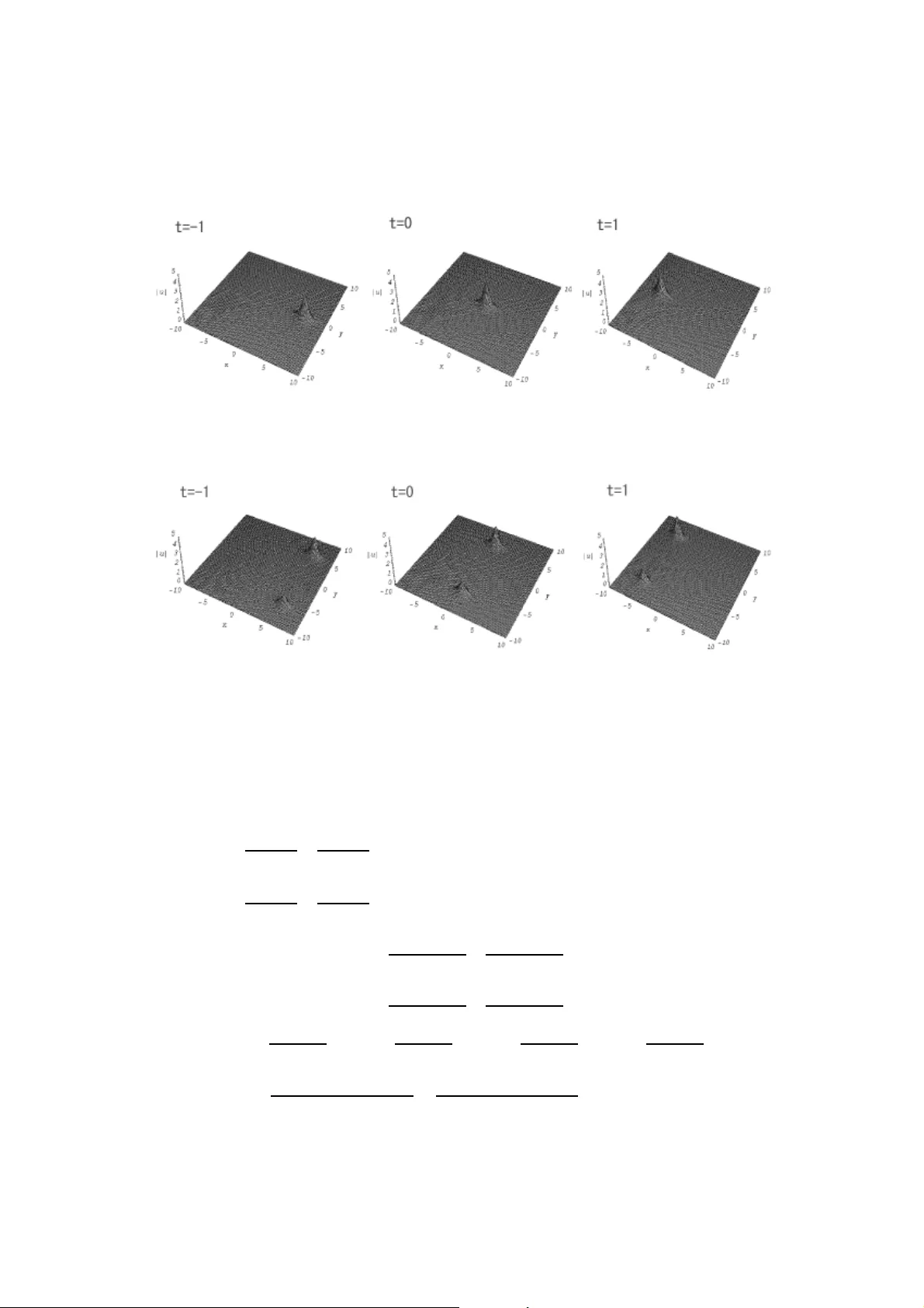
Localized Solitons of a (2+1)-dimensional Nonlocal Nonlinear Schr ¨ odinger Equation K en-ichi Maruno 1 † 1 Department of Mathematics, The Uni v ersity of T exas-P an American, Edinbur g, TX 78539-2999 Y asuhiro Ohta 2 2 Department of Mathematics, K o be Uni versity , Rokko, K obe 657-8 501, Japan October 31, 2018 Abstract An inte grable (2+1)-d imensional nonlocal non linear Schr ¨ oding er equa- tion is dis cussed. The N -solito n soluti on is g iv en by Gram type determinant . It is found that the localized N-soliton solution has interesting interac tion beha vior which shows change of amplitude of locali zed pulses after colli- sions. 1 Introduction The nonlinear Schr ¨ odinger (NLS) equation , i ψ t = ψ xx + α | ψ | 2 ψ , (1) is th e most im portant soliton equation which is a widely used m odel for i n vesti- gating the ev olution of puls es in optical fiber and of surface gra vity wa ves w ith 1 narro w-banded spectra in fluid [1]. The study of v ector and non local analog ues of the NLS equation has received cons iderable attention rece ntly from both physical and mathematical points of view [1, 2, 3, 4, 5, 6]. In this Letter , we dis cuss a (2+1)-dimensional nonlocal nonlin ear Schr ¨ odinger (2DNNLS) equation: i u t = u xx + 2 u Z ∞ − ∞ | u | 2 d y , (2) where u = u ( x , y , t ) is a compl ex function and x , y , t are real. The Gram type deter - minant solution is presented and localized soliton interactions are studied. 2 Determi nant Solu tion Using the dependent var iable transform ation u ( x , y , t ) = g ( x , y , t ) f ( x , t ) , u ∗ ( x , y , t ) = g ∗ ( x , y , t ) f ( x , t ) , where f is rea l and ∗ is complex con jugate, we ha ve bilinear equations [7] ( D 2 x − i D t ) g · f = 0 , (3) ( D 2 x + i D t ) g ∗ · f = 0 , (4) D 2 x f · f = 2 Z ∞ − ∞ gg ∗ d y . (5) These bilinear equations hav e the following Gram determi nant sol ution which is the N -soli ton solution of the 2DNNLS equation: f =      A N I N − I N B N      , g =         A N I N e T N − I N B N 0 T 0 − a N 0         , g ∗ = −         A N I N 0 T − I N B N a ∗ T N − e ∗ N 0 0         , where A N =       e ξ 1 + ξ ∗ 1 p 1 + p ∗ 1 e ξ 1 + ξ ∗ 2 p 1 + p ∗ 2 · · · e ξ 1 + ξ ∗ N p 1 + p ∗ N e ξ 2 + ξ ∗ 1 p 2 + p ∗ 1 e ξ 2 + ξ ∗ 2 p 2 + p ∗ 2 · · · e ξ 2 + ξ ∗ N p 2 + p ∗ N . . . . . . . . . . . . e ξ N + ξ ∗ 1 p N + p ∗ 1 e ξ N + ξ ∗ 2 p N + p ∗ 2 · · · e ξ N + ξ ∗ N p N + p ∗ N       , 2 B N =       R ∞ − ∞ a ∗ 1 a 1 d y p ∗ 1 + p 1 R ∞ − ∞ a ∗ 1 a 2 d y p ∗ 1 + p 2 · · · R ∞ − ∞ a ∗ 1 a N d y p ∗ 1 + p N R ∞ − ∞ a ∗ 2 a 1 d y p ∗ 2 + p 1 R ∞ − ∞ a ∗ 2 a 2 d y p ∗ 2 + p 2 · · · R ∞ − ∞ a ∗ 2 a N d y p ∗ 2 + p N . . . . . . . . . . . . R ∞ − ∞ a ∗ N a 1 d y p ∗ N + p 1 R ∞ − ∞ a ∗ N a 2 d y p ∗ N + p 2 · · · R ∞ − ∞ a ∗ N a N d y p ∗ N + p N       , and I N is the N × N identi ty matrix, a T is the transpose of a , a N = ( a 1 , a 2 , · · · , a N ) , e N = ( e ξ 1 , e ξ 2 , · · · , e ξ N ) , 0 = ( 0 , 0 , · · · , 0 ) , ξ i = p i x − i p 2 i t , ξ ∗ i = p ∗ i x + i p ∗ i 2 t , 1 ≤ i ≤ N , and p i is a complex wa ve number of i -th so liton and a i ≡ a i ( y ) i s a complex phase function of i -th solit on. Here, we show th at eq.(5) has the above Gram determinant soluti on. Let us denote the ( i , j ) -cofactor of the matrix M = A N I N − I N B N ! as ∆ i j . Then the x -deri vati ve of f = det M is given by f x = N ∑ i = 1 N ∑ j = 1 ∆ i j ∂ ∂ x e ξ i + ξ ∗ j p i + p ∗ j = N ∑ i = 1 N ∑ j = 1 ∆ i j e ξ i + ξ ∗ j =         A N I N e T N − I N B N 0 T − e ∗ N 0 0         . (6) In the Gram determinant expression of f , di viding i -th row by e ξ i and multiplying ( N + i ) -th colu mn b y e ξ i for i = 1 , · · · , N , and dividing j -th col umn by e ξ ∗ j and multiply ing ( N + j ) -th row by e ξ ∗ j for j = 1 , · · · , N , we obtain another determi nant expression of f , f = det M ′ , where M ′ = A ′ N I N − I N B ′ N ! , 3 A ′ N =      1 p 1 + p ∗ 1 · · · 1 p 1 + p ∗ N . . . . . . . . . 1 p N + p ∗ 1 · · · 1 p N + p ∗ N      , B ′ N =       e ξ ∗ 1 + ξ 1 R ∞ − ∞ a ∗ 1 a 1 d y p ∗ 1 + p 1 · · · e ξ ∗ 1 + ξ N R ∞ − ∞ a ∗ 1 a N d y p ∗ 1 + p N . . . . . . . . . e ξ ∗ N + ξ 1 R ∞ − ∞ a ∗ N a 1 d y p ∗ N + p 1 · · · e ξ ∗ N + ξ N R ∞ − ∞ a ∗ N a N d y p ∗ N + p N       . Thus the x -deri vati ve of f is also written as f x = N ∑ i = 1 N ∑ j = 1 ∆ ′ N + i , N + j ∂ ∂ x e ξ ∗ i + ξ j R ∞ − ∞ a ∗ i a j d y p ∗ i + p j = N ∑ i = 1 N ∑ j = 1 ∆ ′ N + i , N + j e ξ ∗ i + ξ j Z ∞ − ∞ a ∗ i a j d y = Z ∞ − ∞ N ∑ i = 1 N ∑ j = 1 ∆ ′ N + i , N + j e ξ ∗ i + ξ j a ∗ i a j d y where ∆ ′ i j is the ( i , j ) -cofactor of M ′ . Therefore we ha ve f x = Z ∞ − ∞       A ′ N I N 0 T − I N B ′ N ˜ a ∗ T N 0 − ˜ a N 0       d y = Z ∞ − ∞       A N I N 0 T − I N B N a ∗ T N 0 − a N 0       d y , where ˜ a N = ( e ξ 1 a 1 , · · · , e ξ N a N ) . By differentiating the abo ve f x by x , we get f xx = Z ∞ − ∞            A N I N e T N 0 T − I N B N 0 T a ∗ T N − e ∗ N 0 0 0 0 − a N 0 0            d y . 4 On the other hand, using the Jacobi formula for determinant[7], we hav e gg ∗ =      A N I N − I N B N      ×            A N I N e T N 0 T − I N B N 0 T a ∗ T N − e ∗ N 0 0 0 0 − a N 0 0            −         A N I N e T N − I N B N 0 T − e ∗ N 0 0         ×       A N I N 0 T − I N B N a ∗ T N 0 − a N 0       . Here we note th at the y -dependence in right-hand si de appears only in the l ast row and last column of the second determinant in each term. Thus we obtain Z ∞ − ∞ gg ∗ d y = f f xx − f x f x , which is a bilinear equation (5). Since eqs.(3) and (4) are bilinear equations for the NL S equation and do not include y , we can pro ve in the same way in the NLS equation that th e above Gram determinant sol ution satisfies the bilinear identit ies (3) and (4), i.e., we can show easily that the bil inear equations (3) and (4) are made from a pair of J acobi identities, respectively . 3 Localized Solitons Using the above form ula, we can make 1-soliton solution as follo ws: u = g f = a 1 e ξ 1 1 + R ∞ − ∞ a ∗ 1 a 1 d y ( p ∗ 1 + p 1 ) 2 e ξ 1 + ξ ∗ 1 , u ∗ = g ∗ f = a ∗ 1 e ξ ∗ 1 1 + R ∞ − ∞ a ∗ 1 a 1 d y ( p ∗ 1 + p 1 ) 2 e ξ 1 + ξ ∗ 1 , (7) where f =         e ξ 1 + ξ ∗ 1 p 1 + p ∗ 1 1 − 1 R ∞ − ∞ a ∗ 1 a 1 d y p ∗ 1 + p 1         = 1 + R ∞ − ∞ a ∗ 1 a 1 d y ( p ∗ 1 + p 1 ) 2 e ξ 1 + ξ ∗ 1 , 5 g =           e ξ 1 + ξ ∗ 1 p 1 + p ∗ 1 1 e ξ 1 − 1 R ∞ − ∞ a ∗ 1 a 1 d y p ∗ 1 + p 1 0 0 − a 1 0           = a 1 e ξ 1 , g ∗ = −           e ξ 1 + ξ ∗ 1 p 1 + p ∗ 1 1 0 − 1 R ∞ − ∞ a ∗ 1 a 1 d y p ∗ 1 + p 1 a ∗ 1 − e ξ ∗ 1 0 0           = a ∗ 1 e ξ ∗ 1 . If we choose a 1 ( y ) = α 1 sech ( k ( y + η 0 )) w here α 1 is a complex number and k and η 0 are real numbers, u = α 1 sech ( k ( y + η 0 )) e ξ 1 1 + ( 2 / k ) | α 1 | 2 ( p ∗ 1 + p 1 ) 2 e ξ 1 + ξ ∗ 1 = α 1 2 √ A sech ( ky + η 0 ) sech  ξ 1 + ξ ∗ 1 2 + 1 2 log A  e ξ 1 − ξ ∗ 1 2 , where A = ( 2 / k ) | α 1 | 2 ( p ∗ 1 + p 1 ) 2 . In this case, we ha ve a localized pulse as shown in figure 1. If we c hoose a 1 ( y ) = α 1 sech ( k ( y + η 1 )) + α 2 sech ( k ( y + η 2 )) where α 1 and α 2 are complex numbers and k , η 1 and η 2 are real numbers, u = ( α 1 sech ( k ( y + η 1 )) + α 2 sech ( k ( y + η 2 ))) e ξ 1 1 + ( 2 / k )( | α 1 | 2 + | α 2 | 2 )+ 4 ( η 1 − η 2 )( α 1 α ∗ 2 + α ∗ 1 α 2 ) / ( e k ( η 1 − η 2 ) − e − k ( η 1 − η 2 ) ) ( p ∗ 1 + p 1 ) 2 e ξ 1 + ξ ∗ 1 = 1 2 √ A ( α 1 sech ( k ( y + η 1 )) + α 2 sech ( k ( y + η 2 )) × sech  ξ 1 + ξ ∗ 1 2 + 1 2 log A  e ξ 1 − ξ ∗ 1 2 , where A = ( 2 / k )( | α 1 | 2 + | α 2 | 2 )+ 4 ( η 1 − η 2 )( α 1 α ∗ 2 + α ∗ 1 α 2 ) / ( e k ( η 1 − η 2 ) − e − k ( η 1 − η 2 ) ) ( p ∗ 1 + p 1 ) 2 . W e see two localized p ulses in figure 2. These two lo calized pulses t ra vel parallel to the x - axis. W ith a 1 ( y ) = ∑ M j α j sech ( k ( y + η j )) , we can see M -l ocalized pulses trav- elling parallel to the x -axis. W e call this M -localized pu lse the ( 1 , M ) -localized pulse solution. In the general case of puls e solu tions generated from the N -so liton formula, it is named by ( N , M ) -localized pulse sol ution. 6 Figure 1: 1-soliton solution. α 1 = 1 + 2 i , p 1 = 2 + 3 i , k = 3 , η 0 = 0 . Figure 2: 1-soliton solution . α 1 = 1 + 2 i , α 2 = 1 / 2 + i , p 1 = 2 + 3 i , k = 3 , η 1 = − 6 , η 2 = 6 . Next, we consi der t he case of N = 2, i.e. 2 -soliton sol ution. Using t he d eter - minant form of N -so liton solution, we ha ve f =                  e ξ 1 + ξ ∗ 1 p 1 + p ∗ 1 e ξ 1 + ξ ∗ 2 p 1 + p ∗ 2 1 0 e ξ 2 + ξ ∗ 1 p 2 + p ∗ 1 e ξ 2 + ξ ∗ 2 p 2 + p ∗ 2 0 1 − 1 0 R ∞ − ∞ a ∗ 1 a 1 d y p ∗ 1 + p 1 R ∞ − ∞ a ∗ 1 a 2 d y p ∗ 1 + p 2 0 − 1 R ∞ − ∞ a ∗ 2 a 1 d y p ∗ 2 + p 1 R ∞ − ∞ a ∗ 2 a 2 d y p ∗ 2 + p 2                  = 1 + c 11 p ∗ 1 + p 1 e ξ 1 + ξ ∗ 1 + c 12 p ∗ 1 + p 2 e ξ ∗ 1 + ξ 2 + c 21 p ∗ 2 + p 1 e ξ 1 + ξ ∗ 2 + c 22 p ∗ 2 + p 2 e ξ 2 + ξ ∗ 2 +  c 12 c 21 − c 11 c 22 ( p ∗ 2 + p 1 )( p ∗ 1 + p 2 ) + c 11 c 22 − c 12 c 21 ( p ∗ 1 + p 1 )( p ∗ 2 + p 2 )  e ξ 1 + ξ 2 + ξ ∗ 1 + ξ ∗ 2 , 7 g =                    e ξ 1 + ξ ∗ 1 p 1 + p ∗ 1 e ξ 1 + ξ ∗ 2 p 1 + p ∗ 2 1 0 e ξ 1 e ξ 2 + ξ ∗ 1 p 2 + p ∗ 1 e ξ 2 + ξ ∗ 2 p 2 + p ∗ 2 0 1 e ξ 2 − 1 0 R ∞ − ∞ a ∗ 1 a 1 d y p ∗ 1 + p 1 R ∞ − ∞ a ∗ 1 a 2 d y p ∗ 1 + p 2 0 0 − 1 R ∞ − ∞ a ∗ 2 a 1 d y p ∗ 2 + p 1 R ∞ − ∞ a ∗ 2 a 2 d y p ∗ 2 + p 2 0 0 0 − a 1 − a 2 0                    = a 1 e ξ 1 + a 2 e ξ 2 + ( c 12 a 1 − c 11 a 2 )( p 1 − p 2 ) ( p ∗ 1 + p 1 )( p ∗ 1 + p 2 ) e ξ 1 + ξ ∗ 1 + ξ 2 + ( c 22 a 1 − c 21 a 2 )( p 1 − p 2 ) ( p ∗ 2 + p 1 )( p ∗ 2 + p 2 ) e ξ 2 + ξ ∗ 2 + ξ 1 , g ∗ = −                     e ξ 1 + ξ ∗ 1 p 1 + p ∗ 1 e ξ 1 + ξ ∗ 2 p 1 + p ∗ 2 1 0 0 e ξ 2 + ξ ∗ 1 p 2 + p ∗ 1 e ξ 2 + ξ ∗ 2 p 2 + p ∗ 2 0 1 0 − 1 0 R ∞ − ∞ a ∗ 1 a 1 d y p ∗ 1 + p 1 R ∞ − ∞ a ∗ 1 a 2 d y p ∗ 1 + p 2 a ∗ 1 0 − 1 R ∞ − ∞ a ∗ 2 a 1 d y p ∗ 2 + p 1 R ∞ − ∞ a ∗ 2 a 2 d y p ∗ 2 + p 2 a ∗ 2 − e ξ ∗ 1 − e ξ ∗ 2 0 0 0                     = a ∗ 1 e ξ ∗ 1 + a ∗ 2 e ξ ∗ 2 + ( c 21 a ∗ 1 − c 11 a ∗ 2 )( p ∗ 1 − p ∗ 2 ) ( p ∗ 1 + p 1 )( p 1 + p ∗ 2 ) e ξ 1 + ξ ∗ 1 + ξ ∗ 2 + ( c 22 a ∗ 1 − c 12 a ∗ 2 )( p ∗ 1 − p ∗ 2 ) ( p 2 + p ∗ 1 )( p 2 + p ∗ 2 ) e ξ 2 + ξ ∗ 2 + ξ ∗ 1 , where c i j = R ∞ − ∞ a ∗ i a j d y / ( p ∗ i + p j ) . T o make four localized puls es, i.e. ( 2 , 2 ) -localized pulse solution, we consider a i ( y ) = ∑ 2 j = 1 α 2 ( i − 1 )+ j sech ( k ( y + η j )) . T hen c i j is giv en as follo ws. c i j = ( 2 / k )( α ∗ 2 ( i − 1 )+ 1 α 2 ( j − 1 )+ 1 + α ∗ 2 ( i − 1 )+ 2 α 2 ( j − 1 )+ 2 ) ( p ∗ i + p j ) + 4 ( η 1 − η 2 )( α 2 ( j − 1 )+ 1 α ∗ 2 ( i − 1 )+ 2 + α ∗ 2 ( i − 1 )+ 1 α 2 ( j − 1 )+ 2 ) ( e k ( η 1 − η 2 ) − e − k ( η 1 − η 2 ) )( p ∗ i + p j ) . Figure 3 is an example of ( 2 , 2 ) -localized pul se solution. It is observed that 4 localized pul ses suddenl y change the heig ht of pulses after a colli sion. Each pair 8 Figure 3 : (2,2)-lo calized pu lse sol ution. α 1 = 1 + i , α 2 = 1 , α 3 = 1 , α 4 = 1 , p 1 = 3 / 2 − 5 i / 2 , p 2 = 3 − i , k = 2 , η 1 = − 5 , η 2 = 5 . of pulses on lines parallel t o the x -axis colli des, then t he t otal mass of pulses is redistributed. In th e case of figure 3, t he h eight of a l ocalized pulse become very small after a coll ision. Although there is a distance between two pul ses on a li ne parallel to t he x -axis and oth er two pulses on anot her line, the col lision causes an ef fect of 4-pu lse interaction. As t his example, solutions of the 2DNNLS equation hav e very complicated and interesting properties. 4 Conclusio n W e h a ve discussed an integrable 2DNNLS equation and sho wn that the N -solito n solution o f t he 2DNNLS equation is gi ven by the Gram t ype determin ant and solutions can be localized in x - y plane. Note that the integrable 2DNNLS equ ation discussed in this Letter can be considered as the vec tor NLS equation with infinitely many components [8, 9, 10, 1]. This fact suggests that the vector soliton equations can produ ce nonlocal multi-dim ensional soliton e quation s ha ving localized pulses. It sho uld be noted that a model for second harmonic generation, i.e., quadratic solitons, w as di scussed in the p aper by Nikolov et al., and they discus sed the relationship between a nonlocal soliton equation and a vector sol iton s ystem [5]. Finding physi cal s ystems which could be described b y the 2 DNNLS equation is an interesting problem. Note a dded in proof: After the acceptance of this Letter for pu blication, the 9 authors noticed the 2DNNLS equation (2) is equiv alent t o eq.(7.86 ) in ref.[11]. Howe ver , as far as we know , the N-so liton solution has no t been obt ained so far . The autho rs th ank Dr . T akayuki Tsuchi da for l etting us know the paper by Za- kharov [11]. References [1] M. J. Ablowitz, B. Prinari and A. D. Trubatch, Discr ete and Continuous Nonlinear Schr ¨ odinger Systems (Cambridge Uni versity Press, 2004). [2] D. Pelinovsky , Phys. Lett. A 197 (1995) 401. [3] D. Pelinovsky and R. H. J. Grimshaw , J. Math. Phys. 36 (1995) 4203. [4] W . Kr ´ oli ko wski and O. Bang, Phys. Re v . E 63 (2000) 016610. [5] N. I. Nikolov , D. Neshev , W . Kr ´ o liko wski and O. Bang, Phys. Rev . E 68 (2003) 036614. [6] B. Deconinck and J. N. Kutz, Phys. Lett. A 319 (2003) 97. [7] R. Hirota, The Dir ect Meth od in Soliton T heory (Cambridge University Press, 2004). [8] S. V . Manakov , Sov . Phys. JETP 38 (1974) 248. [9] R. Radhakrishnan, M. Lakshmanan, and J. Hietarinta, Phys. Rev . E 56 (1997) 2213. [10] P . D. Mil ler , Phys. Lett. A 101 (1997) 17. [11] V . E. Zakharov , in Soli tons, ed. Bull ough and Caudrey , T opics in Current Physics (Springer , Berlin - New Y ork, 1980) 243. 10