Organization of modular networks

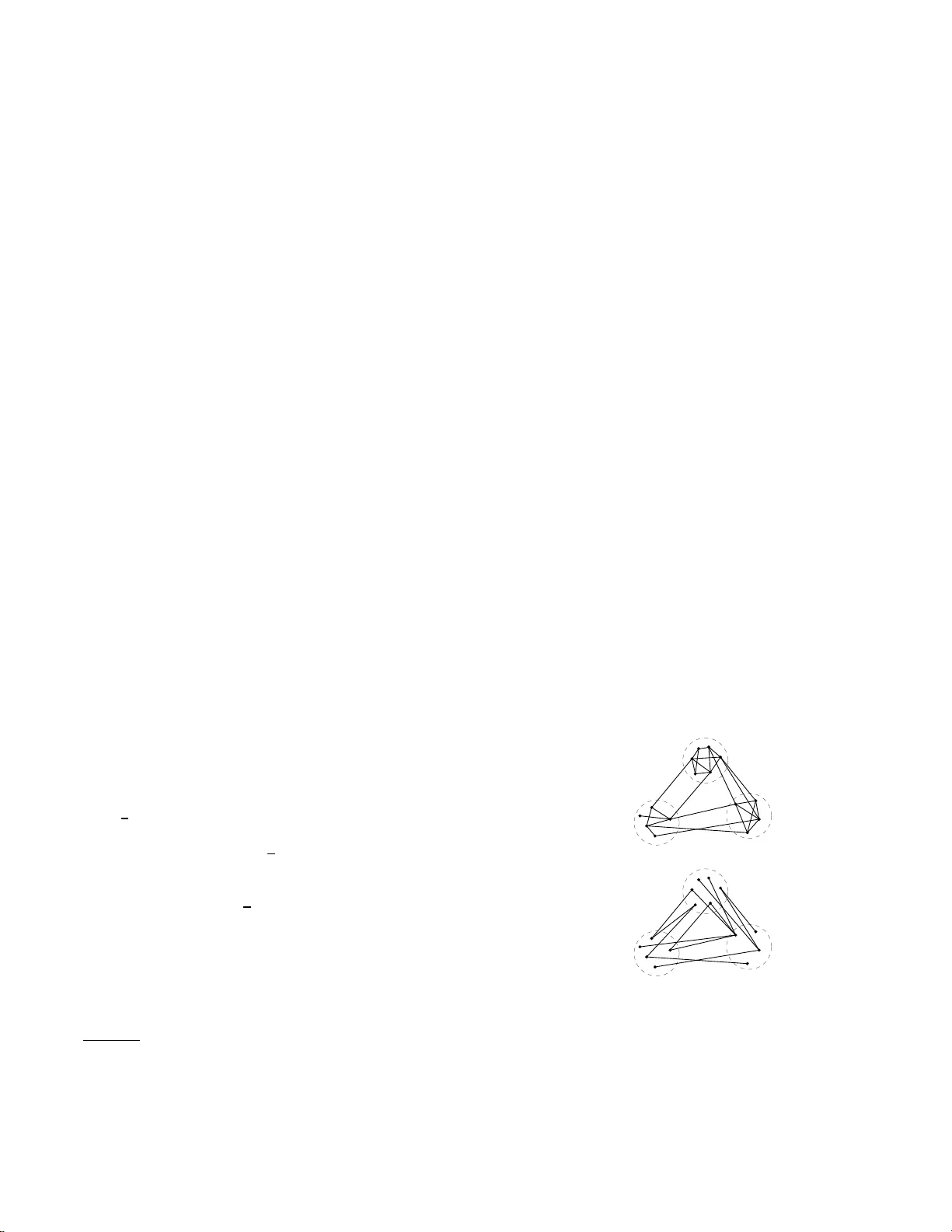
Organization of mo dular netw orks S. N. Dorogovtsev, 1, 2 , ∗ J. F. F. Mendes, 1 , † A. N. Samukhin, 1, 2 , ‡ and A. Y. Zyuzin 2 , § 1 Dep artamento de F ´ ısic a da Uni versidade de Aveir o, 3810-193 Aveir o, Portugal 2 A. F. Ioffe Physic o-T e chnic al Institute, 194021 St. Petersbur g, Rus sia W e examine the global organizati on of heterogeneous equilibrium netw orks consisting of a n umber of w ell distinguished interconnected parts—“communities” or modules. W e d evelop an analytical approac h allo wing us to obtain the statis tics of connected comp onen ts and an in terve rtex distance distribution in these mo dular netw orks, and to describ e their global organization and structu re. In p articular, w e stud y the evol ution of the interv ertex distance distribution with an increasing num b er of interlinks connecting tw o infi nitely large uncorrelated n etw orks. W e demonstrate that even a relatively small num b er of shortcuts u nite the netw orks into one. In more precise t erms, if the number of the interlinks is any finite fraction of the total number of connections, th en the interv ertex distance distribution approac hes a d elta-function p eaked form, and so the netw ork is united. P ACS nu mbers: 02.10.Ox, 89 .20.Hh, 89.75.Fb I. INTRO DUCTION Many real-world netw or k s con tain pr inc ipa lly distinct parts with d ifferent ar c hitectures. In this se nse, t hey are strongly hetero geneous. F or example, the In ternet—the net of physically in ter connected computers—is connected to mobile cellular netw o rks. One should note that the issue of the net work heterogeneity is a mo ng key pr ob- lems in the statistica l mechanics of complex netw ork s [1, 2 , 3, 4, 5, 6 , 7]. The ques tion is how do the net- work’s inhomo geneit y influence its global structure? The quantitativ e descr iption of the g lobal or ganization o f a net work is essentially based on the statistics of n -th com- po nen ts of a vertex in the netw o r k, par ticularly , on the statistics of their sizes [8, 9, 10]. The n -th comp onent o f a vertex is d efined as a set of vertices which a re not farther than distance n fro m a given vertex. F ro m this statis- tics, o ne c a n ea sily find less informative but very us e ful characteristics—the distribution of interv ertex distances and its first moment, the av erage interv ertex dista nc e . In the netw orks with the s ma ll-w orld pheno menon, so - called “small worlds”, the mean length of the shor test path ℓ ( N ) b et ween tw o vertices g r ows slow er tha n a n y po sitiv e p ow er o f the netw or k size N (the total num ber of vertices). Rather t ypically , ℓ ( N ) ∼ ln N . As a r ule , in in- finite small w orlds, a distribution of intervertex distances approaches a delta -function for m, where the mean width δ ℓ is muc h smaller tha n ℓ . Moreover, in uncorr e lated net- works, δ ℓ ( N → ∞ ) → const. So, in simple ter ms, ver- tices in these infinite net works are almost surely mutually equidistant. This statement can be easily understo o d if a net w ork has no weakly connec ted separ ate parts [11]. In this pap er we co nsider a co ntrasting situatio n. Our ∗ Electronic address: sdorogov@ua.pt † Electronic address: jf mendes@ua.pt ‡ Electronic address: samukhin@ua.pt § Electronic address: A. Zyuzin@mail.ioffe.ru net works are divided into a num ber of non-overlapping but interlinked subnetw orks, say j = 1 , 2 , . . . , m . What is imp ortant, we suppos e that the connections b etw een these subnetw ork s are orga nized differently than inside them, s e e Fig. 1. This assumption results in a global (or one may s a y , macrosco pic) heter ogeneity of a net- work. Using the p opular term “communit y ” , one can say that our netw or ks hav e well distinguished communities or mo dules. Mo dular ar c hitectures of this k ind lea d to a v ariety of effects [12, 1 3, 14, 15]. Figure 1 explains the difference betw een these mo dular netw or k s and the well studied m -partite netw orks [1 6, 17]. In this work we ana ly tically desc r ibe the statis tics of the n - th comp onents in these netw o rks when all m com- m unities are unco rrelated. F or the sake of brevity , here we consider only the case of m = 2, i.e., of tw o net- works with shortcuts b et ween them. As an immedia te (a) (b) FIG. 1: (a) An ex ample of a netw ork, which we study in this pap er in th e case m = 3. The structure of interconnections b et w een the th ree non- o verlapping subnetw orks differs from the structure of connections inside th ese subnetw orks. More- o ver, t he structures of the th ree subn et works may differ. (b) A contrasting ex ample of a 3-p artite graph, where conn ections b et w een vertice s of t h e same kind are absent. 2 l _ 2 l _ 1 0 P(l) 0 l l _ 2 l _ 1 l _ 1 l _ 2 l _ 1 (a) (b) (c) 0 P(l) 0 l + 0 P(l) 0 l FIG. 2: Schematic view of the evol ution of an interv ertex distance distribution with the grow ing number of shortcuts b et w een tw o large netw orks: (a) tw o separate n et w ork s; (b ) tw o netw orks with a single shortcut b etw een them; (c) tw o interco nnected netw orks, when the number of shortcuts is a finite fraction of the number of edges in the netw orks. ℓ 1 and ℓ 2 are the a verag e interv ertex distances in the first and in the second netw orks, respectively . application of this theory we find a distribution of inter- vertex distances. W e show how the global ar chitecture of this (la rge) netw or k evolv e s with an increasing num b er of s hortcuts, when tw o netw ork s merge into o ne. The question is: when is the mutual equidistance pr oper t y realised? How gener al is this feature? Figur e 2 s c hemat- ically pr esen ts our result. The conclus io n is that the equidistance is realize d when the num ber of s hortcuts is a finite fraction of the total num b er o f edges in the net- work. This finite frac tion may b e a rbitrary sma ll though bigger than 0. In this resp ect, the large netw o rk b ecomes united at ar bitr ary small co ncen trations of sho rtcuts. In Sec. I I we briefly pr e s en t our r esults. Sectio n I II describ es our general approach to these netw o rks based on the Z-transforma tio n (generating function) tec hnique. In Sec. IV we explain how to obtain the interv e rtex dis- tribution for the infinitely la rge net w orks. In Sec. V we discuss our r e s ults. Finally , for the sa k e of clarity , in the Appe ndix we outline the Z -transformation a pproach in applicatio n to the configura tion model of unco rrelated net works. II. MAIN RESUL TS W e apply the theory of Sec . II I to the following prob- lem. Two larg e uncorr elated netw or ks, of N 1 and N 2 vertices, hav e degree distributions Π 1 ( q ) and Π 2 ( q ) with conv er ging second moments. W e assume that de a d ends are a bsen t, i.e., Π 1 (1) = Π 2 (1) = 0, which guar an tees that finite co nnected comp onents are not es s en tial in the infinite netw ork limit (see Ref. [20 , 2 1]). L edges inter- connect ra ndomly chosen vertices of net 1 and randomly chosen vertices of net 2. F or simplicity , we assume in this problem that L is muc h sma ller than the total num ber of connections in the netw ork . The question is what is the form of the intervertex distance distributio n? In the infinite netw or k limit, to describ e this distribution, it is sufficiently to know three num ber s : an av erage distance ℓ 1 betw een vertices of subnetw o r k 1 , an av er age distance ℓ 2 betw een vertices of subnetw or k 2, and an av er age dis- tance d betw een a vertex fr o m subnetw ork 1 and a vertex from subnetw or k 2. These three num b ers give p ositions of the three pea ks in the distribution. Examining the v ariations of these three distances with L one can find when the equidistance pr o perty takes pla ce. W e intro duce the following quantities: K 1 , 2 ≡ X q,r q ( q − 1)Π 1 , 2 ( q , r ) / ¯ q 1 , 2 . (1) Here Π 1 , 2 ( q , r ) a re given distributions of vertices o f in tra- degree q and inter-degree r in subnet works 1 , 2 (see Sec. I II for more detail). ¯ q 1 and ¯ q 2 are mean interdegrees of vertices in subnetw o r ks 1 and 2 , resp ectively . In ter ms of K 1 and K 2 , the gener a lizations of the mean bra nching [ ζ in the standard configuration mo del, see Eqs. (A.13 ) in the App endix] are ζ 1 = K 1 + L 2 N 1 N 2 ¯ q 1 ¯ q 2 1 ( K 1 − K 2 ) K 2 1 , ζ 2 = K 2 − L 2 N 1 N 2 ¯ q 1 ¯ q 2 1 ( K 1 − K 2 ) K 2 2 . (2) Here we as sume that K 1 > K 2 and ζ 1 > ζ 2 . W e als o suppo se that ζ 1 , ζ 2 < ∞ . If the res ulting av erage distance ℓ 1 betw een v ertices o f subnetw o r k 1 is smaller than the corres p onding average distance ℓ 2 for subnet work 2, then we obtain asymptotically ℓ 1 ∼ = ln N 1 ln ζ 1 , (3) ℓ 2 ∼ = d + 1 ln ζ 2 ln  N 2 h ζ d 2 + C L i − 1  , (4) d ∼ = ℓ 1 + ln( N 2 / L ) ln ζ 2 . (5) Here the constant C is determined by the degree distribu- tions Π 1 ( q ) and Π 2 ( q ) and is indep e ndent of N 1 , N 2 , and L . In formula (4), ζ d 2 = ( N 1 N 2 / L ) ln ζ 2 / ln ζ 1 . Note that these as ymptotic estimates igno re constant a dditiv es. F ormulas (3)–(5) demonstra te that if L is a finite fractio n of the to ta l num b er of connections (in the infinite net- work limit), then ℓ 2 and d approach ℓ 1 . The differences 3 are o nly finite num b ers. Indeed, the second ter ms in re - lations (4) and (5) a re finite num b ers if N 2 / L → const. [When L is a finite frac tion o f the total num ber o f con- nections, ζ d 2 ≪ L in E q. (4).] On the other hand, when L is formally set to 1, r elation (5) gives d = ℓ 1 + ℓ 2 , see Fig. 2 (b). F urthermor e, a s suming L / N 1 , 2 → 0 as N 1 , 2 → ∞ , we have ℓ 2 ∼ = ln N 2 / ln ζ 2 according to rela- tion (4), since ζ d 2 = ( N 1 N 2 / L ) ln ζ 2 / ln ζ 1 ≫ L . W e a lso consider a sp e c ial situation where subnetw ork s 1 a nd 2 a re equa l, so K 1 = K 2 ≡ K , ¯ q 1 = ¯ q 2 , and N 1 = N 2 ≡ N . In this ca se the mean branching co e fficien ts are ζ 1 , 2 = K ± L N ¯ q 1 1 K . (6) With these ζ 1 and ζ 2 , the mean interv e r tex distances hav e the following a s ymptotics: ℓ 1 = ℓ 2 ∼ = ln N / ln ζ 1 and d ∼ = ℓ 1 + ln( N/ L ) / ln ζ 2 . F ormally setting L to 1 w e arrive at d = 2 ℓ 1 = 2 ℓ 2 . One sho uld stress that all the listed r esults indicate a s mooth cros so ver from t w o sep- arate netw or k s to a single united one: there is no sharp transition b et w een these tw o r egimes. II I. ST A TISTICS OF MODULAR NETWORKS W e co nsider tw o interlinked undirected netw o rks, o ne of N 1 , the o ther o f N 2 vertices. The adjacency matrix o f the joint netw ork, ˆ g , has the following str ucture: ˆ g =  ˆ g 1 ˆ h ˆ h T ˆ g 2  . Here ˆ g 1 = ˆ g T 1 and ˆ g 2 = ˆ g T 2 are N 1 × N 1 and N 2 × N 2 adjacency matrices of the fir st and of the seco nd subnet- works, r e spectively , and ˆ h is N 1 × N 2 matrix for in tercon- nections. W e use the following notations: la tin (greek) subscripts i , j , etc. ( α , β , etc.) ta k e v alues 1 , 2 , . . . , N 1 ( N 1 + 1 , N 1 + 2 , . . . N 1 + N 2 ). So, g j i , g β α , g j α and g β i are the matrix ele ments of ˆ g 1 , ˆ g 2 , ˆ h and ˆ h T , resp. W e assume the whole net work to b e a simple one, i.e., the matrix elemen ts o f ˆ g are either 0 or 1 , a nd the diagona l ones are all zero , g ii = g αα = 0. Every vertex in this netw or k has intra-degree and int er-degr e e. V ertex i b elonging to subnet w ork 1 has int ra-degr ee q i = P j g j i and int er-degr ee r i = P β g β i . V ertex α b elonging to subnet work 2 has intra-degr e e q α = P β g β α and inter-degree r α = P j g j α . The to - tal num b ers of intra- and interlinks are 2 L 1 = P j,i g ij , 2 L 2 = P β ,α g β α and L = P j,α g j α = P β ,i g β i . W e in tro duce a natural generaliza tio n of the c o nfigura- tion mo del (we recommend that a reader lo ok over Ap- pendix to recall the config uration mo del and the stan- dard analytical approach to the statistics of its com- po nen ts). In our random net work, intralinks in sub- net works 1 and 2 are uncor related, and the set of in- terlinks connecting them is als o uncorrelated. As in the config uration model, our statistical ensemble in- cludes all po ssible net works with given sequences of in tra- and inter-degrees for b oth subnetw orks. All the mem- ber s of the ensemble are taken with the same statisti- cal weigh t. Namely , there are N 1 , 2 ( N 1 , N 2 ; q , r ) vertices in s ubnet works 1 , 2 of intra-degree q and inter-degree r . Here P q,r N 1 , 2 ( N 1 , N 2 ; q , r ) = N 1 , 2 . The conditio n P q,r r N 1 ( N 1 , N 2 ; q , r ) = P q,r r N 2 ( N 1 , N 2 ; q , r ) = L , where L is the num b er of int erlinks, should b e ful- filled. W e a ssume that in the thermo dynamic limit N 1 → ∞ , N 2 → ∞ , N 2 / N 1 → κ < ∞ , we have N 1 , 2 ( N 1 , N 2 ; q , r ) / N 1 , 2 → Π 1 , 2 ( q , r ), wher e Π 1 and Π 2 are given distribution functions. Again, there is a condi- tion that the n um be r of edges fr om subnetw ork 1 to 2 is the same as from 2 to 1: ¯ r 1 ≡ ∞ X q,r =0 r Π 1 ( q , r ) = κ ∞ X q,r =0 r Π 2 ( q , r ) ≡ κ ¯ r 2 . (7) Here ¯ r 1 , 2 are av er age in ter-degrees of the vertices in sub- net works 1 and 2. The theory of uncorrelated netw or ks extensively use s the Z -representation (generating function) of a deg ree distribution: φ ( x ) = ∞ X q =0 Π ( q ) x q . (8) Here we introduce φ 1 , 2 ( x, y ) = ∞ X q,r =0 Π 1 , 2 ( q , r ) x q y r . (9) In Z-r e present ation, the av erage intra- ¯ q 1 and ¯ q 2 and int er- ¯ r 1 and ¯ r 2 degrees of subnetw orks 1 and 2, resp ec- tively , ar e ¯ q 1 , 2 = ∂ φ 1 , 2 ( x, y ) ∂ x     x = y =1 , ¯ r 1 , 2 = ∂ φ 1 , 2 ( x, y ) ∂ y     x = y =1 . (10) Let ( j, i ), ( β , α ) , ( j, α ) and ( β , i ) b e o rdered vertex pairs. Let us name their elements in the first and second po sition as final and initial, resp ectiv ely . An end vertex de gr e e distribution is the c o nditional probability for the final vertex of some (ra ndomly chosen) ordered pair of vertices to have intra- a nd interdegrees q and r , r espec- tively , provided the vertices in this pa ir are connected by an edge . W e hav e four distributio ns , each one dep ending 4 on t wo v aria bles: P 1 ( q , r ) = 1 2 L 1 X j i h g j i δ ( q j − 1 − q ) δ ( r j − r ) i , P 2 ( q , r ) = 1 2 L 2 X β ,α h g β α δ ( q β − 1 − q ) δ ( r β − r ) i , Q 1 ( q , r ) = 1 L X j,α h g j α δ ( q j − q ) δ ( r j − 1 − r ) i , Q 2 ( q , r ) = 1 L X β ,i h g β i δ ( q β − q ) δ ( r β − 1 − r ) i . (11) T aking into account definit ions of vertex degrees, we hav e P 1 , 2 ( q , r ) = ( q + 1 ) Π 1 , 2 ( q + 1 , r ) / ¯ q 1 , 2 , Q 1 , 2 ( q , r ) = ( r + 1) Π 1 , 2 ( q , r + 1) / ¯ r 1 , 2 . (12) In Z-repr esen tation these distribution functions take the following forms: ξ 1 ( x, y ) = 1 2 L 1 X j  q j x q j − 1 y r j  = 1 ¯ q 1 ∂ φ 1 ( x, y ) ∂ x , ξ 2 ( x, y ) = 1 2 L 2 X β  q β x q β − 1 y r β  = 1 ¯ q 2 ∂ φ 2 ( x, y ) ∂ x , η 1 ( x, y ) = 1 L X j  r j x q i y r j − 1  = 1 ¯ r 1 ∂ φ 1 ( x, y ) ∂ y , η 2 ( x, y ) = 1 L X β  r β x q β y r β − 1  = 1 ¯ r 2 ∂ φ 2 ( x, y ) ∂ y . (13) Let us in tro duce the n -th components o f ordered vertex pairs, C n,j i , C n,β α , C n,j α and C n,β i . These comp onents are sets, whose elements are vertices. As is natura l, the comp onen ts are empty , if the vertices in a pair ar e not connected. The firs t comp onen t is either one-element set consisting of the final vertex, o r empt y set. F o r example, C 1 ,β i is e ither vertex β or ∅ . The s econd comp onent , if nonempt y , contains also all the nearest neigh b o urs of the final vertex, except the initial one, and so o n. W e hav e four types of the comp onents of an edge: C n,j i , C n,β α , C n,j α and C n,β i . The y ar e defined in a recursive wa y similarly to the standard configura tio n mo del (see Appendix). Each of these four n -th comp onents itself consists of tw o disjoint sets: one of vertices in subnetw ork 1, the other—in subnetw or k 2. F o r example, C n,j i = C (1) n,j i ∪ C (2) n,j i . The s izes of the comp onent s ar e M (1) n,j i =    C (1) n,j i    , etc. T aking into acco unt the lo cally tree-like structure of o ur net work gives M (1 , 2) n,j i = g j i    1 0  + X k 6 = i M (1 , 2) n − 1 ,kj + X γ M (1 , 2) n − 1 ,γ j   , M (1 , 2) n,β α = g β a    0 1  + X k M (1 , 2) n − 1 ,kβ + X γ 6 = α M (1 , 2) n − 1 ,γ β   , M (1 , 2) n,j α = g j a    1 0  + X k M (1 , 2) n − 1 ,kj + X γ 6 = α M (1 , 2) n − 1 ,γ j x   , M (1 , 2) n,β i = g β i    0 1  + X k 6 = i M (1 , 2) n − 1 ,kβ + X γ M (1 , 2) n − 1 ,γ β   . (14) The co nfiguration mo del is uncorrelated random net- work. So all the ter ms on the r igh t-hand side of each of the four equations (14) are indep endent rando m v a r i- ables. Qua n tities within each o f tw o sums in these equa- tions are equa lly distributed. Their statistica l pr oper ties are also indep enden t of the deg ree dis tribution of the ini- tial vertex of the edge, i.e., of j o r β . The sizes of the connected comp onents of a n edge in different net works [e.g., M (1) n,j k and M (2) n,j k ] a re, g enerally , correla ted. So we intro duce four join t distribution func- tions of the comp onen t sizes in different netw or ks. In Z-repres en ta tion they are defined a s follows: ψ (1) n ( x, y ) = 1 2 L 1 * X j,i g j i x M (1) n,ji y M (2) n,ji + , ψ (2) n ( x, y ) = 1 2 L 2 * X β ,α g β α x M (1) n,β α y M (2) n,β α + , θ (1) n ( x, y ) = 1 L * X j,α g j α x M (1) n,jα y M (2) n,jα + , θ (2) n ( x, y ) = 1 L * X β ,i g β i x M (1) n,β i y M (2) n,β i + . (15) The recursive r elations for these distributions are straightforward gener alization of a relation for a usual uncorrela ted net work, without mo dularity [se e Eq. (A.7) in the App endix] ψ (1) n ( x, y ) = xξ 1 h ψ (1) n − 1 ( x, y ) , θ (2) n − 1 ( x, y ) i , ψ (2) n ( x, y ) = y ξ 2 h ψ (2) n − 1 ( x, y ) , θ (1) n − 1 ( x, y ) i , θ (1) n ( x, y ) = xη 1 h ψ (1) n − 1 ( x, y ) , θ (2) n − 1 ( x, y ) i , θ (2) n ( x, y ) = y η 2 h ψ (2) n − 1 ( x, y ) , θ (1) n − 1 ( x, y ) i . (16) 5 The n -th comp onent C n,i ( C n,α ) of vertex i ( α ) co n tains all vertices at distance n from vertex i ( α ) o r closer. Let M (1 , 2) n,i =    C (1 , 2) n,i    and M (1 , 2) n,α =    C (1 , 2) n,α    be siz e s of the comp onen ts [ C (1) and C (2) are the subset of C , co n taining vertices of the first a nd seco nd net works, resp ectively]. Using the lo cally tree-like structure of the netw ork and absence o f corr elations b e t ween its vertices, we obtain the Z- transform of the join t distributions of co mponent sizes: Ψ (1) n ( x, y ) = 1 N 1 * X i x M (1) n,i y M (2) n,i + = xφ 1 h ψ (1) n ( x, y ) , θ (1) n ( x, y ) i , Ψ (2) n ( x, y ) = 1 N 2 * X α x M (1) n,α y M (2) n,α + = y φ 2 h ψ (2) n ( x, y ) , θ (2) n ( x, y ) i . (17) The co nditional average sizes of the comp onents a re expressed in terms o f the deriv a tiv es of the corresp ond- ing distributio n functions a t the p oin t x = y = 1. F or example, the conditional average co mp onent sizes for an int ernal vertex pair in netw o rk 1 are ex pressed as follows: for the part, which b elongs to the fir st net work it is M (111) n = D g ij M (1) n,ij E / h g ij i = ∂ ψ (1) n ( x, y ) ∂ x      x = y =1 (18) for the comp onent part in netw o rk 1 , and M (211) n = D g ij M (2) n,ij E / h g ij i = ∂ ψ (1) n ( x, y ) ∂ y      x = y =1 (19) for the pa rt of the comp onen t, whic h is in netw or k 2. Here, (i) the first sup erscript index indicates whether the comp onen t is in subnetw ork 1 or 2, (ii) the second su- per script index indicates whether the fina l vertex is in subnetw ork 1 o r 2, and (iii) the thir d sup erscript index indicates whether the initia l vertex is in subnetw ork 1 or 2. F or the comp onents of a pair with initial vertex in net work 2 and final in netw ork 1 we hav e: M (112) n = D g iα M (1) n,iα E / h g iα i = ∂ θ (1) n ( x, y ) ∂ x      x = y =1 (20) and M (212) n = D g iα M (2) n,iα E / h g iα i = ∂ θ (1) n ( x, y ) ∂ y      x = y =1 , (21) and so on. Using Eqs. (16) one ca n der iv e recurrent rela tio ns for the av er age v alues of M n and M n − 1 . W e intro duce a pair of four-dimensional vectors: M (1) n =       M (111) n M (112) n M (121) n M (122) n       , M (2) n =       M (211) n M (212) n M (221) n M (222) n       . (22) Then the recur ren t relatio ns take the forms : M (1) n = b ζ M (1) n − 1 + m 1 , M (2) n = b ζ M (2) n − 1 + m 2 , (23) where b ζ =    ξ 11 0 ξ 21 0 η 11 0 η 21 0 0 η 22 0 η 12 0 ξ 22 0 ξ 12    , m 1 =    1 1 0 0    , m 2 =    0 0 1 1    . (24) Here ξ µν = ∂ µ ξ ν ( x, y ) | x = y =1 , η µν = ∂ µ η ν ( x, y ) | x = y =1 , µ, ν = 1 , 2 . The initial co nditions a re M (1) 1 = m 1 , M (2) 1 = m 2 . As for the av erage s izes of the n -th comp o- nent s of vertices, they ar e M (11) n = 1 N 1 * X i M (1) n,i + = ∂ Ψ (1) n ( x, y ) ∂ x      x = y =1 = 1 + ¯ q 1 M (111) n + ¯ r 1 M (112) n , M (21) n = 1 N 1 * X i M (2) n,i + = ∂ Ψ (1) n ( x, y ) ∂ y      x = y =1 = ¯ q 1 M (211) n + ¯ r 1 M (212) n , M (12) n = 1 N 1 * X α M (1) n,i + = ∂ Ψ (2) n ( x, y ) ∂ x      x = y =1 = ¯ q 2 M (122) n + ¯ r 2 M (121) n , M (22) n = 1 N 2 * X i M (2) n,i + = ∂ Ψ (2) n ( x, y ) ∂ y      x = y =1 = 1 + ¯ q 2 M (222) n + ¯ r 2 M (221) n . (25) Here, (i) the fir s t sup erscript index of M n indicates whether the comp onent is in subnetw ork 1 o r 2 , and (ii) the second sup erscr ipt index indicates whether a mother vertex is in subnetw o rk 1 or 2 . Recall that ¯ q 1 and ¯ q 2 are the mean num ber s of internal connections of vertices in subnetw ork s 1 a nd 2, resp ectively; ¯ r 1 is a mean num b er of connections of a vertex in s ubnet work 1, whic h go to subnetw ork 2; a nd finally ¯ r 2 is a mea n num b er of connec- tions of a vertex in subnetw o rk 2, which go to subnetw o rk 6 1. Relations (23) a nd (25) a llo w us to o bta in the av erage sizes of all comp onents. Example .—Since formulas in this s ection are r ather cum b e rsome, to help the readers, we pr esen t a simple demonstrative example of the a pplication o f these re- lations. Let us describ e the emer gence of a giant co n- nected comp onents in a symmetric situation, wher e both subnetw ork s hav e equal sizes and identical degree dis- tributions Π 1 , 2 ( q , r ) ≡ Π( q , r ). In this case , ξ 1 ( x, y ) = ξ 2 ( x, y ) ≡ ξ ( x, y ) and η 1 ( x, y ) = η 2 ( x, y ) ≡ η ( x, y ). Also, ψ (1) ( x, y ) = ψ (2) ( x, y ) ≡ ψ ( x, y ) and θ (1) ( x, y ) = θ (2) ( x, y ) ≡ θ ( x, y ). So the relative size S o f a gia n t con- nected comp onent takes the for m: S = 1 − φ ( t, u ) , (26) where t ≡ ψ (1 , 1) and u ≡ θ (1 , 1) a re non-trivial solutions of the equatio ns: t = ξ ( t, u ) , u = η ( t, u ) . (27) F or example, let the subnetw orks b e classic a l random graphs, and each vertex has no interlinks with a pr obabil- it y 1 − p and has a single interlink with the complimentary probability p . That is, Π( q , r ) = e − ¯ q ¯ q q q ! [(1 − p ) δ q, 0 + pδ q, 1 ] , (2 8) where ¯ q is the mean vertex intra-degree, s o φ ( x, y ) = e ¯ q ( x − 1) [1 − p + py ]. F or a single classica l r andom gra ph with vertices of av er age degre e ¯ q , Eqs. (A.15) and (A.17) g iv e the point of the birth of a gia n t connected co mponent, ¯ q = q c = 1, and the rela tiv e s ize of this comp onent S ∼ = 2( ¯ q − 1) in the critical reg ion. Let us now find the birth p oint ¯ q = q c ( p ) and the critical dependence S ( ¯ q , p ) in the mo dular netw or k. F or this netw o rk, we find ξ ( x, y ) = ∂ x φ ( x, y ) / ¯ q = φ ( x, y ) and η ( x, y ) = ∂ y φ ( x, y ) / ¯ r = e ¯ q ( x − 1) . Substituting these functions into E qs. (26) and (27) directly leads to the result: q c = 1 1 + p , S ∼ = 2 (1 + p ) 3 1 + 3 p  ¯ q − 1 1 + p  , (29) compare with a sing le clas s ical rando m gr aph. IV. INTER VER TEX D IST ANCE DISTRIBUTION As was explained in Sec. I I, the interv ertex distance distribution in the thermo dynamic limit is completely determined b y the three mean in tervertex distances: ℓ 1 for subnetw or k 1 , ℓ 2 for subnetw or k 2 , a nd d for pair s of vertices wher e the first vertex is in subnetw o r k 1 and the second is in subnetw ork 2. The idea o f the computa- tion of these intervertex distances is very similar to that in the standard configuratio n mo del, see the App endix, Eq. (A.18). How ever, the straightforw ard calculations for t wo interconnected netw orks are cumbers ome, so here we only indicate some p oints in our deriv ations without g o- ing int o technical details . The calculations are based on the so lution of r ecursive relations (23). As is usual, these relations should b e in- vestigated in the range 1 − x ≪ 1 , 1 − y ≪ 1 of the Z-transfor mation parameters. F o rtunately , the proble m can b e es s en tially reduced to the calcula tion of tw o high- est eigenv a lues o f a sing le 4 × 4 matrix. The r esulting eigenv a lues ζ 1 and ζ 2 for netw or ks with L / N 1 , 2 ≪ 1 ar e given by formulas (2) and (6). The n -th c omponent sizes are expres sed in terms of these eigenv alues. The lea d- ing co ntributions to the n -th c o mponent sizes turn out to b e linear combinations of powers of the mean branch- ings: Aζ n 1 + B ζ n 2 . T he factor s A and B do not dep end o n n . F or exa mple, when ζ 1 > ζ 2 , the main contributions to M (11) n and M (21) n lo ok a s ζ n 1 + [ L 2 / ( N 1 N 2 )] ζ n 2 and ( L / N 1 ) ζ n 2 , resp ectively . Here we omitted non-ess en tial factors and assumed a la rge n . This a pproximation is based on the tree a nsatz, that is on the loc ally tree- lik e structure of the netw o rk. This ansa tz works when the n - th comp onen ts a re muc h smaller than subnetw o r ks 1 and 2. So the in tervertex distances are obtained by compar- ing the sizes of re lev an t n -th comp onents of vertices with N 1 and N 2 . Since netw or ks 1 and 2 a re uncor related, this estimate g iv es only a co nstan t additive erro r which is muc h smaller than the main co ntribution of the order of ln N 1 , 2 . (See Ref. [10] fo r co mplicated ca lculations b e- yond the tree ansatz in the standard config ur ation mo del, which allow one to obtain this constant num b er.) One should emphasiz e an a dditional difficulty sp ecific for the netw or k s under consideration. The pr oblem is that in s ome r a nge o f N 1 and N 2 , and ζ 1 and ζ 2 , while an n -th compo nen t in, s a y , netw ork 1 is already o f size ∼ N 1 (failing tree ansatz), the corresp onding n -th comp onent in netw ork 2 is still muc h sma ller than N 2 . In ter ms of Sec. I II, this, e.g ., means that there exis ts a range of n , ℓ 1 1 , C n,ij is defined r ecursively as follows. If g j i = 0, all C n,j i = ∅ . Other wise, in C 2 ,ij there are also q j − 1 o ther v ertices, connected to the vertex j , the third comp o nen t C 3 ,ij contains a lso all other vertices, connected with ones of the second compo nen t, and so on, see Fig. 3. In the thermo dynamic limit ( N → ∞ ) almost every finite n - th comp onent of uncorr e la ted r andom gr aph is a tree. Then for the sizes (num b ers of vertices) of the comp onen ts, M n,ij = | C n,ij | we ha ve (assuming g j i = 1): M n,j i = 1 + X k 6 = i M n − 1 ,kj , (A.4) 8 with the initial condition M 1 ,j i = 1. Due to the ab- sence of corre la tions in the config ur ation mo del, M n,kj and M n,lj , k 6 = l , are indep e nden t equally distributed random v ar iables. W e define the distribution function of the n -th comp onent of an edge a s p n ( M ) = 1 2 L N X j,i =1 h g j i δ ( M n,ij − M ) i = N ( N − 1) 2 L h g j i δ ( M n,j i − M ) i = 1 h g j i i h g j i δ ( M n,j i − M ) i . (A.5) It is more conv enie nt to use the Z-transfor mation of this distribution: ψ n ( x ) = 1 2 L * N X i,j =1 g ij x M n,ij + = 1 h g ij i  g ij x M n,ij  . (A.6) Substituting E q. (A.4) int o Eq. (A.6) and using Eq. (A.3) gives ψ n ( x ) = x 2 L * N X j,i =1 g j i Y k 6 = i, 1 h g kj i  g kj x M n − 1 ,kj  + = x 2 L * N X j =1 q j [ ψ n − 1 ( x )] q j − 1 + = x e φ [ ψ n − 1 ( x )] . (A.7) Let C n,i be the n -th comp onen t of v ertex v i . This com- po nen t includes all vertices at distance n or c loser from vertex v i . (The 0-th comp onent of a vertex is empty .) Due to the absence of lo ops (tree-like structure) we hav e the following relatio n for the size of n -th co mponent of vertex v i , M n,i = |C n,i | , M n,i = 1 + X j M n − 1 ,ij . (A.8) So the n -th comp onent size distribution P n ( M ) = 1 N * N X i =1 δ ( M n,i − M ) + (A.9) is expressed in Z- representation as Ψ n ( x ) = 1 N * N X i =1 x M n,i + = xφ [ ψ n − 1 ( x )] . (A.10) The average s izes of subsequent n -th comp onents are related through the following eq ua tions: M n = Ψ ′ n (1) = 1 + ¯ q M n − 1 , (A.11) M n = 1 + ζ M n − 1 , (A.12) where ζ ≡ e φ ′ (1) = φ ′′ (1) ¯ q = 1 ¯ q ∞ X q =0 q ( q − 1)Π ( q ) = h q 2 i ¯ q − 1 , (A.13) which is the mean branching. If ζ < 1, b oth M n and M n hav e finite limits as n → ∞ . That is, the netw ork has no giant co nnected comp onent. If ζ > 1, a g ian t connected comp onen t ex is ts. Assuming ψ n = ψ n − 1 ≡ ψ in E q . (A.7), we obta in an equation for the dis tribution function of the sizes of edge’s connected comp onents, ψ ( x ) = x e φ [ ψ ( x )] , (A.14) which implicitly defines ψ ( x ). I f ζ > 1 , this equatio n has t wo solutions at x = 1. One is ψ (1) = 1, the other is some ψ (1) ≡ t < 1, t = e φ ( t ) . (A.15) F or any v alue of ζ , ψ n (1) = 1 . On the o ther hand, if ζ > 1, lim x → 1 − 0 lim n →∞ ψ n ( x ) = t < 1 . This is the probability that the connected c o mponent of a randomly chosen edge is finite. Then the probability that randomly chosen vertex b elongs to a finite co nnected compo nen t o f the graph is ∞ X q =0 Π ( q ) t q = φ ( t ) . (A.16) Therefore the num ber of vertices in the giant connected comp onen t in the thermo dynamical limit is M ∞ = N [1 − φ ( t )] . (A.17) One may find an intervertex distance distributio n from the mean sizes of the n -th comp onen ts of a vertex, see Ref. [8, 26]. The dia meter ℓ of the giant connected com- po nen t, i.e., the distance b et ween t wo randomly chosen vertices, is obtained from the relatio n ζ ∼ M ∞ ∼ N . So, if the s econd moment of the degre e distribution is finite, ℓ ∼ = ln aN ln ζ , (A.18) where a is some num ber of the order of 1. F or more straightforward calculations, see Refs. [10, 27]. [1] R. Alb ert and A.-L. Barab´ as i, Statistical mechanics of complex netw orks, Rev. Mod . Phys. 74 , 47 (2002). [2] S. N. Dorogo vtsev and J. F. F. Mendes, Evolution of 9 netw orks, Adv. Phys. 51 , 1079 (2002); Evolution of Net- works: F r om Biolo gic al Nets to the Internet and WWW (Oxford Universit y Press, Oxford, 2002). [3] M. E. J. Newman, The structure and function of complex netw orks, SI AM Rev iew 45 , 167 (2003). [4] R. P astor-Satorras and A. V espignani, Evolution and Structur e of the I ntern et: A Statistic al Physics Appr o ach (Cam bridge Universit y Press, Cambridge, 2004). [5] S. Boccaletti, V. Latora, Y . Moreno, M. Chav ez, and D.- U. Hwang, Complex Netw orks: S tructure and Dy namics, Phys. Rep orts 424 , 175 (2006). [6] G. Caldarelli, Sc ale-F r e e Networks (Oxford Universit y Press, Oxford, 2007). [7] S. N. D orogo vtsev, A. V. Goltsev, and J . F. F. Mendes, Critical ph enomena in complex netw orks, arXiv:0705.00 10 [cond-mat]. [8] M. E. J. Newman, S. H. Strogatz, and D . J. W atts, Ran- dom graphs with arbitrary d egree distribut ions and their applications, Phys. Rev. E 64 , 026118 (2001). [9] M. E. J. Newman, Random graphs as mo dels of netw orks, in H andb o ok of Gr aphs and Networks: F r om the Genome to the Internet , eds. S. Bornholdt and H. G. Sch uster (Wiley-VCH, Berlin, 2002), p. 35. [10] S. N. Dorogo vtsev, J. F. F. Mend es, and A. N . S am u khin, Metric structure of random net w orks, Nu cl. Ph ys. B 653 , 307 (2003). [11] One can easily u nderstoo d the vertex equidistance in typical infin ite small worlds in the follow ing wa y . The mean number of ℓ - t h nearest neighb ors of a vertex in small w orlds usually grows with ℓ as ζ , where ζ is the mean branching co efficien t , and ℓ . ℓ ( N ). This leads to the follo wing estimate for th e interve rtex distance distribution: P ( ℓ, N ) ∝ ζ θ ( ℓ ( N ) − ℓ ). In addition, one must tak e into accoun t normalization, whic h readil y giv es P ( ℓ, N ) → δ ( ℓ − ℓ ( N )) as N → ∞ . [12] P . P ollner, G. Palla, and T. Vicsek, Preferen t ial attach- ment of communities: the same principle, bu t a higher leve l, Europhys. Lett. 73 , 478 (2006). [13] K. Su c hec ki and J. A. H olyst, First order phase tran- sition in I sing mo del on t w o connected Barab´ asi-Alb ert netw orks, [14] R. K. P an and S. Sinha, Mo dular netw orks emerge from multiconstrain t optimization, Phys. Rev. E 76 , 045103 (R) (2007 ); The small w orld of modu lar net works, arXiv:0802.36 71 . [15] A. Galst yan and P . Cohen, Cascading dy namics in mo d- ular netw orks, Phys. Rev. E 75 , 036109 (2007). [16] M. E. J. Newman and J. Pa rk, Why social netw ork s are different from other types of netw orks, Phys. Rev . E 68 , 036122 (2003). [17] J.-L. Guillaume an d M. Latapy , Bipartite structu re of all complex netw orks, In formatio n Processing Letters 90 , 215 (2004). [18] B. Bollob´ as, Eur. J. Comb. 1 , 311 (1980). [19] E. A. Bender and E. R . Canfield, J. Com b in. Theory A , 24 , 296 (1978). [20] M. Mollo y an d B. Reed, Random Structu res and Algo- rithms 6 , 161 (1995). [21] M. Mollo y and B. Reed, Combinatorics, Probabilit y and Computing 7 , 295 (1998). [22] D. F ernh olz and V. Ramachandran, Cores and connec- tivity in sp arse random graph s, UTCS T echnical Rep ort TR04-13, 2004. [23] S. N. Dorogovtsev, A. V . Goltsev, and J . F. F. Mendes, k - core organization of complex netw orks, Phys. Rev . Let t . 96 , 040601 (2006); k -core architecture and k -core p erco- lation on complex netw ork s, Physica D 224 , 7 (2006); A. V. Goltsev, S. N. Dorogo v tsev, J. F. F. Mendes, k - core (b ootstrap) p ercolation on complex netw orks: Crit- ical phenomena and nonlo cal effects, Phys. Rev. E 73 , 056101 (2006). [24] J.I. Alva rez-Hamelin, L. D all´Asta, A . Barrat, and A. V espignani, k -core decomp osition: a to ol for the vi- sualization of large scale netw orks, Adv. Neural I n forma- tion Pro cessing Sy stems Canada 18 , 41 (2006). [25] S. Carmi, S. Havlin, S. Kirkp atric k , Y. Shavitt, and E. Shir, New mod el of Internet top olog y using k -shell decomp ositio n, PNAS 104 , 11150 (2007). [26] R. Cohen and S. Havli n, Scale-free netw orks are ultra- small, Phys. R ev. Lett. 90 , 058701 (2003). [27] A. F ronczak, P . F ronczak, and J. A. Holyst, Average path length in uncorrelated random netw orks with hid - den va riables, Phys. Rev. E 70 , 056110 (2004).