Approximation Algorithms for Bregman Co-clustering and Tensor Clustering

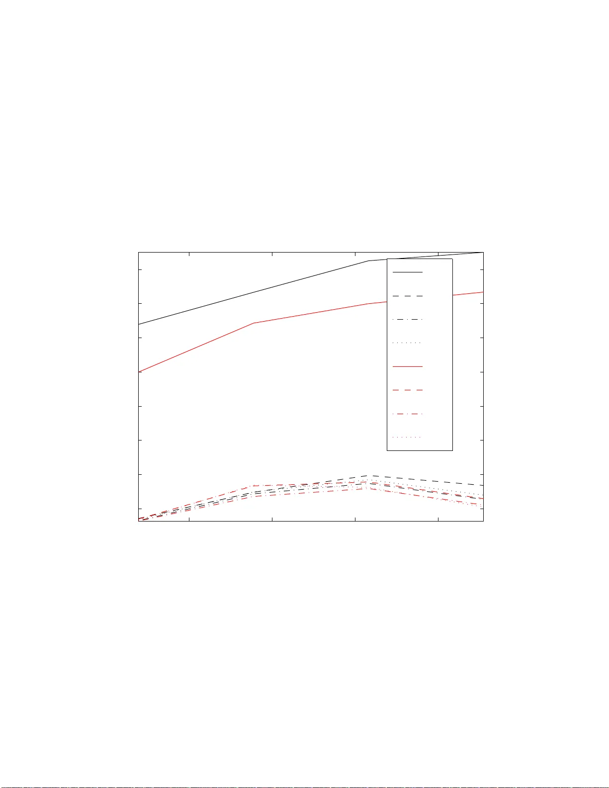
Appro ximatio n Algorithms for Bregma n Co-clusteri ng and T ensor Clusteri ng ∗ Stefanie Jegelk a MPI for Biological Cyb ernetics 72070 T ¨ ubingen, German y Suvrit Sra MPI for Biological Cyb ernetics 72070 T ¨ ubingen, German y Arindam Banerjee Univ. of Minnesota MN 55455, USA Abstract In the past few years pow erful generalizations to the Euclidean k-means p roblem hav e b een made, suc h as Bregman clustering [7], co-clustering (i.e., simultaneous clustering of ro ws and columns of an inpu t matrix) [9, 18], and tensor clustering [8, 34]. Like k-means, these more general problems also suffer from the NP-hardness of the associated optimization. Researc h ers hav e d evelo p ed appro x imation algorithms of v arying degrees of soph istication for k -means, k- medians, and more recently also fo r Bregman clustering [2]. How ever, there seem to b e no approximatio n algorithms for Bregman co- and tensor clustering. In this paper w e d erive the first (to our knowledge) guaran teed m eth od s for these increasingly imp ortant clustering settings. Going b eyond Bregman divergences, we also p ro ve an app ro x imation factor for tensor clustering with arbitrary separable metrics. Through extensive exp erimen ts we ev aluate the characteris t ics of our meth od , and show that it also has practical impact. 1 In tro d uction Partitioning data p o int s into clus ters is a fundamen tally hard problem. The well-kno wn Euclidean k- means pro blem that par titions the input data p oints (vectors in R d ) into K clusters while minimizing sums of their squared distances to corresp onding cluster centroids, is an NP har d problem [19] (exp o nential in d ). How ever, simple a nd frequently used pro cedures that ra pidly obtain lo cal minima exist since a long time [23, 28]. Because o f its wide applicability and impo rtance, the Euclidean k-means pr oblem has b een generalized in several directio ns. Specific ex amples relev ant to this pap er include: • Br e gman clustering [7], wher e instead of minimizing squar ed Euclidean distances one minimizes Bregman divergences (which ar e gene r alized distance functions, see (3.10) or [13] for details), • Br e gman c o-clustering [9 ] (which includes bo th Euclidean [16] and informa tion-theoretic c o- clustering [18] as s p ecia l ca ses), wher e the set of input vectors is viewed as a matrix and one simultane ously clusters r ows and columns to obtain coherent submatrices (co-clusters), while minimizing a Bregman divergence, and • T ensor clustering o r m ultiway clustering [34], esp ecia lly the version based on Breg man diver- gences [8], where one simu ltaneously clusters along v arious dimensions of the input tensor. F or these pro blems to o, the commonly use d heuristics p erform well, but do not provide theoretical guarantees (or at b est assur e lo cal optimality). F o r k-mea ns type clustering problems—i.e., pr oblems ∗ A part of the theory of this pap er appeared in MPI-TR-#177 [ 35]. 1 1.1 Contributions 2 BACK GROUND that gr oup together input vectors into clusters while minimizing “dista nce” to clus ter c e nt r oids— there exist several alg orithms that approximate a globally o ptimal solution. W e refer the reader to [1, 2, 6, 27], and the numerous references there in for more details. In stark co nt r ast, approximation algorithms for tenso r clustering are muc h less studied. W e are aware of only tw o very recent attempts (both papers are from 2008) for the tw o -dimensional sp ecial case of co-clustering , namely , [4] a nd [31]—and b oth of the pap ers follow similar approa ches to obtain their approximation guarantees. Both prov e a 2 α 1 -approximation for E uc lide a n c o -clustering, Puolam¨ aki et al. [31] a n additio na l factor o f (1 + √ 2) for binary matrices and a n ℓ 1 norm o b jective, and Anag nostop oulos et al. [4] a factor of 3 α 1 for co-clus tering rea l matric es with ℓ p norms. In all factors α 1 is an approximation guarantee for clustering either rows or co lumns. In this pap er, we build upo n [4] and o bta in approximation a lgorithms for tensor clustering with Br egman divergences and arbitrary separable metrics s uch as ℓ p -norms. The latter result is o f particular in ter est for ℓ 1 - norm based tens o r clustering, which may b e viewed a s a gener alization of k-media ns to tensor s . In the terminology of [7], we fo cus on the “blo ck a verage ” versions of co- and tensor clustering. Additional discussion a nd relev ant r eferences for co -clustering can b e found in [9], while for the lesser known problem of tensor cluster ing more ba ckground can be gained by refer ring to [3, 8, 10, 21, 29, 34]. 1.1 Con tributions The main contribution of this pap er is the analysis of an approximation alg orithm for tensor c lus ter- ing that achiev e s an appr oximation ra tio of O ( mα ), wher e m is the order of the tensor and α is the approximation factor of a corresp o nding 1 D clustering algorithm. O ur results apply to a fairly broad class of ob jective functions, including metric s such as ℓ p norms or Hilber tian metrics [2 4, 33], and divergence functions suc h a s Bregman divergences [13] (with some assumptions ). As corollaries , o ur results so lve tw o open problems p osed by [4], viz., whether their methods for Euclidean co-clustering could b e extended to Br egman co - clustering, a nd if one co uld extend the approximation guarantees to tensor clustering. Owing to the structure of the algo rithm, our results also give insight in to proprties of the tensor clustering problem as such, namely , a b ound on the amount of information inherent in the joint co nsideration of several dimensions. In addition, we provide ex tensive exp e rimental v alida tion of the theo retical claims, which for ms an additional contribution of this pap er . 2 Bac kground T raditionally , “center” bas ed cluster ing a lg orithms seek partitions o f columns o f an input matrix X = [ x 1 , . . . , x n ] into cluster s C = {C 1 , . . . , C K } , and find “centers” µ k that minimize the ob jective J ( C ) = X K k =1 X x ∈C k d ( x , µ k ) , (2.1) where the function d ( x , y ) measur es cluster quality . The “ce nter” µ k of cluster C k is given by the mean of the p o ints in C k when d ( x , y ) is a Bregman div er gence [7]. Co-clustering e xtends (2.1) to seek simultaneous partitions (and cen ters µ I J ) of rows and columns of X , so tha t the ob jective function J ( C ) = X I ,J X i ∈ I ,j ∈ J d ( x ij , µ I J ) , (2.2) is minimized; µ I J denotes the (sca lar) “center” of the cluster des crib ed by the row and column index sets, viz ., I and J . F ormulation (2.2) is eas ily genera lized to tensors, a s shown in Section 2.2 below. How ever, we fir st recall basic notation abo ut tenso r s b efore formally presenting the tensor clustering problem. T enso rs ar e well-studied in multilinear alge br a [22], and they ar e gaining imp o rtance in bo th data mining and machine learning applica tions [26, 36]. 2 2.1 T ensors 2 BACK GROUND 2.1 T ensors A lar ge part of the mater ial in this section is derived fro m the well-written pap e r o f de Silv a a nd Lim [17]—their notatio n turns out to b e particular ly suitable for our ana lysis. An or der- m tensor A may b e viewed as an element of the v ector s pace R n 1 × ... × n m (in this pap er we denote ma trices and tenso rs using sans- serif letters). An individual component o f the tensor A is represented b y the m ultiply- indexed v alue a i 1 i 2 ...i m , where i j ∈ { 1 , . . . , n j } for 1 ≤ j ≤ m . Multili near m atrix multiplication F or us the mos t impo rtant oper ation on tensors is that of m ultilinea r ma trix multiplication, which is a generalization of the familiar concept of matrix m ultiplica tio n. Matrices act on other matrice s by either left or rig ht m ultiplication. F or an or der-3 tensor , there are three dimensions on which a matrix ma y act via matrix multiplication. F or example, for an o r der-3 tensor A ∈ R n 1 × n 2 × n 3 , and three ma trices P ∈ R p 1 × n 1 , Q ∈ R p 2 × n 2 , and R ∈ R p 3 × n 3 , multiline ar matrix m ultiplic ation is the op eration defined by the action of these three matrices on the different dimensions of A tha t yields the tensor A ′ ∈ R p 1 × p 2 × p 3 . F ormally , the en tries of the tens o r A ′ are given by a ′ lmn = X n 1 ,n 2 ,n 3 i,j,k =1 p li q mj r nk a ij k , (2.3) and this op eration is written compactly as A ′ =  P , Q , R  · A . (2.4) Multilinear multiplication extends naturally to tensors of arbitrary or der. If A ∈ R n 1 × n 2 ×···× n m , and P 1 ∈ R p 1 × n 1 , . . . , P m ∈ R p m × n m , then A ′ = (( P 1 , . . . , P m ) · A ) ∈ R p 1 ×···× p m has comp onents a ′ i 1 i 2 ...i m = X n 1 ,...,n m j 1 ,...,j m =1 p (1) i 1 j 1 · · · p ( m ) i m j m a j 1 ...j m , (2.5) where p ( k ) ij denotes the ij -th entry o f matrix P k . Example 2 .1 (Ma trix Multiplication) . Let A ∈ R n 1 × n 2 , P ∈ R p × n 1 , a nd Q ∈ R q × n 2 be three matrices. The matrix pro duct P AQ ⊤ can b e written as the multilin ear multiplication ( P , Q ) · A . Prop ositi on 2 .2 (Bas ic Pro pe r ties) . The fol lowing pr op erties of m ultiline ar mult iplic ation ar e e asily verifie d (and gener alize d to tensors of arbitr ary or der): 1. Line arity: L et α , β ∈ R , and A and B b e tensors with same dimensions, then ( P , Q ) · ( α A + β B ) = α ( P , Q ) · A + β ( P , Q ) · B 2. Pr o duct rule: F or matric es P 1 , P 2 , Q 1 , Q 2 of appr opriate dimensions, and a tensor A ( P 1 , P 2 ) ·  ( Q 1 , Q 2 ) · A  = ( P 1 Q 1 , P 2 Q 2 ) · A 3. Multil ine arity: L et α , β ∈ R , and P , Q , and R b e matr ic es of appr opriate dimensio ns. Then, for a tensor A the fol lowing holds ( P , α Q + β R ) · A = α ( P , Q ) · A + β ( P , R ) · A V ector Norms The standard vector ℓ p -norms can be ea sily extended to tensors, and are defined as k A k p =  X i 1 ,...,i m | a i 1 ...i m | p  1 /p , (2.6) for p ≥ 1. In particular for p = 2 we get the “F rob enius” nor m, also wr itten as k A k F . 3 2.2 T ensor clustering 3 ALGORITHM AND ANAL YSIS Inner Pro duct The F rob enius norm induces an inner-pro duct that can b e defined as h A , B i = X i 1 ,...,i m a i 1 ...i m b i 1 ...i m , (2.7) so that k A k 2 F = h A , A i holds as usual. Prop ositi on 2.3. The fol lowing pr op erty of this inner pr o duct is e asily verifie d (a gener alization of the familiar pr op erty h Ax , By i =  x , A ⊤ By  for ve ctors): h ( P 1 , . . . , P m ) · A , ( Q 1 , . . . , Q m ) · B i =  A ,  P ⊤ 1 Q 1 , . . . , P ⊤ m Q m  · B  . (2.8) Pr o of: Using definition (2.5) and the inner-pro duct rule (2.7) we have h ( P 1 , . . . , P m ) · A , ( Q 1 , . . . , Q m ) · B i = X i 1 ,...,i m X j 1 ,...,j m k 1 ,...,k m p (1) i 1 j 1 q (1) i 1 k 1 · · · p ( m ) i m j m q ( m ) i m k m a j 1 ...j m b k 1 ...k m , = X j 1 ,...,j m k 1 ,...,k m ` X i 1 p (1) i 1 j 1 q (1) i 1 k 1 ´ · · · ` X i m p ( m ) i m j m q ( m ) i m k m ´ a j 1 ...j m b k 1 ...k m = X j 1 ,...,j m k 1 ,...,k m ( P ⊤ 1 Q 1 ) j 1 k 1 · · · ( P ⊤ m Q m ) j m k m a j 1 ...j m b k 1 ...k m = X j 1 ...j m a j 1 ...j m b ′ j 1 ...j m = ˙ A , B ′ ¸ , where B ′ =  P ⊤ 1 Q 1 , . . . , P ⊤ m Q m  · B . Div ergence Finally , we define an arbitrary div er genc e function d ( X , Y ) b etw een t wo m -dimensional tenso rs X , Y as an elemen twise sum of individual divergences, i.e., d ( X , Y ) = X i 1 ,...,i m d ( x i 1 ,...,i m , y i 1 ,...,i m ) , (2.9) and w e will define the s calar divergence d ( x, y ) a s the need arises. 2.2 T ensor clustering Let A ∈ R n 1 ×···× n m be an order- m tensor that we wish t o partition into coherent sub-tenso rs (or clusters). A basic appro ach is to minimize the sum of the divergences b etw een individua l (scalar ) elements in each clus ter to their cor resp onding (scalar ) cluster “centers”. Readers fa milia r with [9] will recogniz e this to be a “blo ck-a verage” v ariant of tensor clustering . Assume that each dimension j ( 1 ≤ j ≤ m ) is partitioned int o k j clusters. Let C j ∈ { 0 , 1 } n j × k j be the cluster indicato r matrix for dimension j , where the ik -th en try of such a ma trix is one if and only if index i be lo ngs to the k -th cluster ( 1 ≤ k ≤ k j ) for dimension j . Then, the tensor clustering problem is ( cf. 2.2): minimize C 1 ,..., C m , M d ( A , ( C 1 , . . . , C m ) · M ) , s.t. C j ∈ { 0 , 1 } n j × k j , (2.10) where the tensor M collects all the cluster “centers.” 3 Algorithm and Analysis Given for mulation (2.10), our algo r ithm, whic h we name Co mbination T e nsor C lustering (Co T eC), follows the simple outline: 1. Cluster along each dimension j , using an approximation algorithm to obtain clustering C j ; Let C = ( C 1 , . . . , C m ) 2. Compute M = argmin X ∈ R k 1 ×···× k m d ( A , C · X ). 3. Return the tensor clustering ( C 1 , . . . , C m ) (with representativ e s M ). 4 3.1 Results 3 ALGORITHM AND ANAL YSIS Instead of clustering one dimension at a time, we can also cluster along t dimensions at a time, which w e will call t - dimensional clustering . F or an or der- m tensor, with t = 1 we form groups of order-( m − 1) tens ors. F o r illustration, cons ider an order -3 tensor A fo r which we gro up matrices when t = 1. F or the first dimension w e cluster the ob jects A ( i , : , :) ( us ing Ma tlab notation) to obtain cluster indicators C 1 ; we rep ea t the proce dure for the second and third dimensions. The approximate tensor clustering will be the comb ination ( C 1 , C 2 , C 3 ). As we ass umed the Bre gman divergences to b e separ able, the s ub- tensors, e.g., A ( i, : , :) can b e simply treated as vectors. Apart fro m [4, 3 1], a ll approximation guarantees refer to one-dimensional clustering a lgorithms. An y o ne - dimensional approximation algor ithm can b e used a s a base metho d for our scheme o utlined ab ov e. F o r example, the metho d of Ac kermann and B l¨ omer [1], o r the more pr actical Bregman clus- tering approaches of [30, 3 5] 1 are t wo p otential choices, though with differ e nt appr oximation factor s. Clustering alo ng individual dimensio ns and then combining the r esults to obtain a tensor clus ter- ing migh t s eem coun terintuitiv e to the idea o f “co ”-clustering , where one s imultane ously cluster s along different dimensio ns.. How ever, our a na lysis will show that dimensio n-wise clustering suffices to obtain str o ng a pproximation guarantees for tenso r clustering —a fac t often observed empirically to o. At th e same time, our Thmeor e m 1 bounds the amount o f information that can lie in the simult aneous considera tion o f multiple dimensions. 3.1 Results The main contribution of this paper is the following a pproximation guara ntee for CoT eC, which we prov e in the remainder of this section. Theorem 3.1 (Approximation) . L et A b e an or der- m tensor and let C j denote its clustering along the j th subset of t dimensions ( 1 ≤ j ≤ m/t ), as obtaine d fr om a multiway clust ering algo rithm with guar ante e α t 2 . L et C = ( C 1 , . . . , C m/t ) denote the induc e d tensor clustering, and J OPT ( m ) the b est m -dimensional clustering. Then, J ( C ) ≤ p ( m/t ) ρ d α t J OPT ( m ) , with (3.1 ) 1. ρ d = 1 and p ( m/t ) = 2 log 2 m/t if d ( x, y ) = ( x − y ) 2 , 2. ρ d = 1 and p ( m/t ) = 2 m/t if d ( x, y ) is a metric 3 . Theorem 3.1 is q uite general, and it can b e combined with so me natural as sumptions (see Section 3.5) to yield results for tensor cluster ing with mo r e g eneral divergence functions to o (here ρ d might be greater than 1). 3.2 Analysis: Theorem 3.1, E uclidean case W e b egin o ur pro of with the Euclidean case, i.e., d ( x, y ) = ( x − y ) 2 . Our pr o of is ins pired by the techn iques o f [4]. W e establish tha t giv en a clustering algor ithm which cluster s along t o f the m dimensions at a time 4 with an appr oximation facto r of α t , o ur CoT eC alg orithm achiev es an o b jective within a factor O ( ⌈ m/t ⌉ α t ) of the optimal. F or example, for t = 1 we can use the s eeding metho ds of [30, 3 5] or the stro nger a ppr oximation algorithms of [1]. W e a s sume without loss of g enerality (wlog) that m = 2 h t for an in teg er h (otherwise, pad in empty dimensions). Since for the squared F robenius norm, eac h cluster “center” is g iven by the mean, w e can recast Problem (2 .10) int o a mor e co nv enient for m. T o that end, no te that the individua l entries of the 1 Both [30 , 35] dis cov ered essen tially the same method for Bregman c lustering, though t he analysis o f [30] is somewhat sharper. 2 W e say an approximation algorithm has guarant ee α i f it yields a solution that achiev es an ob j ectiv e v alue wi thin a factor O ( α ) of the optimum. 3 The results can b e triviall y extended to λ -relaxed m etri cs that satisfy d ( x, y ) ≤ λ ( d ( x, z ) + d ( z, y )); the corr e- sponding approximat ion factor just gets scaled by λ . 4 One could also consider clustering different l y sized subsets of the dimensions, sa y { t 1 , . . . , t r } , where t 1 + · · · + t r = m . How eve r , this requires unillum i nating notational jugglery , which we can skip for simplicity of exposition. 5 3.2 Analysis: Theorem 3.1, Euclidean case 3 ALGORITHM AND ANAL YSIS means tensor M are given by ( cf. (2.2)) µ I 1 ...I m = 1 | I 1 | · · · | I m | X i 1 ∈ I 1 ,...,i m ∈ I m a i 1 ...i m , (3.2) with index se ts I j for 1 ≤ j ≤ m . Let C j be the nor malized cluster indicator matrix obtained by normalizing the columns of C j , so t ha t C ⊤ j C j = I k j . Then, we can rewrite (2.10) in terms of pro jection matrices P j as: minimize C =( C 1 ,..., C m ) J ( C ) = k A − ( P 1 , . . . , P m ) · A k 2 F , s.t. P j = C j C ⊤ j . (3.3) Lemma 3.2 (Pytha gorea n) . L et P = ( P 1 , . . . , P t ) , S = ( P t +1 , . . . , P m ) , and P ⊥ = ( I − P 1 , . . . , I − P t ) b e collections of pr oje ction matric es P j . Then, k ( P , S ) · A + ( P ⊥ , R ) · B k 2 = k ( P , S ) · A k 2 + k ( P ⊥ , R ) · B k 2 , wher e R is a c ol le ction of m − t pr oje ction matric es. Pr o of. Using k A k 2 F = h A , A i w e c a n rewrite the l.h.s. as k ( P , S ) · A +  P ⊥ , R  · B k 2 = k ( P , S ) · A k 2 + k  P ⊥ , R  · B k 2 + 2  ( P , S ) · A ,  P ⊥ , R  · B  . The la st term is immediately seen to b e z e r o using P rop erty (2 .8) and the fact that P ⊤ j P ⊥ j = P j ( I − P j ) = 0 . Some more notation: Since we cluster a lo ng t dimensions at a time, w e re c ur sively par tition the initial set of all m dimensio ns un til (after log ( m/t ) + 1 steps), the sets of dimensions ha ve length t . Let l deno te the level of recursion, starting at l = log( m/t ) = h a nd going down to l = 0. A t lev e l l , the sets of dimensions will have length 2 l t (so tha t for l = 0 we ha ve t dimensions). W e represent each clustering along a subset of 2 l t dimensions b y its corre sp onding 2 l t pro jectio n matrice s . W e gather these pro jection matrices into the collection P l i (note boldface), where the index i rang es from 1 to 2 h − l . Example 3. 3. Co nsider an order -8 tensor where w e g roup t = 2 dimensions at a time. Then, h = log( m/t ) = 2 and we hav e 3 levels. W e r ecursively divide the set of dimens io ns in the middle, i.e., { 1 , . . . , 8 } in to { 1 , . . . , 4 } and { 5 , . . . , 8 } a nd so on, ending with {{ 1 , 2 } , { 3 , 4 } , { 5 , 6 } , { 7 , 8 }} . The pro jection ma trix for dimensio n i is P i , and the full tenso r clustering is repre sented by ( P 1 , . . . , P 8 ). F or each level l = 0 , 1 , 2, individual collectio ns of pro jection matrices P l i are P 2 1 = ( P 1 , P 2 , P 3 , P 4 , P 5 , P 6 , P 7 , P 8 ) P 1 1 = ( P 1 , P 2 , P 3 , P 4 ) , P 1 2 = ( P 5 , P 6 , P 7 , P 8 ) P 0 1 = ( P 1 , P 2 ) , . . . , P 0 4 = ( P 7 , P 8 ) . W e also need some notation to represe nt a complete tensor c lus tering along a ll m dimensions, where only a subset of 2 l t dimensions are clustered. W e pad the co lle ction P l i with m − 2 l t iden- tit y matrices for the non-clustered dimensions, and call this padded collectio n Q l i . With recur s ive partitioning of the dimensions, Q l i subsumes Q 0 j for 2 l ( i − 1) < j ≤ 2 l i , so that Q l i = Y 2 l i j =2 l ( i − 1)+1 Q 0 j . A t le vel 0 , the algor ithm yields the collections Q 0 i and P 0 i . The remaining clusterings are simply c ombinations , i.e., pro ducts o f these level-0 cluster ings. W e denote the collection of m − 2 l t identit y matrices (of appro priate size) by I l , so that Q l 1 = ( P l 1 , I l ). Accoutered with our notation, we now prov e the main lemma that relates the combined cluster ing to its sub-c lus terings. 6 3.2 Analysis: Theorem 3.1, Euclidean case 3 ALGORITHM AND ANAL YSIS Lemma 3.4. L et A b e an or der- m tensor and m ≥ 2 l t . The obje ctive function for any 2 l t - dimensional clust ering P l i = ( P 0 2 l ( i − 1)+1 , . . . , P 0 2 l i ) c an b e b ound vi a the su b-clusterings along o n ly one set of dimensions of size t as k A − Q l i · A k 2 F ≤ max 2 l ( i − 1) 0 , suc h that σ L B f ( x, y ) ≤ k x − y k 2 ≤ σ U B f ( x, y ) (3.11) for all x, y in the conv ex hull of the entries of the given tens or A . F or K L-divergence, the data m ust then be bounded awa y from zero. Since the means tensor is the best re presentativ e arg min X B f ( A , R · A ) for a clustering R , we again use use pr o jection matrices to expr ess clusterings. Let Q h 1 be, as ab ov e, the full co mbination of pro jection matrices from dimension-wise clustering , and F = a rgmin Q B f ( A , Q · A ) the optimal 9 3.5 Implications 3 ALGO RITHM AND ANAL YSIS m -dimensional tensor clustering. Then we kno w that B f ( A , Q h 1 ) ≤ σ U k A , Q h 1 k 2 ≤ σ U 2 log 2 m/t max j k A − Q 0 j · A k 2 (3.12) ≤ σ U σ L 2 log 2 m/t max j D ( A , Q 0 j · A ) ≤ σ U σ L 2 log 2 m/t B f ( A , F · A ) , (3.13) so ρ d = σ U σ L . Inequalit y (3.12) follows from Lemma 3.4, and Inequality (3.13) from an arg ument ation analogo us to Equa tion (3.6 ). Curv ature bo unds a s in (3.11) seem to b e neces sary for Breg ma n div er gences to g uarantee c on- stant approximation factors for the underlying 1D clustering—this intuition is reinforced b y the results of [14], who av oided such cur v a ture assumptions and had to b e con ten t w ith a non-c onstant O (log n ) a pproximation factor for information theoretic clustering . 3.5 Implications T o obta in concrete b o unds for a v ariety of tensor clustering pr o blems, we can use Theorem 3.1 for t = 1 o r t = 2 with existing 1D approximation factors α t from the liter ature. T able 1 summarizes the results. 3.5.1 1D factors for M etric and Bregman clustering The (1 + ǫ ) approximation factor for 1 D clustering by Ack ermann et al. [2] a pplies to a ll metrics. It leads to a n m -dimensio nal a pproximation factor of α m = p ( m/t )(1 + ǫ ). Arthur and V assilvitskii [6] prove a gua rantee in exp ectation o f α 1 = 8 (log K + 2) for K c lus ters with Euclidean k- means, resulting in an exp ected α m = 8 p ( m/t )(log K + 2). F or Bregman clustering, we a rrive at similar r esults with the approximation factor b y Ack erma nn and Bl¨ omer [1 ] or the extension of [6] in [30, 35]. 3.5.2 Hilb ertian metrics A sp ecial example of metrics are Hilber tian metrics [24, 33] that arise from co nditionally p ositive definite (CPD) kernels. A real v alued function C : S × S 7→ R is called a c onditional ly p ositive definite (CPD) kernel on S if for any p ositive in teg er n , any choice of n elements x i ∈ S , [ i ] n 1 ([ i ] n 1 ≡ i = 1 , . . . , n ) and any choice of n reals u i ∈ R such that P i u i = 0 , we hav e P n i,j =0 u i u j C ( x i , x j ) ≥ 0 [11, 33]. The following remark able result [32] connects CPD kernels and Hilb er tia n metrics, i.e., metrics which can b e iso metrically embedded in Hilb er t space: There exists a Hilber t space H of real-v alued functions on S , and a ma pping Φ : S 7→ H such that k Φ( x ) − Φ( y ) k 2 = − C ( x , y ) + 1 2 ( C ( x , x ) + C ( y , y )) = d C ( x , y ) , if and only if C ( · , · ) is a CPD kernel. Hence, g iven a CP D kernel C , one can co nstruct a Hilb er- tian metric d C ( x , y ) which b e hav es like the square d Euclidea n distance in the Hilber t space. The corres p o nding kernel is K ( x, y ) = 1 2 ( C ( x, y ) − C ( x, a ) − C ( y , a ) + C ( a, a )) for so me fixed a ∈ S . Here, w e choo se S ⊆ R and define the distance of tensors X , Y as d C ( X , Y ) = X i 1 ,...,i m d C ( x i 1 ,...,i m , x i 1 ,...,i m ) . Since the argumen t by [6] for their kmeans+ + is indep endent of the dimensiona lity , it can b e generalized from Euclidean distance to distances in a Hilb ert spa ce. 10 4 E XPERIMENTS Lemma 3.5 (1D Hilber tian Metric Clustering) . F or any 1D clustering with a Hilb ertian metric d C , one c an c onst r u ct a kme ans+ + b ase d initialization fol lowe d by iter ative up dates using kernel k-me ans such that if C is t he final clustering, then E [ J ( C )] ≤ 8( l og K + 2 ) J OP T . (3.14) Pr o of. Using d C ( x, y ) = k Φ( x ) − Φ( y ) k 2 , w e c a n use the init ia lization by [6] in the Hilb er t space on the mapped data points Φ( x ), since it only depends on squared Euclidean distances o r inner pro ducts, indep endent of the dimensiona lity of the space . Finally , the ob jective function can alwa ys be improv ed by running kernel kmea ns starting from the k means++ initialization. T ogether with The o rem 3.1, Lemma 3.5 dir ectly leads to a tensor clustering guar antee for Hilb er- tian metrics: E [ J ( C )] ≤ 8 m (log K ∗ + 2) J OPT ( m ) , (3.15) where K ∗ = max 1 ≤ j ≤ m k j is the maximum num b er of clusters acr oss all dimensions. 3.5.3 2D factor for binary ℓ 1 clustering Applying the results of [31] for binary matrices as α 2 yields the slightly stronger b ound for ℓ 1 tensor clustering: J ( C ) ≤ 3 log 2 ( m ) − 1 (1 + √ 2) α 1 J OPT ( m ) . T able 1: Approximation guar antees for T ensor Cluster ing Algorithms. K ∗ denotes the maximum nu m ber o f clusters, i.e., K ∗ = a rgmax j k j ; c is some constant. Problem Name A pprox. Bound Pro of Metric tensor clustering J ( C ) ≤ m (1 + ǫ ) J OPT ( m ) Thm. 3.1 + [2] Bregman tensor clustering E [ J ( C )] ≤ 8 mc (lo g K ∗ + 2) J OPT ( m ) (3.11), Thm. 3.1 + [30, 35] (using [6]) Bregman tensor clustering J ( C ) ≤ mσ U σ − 1 L (1 + ǫ ) J OPT ( m ) (3.11), Thm. 3.1 + [1] Bregman co-clustering Above tw o results with m = 2 as ab ov e Hilber tian metrics E [ J ( C )] ≤ 8 m (log K ∗ + 2) J OPT ( m ) Thm. 3.1 + Lemma 3.5 4 Exp erimen ts Our bounds dep end stro ngly on the approximation factor α t of an underlying t -dimensional clustering metho d. In o ur exp eriments, w e study this close dependence for t = 1, whe r ein we compar e the tensor cluster ings arising fro m different 1D metho ds o f v arying so phistication. Keep in mind that the compar ison of the 1D methods is to see their impact o n the tensor clus tering built o n top of them. Our exp eriments reveal that the empirical a pproximation factor s are usually smaller than the theoretical b ounds, and these facto rs depe nd on statistical prop erties of the da ta. W e also obs erve the linear dependence of the CoT eC ob jectives on the asso ciated 1D o b jectives, as suggested b y Thm. 3.1 (for Euclidean) and T able 1 (2nd row, for KL- Divergence). F urther co mparisons sho w that in pr a ctice, CoT eC is comp etitive with a greedy he ur istic SiT eC ( Si mult aneous T e nsor C lustering), which simultane ously takes al l dimensions into account, but lacks theoretical guara nt e e s. As ex pe c ted, initializing SiT eC with CoT eC yields low er final ob jective v a lues using few er “ s imult a neous” iterations. Regarding div ergences , we fo cus on E uclidean dis tance a nd KL-div erg ence to test CoT eC. T o study the effect o f the 1D metho d, we use tw o seeding metho ds for each div e r gence, uniform and distance-based drawing. The la tter seeding ensures 1D a pproximation factors for E [ J ( C )] by [6] for Euclidean clustering and by [3 0, 3 5] for KL-divergence. W e use ea ch seeding b y itself and as an initia lization for k-means to g et four 1D metho ds for each divergence. W e refer to the CoT eC co m bination o f the corresp onding independent 1D clus terings b y abbreviations : 11 4.1 Exp eriments on synthetic data 4 E XPERIMENTS r: Randomly (uniformly) sa mple c e nters from the data p oints; as sign each po int to its clo sest center. s: Sample cent ers using distance-sp ecific seeding [6, 30, 35]; assig n each point to its closest cent er. rk: Initialize Euclidean or Bregma n k-mea ns with ‘ r ’. sk: Initialize Euclidean or Bregman k-mea ns with ‘ s ’. The SiT eC metho d w e compare to is the minim um s um-squared residue c o -clustering of [16] for Euclidea n distances in 2D, a nd a gener alization of Algo r ithm 1 of [9] for 3D and Breg ma n 2D clustering. Additionally , we initialize SiT eC with the outcome of each of the four CoT eC v a riants, which yields four versions (of SiT eC), namely , W e compare the four versions of CoT eC to SiT eC, a n algo rithm without g uarantees that considers the groupings in all dimensions toge ther . F o r E uclidean distances in 2D, we use the minimum sum- squared res idue co-cluster ing of [16] a s SiT eC, while for Euc lide a n 3D a nd Br egman tensor clustering, we gene r alize Algorithm 1 of [9]. Initializing SiT eC with e a ch o ne of the ab ov e schemes results in another four v ariants: rc: SiT eC initialized with the results of ‘ r ’ sc: SiT eC initialized with the results of ‘ s ’ rk c: SiT eC initialized with the r esults of ‘ rk ’ sk c: SiT eC initia lized with the results of ‘ sk ’ These v ariants inherit the g uarantees of Co T eC, as they monotonica lly dec r ease the ob jective v alue. 4.1 Exp erimen ts on synthetic data F or a controlled setting with syn thetic data, we generate tensors A of s iz e 7 5 × 75 × 50 and 75 × 75, for which we r a ndomly c ho ose a 5 × 5 × 5 tensor of means M and c luster indicator matrices C i ∈ { 0 , 1 } n i × 5 . F or clustering with Euclidean dis tances we add Gaus sian noise (from N (0 , σ 2 ) with v arying σ ) to A , while for KL-Divergences we use the sampling method o f [9] with v a r ying noise. F or ea ch noise-level to test, we r ep e at the 1D s eeding 20 times on e a ch of five genera ted tensor s and av era g e the r e sulting 10 0 o b jective v a lues. T o estimate the appr oximation factor α m on a tensor, w e div ide the achiev ed o b jective J ( C ) by the ob jectiv e v alue of the “true” underlying tensor clustering. Figure 1 shows the empirica l approximation factor ˆ α m for Euclidean distance and KL- Div ergence. Qualitatively , the plots fo r tenso rs of order 2 and 3 do not differ. In all settings, the empirical facto r rema ins below the theoretical factor. The rea son for decreasing approximation facto r s with higher noise could be lo wer accur acy of the e s timates of J ( C ) on the one ha nd, and mo r e s imila r o b jective v alues for all clusterings on the o ther hand. With low no ise, distance-sp ecific seeding s yields b etter results tha n uniform seeding r , and a dding k-means on top ( rk , sk ) improv es the results of both. With Euclidean distances, CoT eC with well-initialized 1D k -means ( sk ) comp etes with SiT eC. F or KL- divergence, tho ug h, SiT eC still improv es o n sk , and with hig h noise levels, 1D k -mea ns do es not help: b oth rk a nd sk ar e a s g o o d a s their seeding only counterparts. In summary , the empirica l approximation fac to r do es dep end o n the data, but in genera l seems to be lower than the theoretical worst-case v alue . 4.2 Exp erimen ts on real data W e further assess the b ehavior of CoT eC on a num b er of real- world gene expression data sets 5 . The first three of our data sets, Bc el l (1332 × 6 2), Al lAml (2088 × 7 2) and Br e ast (21 9 06 × 7 7) ar e gene expr ession micr oarr ay data sets, and describ ed in detail in [25]. B c el l is a lymphoma microa r ray dataset of chronic lymphotic leukemia, diffuse large Bcell leukemia and follicular lymphoma. During prepro cess ing only those genes w er e selected whose minim um expressio n lev el was abov e e − 1000 . Microar r ay data for B-cell and T-cell acute lympho cytic leukemia and acute m yelogenous leukemia is collected in Al lAml . Our data matrix is restricted to those genes whose ratio o f m aximum to 5 W e thank Hyuk Cho for kindly providing us the pr epro cessed data. 12 4.2 Exp eriments on rea l data 4 E XPERIMENTS 0.5 1 1.5 2 3 1 1.5 2 2.5 3 3.5 4 4.5 5 σ factor r rk rc rkc s sk sc skc 0.5 1 1.5 2 3 1 1.5 2 2.5 3 3.5 σ factor r rk rc rkc s sk sc skc 1 0.8 0.6 0.4 0.2 0.9 1 1.1 1.2 1.3 1.4 1.5 σ factor r rk rc rkc s sk sc skc 1 0.8 0.6 0.4 0.2 0.85 0.9 0.95 1 1.05 1.1 1.15 1.2 1.25 1.3 1.35 σ factor r rk rc rkc s sk sc skc Figure 1: Appro x imation factors fo r 3 D clustering (left) and co-clustering (right) with increasing noise. T op row: Euclidean distances, b ottom ro w: KL Divergence. The x axis shows σ , the y axis the empirical approximatio n factor. 13 5 CONCLUSIONS minim um ex pr ession exceeds 10 a nd for whom the difference b etw een maximum and minimum expression was at least 1 0 00. Br e ast refers to breast cancer data. The gene selection was the same as for Bc el l . The remaining tw o data sets a re cancer microar ray matrices from [15]. L eukemia (3 571 × 72) [20] is data fro m acute lymphoblastic leukemia or acute m yeloid le ukemia, a nd Ml l (2474 × 72) [5] includes data from three t y pe s of leukemia (ALL, AML, MLL). Even though the da ta sets hav e lab eled column clusters, we do not compar e clustering r esults with the true lab els, as the algor ithm and its gua r antees hold merely for the clustering ob jective function, which may not exactly a gree with the true lab els. Moreov er, we aim for a co-clus tering result and not single-dimensio nal cluster ings, and the lab els are av ailable for only one of the dimensions. F or eac h data set, we r ep eat the sampling of cen ters 30 times and a verage the re s ulting ob jective v a lues. T ables 2 to 4 show detailed reults. Panel (i) displays the ob jective v alue for the s implest CoT eC, r , a s a ba seline, and the r elative improvemen t ac hieved by the other methods. The metho ds are enco ded as x , xk , xc , xk c , where x stands for r or s , depending o n the row in the said table. Overall, the improv ements obtained v ia the a pproximation algo rithm do dep end on the datas e t under consider a tion and the num b er of clusters s o ught. In genera l, the improv ements are low er for the bispherically norma lized data (e.g., tha t of [15]) than for the other data sets. F or b oth distances, using 1D k-means on top o f the seeding gene r ally improves on the co mbined co-clustering . The combination method seems particularly comp etitive for E uclidean dis ta nces. On the Bc el l data (T able 2), the s v ariant of CoT eC (without k-means) can be as go o d as SiT eC r initialization. The distance-sp ecific seeding ( s ) gains compar ed to uniform seeding as the clusters bec ome smaller. F or Bc el l and Br e ast (T able 2), the combination of 1D k-means clusterings ( rk and sk ) slightly outp erfor ms the SiT eC v a r iants rc and sc ). T urning to KL Divergences, the impact of the 1 D method v aries with the da ta, as for Euclidean distance. Both 1D k-means and b etter seeding mostly improv e the ov e rall outcome. W e o bserve the highest impr ovemen ts on the Al lAml data set. With K L Divergences, SiT eC is almost alw ays a t least a bit b etter than CoT eC. Besides improving the final result, a go o d initializa tion aids SiT eC in yet another w ay: the av era g e n umber of iterations it takes to conv erge decrea ses, a t times to e ven less than half the reference v alue. Overall, the exp er iments demonstr ate that the c ombination of go o d single-dimensio nal clus terings can already lead to rea sonable co-clusterings in prac tice , which ca n at times b e a s go o d as the result of a simult aneous biclustering metho d. Used a s a n init ia lization, the CoT eC results imp rov e the outcome of SiT eC and reduce the num be r o f “simultaneous” itera tions. 5 Conclusions In this paper w e presen ted a simple, and to our knowledge the first approximation algor ithm for Bregman and metric tenso r clustering. Our approximation fa ctor grows linea r ly with the or der m of the tensor for Br egman divergences, and is slightly sup erlinea r in m for ar bitrary metrics. It is alwa ys linear in the quality of the sub-cluster ings. Our exp er iment s demonstrated the dep endence o f the m ulti-dimensio nal c lustering o n the sing le- dimensional clusterings, confir ming the dependence stated in the theoretica l b o und. On rea l- world data, the approximation algorithm is a lso suitable as an initialization fo r a simultaneous co-clustering algorithm, and endows the latter with its approximation guarantees. In fact the a pproximation algorithm b y itself can also yield reasonable results in practice. In o ur e x pe riments we used single- dimens io nal cluster ings with guara ntees for o ur ov era ll approx- imation a lgorithm. An interesting dir ection fo r future work is the developmen t of a simultaneous approximation algorithm, suc h as a sp ecific co-clustering seeding scheme of m ulti-dimensional cen- ters, which can b e then used as a subro utine b y our tensor cluster ing algorithm. 14 5 CONCLUSIONS T able 2: (i) I m p ro vemen t of CoT eC and SiT eC v ariants up on ‘ r ’ in %; the resp ective reference v alue ( J 2 for ‘ r ’) is shaded in gray . ( ii) Average number of SiT eC iterations. Bcell, Euc. (i) k 1 k 2 x xk xc xkc 5 3 r 6 . 00 · 10 5 20 . 98 18 . 37 26 . 44 s 8 . 52 24 . 97 22 . 83 29 . 53 5 6 r 5 . 94 · 10 5 30 . 68 26 . 09 34 . 72 s 16 . 97 33 . 35 32 . 06 37 . 33 20 3 r 5 . 75 · 10 5 31 . 66 20 . 05 33 . 05 s 18 . 83 32 . 24 24 . 61 33 . 36 20 6 r 5 . 56 · 10 5 49 . 13 35 . 26 50 . 37 s 34 . 97 50 . 55 43 . 93 51 . 66 50 3 r 5 . 63 · 10 5 31 . 10 14 . 77 31 . 76 s 15 . 25 32 . 58 19 . 14 33 . 17 50 6 r 5 . 18 · 10 5 47 . 55 34 . 63 48 . 41 s 36 . 22 49 . 83 43 . 77 50 . 55 Bcell, KL (i) k 1 k 2 x xk xc xkc 5 3 r 3 . 73 · 10 − 1 15 . 01 20 . 87 21 . 13 s 1 . 53 14 . 31 20 . 43 20 . 26 5 6 r 3 . 60 · 10 − 1 15 . 76 21 . 23 21 . 62 s 3 . 24 16 . 22 21 . 37 21 . 21 20 3 r 3 . 37 · 10 − 1 17 . 59 22 . 23 23 . 26 s 10 . 54 18 . 44 22 . 99 22 . 98 20 6 r 3 . 15 · 10 − 1 18 . 62 24 . 51 25 . 43 s 11 . 76 20 . 52 25 . 69 26 . 23 50 3 r 3 . 20 · 10 − 1 15 . 70 20 . 12 21 . 07 s 9 . 61 17 . 24 20 . 85 21 . 33 50 6 r 2 . 85 · 10 − 1 16 . 38 21 . 61 22 . 57 s 11 . 86 18 . 63 23 . 24 23 . 13 (ii) k 1 k 2 rc rkc sc skc 5 3 11 . 9 ± 3 . 3 3 . 3 ± 0 . 7 6 . 1 ± 2 . 8 3 . 5 ± 0 . 7 5 6 11 . 9 ± 2 . 6 3 . 7 ± 1 . 7 6 . 6 ± 2 . 4 3 . 3 ± 1 . 3 20 3 7 . 0 ± 1 . 4 2 . 0 ± 0 . 2 3 . 9 ± 1 . 0 2 . 2 ± 0 . 5 20 6 11 . 3 ± 2 . 3 2 . 6 ± 0 . 8 5 . 1 ± 2 . 0 2 . 7 ± 0 . 7 50 3 6 . 2 ± 1 . 9 2 . 0 ± 0 . 0 3 . 5 ± 2 . 0 2 . 0 ± 0 . 0 50 6 8 . 1 ± 2 . 1 2 . 1 ± 0 . 3 4 . 1 ± 1 . 6 2 . 0 ± 0 . 0 (ii) k 1 k 2 rc rk c sc skc 5 3 10 . 1 ± 3 . 0 7 . 2 ± 3 . 0 11 . 1 ± 4 . 3 7 . 2 ± 3 . 5 5 6 10 . 8 ± 3 . 1 8 . 1 ± 3 . 4 8 . 7 ± 2 . 9 6 . 8 ± 3 . 3 20 3 10 . 6 ± 2 . 8 7 . 5 ± 2 . 0 7 . 4 ± 1 . 8 7 . 0 ± 2 . 2 20 6 12 . 6 ± 3 . 4 8 . 8 ± 2 . 9 8 . 4 ± 2 . 1 8 . 1 ± 2 . 0 50 3 9 . 1 ± 2 . 3 6 . 2 ± 1 . 3 6 . 9 ± 1 . 8 6 . 0 ± 1 . 3 50 6 10 . 5 ± 1 . 8 7 . 7 ± 2 . 1 8 . 1 ± 2 . 3 6 . 9 ± 1 . 0 Breast, Euc (i) k 1 k 2 x xk xc xkc 5 2 r 1 . 43 · 10 5 22 . 96 20 . 48 24 . 47 s 2 . 69 21 . 92 19 . 42 24 . 32 5 4 r 1 . 42 · 10 5 26 . 49 25 . 85 27 . 30 s 10 . 38 26 . 72 26 . 67 27 . 95 10 2 r 1 . 41 · 10 5 22 . 13 15 . 46 25 . 26 s 7 . 77 21 . 66 19 . 20 25 . 09 10 4 r 1 . 37 · 10 5 26 . 36 24 . 09 28 . 93 s 9 . 79 26 . 87 26 . 44 29 . 90 20 2 r 1 . 41 · 10 5 22 . 46 10 . 42 26 . 21 s 8 . 16 22 . 54 19 . 43 26 . 16 20 4 r 1 . 37 · 10 5 27 . 95 23 . 44 31 . 71 s 10 . 55 28 . 31 25 . 83 32 . 44 Breast, KL (i) k 1 k 2 x xk xc xkc 5 2 r 2 . 70 · 10 − 2 8 . 08 12 . 81 12 . 23 s 1 . 77 7 . 98 13 . 19 12 . 38 5 4 r 2 . 67 · 10 − 2 11 . 88 17 . 56 17 . 31 s 3 . 60 11 . 95 18 . 10 18 . 29 10 2 r 2 . 66 · 10 − 2 8 . 01 11 . 44 12 . 37 s 2 . 45 7 . 96 12 . 34 12 . 46 10 4 r 2 . 59 · 10 − 2 11 . 17 16 . 54 17 . 92 s 4 . 97 13 . 53 19 . 50 19 . 31 20 2 r 2 . 63 · 10 − 2 6 . 27 9 . 72 9 . 95 s 2 . 93 8 . 78 11 . 69 11 . 61 20 4 r 2 . 56 · 10 − 2 11 . 73 17 . 42 17 . 78 s 3 . 45 12 . 21 17 . 51 17 . 45 (ii) k 1 k 2 rc rkc sc sk c 5 2 4 . 6 ± 2 . 4 1 . 2 ± 0 . 4 4 . 0 ± 1 . 6 1 . 8 ± 0 . 4 5 4 4 . 9 ± 1 . 8 1 . 0 ± 0 . 2 3 . 0 ± 0 . 9 1 . 2 ± 0 . 5 10 2 3 . 4 ± 1 . 4 2 . 0 ± 0 . 2 2 . 6 ± 1 . 0 2 . 0 ± 0 . 0 10 4 4 . 3 ± 1 . 8 2 . 0 ± 0 . 5 3 . 0 ± 0 . 9 2 . 1 ± 0 . 3 20 2 2 . 9 ± 1 . 3 2 . 0 ± 0 . 0 2 . 7 ± 1 . 0 2 . 0 ± 0 . 0 20 4 3 . 9 ± 1 . 3 2 . 1 ± 0 . 3 3 . 4 ± 1 . 8 2 . 0 ± 0 . 2 (ii) k 1 k 2 rc rkc sc sk c 5 2 5 . 2 ± 2 . 0 3 . 6 ± 2 . 0 4 . 9 ± 2 . 6 3 . 1 ± 1 . 8 5 4 5 . 6 ± 1 . 8 3 . 6 ± 1 . 9 4 . 4 ± 1 . 2 3 . 5 ± 1 . 4 10 2 4 . 0 ± 1 . 8 2 . 5 ± 1 . 0 4 . 4 ± 2 . 8 2 . 7 ± 1 . 7 10 4 5 . 1 ± 1 . 4 4 . 0 ± 1 . 7 5 . 2 ± 1 . 7 3 . 7 ± 1 . 3 20 2 3 . 6 ± 1 . 8 2 . 3 ± 0 . 9 3 . 2 ± 1 . 5 2 . 1 ± 0 . 5 20 4 5 . 2 ± 1 . 9 3 . 5 ± 1 . 8 4 . 3 ± 1 . 6 2 . 8 ± 1 . 2 15 5 CONCLUSIONS T able 3: (i) I m p ro vemen t of CoT eC and SiT eC v ariants up on ‘ r ’ in %; the resp ective reference v alue ( J 2 for ‘ r ’) is shaded in gray . ( ii) Average number of SiT eC iterations. AllAml , Euc. (i) k 1 k 2 x xk xc xkc 5 3 r 6 . 06 · 10 11 49 . 26 49 . 19 50 . 54 s 40 . 63 48 . 62 50 . 27 50 . 71 10 3 r 5 . 31 · 10 11 47 . 02 47 . 01 48 . 69 s 40 . 83 48 . 65 49 . 51 50 . 10 20 3 r 4 . 37 · 10 11 39 . 75 38 . 02 41 . 78 s 34 . 26 41 . 06 42 . 70 43 . 28 AllAml , KL (i) k 1 k 2 x xk xc xkc 5 3 r 5 . 64 · 10 − 1 43 . 92 47 . 14 46 . 73 s 33 . 39 43 . 12 46 . 68 46 . 44 10 3 r 4 . 67 · 10 − 1 40 . 11 41 . 72 42 . 57 s 31 . 04 39 . 87 42 . 78 42 . 75 20 3 r 3 . 78 · 10 − 1 29 . 29 32 . 67 33 . 24 s 20 . 58 29 . 74 33 . 90 34 . 07 (ii) k 1 k 2 rc rkc sc skc 5 3 13 . 8 ± 3 . 7 2 . 8 ± 1 . 2 5 . 2 ± 1 . 7 3 . 0 ± 1 . 4 10 3 15 . 9 ± 4 . 6 3 . 4 ± 1 . 3 4 . 8 ± 1 . 2 2 . 9 ± 1 . 0 20 3 12 . 3 ± 3 . 4 2 . 9 ± 1 . 3 4 . 7 ± 1 . 3 2 . 9 ± 0 . 9 (ii) k 1 k 2 rc rkc sc skc 5 3 17 . 9 ± 3 . 5 7 . 0 ± 3 . 5 11 . 7 ± 5 . 0 7 . 8 ± 4 . 1 10 3 18 . 3 ± 3 . 4 7 . 2 ± 2 . 6 12 . 1 ± 3 . 5 9 . 3 ± 4 . 6 20 3 18 . 9 ± 2 . 5 12 . 0 ± 4 . 5 11 . 1 ± 3 . 1 10 . 3 ± 2 . 9 Leukemia, Euc. (i) k 1 k 2 x xk xc xkc 3 2 r 7 . 61 · 10 4 5 . 48 5 . 77 6 . 74 s 0 . 17 5 . 54 5 . 73 6 . 78 3 3 r 7 . 57 · 10 4 6 . 53 7 . 18 7 . 75 s 0 . 14 6 . 79 6 . 77 7 . 79 50 2 r 7 . 30 · 10 4 3 . 79 5 . 97 7 . 25 s 0 . 33 3 . 75 5 . 54 7 . 25 50 3 r 7 . 15 · 10 4 4 . 90 7 . 34 8 . 93 s 0 . 60 5 . 00 8 . 00 9 . 06 75 2 r 7 . 26 · 10 04 3 . 66 5 . 67 6 . 89 s 0 . 02 3 . 67 5 . 23 6 . 88 75 3 r 7 . 09 · 10 4 4 . 59 7 . 09 8 . 47 s 0 . 60 4 . 61 7 . 05 8 . 52 Leukemia, KL (i) k 1 k 2 x xk xc xkc 3 2 r 1 . 82 · 10 − 1 5 . 11 7 . 15 7 . 52 s 0 . 36 4 . 93 7 . 19 7 . 51 3 3 r 1 . 81 · 10 − 1 6 . 00 8 . 13 8 . 76 s 0 . 44 6 . 08 8 . 18 8 . 76 50 2 r 1 . 71 · 10 − 1 3 . 81 7 . 58 7 . 60 s − 0 . 21 3 . 65 7 . 32 7 . 35 50 3 r 1 . 68 · 10 − 1 4 . 74 9 . 31 9 . 35 s 1 . 08 5 . 16 9 . 70 9 . 75 75 2 r 1 . 71 · 10 − 1 3 . 36 6 . 92 6 . 95 s − 0 . 35 2 . 85 6 . 60 6 . 30 75 3 r 1 . 66 · 10 − 1 4 . 48 9 . 04 9 . 11 s 0 . 69 4 . 25 8 . 66 8 . 68 (ii) k 1 k 2 rc rkc ¸ sc skc 3 2 3 . 8 ± 1 . 3 2 . 0 ± 0 . 0 3 . 3 ± 0 . 8 2 . 0 ± 0 . 0 3 3 4 . 5 ± 1 . 5 2 . 2 ± 0 . 4 3 . 8 ± 1 . 1 2 . 1 ± 0 . 3 50 2 3 . 3 ± 1 . 1 2 . 0 ± 0 . 0 2 . 9 ± 1 . 3 2 . 0 ± 0 . 0 50 3 3 . 3 ± 0 . 8 2 . 0 ± 0 . 0 3 . 7 ± 1 . 1 2 . 0 ± 0 . 0 75 2 3 . 1 ± 0 . 9 2 . 0 ± 0 . 0 3 . 3 ± 1 . 1 2 . 0 ± 0 . 0 75 3 3 . 6 ± 0 . 9 2 . 0 ± 0 . 0 3 . 4 ± 1 . 0 2 . 0 ± 0 . 0 (ii) k 1 k 2 rc rkc sc sk c 3 2 7 . 6 ± 3 . 5 4 . 5 ± 3 . 2 8 . 0 ± 2 . 9 4 . 6 ± 3 . 2 3 3 7 . 4 ± 2 . 5 5 . 1 ± 1 . 7 7 . 3 ± 3 . 0 4 . 7 ± 1 . 4 50 2 5 . 4 ± 1 . 8 3 . 4 ± 0 . 7 5 . 7 ± 2 . 5 3 . 3 ± 0 . 5 50 3 6 . 2 ± 2 . 0 4 . 5 ± 0 . 8 5 . 5 ± 1 . 0 4 . 6 ± 1 . 1 75 2 5 . 3 ± 1 . 8 3 . 4 ± 1 . 2 5 . 6 ± 2 . 2 3 . 2 ± 0 . 5 75 3 5 . 6 ± 1 . 4 4 . 2 ± 0 . 6 4 . 9 ± 1 . 1 4 . 1 ± 0 . 3 T able 4: (i) I m p ro vemen t of CoT eC and SiT eC v ariants up on ‘ r ’ in %; the resp ective reference v alue ( J 2 for ‘ r ’) is shaded in gray . ( ii) Average number of SiT eC iterations. Mll, Euc. (i) k 1 k 2 x xk xc xkc 3 3 r 6 . 52 · 10 4 10 . 54 11 . 26 11 . 45 s 1 . 41 10 . 62 11 . 20 11 . 46 50 3 r 5 . 83 · 10 4 8 . 40 12 . 53 13 . 21 s 1 . 12 8 . 23 12 . 35 13 . 17 75 3 r 5 . 75 · 10 4 7 . 84 11 . 69 12 . 52 s 0 . 84 7 . 86 11 . 68 12 . 52 (ii) k 1 k 2 rc rkc sc skc 3 3 4 . 2 ± 1 . 2 2 . 0 ± 0 . 3 3 . 8 ± 1 . 0 2 . 0 ± 0 . 5 50 3 4 . 7 ± 1 . 9 2 . 0 ± 0 . 0 4 . 2 ± 1 . 5 2 . 1 ± 0 . 3 75 3 4 . 4 ± 1 . 4 2 . 0 ± 0 . 0 4 . 3 ± 1 . 5 2 . 0 ± 0 . 0 16 REFERENCES REFERENCES References [1] M. R. Ack ermann a nd Jo hannes Bl¨ omer. Coresets and Approximate Clustering for Br egman Div ergences. In Pr o c. 20th ACM-SIAM Symp osium on D iscr ete Algorithms (SODA ’09) , 2009. T o appea r. [2] M. R. Ackermann, J. Blomer, and C. Sohler. Clus tering for metric and non-metric dista nce measures. In AC M-SIAM SODA , April 200 8. [3] S. Agar wal, J. Lim, L. Zelnik-Ma no r, P . Perona, D. Kr iegman, a nd S. Belong ie . Bey ond pairwis e clustering. In IEEE CVPR , 2005. [4] A. Anag nostop oulos , A. Dasgupta, a nd R. Kumar . Approximation alg orithms for co-cluster ing. In PODS , 2008. [5] S. A. Armstro ng. Mll translo ca tio ns sp ecify a distinct gene expression profile that distinguishes a unique leukemia. Na tur e Genetics , 30:41–1 7, 2002. [6] D. Arth ur and S. V ass ilvitskii. k-me ans++ : The Adv antages of Car eful Seeding. In SODA , pages 1027–1 035, 2007. [7] A. Ba nerjee, S. Merugu, I. S. Dhillon, and J . Ghosh. Clustering with Bregman Divergences. JMLR , 6(6):1705 –1749 , O ctob er 2005 . [8] A. Baner jee, S. Basu, and S. Merugu. Multi-wa y Clustering o n Relation Graphs. In SIAM Data Mining , 2007. [9] A. Banerjee, I. S. Dhillon, J. Ghosh, S. Mer ug u, and D. S. Mo dha . A Gener alized Maximum Entrop y Approach to Bregman Co-clustering and Ma trix Approximation. J MLR , 8:191 9–198 6, 2007. [10] R. Bek kerman, R. El-Y aniv, and A. McCallum. Multi-wa y distributio nal clustering via pairwise int e r actions. In ICML , 2005 . [11] C. Berg, J. Christensen, and P . Ressel. Harmonic Ana lysis on Semigr oups: The ory of Positive Definite and R elate d F unctions . Springer - V erlag, 19 84. [12] L. M. Bregman. The rela xation metho d of finding the common point o f conv ex s e ts and its applications to the solution o f problems in co nv ex prog ramming. U.S.S.R. Computational Math- ematics and Mathematic al Physics , 7(3):200 –217 , 1967. [13] Y. Censor and S. A. Z enios. Par al lel Optimization: The ory, Algo rithms, and Applic ations . Oxford Univ er sity Pres s, 1 9 97. [14] K. Chaudhuri and A. McGregor. Finding metric structure in infor mation theore tic clustering . In Conf. on L e arning The ory, COL T , July 2008. [15] H. Cho and I. Dhillon. Co clustering o f h uman cancer microarr ays using minimum sum-squar ed residue co clustering. IEEE/A CM T r ansactions on Computational Biolo gy and Bioinformatics , 5(3):385– 400, 200 8. [16] H. Cho, I. S. Dhillon, Y. Guan, and S. Sra . Minimum Sum Squared Residue based Co- clustering of Gene E xpressio n data. In Pr o c. 4th SIAM International Confer enc e on Data Mining ( SDM) , pages 114–12 5, Florida, 2004 . SIAM. [17] V. de Silv a and L.-H. Lim. T ensor Rank and the Ill-Posedness of the Best Lo w- Rank Approxi- mation Problem. SIAM J . on Matrix Analysis and Applic ations , 30(3):108 4–11 2 7, 20 08. [18] I. S. Dhillon, S. Mallela, and D. S. Mo dha . Information-theo retic co -clustering. In Pr o c. AC M SIGKDD 2003 , pa ges 89–98, 2003. 17 REFERENCES REFERENCES [19] P . Drineas, A. F rieze, R. Kannan, S. V empala, and V. Vinay . Clustering large graphs via the singular v a lue decompo sition. Machine L e arning , 56:9–3 3 , 200 4 . [20] T. R. Golub, D. K . Slonim, P . T amayo, C. Huard, M. Gaasen b eek, J. P . Mesirov, H. Coller, M.L. Loh, J . R. Do wning, M. A. Ca lig uri, C. D¿ Blo omfield, and E. S. Lander . Molecular classification of cancer: Cla ss discov ery and class prediction b y gene expr e s sion monitoring. Scienc e , 286:53 1–53 7, 1 999. [21] V. M. Govindu. A tenso r decomp osition for geometric grouping and s egmentation. In IEEE CVPR , 2005. [22] W. H. Greub. Multiline ar A lgebr a . Springer, 1967. [23] J. A. Hartigan. Clustering Algorithms . Wiley , 1975. [24] M. Hein and O. Bosquet. Hilbertia n metrics and p ositive definite kernels on probability mea- sures. In AIST A TS , 200 5. [25] Y. Kluger, R. Basr i, and J. T. Chang . Spectra l biclustering of microarr ay data: Co clustering genes and conditions. Genome R ese ar ch , 13:703 –716 , 20 03. [26] T. G. Kolda and J. Sun. Sca lable T ensor Decompositions f o r Multi-asp ect Data Mining. In ICDM , 2008. [27] A. Kumar, Y. Sabharwal, and S. Sen. A simple linea r time (1 + ǫ )-a pproximation algor ithms for k-means cluster ing in any dimensions. In IEEE Symp. on F oundations of Comp. Sci. , 20 04. [28] S. P . LLoyd. Le ast s q uares qua nt ization in PCM. IEEE T r an. on In f. The ory , 28(2):129 –136 , 1982. [29] B. Lo ng, X. W u, and Z. Zhang. Unsup erv is ed lea r ning o n k-pa rtite gra phs. In SIGKDD , 2 006. [30] R. Nock, P . Luosto, and J. Kivinen. Mixed br egman clustering with approximation guara nt e es. In Eur o. Conf. on Mach. L e arning ( ECML) , LNAI 5212, 2008. [31] K. P uolam¨ aki, S. Hanhij¨ arvi, and G. C. Ga r riga. An approximation ra tio for bicluster ing. Inf. Pr o c ess. L et t. , 108(2):45– 49, 2008 . [32] I. J. Sch o enberg. Metric s paces and pos itive definite functions. T r ansactions of Ameri c an Mathematic al So ciety , 4 4(3):522 –536, 1938 . [33] B. Sc h¨ olkopf and A. Smola. L e arning with Kernels . MIT Press, 200 1. [34] A. Shas hu a, R. Za ss, and T. Hazan. Multi-way Clustering Using Supe r -Symmetric Non-nega tive T ensor F actorization. LNCS , 3954:5 95–60 8, 2006. [35] S. Sra, S. J egelk a, and A. B a nerjee. Approximation a lgorithms for bregman clustering c o - clustering and tensor clustering. T ec hnica l Rep or t 17 7, MPI for Biolog ical Cyb ernetics , Oct. 2008. [36] H. Zha, C. Ding, T. Li, and S. Zhu. W orkshop on Data Mining using Ma trices a nd T ensor s. KDD, 2008. 18 2 4 6 8 10 1.4 1.6 1.8 2 2.2 2.4 σ factor r rk s sk 2 4 6 8 10 0 5 10 15 20 25 30 35 σ % impr. rk/r s/r sk/r 0.5 1 1.5 2 3 1 1.5 2 2.5 3 3.5 4 4.5 5 σ factor r rk s sk 2 4 6 8 10 1.5 2 2.5 3 3.5 4 4.5 σ factor r rk s sk 1 2 3 4 5 1 1.5 2 2.5 3 3.5 σ factor r rk rc rkc s sk sc skc 1 2 3 4 5 1.5 2 2.5 3 3.5 4 4.5 5 σ factor r rk s sk 1 1.5 2 2.5 1.2 1.4 1.6 1.8 2 log(k 1 ) factor sig = 1.0 r rk rc rkc s sk sc skc 1 1.5 2 2.5 1.02 1.04 1.06 1.08 1.1 1.12 1.14 1.16 log(k 1 ) factor sig = 3.0 r rk rc rkc s sk sc skc 2 4 6 8 10 0 10 20 30 40 50 σ % impr. r/r rk/r s/r sk/r 1 2 3 4 5 0 10 20 30 40 50 60 σ % impr. rk/r rc/r rkc/r s/r sk/r sc/r skc/r 1 2 3 4 5 0 10 20 30 40 50 σ % impr. r/r rk/r s/r sk/r