Anomaly Detection with Score functions based on Nearest Neighbor Graphs

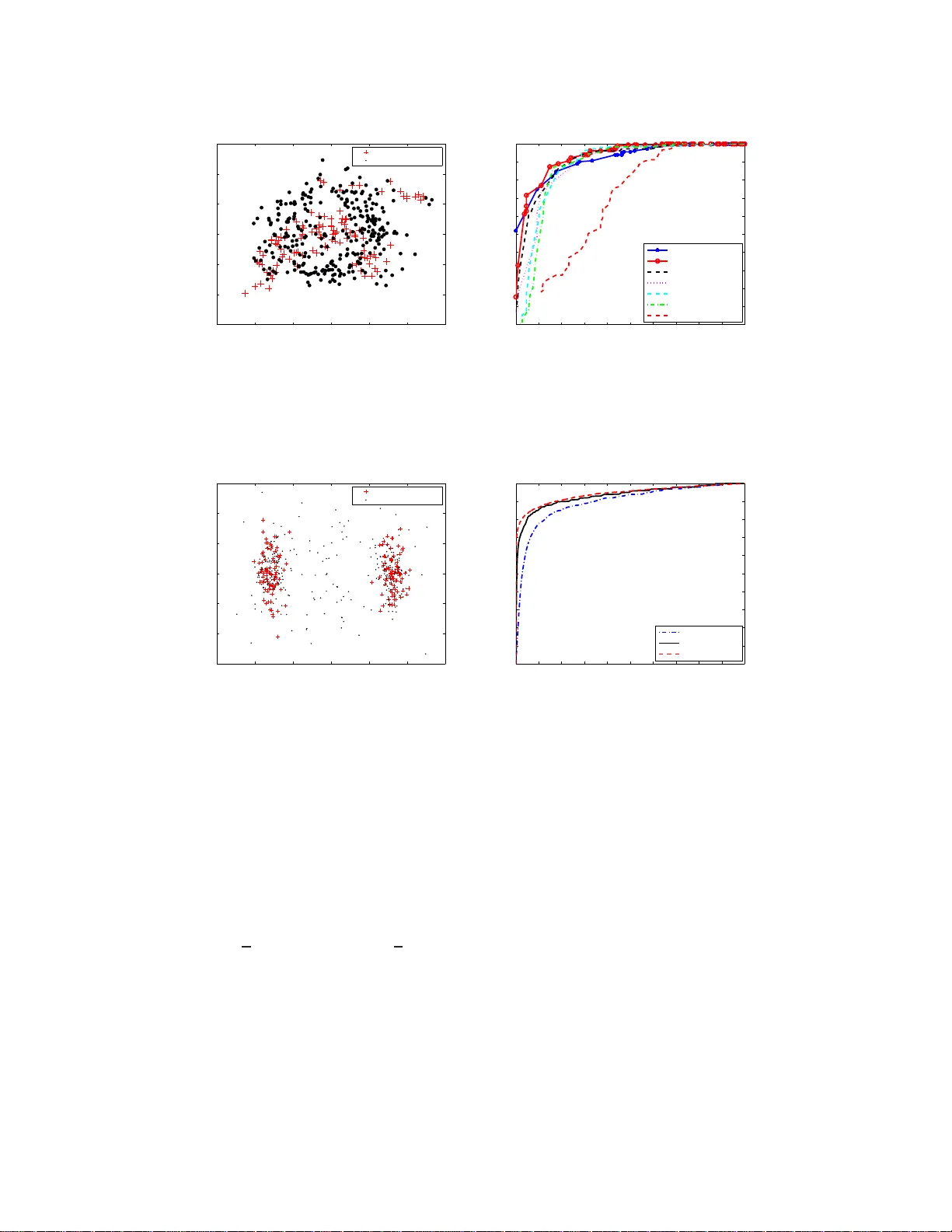
Anomaly Detecti on with Score functions based on Nearest Neighbor Graphs Manqi Zhao ECE Dept. Boston Univ ersity Boston, MA 02215 mqzhao@bu.ed u V enkatesh Saligrama ECE Dept. Boston Univ ersity Boston, MA, 02215 srv@bu.edu Abstract W e propo se a novel non-param etric adapti ve anomaly detec tion algor ithm for high dimensiona l data based on score function s der iv ed fr om nearest neig hbor graphs on n -point nominal data. Anomalies are declared whenever the score of a test sample falls below α , which is supp osed to be the desired false alarm level. The resulting anom aly detector is shown to be asympto tically optimal in that it is u ni- formly most powerful for the spec ified false alarm level, α , fo r the case when the anomaly d ensity is a mix ture of the nom inal an d a k nown density . Our al- gorithm is computationally efficient, be ing linear in dimension an d quad ratic in data size. It does not requ ire choosing complicated tuning param eters or function approx imation classes and it can ad apt to local structur e such as loc al change in dimensiona lity . W e demonstrate the algorith m on both artificial and real data sets in high dimension al feature spaces. 1 Intr oduction Anomaly detection inv olves detec ting statistically sign ificant d eviations of test data from nom inal distribution. In typical applications th e nominal distribution is unknown and generally canno t be reliably estimated from no minal training data d ue to a comb ination of factors such as limited data size and high dimension ality . W e propo se a n adaptive no n-par ametric metho d for ano maly detection based on score function s th at maps d ata samp les to th e inter val [0 , 1] . Our score f unction is d erived fro m a K-ne arest ne ighbor graph (K-NNG) o n n -point nom inal data. Anom aly is declared when ev er the score of a test samp le falls below α ( the desired false alarm error). The ef fica cy of our method rests upon its clo se connec- tion to mu ltiv ariate p -values. In statistical hy pothesis testing, p-v alue is any tran sformatio n of th e feature space to the interv al [0 , 1] that indu ces a uniform distribution o n the nominal data. Whe n test samples with p-values smaller than α are declared as anomalies, f alse alarm error is less than α . W e develop a novel notion of p-values based on measures of le vel sets of likelihood ratio fun ctions. Our notion provides a chara cterization of the optima l anomaly detector, in that, it is uniformly most powerful for a specified false ala rm level for the case whe n the an omaly d ensity is a mixtu re of the nominal and a known density . W e show that our score fun ction is asymptotically consistent, namely , it conv erges to our multi variate p-value as data length appro aches infinity . Anomaly detectio n h as been extensively studied. It is also refe rred to as n ovelty detection [1, 2 ], outlier detection [3], one-class classification [4, 5] and sing le-class classification [6] in the liter- ature. Approac hes to anomaly detection can be g roup ed into se veral c ategories. In parametric approa ches [7] the nomin al den sities are assumed to come from a parameterized family and g en- eralized likelihood r atio tests are used fo r d etecting deviations from nom inal. It is d ifficult to use parametric app roaches when the distribution is unkn own and d ata is limited. A K-nearest neig hbor 1 (K-NN) anoma ly detection appro ach is presented in [ 3, 8] . There an anomaly is d eclared whenever the distance to the K-th nea rest neighbor of the test sample falls outside a threshold. In comparison our anomaly detector utilizes the global information a vailable from the entire K-NN graph to detect deviations from th e no minal. In addition it has p rovable op timality proper ties. Learnin g theor etic approa ches attempt to find decision regions, based on nom inal data, that separate nom inal instances from their outliers. Th ese include o ne-class SVM o f Sch ¨ o lkopf et. al. [9] where the basic id ea is to map the tr aining data into the kernel space and to sepa rate the m from the o rigin with m axi- mum margin . Other algorith ms along this line o f r esearch inclu de supp ort vector d ata de scription [10], linear prog ramming app roach [1], an d single class minimax probab ility machin e [1 1]. While these appr oaches provide impressive compu tationally ef ficient solutions on r eal data, it is gener ally difficult to precisely relate tun ing parameter choices to desired false alarm pro bability . Scott and Nowak [ 12] derive decision r egions based on min imum volume (M V) sets, which does provide T ype I an d T ype II error control. They appr oximate (in approp riate fun ction classes) lev el sets of the unknown nom inal multi variate d ensity from training samples. Related work by Hero [13] b ased on geometric entro pic minimization (GE M) detects outliers by co mparing test samples to the mo st concentr ated su bset of po ints in the tr aining sample. This most con centrated set is th e K -point m inimum spann ing tree(M ST) f or n -po int n ominal d ata and co n verges asymp totically to the minimu m entropy set (wh ich is a lso the MV set). Ne verth eless, computing K -MST fo r n -po int data is ge nerally intractab le. T o o vercome these comp utational limitations [13] pr oposes he uristic greedy algorithm s based on leave-one out K-NN graph , which while inspired by K -MST algorithm is no longer provably optimal. Our appro ach is r elated to these latter tec hnique s, namely , M V sets of [12] and GEM appro ach of [13]. W e de velop score functions on K-NNG which turn out to be the empirical estimates o f the volume of the MV sets containing the test point. The volume, which is a real num ber, is a sufficient statistic for en suring optima l guaran tees. I n this way we av oid explicit high-d imensional level set computation . Y et our a lgorithms lead to statistically optimal solutio ns with the ability to control false alarm and miss error probabilities. The main features of ou r anom aly detector are su mmarized. (1) Like [13] our algorith m scales linearly with dimension and quad ratic with data size and can be applied to high dimensional feature spaces. (2) Like [1 2] ou r algorith m is prov ab ly o ptimal in that it is unifo rmly most p owerful fo r the specified false alarm le vel, α , f or the case that the anomaly density is a mixtur e of the nomin al and any oth er density ( not necessarily uniform). (3) W e do not require assumptions of linear ity , smoothne ss, co ntinuity o f the densities or the conv exity of the lev el sets. Furtherm ore, our a lgorithm adapts to the inhe rent manifold structur e or local dimension ality of the nomin al density . (4) Like [1 3] and unlike other lear ning th eoretic app roache s such as [9, 12] we do not require ch oosing com plex tuning parameter s or function appr oximation classes. 2 Anomaly Detection Algorithm: Score funct ions based on K -NNG In this section we p resent our basic algo rithm dev oid of any statistical con text. Statistical a nalysis appears in Section 3. Let S = { x 1 , x 2 , · · · , x n } be the no minal train ing set of size n belonging to the unit cube [0 , 1] d . For notational convenience we use η and x n +1 interchang eably to denote a test point. Our task is to declare wheth er the test point is consistent with nominal d ata or d eviates from the nom inal d ata. If the test point is an anomaly it is assumed to com e from a mixtur e of nomin al distribution underlying the tra ining data and another known density (see Section 3). Let d ( x, y ) be a distance functio n denoting the distance between any two p oints x, y ∈ [0 , 1] d . For simplicity we denote the distances by d ij = d ( x i , x j ) . In the simp lest case we assume th e distan ce function to b e Euclidean . Howe ver, we also consider geod esic distances to exploit the underly- ing manifold structu re. The g eodesic distance is define d as the s hortest distance on the manifold. The Geod esic Learning alg orithm, a subrou tine in Isomap [ 14, 15] can b e used to efficiently and consistently estimate the geod esic distances. In additio n by means of selecti ve weighting o f d iffer - ent coor dinates note that the distance fun ction could a lso accoun t for pronou nced chan ges in local dimensiona lity . This can be accomplished for in stance th rough Mahalano bis distances or as a by produ ct of local linear em beddin g [16]. Howe ver, we skip the se details her e and assume th at a suitable distance metric is chosen. Once a distance function is defined our next step is to form a K nearest neighbor graph (K-NNG) or alternatively an ǫ neighbor graph ( ǫ -NG). K-NNG is formed by con necting each x i to the K closest 2 points { x i 1 , · · · , x i K } in S − { x i } . W e then sor t the K nearest d istances fo r each x i in increasing order d i,i 1 ≤ · · · ≤ d i,i K and denote R S ( x i ) = d i,i K , that is, the distance from x i to its K - th nearest neighbor . W e co nstruct ǫ -N G where x i and x j are connected if and only if d ij ≤ ǫ . In th is case we define N S ( x i ) as the degree of point x i in the ǫ -NG. For th e si mple case when the anomalou s den sity is an arbitrary mixture of nomin al and unifor m density 1 we consider the following two score functions associated with the two grap hs K-NNG and ǫ -NNG respectively . Th e score functions map the test data η to the interval [0 , 1] . K-LPE: ˆ p K ( η ) = 1 n n X i =1 I { R S ( η ) ≤ R S ( x i ) } (1) ǫ -LPE: ˆ p ǫ ( η ) = 1 n n X i =1 I { N S ( η ) ≥ N S ( x i ) } (2) where I {·} is the indicator function. Finally , given a pre-defined significance l ev el α (e.g., 0 . 05 ), we declare η to be anomalous if ˆ p K ( η ) , ˆ p ǫ ( η ) ≤ α . W e call this algorithm Localized p- value Estimation (LPE) alg orithm. This choice is motiv ated by its close con nection to multi variate p-values(see Section 3). The score fun ction K-LPE (or ǫ - LPE) m easures the r elativ e conc entration of p oint η com pared to the training set. Section 3 establishes that the scor es for nom inally generated data is asympto tically unifor mly d istributed in [0 , 1] . Scores for anomalous data are clu stered arou nd 0 . Hence when scores below level α are declare d as anomalous th e false alar m err or is smaller than α asympto tically (sin ce the integral of a uniform distrib ution from 0 to α is α ). Bivariate Gaussian mixture distribution −6 −4 −2 0 2 4 −6 −5 −4 −3 −2 −1 0 1 2 3 4 5 anomaly detection via K−LPE, n=200, K=6, α =0.05 −6 −4 −2 0 2 4 −6 −5 −4 −3 −2 −1 0 1 2 3 4 5 level set at α =0.05 labeled as anomaly labeled as nominal 0 0.2 0.4 0.6 0.8 1 0 2 4 6 8 10 12 empirical distribution of the scoring function K−LPE value of K−LPE empirical density nominal data anomaly data α =0.05 Figure 1: Left : L ev el sets of the no minal biv ariate Gaussian mixture d istribution used to il lustrate the K- LPE algorithm. Middle : Results of K-LPE with K = 6 and Euclidean distance metric for m = 150 test points drawn from a equal mixture of 2D uniform and the (nominal) biv ariate dist ributions. Scores for the test points are based on 200 nominal training samples. Scores falling below a threshold lev el 0 . 05 are declared as anomalies. The dotted contour corresponds t o the exact biv ariate Gaussian density lev el set at lev el α = 0 . 05 . Right : The empirical distribution of the test point scores associated with t he bi variate Gaussian appear to be uniform while scores for the test points drawn from 2D un iform distribution cluster aroun d zero. Figure 1 illustrates the use of K-LPE algo rithm fo r anom aly detection wh en th e no minal data is a 2D Gaussian mixture. T he middle panel of figure 1 sho ws the detection results based on K-LPE are consistent with the theoretica l contour for sig nificance level α = 0 . 05 . The right panel of figure 1 shows th e empirical distribution (derived from the kernel density estimation ) of the scor e function K-LPE for the nominal (solid blue) an d the anom aly (dashed red) data. W e can see that the curve for the n ominal d ata is appro ximately uniform in the in terval [0 , 1] and the curve f or the anomaly data has a peak at 0 . Th erefor e cho osing the threshold α = 0 . 05 will approx imately con trol the T yp e I error within 0 . 05 an d minimize the T ype II error . W e also take note of the inherent robustness of our algorithm . As seen fr om the figure (right) small ch anges in α lead to small changes in actual false alarm and miss le vels. 1 When the mixing density is not uniform but, say f 1 , the score functions must be modified to ˆ p K ( η ) = 1 n P n i =1 I  1 R S ( η ) f 1 ( η ) ≤ 1 R S ( x i ) f 1 ( x i ) ff and ˆ p ǫ ( η ) = 1 n P n i =1 I  N S ( η ) f 1 ( η ) ≥ N S ( x i ) f 1 ( x i ) ff for the two graphs K-NNG and ǫ -NNG respectiv ely . 3 T o summa rize the above discussion, our LPE algorithm has three steps: (1) Inputs: Significance lev el α , distance metric (Euclidean, geodesic, weighted etc.). (2) Score computa tion: Con struct K-NNG (or ǫ -NG) based on d ij and compute the score func tion K-LPE from Equation 1 (or ǫ -LPE from Equation 2). (3) Make Decision: Declare η to be anomalous if and only if ˆ p K ( η ) ≤ α (or ˆ p ǫ ( η ) ≤ α ). Computational Co mplexity: T o com pute each pairwise distance requires O(d) o perations; and O( n 2 d ) operations for all the nodes in the training set. In the worst-case comp uting the K-NN graph (for small K ) and the functions R S ( · ) , N S ( · ) requ ires O( n 2 ) operatio ns over all the n odes in the training data. Finally , computing the score for each test data requires O(nd+n) operations(given th at R S ( · ) , N S ( · ) have already been comp uted). Remark: LPE is fundam entally different from non-par ametric den sity estimation or lev el set esti- mation schem es (e. g., MV -set). These appr oaches inv olve explicit estimation o f h igh dime nsional quantities and thus hard to apply in high dimen sional pro blems. By computing scor es for each test sample w e a void high -dimen sional computation. Furthermore, as we will see in the following sec- tion the scor es are estimates of m ultiv ariate p-values. These tu rn ou t to be suf ficient statistics f or optimal anomaly detection. 3 Theory: Consistency of LPE A statistical framew o rk for the anomaly detection problem is presented in this section. W e establish that anomaly d etection is equivalent to thresholding p- values for multiv ariate data. W e will then show t hat the scor e functions dev eloped in the previous section is an asymptotically consistent esti- mator of the p-v alues. Consequently , it will follow that the strategy of declaring an anomaly when a test sample has a low score is asympto tically optimal. Assume th at the d ata belong s to the d-dim ensional unit cube [0 , 1] d and the n ominal d ata is sam- pled from a mu ltiv ariate d ensity f 0 ( x ) supported on the d-dimen sional un it cub e [0 , 1] d . Anomaly detection can be f ormulated as a com posite hypoth esis testing p roblem. Supp ose test data, η com es from a mixture d istribution, namely , f ( η ) = (1 − π ) f 0 ( η ) + π f 1 ( η ) wh ere f 1 ( η ) is a mixing density supported on [0 , 1] d . Ano maly detection in volves testing the nominal hyp otheses H 0 : π = 0 versus the alternative (anomaly) H 1 : π > 0 . The go al is to maximize the d etection power subject to false alarm lev el α , namely , P ( declare H 1 | H 0 ) ≤ α . Definition 1. Let P 0 be the nomin al probab ility measure and f 1 ( · ) be P 0 measurable. Suppose the likelihood ratio f 1 ( x ) /f 0 ( x ) does not have non -zer o flat spots o n any open b all in [0 , 1] d . Define the p-value of a data point η as p ( η ) = P 0  x : f 1 ( x ) f 0 ( x ) ≥ f 1 ( η ) f 0 ( η )  Note that the definition natur ally a ccounts for sin gularities which may ar ise if the supp ort of f 0 ( · ) is a lower dimension al ma nifold. In this case we encou nter f 1 ( η ) > 0 , f 0 ( η ) = 0 an d the p-value p ( η ) = 0 . Here ano maly is alw ays declared( low scor e). The above formula can be tho ught of as a mapping o f η → [0 , 1] . Furthermor e, the distribution of p ( η ) u nder H 0 is unif orm on [0 , 1] . Howev er , as noted in the introductio n th ere are other such trans- formation s. T o build intuition about the above transfo rmation and its utility consider th e following example. When the m ixing d ensity is uniform , namely , f 1 ( η ) = U ( η ) where U ( η ) is uniform over [0 , 1] d , note th at Ω α = { η | p ( η ) ≥ α } is a d ensity le vel set at level α . It is well known (see [12]) that such a density level set is equiv a lent to a minim um volume set of le vel α . The minimu m volume set a t level α is known to be the unif ormly most powerful decision region for testing H 0 : π = 0 versus the alternati ve H 1 : π > 0 (see [13, 12]). The generalization to arbitrary f 1 is describ ed next. Theorem 1. The uniformly most p owerful test for testing H 0 : π = 0 versus the alternative (anoma ly) H 1 : π > 0 at a pres cribed level α o f significan ce P ( de clar e H 1 | H 0 ) ≤ α is: φ ( η ) =  H 1 , p ( η ) ≤ α H 0 , o therwise 4 Pr oof. W e provide the main idea fo r the proo f. First, m easure theoretic arguments are used to establish p ( X ) as a random variable over [0 , 1] under bo th nomin al and anomalou s distributions. Next when X d ∼ f 0 , i.e., distributed with nom inal density it follows that the random variable p ( X ) d ∼ U [0 , 1] . When X d ∼ f = (1 − π ) f 0 + π f 1 with π > 0 the random variable, p ( X ) d ∼ g wher e g ( · ) is a monotonically decre asing P DF supported on [0 , 1] . Consequently , the unif ormly most powerful test for a significance level α is to declare p-values smaller than α as anom alies. Next we derive the relation ship between the p- values and ou r sco re f unction . By d efinition, R S ( η ) and R S ( x i ) ar e correlated because the neighb orho od of η and x i might o verlap. W e mod ify ou r algorithm to simp lify ou r analysis. W e assume n is odd (say) a nd can be written a s n = 2 m + 1 . W e divide training set S into two parts: S = S 1 ∩ S 2 = { x 0 , x 1 , · · · , x m } ∩ { x m +1 , · · · , x 2 m } W e modify ǫ -LPE to ˆ p ǫ ( η ) = 1 m P x i ∈ S 1 I { N S 2 ( η ) ≥ N S 1 ( x i ) } (or K -LPE to ˆ p K ( η ) = 1 m P x i ∈ S 1 I { R S 2 ( η ) ≤ R S 1 ( x i ) } ). Now R S 2 ( η ) an d R S 1 ( x i ) are independ ent. Furthermo re, we assume f 0 ( · ) satisfies the following tw o smo othness conditio ns: 1. th e Hessian matrix H ( x ) of f 0 ( x ) is al ways domin ated by a matrix with l argest eigen value λ M , i.e., ∃ M s.t. H ( x )  M ∀ x a nd λ max ( M ) ≤ λ M 2. I n the support of f 0 ( · ) , its value is always lo we r bound ed by some β > 0 . W e have the follo wing theorem. Theorem 2. Consider the setup ab ove with the training d ata { x i } n i =1 generated i.i.d. fr om f 0 ( x ) . Let η ∈ [0 , 1 ] d be a n a rbitrary test sample. It follows that for a suitab le choice K an d under the above smoothness conditions, | ˆ p K ( η ) − p ( η ) | n →∞ − → 0 almost sur ely , ∀ η ∈ [0 , 1] d For simplicity , we limit ourselves to the case when f 1 is unif orm. Th e proo f of Theo rem 2 con sists of two steps: • W e sho w that the e x pectation E S 1 [ ˆ p ǫ ( η )] n →∞ − → p ( η ) (Lem ma 3 ). Th is result is then e x- tended to K-LPE (i.e. E S 1 [ ˆ p K ( η )] n →∞ − → p ( η ) ) in Lem ma 4. • Next we show that ˆ p K ( η ) n →∞ − → E S 1 [ ˆ p K ( η )] via con centration inequality (Lemma 5). Lemma 3 ( ǫ -LPE) . B y picking ǫ = m − 3 5 d q d 2 π e , with pr obab ility at least 1 − e − β m 1 / 15 / 2 , l m ( η ) ≤ E S 1 [ ˆ p ǫ ( η )] ≤ u m ( η ) (3) wher e l m ( η ) = P 0 { x : ( f 0 ( η ) − ∆ 1 ) (1 − ∆ 2 ) ≥ ( f 0 ( x ) + ∆ 1 ) (1 + ∆ 2 ) } − e − β m 1 / 15 / 2 u m ( η ) = P 0 { x : ( f 0 ( η ) + ∆ 1 ) (1 + ∆ 2 ) ≥ ( f 0 ( x ) − ∆ 1 ) (1 − ∆ 2 ) } + e − β m 1 / 15 / 2 ∆ 1 = λ M m − 6 / 5 d / (2 π e ( d + 2)) and ∆ 2 = 2 m − 1 / 6 . Pr oof. W e only prove the lo wer boun d since the upper b ound follows along similar lines. B y inte r- changin g the expectation with the summation, E S 1 [ ˆ p ǫ ( η )] = E S 1 " 1 m X x i ∈ S 1 I { N S 2 ( η ) ≥ N S 1 ( x i ) } # = 1 m X x i ∈ S 1 E x i E S 1 \ x i h I { N S 2 ( η ) ≥ N S 1 ( x i ) } i = E x 1 [ P S 1 \ x 1 ( N S 2 ( η ) ≥ N S 1 ( x 1 ))] 5 where the last inequality follows from the symm etric structure of { x 0 , x 1 , · · · , x m } . Clearly the ob jectiv e o f the pr oof is to sho w P S 1 \ x 1 ( N S 2 ( η ) ≥ N S 1 ( x 1 )) n →∞ − → I { f 0 ( η ) ≥ f 0 ( x 1 ) } . Skipping te chnical details, th is can b e accomplished in two steps. (1) Note th at N S ( x 1 ) is a bino mial random variable with success p robab ility q ( x 1 ) := R B ǫ f 0 ( x 1 + t ) d t . This relates P S 1 \ x 1 ( N S 2 ( η ) ≥ N S 1 ( x 1 )) to I { q ( η ) ≥ q ( x 1 ) } . (2) W e relate I { q ( η ) ≥ q ( x 1 ) } to I { f 0 ( η ) ≥ f 0 ( x 1 ) } based on the fu nction smoothne ss cond ition. The details of these two steps are shown i n the below . Note that N S 1 ( x 1 ) ∼ Bino m ( m, q ( x 1 )) . By Chern off bou nd of binomial distrib u tion, we ha ve P S 1 \ x 1 ( N S 1 ( x 1 ) − mq ( x 1 ) ≥ δ ) ≤ e − δ 2 2 mq ( x 1 ) that is, N S 1 ( x 1 ) is concentra ted arou nd mq ( x 1 ) . This implies, P S 1 \ x 1 ( N S 2 ( η ) ≥ N S 1 ( x 1 )) ≥ I { N S 2 ( η ) ≥ mq ( x 1 )+ δ x 1 } − e − δ 2 x 1 2 mq ( x 1 ) (4) W e choo se δ x 1 = q ( x 1 ) m γ ( γ w ill be specified later ) and reformu late equatio n (4) as P S 1 \ x 1 ( N S 2 ( η ) ≥ N S 1 ( x 1 )) ≥ I  N S 2 ( η ) m V ol ( B ǫ ) ≥ q ( x 1 ) V ol ( B ǫ ) ( 1+ 2 m 1 − γ ) ff − e − q ( x 1 ) m 2 γ − 1 2 (5) Next, we relate q ( x 1 )( or R B ǫ f 0 ( x 1 + t ) d t ) to f 0 ( x 1 ) via the T aylor’ s e xpansion an d t he smooth ness condition of f 0 ,      R B ǫ f 0 ( x 1 + t ) d t V ol ( B ǫ ) − f 0 ( x 1 )      ≤ λ M 2 · 1 V ol ( B ǫ ) Z B ǫ k t k 2 d t = λ M ǫ 2 2 d ( d + 2) (6) and then equation (5) become s P S 1 \ x 1 ( N S 2 ( η ) ≥ N S 1 ( x 1 )) ≥ I  N S 2 ( η ) m V ol ( B ǫ ) ≥ “ f 0 ( x 1 )+ λ M ǫ 2 2 d ( d +2) ” ( 1+ 2 m 1 − γ ) ff − e − q ( x 1 ) m 2 α − 1 2 By applying the same steps to N S 2 ( η ) as equation 4 (Chernoff bou nd) and equation 6 (T a ylor’ s explansion), we ha ve with prob ability at least 1 − e − q ( η ) m 2 α − 1 2 , E x 1 [ P S 1 \ x 1 ( N S 2 ( η ) ≥ N S 1 ( x 1 ))] ≥ P x 1 „ f 0 ( η ) − λ M ǫ 2 2 d ( d +2) « “ 1 − 2 m 1 − γ ” ≥ „ f 0 ( x 1 )+ λ M ǫ 2 2 d ( d +2) « “ 1+ 2 m 1 − γ ” ff − e − q ( x 1 ) m 2 α − 1 2 Finally , by choosing ǫ 2 = m − 6 5 d · d 2 π e and γ = 5 / 6 , we prove the lemma. Lemma 4 ( K -LPE) . By p icking K =  1 − 2 m − 1 / 6  m 2 / 5 ( f 0 ( η ) − ∆ 1 ) , with pr obab ility at least 1 − e − β m 1 / 15 / 2 , l m ( η ) ≤ E S 1 [ ˆ p K ( η )] ≤ u m ( η ) (7) Pr oof. The pro of is very similar to the proo f to Lemma 3 and we only give a brief outline here. Now the o bjective is to show P S 1 \ x 1 ( R S 2 ( η ) ≤ R S 1 ( x 1 )) n →∞ − → I { f 0 ( η ) ≥ f 0 ( x 1 ) } .The basic idea is to use the r esult of Lem ma 3. T o accom plish this, we note that { R S 2 ( η ) ≤ R S 1 ( x 1 ) } contains th e events { N S 2 ( η ) ≥ K } ∩ { N S 1 ( x 1 ) ≤ K } , or equi valently { N S 2 ( η ) − q ( η ) m ≥ K − q ( η ) m } ∩ { N S 1 ( x 1 ) − q ( x 1 ) m ≤ K − q ( x 1 ) m } (8) By the tail probability of Binomial distribution, the probab ility of the above two e vents conv erges to 1 exponen tially fast if K − q ( η ) m < 0 and K − q ( x 1 ) m > 0 . By using th e same two-step boundin g technique s de veloped in the proof to Lemma 3, these two inequalities are implied by K − m 2 / 5 ( f 0 ( η ) − ∆ 1 ) < 0 and K − m 2 / 5 ( f 0 ( x 1 ) + ∆ 1 ) > 0 Therefo re if we choo se K =  1 − 2 m − 1 / 6  m 2 / 5 ( f 0 ( η ) − ∆ 1 ) , we have with pr obability at least 1 − e − β m − 1 / 15 / 2 , P S 1 \ x 1 ( R S 2 ( η ) ≤ R S 1 ( x 1 )) ≥ I { ( f 0 ( η ) − ∆ 1 )(1 − ∆ 2 ) ≥ ( f 0 ( x 1 )+∆ 1 )(1+∆ 2 ) } − e − β m − 1 / 15 / 2 6 Remark: Lemm a 3 and Lemma 4 were proved with specific choices for ǫ and K . Howev er , ǫ and K can be chosen in a range of values, b ut will lead to different lo wer and up per bounds. W e will show in Section 4 throu gh simulatio ns that our LPE algo rithm is ge nerally ro bust to ch oice of par ameter K . Lemma 5. S uppo se K = cm 2 / 5 and denote ˆ p K ( η ) = 1 m P x i ∈ S 1 I { R S 2 ( η ) ≤ R S 1 ( x i ) } . W e h ave P 0 ( | E S 1 [ ˆ p K ( η )] − ˆ p K ( η ) | > δ ) ≤ 2 e − 2 δ 2 m 1 / 5 c 2 γ 2 d wher e γ d is a constant and is defined as the minimal number of cones center ed at the origin of angle π / 6 that cover R d . Pr oof. W e can not apply Law of Large Numb er in this case beca use I { R S 2 ( η ) ≤ R S 1 ( x i ) } are cor- related. Instead, we need to use th e mo re generalized conc entration- of-measu re inequ ality such as M acDiarmid’ s ineq uality[17]. Den ote F ( x 0 , · · · , x m ) = 1 m P x i ∈ S 1 I { R S 2 ( η ) ≤ R S 1 ( x i ) } . Fr om Corollary 11.1 in [18], sup x 0 , ··· ,x m ,x ′ i | F ( x 0 , · · · , x i , · · · , x m ) − F ( x 0 , · · · , x ′ i , · · · , x n ) | ≤ K γ d /m (9) Then the lemma directly follows from app lying McDiarmid’ s inequality . Theorem 2 dire ctly fo llows from the com bination of Lem ma 4 and Lemma 5 and a standard ap pli- cation of the first Borel-Cantelli lemma. W e hav e used Euclidean distance in Th eorem 2. When the support of f 0 lies on a lo wer dimensional man ifold (say d ′ < d ) ado pting the geode sic metric leads to faster con vergence. It turns out that d ′ replaces d in the expression for ∆ 1 in Lemma 3. 4 Experiments W e apply our method on both artificial an d real-world data . Our meth od enables p lotting the entire R OC cur ve by v ary ing the thresholds on our scores. T o test the sensiti v ity of K-LPE to parameter c hanges, we first r un K -LPE o n the be nchmar k ar- tificial data-set B anana [19] with K varying fro m 2 to 12 . Bana na dataset contains points with their labels( +1 o r − 1 ). W e rand omly pick 109 points with +1 label and regard th em as the nom inal training data. The test data co mprises of 10 8 +1 data and 183 − 1 data (grou nd truth) and the alg o- rithm is supposed to pred ict +1 data as “nominal” and − 1 data as “an omaly”. See Figu re 2 (a) for the config uration of the tr aining poin ts and test po ints. Scor es compu ted for test set using Equation 1 is oblivious to tru e f 1 density ( − 1 labels). E uclidean distance metric is adopted for this example. False alarm (also called false positive) is de fined as the perce ntage of no minal points tha t are p re- dicted as ano maly by the algo rithm. T o control false alarm at le vel α , point with score < α is predicted as anomaly . Empirical f alse alarm and true positi ves (percentag e of anomalies declared as anomaly) can be compu ted f rom ground truth. W e vary α to ob tain the empirica l R OC cur ve. W e follow this procedure for all the other experiments in this section. W e are relatively in sensitiv e to K as shown in Figur e 2(b). For compariso n we plot the empirical R OC curve of the one-c lass SVM of [ 9]. Th ere are two tuning parameters in OC-SVM — bandwidth c (we use RB F kern el) and ν ∈ (0 , 1) (which is supposed to control F A). Note that training data does not contain − 1 lab els and this implies we ca n ne ver make use o f − 1 lab els to c ross-validate, or, to op timize over the cho ice of pair ( c, ν ) . In our OC- SVM implementation , by following th e same procedure, we can obtain the empirical R OC cu rve by varying ν but fixing a certain ba ndwidth c . Finally we iterated over different c to ob tain the best (in terms of A UC) R OC cu rve an d it tu rns out to be c = 1 . 5 . Fixing c for entire R OC is equ iv alent to fixing K in our score function. Note th at in real p ractice what can be done is even worse than this implementatio n becau se ther e is also no natural way to optim ize over c without being rev ealed th e − 1 labels. In Figure 2(b) , we can see that our algorithm is consistently better th an o ne-class SVM on the Banana dataset. Furtherm ore, we fou nd that choosing suitable tun ing parameter s to contro l false alarms is gener ally dif ficult in the on e-class SVM approac h. In our appr oach if we set α = 0 . 05 we 7 −3 −2 −1 0 1 2 3 −3 −2 −1 0 1 2 3 Nominal training data Unlabeled test data (a) Configuratio n of banana data 0 0.1 0.2 0.3 0.4 0.5 0.6 0.7 0.8 0.9 1 0 0.1 0.2 0.3 0.4 0.5 0.6 0.7 0.8 0.9 1 false positives true positives banana data set ROC of LPE (K=2) ROC of LPE (K=4) ROC of LPE (K=6) ROC of LPE (K=8) ROC of LPE (K=10) ROC of LPE (K=12) ROC of one−class SVM (b) SVM vs. K-L PE for Banana Data Figure 2: Performance Robustness of L PE;(a) The configuration of t he nominal training points (red ‘+’) and unlabeled t est points (black ‘ • ’) for the banana dataset [ 19]; (b) Empirical ROC curve of K -LPE on the banana dataset with K = 2 , 4 , 6 , 8 , 10 , 12 (with n = 400 ) vs the empirical R O C curv e of one class SVM de velo ped in [9]. −15 −10 −5 0 5 10 15 −15 −10 −5 0 5 10 15 Nominal training data Unlabeled test data (a) Configuratio n of data 0 0.1 0.2 0.3 0.4 0.5 0.6 0.7 0.8 0.9 1 0 0.1 0.2 0.3 0.4 0.5 0.6 0.7 0.8 0.9 1 false positives true positives 2D Gaussian mixture ROC of LPE(n=40) ROC of LPE(n=160) Clairvoyant ROC (b) Clairvoyant vs. K-LPE Figure 3: Clairvo yant R OC curve vs. K-LPE; (a) Configuration of t he nominal training points and unlabeled test points for the data giv en by Equation 10; (b) A v eraged (ov er 15 trials) empirical R OC curves of K -LPE algorithm vs clairvoyant ROC curve (when f 0 is giv en by Equation 10) for K = 6 and for different values of n ( n = 40 , 160 ). get empiric al F A = 0 . 06 and fo r α = 0 . 08 , emp irical F A = 0 . 0 9 . For OC-SVM we can n ot see any natural way of picking c and ν to contr ol F A rate based only on training data. In Fi gure 3, we apply o ur K -LPE to an other 2D artificial example wh ere the no minal distribution f 0 is a mixture Gaussian an d the an omalou s d istribution is very close to u niform (see Fig ure 3(a) f or their configur ation): f 0 ∼ 1 2 N  8 0  ,  1 0 0 9  + 1 2 N  − 8 0  ,  1 0 0 9  , f 1 ∼ N  0 ,  49 0 0 49  (10) In this example, we can exactly com pute the optimal R OC curve. W e call this curve the Clairvoyant R OC (the red dashed curve in Figure 3(b )). The other two c urves are averaged (over 15 trials) empirical R OC curves with respect to different sizes of training sample ( n = 40 , 160 ) for K = 6 . Larger n results in better ROC cur ve. W e see that for a relati vely small training set of size 160 the av erage empirical R OC curve is very close to the clairvoyant R OC curve. Next, w e ran LPE on three real-world data sets: Wine , I onosphere [2 0] and MNIST US Postal Service ( USPS ) d atabase o f handwritten d igits. Th e procedure and setup of the experimen ts is almost the same as the that of the Banana data set. Howe ver, there are two differences. (1) If the number of dif f erent labels is greater than two, we always treat p oints with on e particular labe l as 8 nominal( +1 ) and regard the points with other labels as anomalo us( − 1 ). For e xample, for the USPS dataset, we regard instances of dig it 0 as nom inal trainin g samples and instances of d igits 1 , · · · , 9 as a nomaly . ( 2) For high dim ensional d ata set, the data p oints a re norm alized to be within [0 , 1] d and we use geode sic distance [14 ](instead of Euclidean distance) as the input to LPE. 0 0.1 0.2 0.3 0.4 0.5 0.6 0.7 0.8 0.9 1 0 0.1 0.2 0.3 0.4 0.5 0.6 0.7 0.8 0.9 1 false positive true positive 0 0.1 0.2 0.3 0.4 0.5 0.6 0.7 0.8 0.9 1 0 0.1 0.2 0.3 0.4 0.5 0.6 0.7 0.8 0.9 1 false positive true positive 0 0.1 0.2 0.3 0.4 0.5 0.6 0.7 0.8 0.9 1 0 0.1 0.2 0.3 0.4 0.5 0.6 0.7 0.8 0.9 1 false positive true positive (a) Wine (b) Ionosphere (c) USPS Figure 4: R OC curv es on real datasets via L P E ; (a) Wine dataset wi th D = 13 , n = 39 , ǫ = 0 . 9 ; (b) Ionosphere dataset with D = 34 , n = 175 , K = 9 ; (c) USPS dataset with D = 256 , n = 400 , K = 9 . The R OC curves o f these three data sets are shown in Figure 4. In Wine dataset, the dimensio n of the feature space is 13 . The training set is comp osed of 39 data points and we apply the ǫ -LPE algor ithm with ǫ = 0 . 9 . The test set is a mixture of 20 nom inal points and 158 anomaly points (gro und truth). In Ionosph ere d ataset, the dimension of the feature space is 34 . T he trainin g set is composed of 175 data points and we apply the K -LPE alg orithm with K = 9 . The test set is a m ixture of 50 nominal points and 12 6 anom aly poin ts (gr ound truth). In USPS dataset, the dimension of the feature space is 16 × 16 = 256 . The trainin g set is comp osed of 40 0 data poin ts and we apply the K -LPE algor ithm with K = 9 . The test set is a mix ture of 367 n ominal po ints and 33 an omaly points (grou nd truth) . For comp arison purposes we note that for th e USP S data set by setting α = 0 . 5 we get em pirical false-positiv e 6 . 1% and empirical false alarm rate 5 . 7% (In contrast F P = 7% and F A = 9% with ν = 5% for OC-SVM as r eported in [9]). Practically we find that K -LPE is m ore prefer able to ǫ - LPE du e to easiness of c hoosing the p arameter K . W e find that th e value o f K is relati vely indepen dent of dimension d . A s a rule of thumb we found that setting K a round n 2 / 5 was generally effecti ve. 5 Conclusion In th is paper, we p roposed a novel non-param etric ad aptive an omaly detection a lgorithm w hich leads to a c omputatio nally ef ficient solution with p rovable optimality gu arantees. Ou r algorith m takes a K-nearest neighb or graph as an input and produce s a score for each test point. Sco res turn out to be empirical estimates o f the volume of min imum volume level sets c ontaining the test p oint. While minimum volume level sets provid e an optim al characteriz ation for ano maly detectio n, they are high dimensional q uantities and generally d ifficult to reliably compu te in high dimensional feature spaces. Nevertheless, a sufficient statistic for op timal trad eoff between false alar ms an d misses is the volume of th e MV set itself, which is a r eal nu mber . By computing score func tions we avoid computin g high dimensio nal q uantities and still ensure optimal control of false alarms and misses. The compu tational cost of our algorith m scales linearly in dimension and quadratically in data size. Refer ences [1] C. Campbell and K. P . Bennett, “ A linear programming approac h to nov elty detection, ” in Advances in Neural Information Pr ocessing Systems 13 . MIT Press, 2001, pp. 395–40 1. [2] M. M arkou and S. Singh, “No velty detection: a re view – part 1: statist ical approa ches, ” S ignal Pr ocessing , vol. 8 3, pp. 2481–2497 , 2003. [3] R. Ramaswamy , R. Rastogi, and K. Shim, “Efficient algorithms for mining outliers from large data sets, ” in Pr oceeding s of the ACM SIGMOD Confer ence , 2000. 9 [4] R. V ert and J. V ert, “Consistency and co n vergen ce rates of one-class svms and related algorithms, ” Journa l of Machine Learning Resear ch , vol. 7, pp. 817–854, 2006. [5] D. T ax and K. R. M ¨ u ller , “Feature extraction for one-class classifi cation, ” in Artificial neural networks and neural informa tion pr ocessing , Istanbul, TURQUIE, 2003. [6] R. El -Y aniv and M. N isenson, “Optimal singl-class classification strategies, ” in Advance s in Neural In- formation Pr ocessing Systems 19 . MIT Press, 2007. [7] I. V . Nikiforov and M. Basse ville, Detection of abru pt chan ges: theory and a pplications . Prentice-Hall, Ne w Jersey , 1993. [8] K. Zhang, M. Hutter, and H. Jin, “ A new l ocal distance-based outlier detection approach for scattered real-world data, ” March 2009, arXi v:0903.32 57v1[cs.LG]. [9] B. Sch ¨ o lkop f, J. C. Platt, J. Shawe-T aylor, A. J. Smola, and R. Williamson, “Est imating the support of a high-dimension al distribution, ” Neural Computation , vol. 13 , no. 7, pp. 1443–147 1, 2001. [10] D. T ax, “One-class classification: Concept-learning in the absence of counter -examp les, ” Ph.D. disserta- tion, Delft Univ ersity of T echnology , June 2001. [11] G. R. G. Lanckriet, L. E. Ghaoui, and M. I. Jordan, “Robust novelty detection wi th single-class MPM, ” in Neural Information Pr ocessing Systems Confer ence , vol. 18, 2005. [12] C. Scott and R. D. Nowa k, “L earning minimum volume sets, ” Jou rnal of Machine Learning Resear ch , vol. 7 , pp. 665–704 , 2006. [13] A. O. Hero, “Geometric entropy minimization(GEM) for anomaly detection and localization, ” in Neural Information Pr ocessing Systems Con fer ence , vol. 19, 2006 . [14] J. B. T enenbaum, V . de Sil v a, and J. C. Langford, “ A global geometric framework fo nonlinea r dimen- sionality reduction, ” Science , vol. 290, pp. 2319 –2323 , 2000. [15] M. Bernstein, V . D. Silva, J. C. Langford, and J. B. T enenbaum, “Graph approximations to geodesics on embedded manifolds, ” 2000. [16] S. T . R o weis and L. K. S aul, “Nonlinear dimensionality reduction by l ocal linear embedding, ” Science , vol. 2 90, pp. 2323–232 6, 2000. [17] C. McDiarmid, “On the method of bounded dif f erences, ” in Surveys in Combinatorics . Cambridge Univ ersity Pr ess, 1989 , pp. 148–188. [18] L. Devro ye, L. Gy ¨ orfi, and G . Lugosi, A Pr obabilistic Theory of P attern Recognition . Springer V erlag Ne w Y ork, Inc., 1996. [19] “Benchmark repository . ” [Online]. A v ailable: http:// ida.first.fhg.de/projects/bench/bench marks.htm [20] A. Asuncion and D. J. Newman, “UCI machine learning repository , ” 2007. [O nline]. A v ai lable: http://www .ics.uci.edu/$ \ sim$mlearn/ { MLR } epository .html 10