Learning Class-Level Bayes Nets for Relational Data

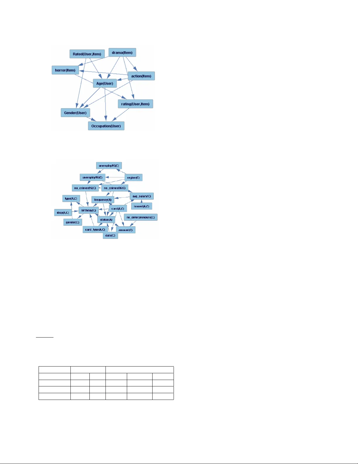
Learning Class-Le vel Bayes Nets for Relational Data Oli ver Schulte, Hassan Khosra vi, Bahareh Bina, Flavia Moser , Martin Ester { oschulte, hkhosrav , bb18,fmoser , ester } @cs.sfu.ca School of Computing Science Simon Fraser Uni versity V ancouver -Burnaby , B.C., Canada Abstract Many databases store data in relational format, with differ - ent types of entities and information about links between the entities. The field of statistical-relational learning (SRL) has dev eloped a number of ne w statistical models for such data. In this paper we focus on learning class-lev el or first-order dependencies, which model the general database statistics ov er attrib utes of linked objects and links (e.g., the percent- age of A grades giv en in computer science classes). Class- lev el statistical relationships are important in themselves, and the y support applications like policy making, strate- gic planning, and query optimization. Most current SRL methods find class-lev el dependencies, b ut their main task is to support instance-le vel predictions about the attributes or links of specific entities. W e focus only on class-level predic- tion, and describe algorithms for learning class-le vel models that are orders of magnitude faster for this task. Our algo- rithms learn Bayes nets with relational structure, lev eraging the efficienc y of single-table nonrelational Bayes net learn- ers. An ev aluation of our methods on three data sets sho ws that they are computationally feasible for realistic table sizes, and that the learned structures represent the statistical infor- mation in the databases well. After learning compiles the database statistics into a Bayes net, querying these statistics via Bayes net inference is faster than with SQL queries, and does not depend on the size of the database. 1 Introduction Many real-w orld applications store data in relational format, with different tables for entities and their links. Standard machine learning techniques are applied to data stored in a single table, that is, in nonrelational, propositional or “flat” format [18]. The field of statistical-relational learning (SRL) aims to extend machine learning algorithms to relational data [8, 3]. One of the major machine learning tasks is to use data to build a generative statistical model for the variables in an application domain [8]. In the single-table learning setting, the goal is often to represent predictiv e dependencies between the attributes of a single individual (e.g., between the intelligence and ranking of a student). In the SRL setting, the goal is often to represent, in addition, dependencies between attributes of dif ferent individuals that are related or linked to each other (e.g., between the intelligence of a student and the difficulty of a course giv en that the student is registered in the course). T ask Description: Modelling Class-Level Dependencies Many SRL models distinguish two different lev els, a class or type dependency model G M and an instance dependency model G I [7, 14, 19]. In a graphical SRL model, the nodes in the instance dependency model represent attributes of indi- viduals or relationships. The nodes in the class dependency model correspond to attributes of the tables. The use of the term “class” here is unrelated to classification; [16] views it as analogous to the concept of class in object-oriented pro- gramming. An example of a class-level probabilistic depen- dency is “among students with high intelligence, the rate of GP A = 4.0 is 80%”. An instance-level prediction would be “giv en that Jack is highly intelligent, the probability that his GP A is 4.0 is 80%”. Thus class-level dependencies are con- cerned with the rates at which events occur , or at which prop- erties hold within a class, whereas instance-lev el dependen- cies are concerned with specific ev ents or the properties of specific entities [11, 1]. In terms of predicate logic, the class- lev el model features terms that inv olve first-order v ariables (e.g., intel ligenc e ( S ) , where S is a variable ranging over a domain like Students ), whereas the instance-le vel graph fea- tures terms that in v olve constants (e.g., intel ligenc e ( jack ) where jack is a constant that denotes a particular student) [3, 14, 5]. T ypically , SRL systems instantiate a class-level model G M with the specific entities, their attributes and their re- lationships in a giv en database to obtain an instance depen- dency graph G I . An important purpose of the instance graph is to support predictions about the attributes of individual en- tities. A key issue for making such predictions is the com- bining problem : how to combine information from different related entities to predict a property of a target entity . Cur- rent SRL model construction algorithms learn class-le vel de- pendencies and instance-level predictions at the same time. What is new about our approach is that we focus on class- lev el v ariables only rather than making predictions about in- dividual entities. W e apply Bayes net technology to design new algorithms especially for learning class-lev el dependen- cies. In experiments our algorithms run at two orders of mag- nitude faster than a benchmark SRL method. Our models thus trade-off tractability of learning with the ability to an- swer queries about individual entities. Applications. Examples of applications that provide motiv ation for the class-level statistical models include the following. 1. P olicy making and strate gic planning. A univ ersity ad- ministrator may wish to know which program charac- teristics attract high-ranking students in general, rather than predict the rank of a specific student in a specific program. 2. Query optimization is one of the applications of SRL where a statistical model predicts a probability for giv en table join conditions that can be used to infer the size of the join result [9]. Estimating join sizes is a key problem for database query optimization. In queries that in v olve se veral tables being joined together , the ideal scenario is to hav e smaller intermediate joins [17]. A class-lev el statistical model may be used for estimating frequency counts in the database to select smaller joins, and so to optimize the speed of answer- ing queries by taking more efficient intermediate steps. For example, suppose we wish to predict the size of the join of a Student table with a R e gister e d table that records which students are registered in which courses, where the selection condition is that the stu- dent hav e high intelligence. In a logical query lan- guage like the domain relational calculus [26], this join would be expressed by the conjunctiv e formula R e gister e d ( S , C ) , intel ligenc e ( S ) = high . A query to a Join Bayes Net can be used to estimate the frequency with which this conjunction is true in the database, which immediately translates into an estimate of the size of the join that corresponds to the conjunction. The join conditions often do not inv olve specific indi viduals. 3. Private Data. In some domains, information about in- dividuals is protected due to confidentiality concerns. For example, [6] analyzes a database of police crime records. The database is anonymized and it would be unethical for the data mining researcher to try and pre- dict which crimes have been committed by which in- dividuals. Howe ver , it is appropriate and important to look for general risk factors associated with crimes, for example spatial patterns [6]. Under the heading of pri v acy-preserving data mining, researchers ha ve de- voted much attention to the problem of discovering class-lev el patterns without compromising sensitive in- formation about individuals [27]. Appr oach. W e apply Bayes nets (BNs) to model class- lev el dependencies between attrib utes that appear in separate tables. Bayes nets [20] hav e been one of the most widely studied and applied generative model classes. A BN is a di- rected acyclic graph whose nodes represent random variables and whose edges represent direct statistical associations. Our class-lev el Bayes nets contain nodes that correspond to the descriptiv e attributes of the database tables, plus Boolean nodes that indicate the presence of a relationship; we refer to these as Join Bayes nets (JBNs). T o apply machine learn- ing algorithms to learn the structure of a Join Bayes Net from a database, we need to define an empirical database distribu- tion ov er v alues for the class-le vel nodes that is based on the frequencies of e vents in the database. In a logical setting, the question is ho w to assign database frequencies for a conjunc- tion of atomic statements such as intel ligenc e ( S ) = high , R e gister e d ( S , C ) , difficulty ( C ) = high . W e follow the definition that was established in fundamental AI research concerning the combination of logic and statistics, especially the classic work of Halpern and Bacchus [11, 1]. This re- search generalized the concept of single-table frequencies to the relational domain: the frequency of a first-order for- mula in a relational database is the number of instantiations of the v ariables in the formula that satisfy the formula in the database, divided by the number of all possible instan- tiations. In the example above, the instantiation frequency would be the number of student-course pairs where the stu- dent is highly intelligent, the course is highly difficult, and the student is registered in the course, di vided by all possible student-course pairs. In terms of table joins, the instantiation frequency is the number of tuples in the join that corresponds to the conjunction, di vided by the maximum size of the join. Our learn-and-join algorithm aims to find a model of the database distribution. It upgrades a single table BN learner, which can be chosen by the user, to carry out relational learning by decomposing the learning problem for the entire database into learning problems for smaller tables. The basic idea is to apply the BN learner repeatedly to tables and join tables from the database, and merge the resulting graphs into a single graphical model for the entire database. This algorithm treats the single-table BN learner as a module within the relational structure learning system. This means that only minimal work is required to build a statistical- relational JBN learner from a single-table BN learner . The main algorithmic problem in parameter estimation (CP-table estimation) for Join Bayes nets is counting the number of satisfying instantiations (groundings) of a first- order formula in a database. W e show ho w the recent virtual join algorithm of [15] can be applied to solve this problem ef- ficiently . The virtual join algorithm is an efficient algorithm designed to compute database instantiation frequencies that in volv e non-existent links. Our experiments provide e vidence that the learn and join algorithm lev erages the efficiency , scalability and reliability of single-table BN learning into efficienc y , scalability and re- liability for statistical-relational learning. W e benchmark the computational performance of our algorithm against struc- ture learning for Markov Logic Netw orks (MLNs), one of the most prominent statistical-relational formalisms [5]. In our experiments on small datasets, the run-time of the learn-and- join algorithm is about 20 times faster than the state-of-the art Alchemy program [5] for learning MLN structure. On medium-size datasets, such as the Financial database from the PKDD 1999 cup, Alchemy does not return a result gi ven our system resources, whereas the learn-and-join algorithm produces a Join Bayes net model within less than 10 min. T o ev aluate the learned structures, we apply BN inference al- gorithms to predict relational frequencies and compare them with gold-standard frequencies computed via SQL queries. The learned Join Bayes nets predict the database frequen- cies very well. Our experiments on prediction take advan- tage of the fact that because JBNs use the standard Bayes net format, class-lev el queries can be answered by standard BN inference algorithms that are used “as is”. Other SRL for- malisms focus on instance-level inference, and do not sup- port class-lev el inference, at least in their current implemen- tations. Our datasets and code are available for ftp do wnload from ftp://ftp.fas.sfu.ca/pub/cs/oschulte. Paper Organization. As statistical-relational learning is a complex subject and a variety of approaches hav e been proposed, we revie w related work in some detail. A pre- liminary section introduces Bayes nets and predicate logic. W e formally define Join Bayes nets and the instantiation fre- quency distribution that they model. The main part of the paper describes structure and parameter learning algorithms for Join Bayes nets. W e evaluate the algorithms on one syn- thetic dataset and two public domain datasets (MovieLens and Financial), examining the learning runtimes and the pre- dictiv e performance of the learned models. Contributions. The main contributions of our work are as follows. (1) A ne w type of first-order Bayes net for modelling the database distrib ution ov er attrib utes and relationships, which is defined by applying classic AI work on probability and logic. (2) Ne w efficient algorithms for learning the structure and parameters for the first-order Bayes net models. (3) An ev aluation of the algorithms on three relational databases, and an ev aluation of the predictiv e performance of the learned structures. 2 Related W ork A preliminary v ersion of our results appeared in the proceed- ings of the STRUCK and GKR workshops at IJCAI 2009. There is much AI research on the theoretical foundations of the database distribution, and on representing and rea- soning with instantiation frequencies in an axiomatic frame- work based on theorem proving [11, 1]. Our approach uti- lizes graphical models for learning and inference with the database distribution rather than a logical calculus. For infer- ence, our approach appears to be the first that utilizes stan- dard BN inference algorithm to carry out probabilistic rea- soning about database frequencies. For learning, our work appears to be the first to use Bayes nets to learn a statistical model of the database distribution. Other SRL formalisms. V arious formalisms hav e been proposed for combining logic with graphical models, such as Bayes Logic Networks (BLNs) [14], parametrized belief networks [21], object-oriented Bayes nets [16], Probabilistic Relational Model (PRMs) [7], and Markov Logic Networks [5]. W e summarize the main points of comparison. Gen- eral SRL ov erviews are provided in [14, 8, 3]. The main difference between JBNs and other SRL formalisms is their semantics. The semantics of JBNs is specified at the class lev el without reference to an instance-level model; a JBN models the database distribution defined by the instantiation frequencies. Syntactically , Join Bayes Nets are very similar to parametrized belief networks and to BLNs. BLNs require the specification of combining rules, a standard concept in Bayes net design, to solve the combining problem. For in- stance, the class-le vel model may specify the probability that a student is highly intelligent gi ven that she obtained an A in a difficult course. A set of grades thus translates into a multi- set of probabilities, which the combining rule translates into a single probability . Essentially , a JBN is a BLN without combining rules. The ke y dif ference between PRMs and BLNs is that PRMs use aggregation functions (lik e av erage), not combin- ing rules [3]. [14, Sec.10.4.3] sho ws ho w aggreg ate func- tions can be added to BLNs; the same construction works for adding them to JBNs. Object-oriented Bayes nets use aggregation like PRMs, and have special constructs for cap- turing class hierarchies; otherwise their expressiv e power is similar to BLNs and JBNs. Markov Logic Networks combine ideas from undir ected graphical models with a logical representation. An MLN is a set of formulas, with a weight assigned to each. MLNs are like JBNs, and unlike BLNs and PRMs, in that an MLN is complete without specifying a combining rule or aggregation function. They are like BLNs and PRMs, and unlike JBNs, in that their semantics is specified in terms of an instance-lev el network whose nodes contain ground formulas (e.g., age ( jack ) = 40 ). Instance-le vel prediction is defined by using the log-linear form of Markov random fields [5, Sec.12.4]. Inference and Learning Because JBNs use the Bayes net format, class-lev el probabilistic queries that in volve first- order variables and no constants can be answered by standard efficient Bayes nets inference algorithms, which are used “as is”. This can be seen as an instance of lifted or first-order probabilistic inference, a topic that has received a good deal of attention recently [21, 4]. Other SRL formalisms focus on instance-le vel queries that in volve constants only , and do not support class-le vel inference, at least in their current implementations. The most common approach to SRL structure learning is to use the instance-lev el structure G I to assign a likelihood to a given database D . This likelihood is the counterpart to the likelihood of a sample giv en a statistical model in single table learning. Learning searches for a parametrized model G M whose instance-level graph G I assigns a maximum likelihood to the given database D , where typically the likelihood is balanced with a complexity penalty to prev ent ov erfitting [7, 14]. This approach is a conceptually elegant way to learn class-lev el dependencies and instance-level predictions at the same time. JBNs separate the task of finding generic class-lev el dependencies from the task of predicting the attributes of individuals. T wo key advantages of learning directed graphical models such as Bayes nets at the class-lev el only include the follo wing. (1) Class-level learning av oids the problem that the instantiated model may contain cycles, ev en if the class- lev el model does not. For example, suppose that the class- lev el model indicates that if a student S 1 is friends with another student S 2 , then their smoking habits are likely to be similar , so Smokes ( S 1 ) predicts Smokes ( S 2 ) . Now if in the database we hav e a situation where a is friends with b , and b with c , and c with a , the instance lev el model would contain a cycle Smokes ( a ) → Smokes ( b ) → Smokes ( c ) → Smokes ( a ) [7, 19]. If learning is defined in terms of the instance model, cycles cause difficulties because concepts and algorithms for directed acyclic models no longer apply . In particular, the likelihood of a database that measures data fit is no longer defined. These difficulties hav e led researchers to conclude that “the acyclicity constraints of directed models se verely limit their applicability to relational data” [19] (see also [5, 24]). (2) Other directed SRL formalisms require extra struc- ture to solve the combining problem for instance-level predictions, such as aggregation functions or combining rules. While the extra structure increases the representational power of the model, it also leads to considerable complica- tions in learning. 3 Preliminaries W e combine the concepts of graphical models from machine learning, relational schemas from database theory , and con- junctions of literals from first-order logic. This section in- troduces notations and definitions for these background sub- jects. 3.1 Bayes nets A random v ariable is a pair X = h dom ( X ) , P X r ang l e where dom ( X ) is a set of possible values for X called the domain of X and P X : dom ( X ) → [0 , 1] is a probability distrib ution ov er these v alues. For sim- plicity we assume in this paper that all random variables hav e finite domains (i.e., discrete or categorical variables). Generic values in the domain are denoted by lowercase let- ters like x and a . An atomic assignment assigns a value X = x to random v ariable x , where x ∈ dom ( X ) . A joint distribution P assigns a probability to each conjunction of atomic assignments; we write P ( X 1 = x 1 , ..., X n = x n ) = p , sometimes abbre viated as P ( x 1 , ..., x n ) = p . T o com- pactly refer to a set of variables like { X 1 , ..X n } and an as- signment of values x 1 , .., x n , we use boldface X and x . If X and Y are sets of variables with P ( Y = y ) > 0 , the conditional probability P ( X = x | Y = y ) is defined as P ( X = x , Y = y ) /P ( Y = y ) . W e employ notation and terminology from [20, 23] for a Bayesian Network. A Bayes net structure is a directed acyclic graph (D A G) G , whose nodes comprise a set of random variables denoted by V . When discussing a Bayes net, we refer interchangeably to its nodes or its variables. The parents of a node X in graph G are denoted by P A G X , and an assignment of values to the parents is denoted as pa G X . When there is no risk of confusion, we often simply write pa X . A Bayes net is a pair h G, θ G r ang l e where θ G is a set of parameter values that specify the probability distributions of children conditional on instantiations of their parents, i.e. all conditional probabilities of the form P ( X = x | pa G X ) . These conditional probabilities are specified in a conditional probability table (CP-table) for variable X . A BN h G, θ G r ang l e defines a joint probability distribution ov er V = { v 1 , .., v n } according to the formula P ( v = a ) = n Y i =1 P ( v i = a i | pa i = a pa i ) where a i is the value of node v i specified in assignment a , the term a pa i denotes the assignment of a value to each parent of v i specified in assignment a , and P ( v i = a i | pa i = a pa i ) is the corresponding CP-table entry . Thus the joint probability of an assignment is obtained by multiplying the conditional probabilities of each node value assignment giv en its parent value assignments. 3.2 Relational Schemas and First-Order Formulas W e begin with a standard relational schema containing a set of tables, each with key fields, descriptiv e attrib utes, and foreign key pointers. A database instance specifies the tuples contained in the tables of a gi ven database schema. T able reftable:univ ersity-schema shows a relational schema Student ( student id , intel ligenc e , rank ing ) Course ( c ourse id , difficulty , rating ) Pr of essor ( pr of essor id , teaching abil ity , popular ity ) r eg ( student id , course id , gr ade , satisf action ) r a ( student id , pr of id , salar y , capabil ity ) T able 1: A relational schema for a univ ersity domain. K ey fields are underlined. for a database related to a univ ersity (cf. [7]), and Figure reffig:univ ersity-tables displays a small database instance for this schema. A table join of two or more tables contains the rows in the Cartesian products of the tables whose values match on common fields. Figure 1: A database instance for the schema in T able reftable:univ ersity-schema. If the schema is derived from an entity-relationship model (ER model) [26, Ch.2.2], the tables in the relational schema can be divided into entity tables and r elationship tables. Our algorithms generalize to any data model that can be translated into logical v ocabulary based on first-order logic, which is the case for an ER model. The entity types of Schema reftable:univ ersity-schema are students, courses and professors. There are two relationship tables: R e gistr ation records courses taken by each student and the grade and satisfaction achiev ed, while ra records research assistantship contracts between students and professors. In our university example, there are two entity tables: a Student table and a C table. There is one relationship table r eg with foreign key pointers to the Student and C tables whose tuples indicate which students have registered in which courses. Intuitively , an entity table corresponds to a type of entity , and a relationship table represents a relation between entity types. It is well known that a relational schema can be trans- lated into [26]. W e follo w logic-based approaches to SRL that use logic as a rigorous and expressi ve formalism for rep- resenting regularities found in the data. Specifically , we use first-order logic with typed variables and function symbols, as in [5, 21]. This formalism is rich enough to represent the constraints of an ER schema via the following transla- tion: Entity sets correspond to types, descripti ve attributes to functions, relationship tables to predicates, and foreign key constraints to type constraints on the arguments of relation- ship predicates. Formulas in our syntax are constructed using three types of symbols: constants, variables, and functions. Sometimes we refer to logical variables as first-order variables, to dis- tinguish them from random v ariables. A type or domain is a set of constants. In the case of an entity type, the constants correspond to primary keys in an entity table. Each constant and variable is assigned to a type, and so are the arguments (inputs) and the values (outputs) of functions. A predicate is a function whose values are the special truth values con- stants T , F . [5] discusses the appropriate use of first-order logic for SRL. While our logical syntax is standard, we giv e the definition in detail, to clarify the space of statistical pat- terns that our learning algorithms can be applied to, and to giv e a rigorous definition of the database frequency , which is key to our learning method. T able reftable:vocab defines the logical vocabulary . and illustrates the correspondence to an ER schema. A term θ is an y e xpression that denotes a single object; the notation θ denotes a vector or list of terms. If P is a predicate, we sometimes write P ( θ ) for P ( θ ) = T and ¬ P ( θ ) for P ( θ ) = F . T erms are recursi vely constructed as follows. 1. A constant or variable is a term. 2. Let f be a function term with argument type τ ( f ) = ( τ 1 , . . . , τ n ) . A list of terms θ 1 , . . . , θ n matches τ ( f ) if each θ i is of type τ i . If θ matches the argument type of f , then the expression f ( θ ) is a function term whose type is dom ( f ) , the v alue type of f . An atom is an equation of the form θ = θ 0 where the types of θ and θ 0 match. A negative literal is an atom of the form P ( θ ) = F ; all other atoms are positive literals . The formulas we consider are conjunctions of literals , or for short just conjunctions. W e use the Prolog-style notation Ł 1 , . . . , Ł n for Ł 1 ∧ · · · ∧ Ł n , and vector notation Ł , C for conjunctions of literals. A term (literal) is ground if it contains no v ariables; otherwise the term (literal) is open . If F = { f 1 , . . . , f n } is a finite set of open function terms F , an assignment to F is a conjunction of the form A = ( f 1 = a 1 , . . . , f n = a n ) , where each a i is a constant. A relationship literal is a literal with two or more variables. A database instance D (possible world, Herbrand inter- pretation) assigns a denotation constant to each ground func- tion term f ( a ) which we denote by [ f ( a )] D . The value of descriptive relationship attrib utes is not de- fined for tuples that are not linked by the relationship. (For example, gr ade ( kim , 101 ) is not well defined in the Description Notation Comment/Definition Example Constants T , F , ⊥ , a 1 , a 2 , . . . ⊥ for ”undefined” jack , 101 , A , B , 1 , 2 , 3 T ypes τ 1 , τ 2 , . . . list of types Student , A , B , C , D Functions f 1 , f 2 , . . . number of arguments = arity of f intel ligenc e , difficulty , grade Student , R e gistr ation Function Domain dom ( f ) = τ i The value domain of f dom ( intel ligence ) = { 1 , 2 , 3 } dom ( Student ) = { T , F } Predicate P, E , R , etc. A function with domain { T , F } Student , Course , Re gistr ation Relationship R, R 0 , etc. A predicate of arity greater than 1 R e gistration (Entity) T ypes E 1 , E 2 , . . . A set of unary predicates that are also types S tudent, C our se (T yped) V ariables X τ 1 , X τ 2 , . . . A list of v ariables of type τ S S tudent 1 , S S tudent 2 , C C our se or simply S 1 , S 2 , C Argument T ype τ ( f ) = ( E 1 , . . . , E n ) A list of argument types for f . τ ( Reg istr ation ) = ( S tudent, C our se ) Descriptiv e Attribute f P 1 , f P 2 , . . . Functions associated with a predicate P τ ( f P ) = τ ( P ) intel ligenc e , difficulty , grade T able 2: Definition of Logical V ocabulary with typed variables and function symbols. The examples refer to the database instance of Figure reffig:univ ersity-tables. database instance of Figure reffig:univ ersity-tables since R e gister e d (( kim , 101 ) is f alse in D .) In this case, we assign the descriptiv e attribute the special value ⊥ for “undefined”. The general constraint is that for any descriptiv e attrib ute f P of a predicate P , [ f P ( a )] D = ⊥ ⇐ ⇒ [ P ( a )] D = F . For a ground literal Ł, we write D | = Ł if Ł ev aluates as true in D , and D 6| = Ł otherwise. If P is a predicate, we sometimes write D | = P ( a ) for D | = ( P ( a ) = T ) and D | = ¬ P ( a ) for D | = ( P ( a ) = F ) . A ground conjunction C ev aluates to true just in case each of its literals ev aluate to true. W e make the unique names assumption that distinct constants denote different objects, so D | = ( θ = θ 0 ) ⇐ ⇒ [ θ ] D = [ θ 0 ] D . If E is an entity type, the domain of E is the set of constants satisfying E (primary keys in the E table). The domain of a variable X T of type T is the same as the domain of the type, so dom D ( X T ) = dom D ( T ) . A grounding γ for a set of v ariables X 1 , . . . , X k assigns a constant of the right type to each variable X i (i.e., γ ( X i ) ∈ dom D ( X i )) . If γ is a grounding for all variables that occur in a conjunction C , we write γ C for the result of replacing each occurrence of a variable X in C by the constant γ ( X ) . The number of groundings that satisfy a conjunction C in D is defined as # D = |{ γ : D | = γ C }| where γ is any grounding for the v ariables in C , and | S | denotes the cardinality of a set S . The ratio of the number of groundings that satisfy C , ov er the number of possible groundings is called the instantiation frequency or the database frequency of C . Formally we define (3.1) P D ( C ) = # D ( C ) | dom D ( X 1 ) | × · · · × | dom D ( X k ) | where X 1 , . . . , X k , k > 0 , is the set of variables that occur in C . Discussion. When all function terms contain the same sin- gle variable X , Equation (3.1) reduces to the standard defi- nition of the single-table frequency of ev ents. For example, P D ( intel ligenc e ( S ) = 3 ) is the ratio of students with an in- telligence lev el of 3, over the number of all students. Halpern gav e a definition of the frequency with which a first-order formula holds in a given database [11, Sec.2], which assumes a distribution µ over the domain of each type. The instanti- ation frequency (3.1) is a special case of his with a uniform distribution µ over the elements of each domain [11, fn.1]. As Halpern explains, an intuitiv e interpretation of this defi- nition is that it corresponds to generic regularities or random individuals, such as “the probability that a randomly chosen bird will fly is greater than .9”. The conditional instantiation frequency plays an important role for discriminati ve learn- ing in Inducti ve Logic Programming (ILP). F or instance, the classic F O I L system generalizes entropy-based decision tree learning to first-order rules, where the goal is to predict a class label l . F O I L uses the conditional instantiation fre- quency P D ( l | C ) to define the entropy of the empirical class distribution conditional on the body C of a rule. Examples. The examples refer to the database instance D of Figure reffig:univ ersity-tables. The entity types are Student , Course , Pr ofessor . For each entity type we introduce one variable S, C , P . The constants of type Student are { jack , kim , p aul } . True ground literals include intel ligenc e ( jack ) = 3 and ¬ R e gister e d ( kim , 101 ) . T a- ble reftable:literals shows v arious open literals and their fre- quency in database D as derived from the number of true groundings. Literal(s) L # D ( Ł ) P D ( Ł ) intel ligenc e ( S ) = 1 1 1/3 ¬ intel ligenc e ( S ) = 1 2 2/3 difficulty ( C ) = 2 1 1/2 R e gister e d ( S , C ) 4 4/6 ¬ R e gister e d ( S , C ) 2 2/6 gr ade ( S , C ) = B 2 2/6 gr ade ( S , C ) = B , salary ( S , P ) = hi 1 1/12 T able 3: Examples of open literals and their frequency in the database instance of Figure reffig:univ ersity-tables. The bottom four lines show relationship literals. 4 Structure Learning f or Join Bayes Nets W e define the class of Bayes net models that we use to model the database distribution and present a structure learning algorithm. D E FI N I T I O N 1 . Let D be a database with associated logical vocabulary v ocab . A Join Bayes Net (JBN) structur e for D is a dir ected acyclic graph whose nodes are a finite set { f 1 ( θ 1 ) , . . . , f n ( θ n ) } of open function terms. The domain of a node v i = f i ( θ i ) is the range of f i (the set of possible output values for f i ). Figure reffig:university-JBN sho ws an example of a Join Bayes net. W e also refer to relationship terms that appear in a JBN as relationship indicator variables or simply relationship variables. A JBN assigns probabilities to conjunctions of literals of the form f 1 ( θ 1 ) = a 1 , . . . , f n ( θ n ) = a n . W e use the term “Join” because such conjunctions correspond to table joins in databases. A key step in model learning is to define an empirical distribution ov er the random variables in the model. Since the random variables in a JBN are function terms, this amounts to associating a probability with a conjunction C of literals giv en a database. W e can use the instantiation frequency P D ( C ) as the empirical distribution ov er the nodes in a JBN. The goal of JBN structure learning is then to construct a model of P D giv en a database D as input. 4.1 The Learn-and-J oin Algorithm W e describe our structure learning algorithm, then discuss its scope and lim- itations. The algorithm is based on a general schema for Figure 2: A Join Bayes Net for the relational schema shown in T able reftable:university-schema. upgrading a propositional BN learner to a statistical rela- tional learner . By “upgrading” we mean that the proposi- tional learner is used as a function call or module in the body of our algorithm. W e require that the propositional learner takes as input, in addition to a single table of cases, also a set of edge constraints that specify required and forbid- den directed edges. The output of the algorithm is a DA G G for a database D with variables as specified in Definition refdef:jbn. Our approach is to “learn and join”: we apply the BN learner to single tables and combine the results succes- siv ely into larger graphs corresponding to lar ger table joins. In principle, a JBN may contain any set of open func- tion terms, depending on the attributes and relationships of interest. T o keep the description of the structure learning al- gorithm simple, we assume that a JBN contains a default set of nodes as follo ws: (1) one node for each descriptive at- tribute, of both entities and relationships, (2) one Boolean indicator node for each relationship, (3) the nodes contain no constants. For each type of entity , we introduce one first- order variable. The algorithm has four phases (pseudocode shown as Algorithm ref alg:structure). (1) Analyze single tables. Learn a BN structure for the descriptiv e attributes of each entity table E of the database separately (with primary keys remov ed). The aim of this phase is to find within-table dependencies among descripti ve attributes (e.g., intel ligenc e ( S ) and r anking ( S ) ). (2) Analyze single join tables. Each relationship table R is considered. The input table for each relationship R is the join of that table with the entity tables linked by a foreign key constraint (with primary ke ys remov ed). Edges between attributes from the same entity table E are constrained to agree with the structure learned for E in phase (1). Additional edges from variables corresponding to attributes from different tables may be added. The aim of this phase is to find dependencies between descriptiv e attributes conditional on the existence of a relationship. This phase also finds dependencies between descripti ve attrib utes of the relationship table R . (3) Analyze double join tables. The extended input relationship tables from the second phase (joined with entity tables) are joined in pairs to form the input tables for the BN learner . Edges between variables considered in phases (1) and (2) are constrained to agree with the structures previously learned. The graphs learned for each join pair are merged to produce a D A G G . The aim of this phase is to find dependencies between descripti ve attributes conditional on the existence of a relationship chain of length 2. (4) Satisfy slot chain constraints. For each link A → B in G , where A and B are attributes from dif ferent tables, ar- rows from Boolean relationship variables into B are added if required to satisfy the following constraints: (1) A and B share variable among their arguments, or (2) the parents of B contain a chain of foreign key links connecting A and B . Figure reffig:structure-learn illustrates the increasingly Figure 3: T o illustrate the learn-and-join algorithm. A giv en BN learner is applied to each table and join tables (nodes in the graph sho wn). The presence or absence of edges at lower lev els is inherited at higher le vels. large joins built up in successive phases. Algorithm re- falg:structure gi ves pseudocode. 4.2 Discussion W e discuss the patterns that can be repre- sented in our current JBN implementation and the dependen- cies that can be found by the learn-and-join algorithm. Number of V ariables f or each Entity T ype. There are data patterns that require more than one variable per type to express. For a simple example, suppose we hav e a social network of friends represented by a F riend ( X , Y ) relationship both of whose arguments are of type Person . There may be a correlation between the smoking of a person and that of her friends, so a JBN may place a link between nodes smokes ( X ) and smokes ( Y ) , which requires two variables of type Person . In principle, the case of se veral variables for a gi ven entity type can be translated to the case of one variable per entity type as follows [22]. For each variable of a giv en type, make a copy of the entity table. In our e xample, we would obtain two Person tables, Person X and Person Y . Each copy can be treated as its own type with just one associated variable. W e leav e for future work an efficient implementation of the learn-and-join algorithm with sev eral v ariables for a giv en entity type. Algorithm 1 Pseudocode for structure learning Input : Database D with E 1 , ..E e entity tables, R 1 , ...R r Relationship tables, Output : A JBN graph for D . Calls : PBN: Any propositional Bayes net learner that accepts edge constraints and a single table of cases as input. Notation : PBN ( T , Econstraints ) denotes the output D AG of PBN. Get- Constraints ( G ) specifies a new set of edge constraints, namely that all edges in G are required, and edges missing between variables in G are forbidden. 1: Add descriptive attributes of all entity and relationship tables as variables to G . Add a boolean indicator for each relationship table to G . 2: Econstraints = ∅ [Required and Forbidden edges] 3: for m=1 to e do 4: Econstraints += Get-Constraints(PBN( E m , ∅ )) 5: end for 6: for m=1 to r do 7: N m := join of R m and entity tables linked to R m 8: Econstraints += Get-Constraints(PBN( N m , Econstraints)) 9: end for 10: for all N i and N j with an entity table foreign key in common do 11: K ij := join of N i and N j 12: Econstraints += Get-Constraints(PBN( K ij , Econstraints)) 13: end for 14: Construct D AG G from Econstraints 15: Add edges from Boolean relationship variables to satisfy slot chain constraints 16: Return G Correlation Coverage. The join-and-learn algorithm finds correlations between descriptive attrib utes, within a single table and between attributes from different linked tables. It does not, howe ver , find dependencies be- tween relationship variables (e.g., Marrie d ( X , Y ) predicts F riend ( X , Y ) ). A JBN search for such dependencies could use local search methods such as those described in [14, 7]. In sum, the learn-and-join algorithm is suitable when the goal is to find correlations between descriptiv e attributes conditional on a giv en link structure. 5 Parameter Learning in Join Bayes Nets This section treats the problem of computing conditional frequencies in the database distribution, which corresponds to computing sample frequencies in the single table case. The main problem is computing probabilities conditional on the absence of a relationship. This problem arises be- cause a JBN includes relationship indicator variables such as r eg ( S, C ) , and building a JBN therefore requires mod- elling the case where a relationship does not hold. W e apply the recent virtual join (VJ) algorithm of [15] to ad- dress this computational bottleneck. The key constraint that the VJ algorithm seeks to satisfy is to avoid enumerating the number of tuples that satisfy a ne gative r elationship lit- eral. A numerical example illustrates why this is neces- sary . Consider a uni versity database with 20,000 Students, 1,000 Courses and 2,000 T As. If each student is registered in 10 courses, the size of a R e gister e d table is 200,000, or in our notation # D ( R e gister e d ( S , C )) D ) = 2 × 10 5 . So the number of complementary student-course pairs is # D ( ¬ R e gister e d ( S , C ))) = 2 × 10 7 − 2 × 10 5 , which is a much larger number that is too big for most database systems. If we consider joins, complemented tables are ev en more difficult to deal with: suppose that each course has at most 3 T As. Then # D ( R e gister e d ( S , C ) , T A ( T , C )) < 6 × 10 5 , whereas # D ( ¬ R e gister e d ( S , C ) , ¬ T A ( T , C )) is on the order of 4 × 10 10 . After explaining the basic idea behind the VJ algorithm, we gi ve pseudocode for utilizing it in to estimate CP-table entries via joint probabilities. W e conclude with a run-time analysis. The V irtual Join algorithm for CP-tables. Instead of com- puting conditional frequencies, the VJ algorithm computes joint probabilities of the form P D ( child , p ar ent values ) , which correspond to conjunctions of literals. Conditional probabilities are easily obtained from the joint probabili- ties by summation. While generally it is easier to find conditional rather than joint probabilities, there is an ef fi- cient dynamic programming scheme (informally a “1 mi- nus” trick) that relies on the simpler structure of conjunc- tions. The enumeration of groundings for negati ve liter - als can be av oided by recursively applying a probabilis- tic principle (a “1-minus” scheme). Consider the equation P ( C ) = P ( C , Ł ) + P ( C , ¬ Ł ) , which entails P ( C , ¬ Ł ) = P ( C ) − P ( C , Ł ) . (5.2) where C is a conjunction of literals and Ł a literal. This equation sho ws that the computation of a probability in volv- ing a negati ve relationship literal ¬ Ł can be recursiv ely re- duced to two computations, one with the positive literal Ł and one with neither Ł nor ¬ Ł, each of which contains one less negati ve relationship literal. In the base case, all literals are positi ve, so the problem is to find P D ( C ) for database in- stance D where C contains positi ve relationship literals only . This can be done with a standard database table join. Figure reffig:e xample illustrates the recursion. The VJ algorithm computes the database frequency for just a single input conjunction of literals. W e adapt it for CP-table estimation with two changes: (1) W e compute all frequencies that are defined by the same join table at once when the join has been built, and (2) we use the CP-table itself as our data structure for storing the results of intermediate computations from which other database frequencies are deriv ed. The algorithm can be visualized as a dynamic program that successi vely fills in rows in a joint probability table , or JP-table , where we first fill in rows with 0 nonexistent relationships, then rows with 1 nonexistent relationship, etc. A JP-table is just like a CP- table whose rows correspond to joint probabilities rather than conditional probabilities. Algorithm refalg:adapted shows the pseudocode for the VJ algorithm. Implementation and Complexity Analysis. The interme- diate results of the computation are stored in an extended JP-table structure that features a third v alue ∗ for relationship predicates (in addition to T , F ). This is used to represent the frequencies where a relationship predicate and its attributes are unspecified. The algorithm satisfies the key constraint that it nev er enumerates the groundings that satisfy a neg ativ e relation- ship literal. A detailed complexity analysis of the VJ algo- rithm is giv en in [15]; we summarize the main points that are relev ant for CP-table estimation. Essentially , each computa- tion step fills in one entry in the extended JP-table. Com- pared to the CP-tables for a giv en Join Bayes net structure, our algorithm adds an extra auxilliary v alue * to the do- main of each relationship indicator variable. Thus the in- crease in the size of the data structure is manageable com- pared to the CP-table in the original JBN. An important point is that the recursive update in Line refline:update does not require a database access. Data access occurs only in Lines refline:start-join– refline:end-join. Therefore the cost in terms of database accesses is essentially the cost of count- ing frequencies in a join table comprising all m relationships that occur in the child or parent nodes (Line refline:join with i = m ). This computation is necessary for any algorithm that estimates the CP-table entries. It can be optimized us- ing the tuple ID propagation method of [28, 29]. The crucial parameter for the complexity of this join is the number m of relationship predicates. In our learn-and-join algorithm, this parameter is bounded at m = 2 . [15] provide an analysis whose upshot is that for typical SRL applications this pa- rameter can be treated as a small constant. A brief summary of the reasons is as follo ws. (1) The space of models or rules that need to be searched becomes infeasible if too many re- lationships are considered at once. (2) Patterns that in volv e many relationships, for instance relationship chains of length 3 or more, are hard to understand for users. (3) Objects re- lated by long relationship chains tend to carry less statistical information about a target object. W e next examine empir- ically the performance of our our structure and parameter learning algorithms. 6 Empirical Evaluation of JBN Learning Algorithms The learn-and-join algorithm trades off learning complexity with the coverage of data correlations. In this section P( Int( S)=1,Reg(S,C) =F, RA(S,P)=F) = P(Int(S)=1,RA(S,P)=F) = P(Int(S)=1) = P(Int(S)=1, RA(S,P)=T) = p(Int=1, R eg(S,C)= T, RA=F) = P(Int(S)=1, Reg(S,C)=T) = P(Int(S)= 1, R eg(S,C)=T,RA(S,P)=T) = Figure 4: A frequenc y with negated relationships (nonexistent links) can be computed from frequencies that inv olve positiv e relationships (existing links) only . The leav es in the computation tree in volv es existing database tables only . The subtractions in volv e looking up results of pre vious computations. T o reduce clutter , we abbreviated some of the predicates. we ev aluate both sides of this trade-off on three datasets: the run-time of the algorithm, especially as the dataset grows larger , and its performance in predicting database probabilities at the class level, which is the main task that motiv ates our algorithm. The more important dependencies the algorithm misses, the worse its predictiv e performance, so ev aluating the predictions provides information about the quality of the JBN structure learned. 6.1 Implementation and Datasets All experiments were done on a QU AD CPU Q6700 with a 2.66GHz CPU and 8GB of RAM. The implementation used many of the pro- cedures in version 4.3.9-0 of CMU’ s T etrad package [25]. For single table BN search we used the T etrad implementa- tion of GES search [2] with the BDeu score (structure prior uniform, ESS=8). Edge constrains were implemented us- ing T etrad’ s “knowledge” functionality . JBN inference was carried out with T etrad’ s Rowsum Exact Updater algorithm. Our datasets and code are available for ftp download from ftp://ftp.fas.sfu.ca/pub/cs/oschulte. Datasets University Database. In order to check the correctness of our algorithms directly , we manually cre- ated a small dataset, based on the schema giv en in reftable:univ ersity-schema. The entity tables contain 38 stu- dents, 10 courses, and 6 Professors. The r eg table has 92 rows and the RA table has 25 rows. MovieLens Database. The second dataset is the Movie- Lens dataset from the UC Irvine machine learning repository . It contains tw o entity tables: User with 941 tuples and Item with 1,682 tuples, and one relationship table R ate d with 80,000 ratings. The User table has 3 descriptiv e attributes age , gender , o c cup ation . W e discretized the attribute age into three bins with equal frequency . The table Item repre- sents information about the movies. It has 17 Boolean at- tributes that indicate the genres of a given movie; a movie may belong to sev eral genres at the same time. For exam- ple, a movie may have the value T for both the war and the action attributes. W e performed a preliminary data analysis and omitted genres that have only weak correlations with the rating or user attributes, lea ving a total of three genres. F inancial Database. The third dataset is a modified ver - sion of the financial dataset from the PKDD 1999 cup. There are two entity tables, Client with 5,369 tuples and A c c ount with 4,500 tuples. T wo relationship tables, Cr e ditCar d with 2,676 tuples and Disp osition with 5,369 tuples relate a client with an account. The Client table has 10 descriptive at- tributes: the client’ s age, gender and 8 attributes on demo- graphic data of the client. The Account table has 3 descrip- tiv e attributes: information on loan amount associated with an account, account opening date, and how frequently the account is used. 6.2 Learning: Experimental Design T o benchmark the runtimes of our learning algorithm, we applied the struc- ture learning routine learnstruct (default options) of the Alchemy package for MLNs [5]. W e chose MLNs for the following reasons: (1) MLNs are currently one of the most activ e areas of SRL research (e.g., [5, 12]). Part of the reason for this is that undirected graphical models av oid the compu- tational and representational problems caused by cycles in instance-lev el directed models (Section refsec:related). Dis- criminativ e MLNs can be viewed as logic-based templates for conditional Markov random fields, a prominent formal- ism for relational classification [24]. (2) Alchemy provides open-source, state-of-the-art learning software for MLNs. Structure learning software for alternative systems like BLNs and PRMs is not easily av ailable. 1 (3) BLNs and PRMs re- quire the specification of additional structure like aggrega- tion functions or combining rules. This confounds our exper - iments with more parameters to specify . Also, incorporating the extra structure complicates learning for these formalisms, so arguably a direct comparison with JBN learning is not fair . In contrast, the MLN formalism, like the JBN, does not re- 1 The webpage [13] lists different SRL systems and which software is av ailable for them. The Balios BLN engine [14] supports only parameter learning, not structure learning; see [13]. W e could not obtain source code for PRM structure learning. Algorithm 2 A dynamic program for estimating JP-table entries in a Join Bayes Net. Notation: A row r corresponds to a partial or complete assignment for function terms. The value assigned to function term f ( θ ) in row r is denoted by f r . The probability for ro w r stored in JP-table τ is denoted by τ ( r ) . Input: database D ; child v ariable and parent variables divided into a set R 1 , . . . , R m of relationship predicates and a set C of function terms that are not relationship predicates. Calls: initialization function J O I N - F R E Q U E N C I E S ( C , T = R 1 = · · · = R k ) . Computes join frequencies conditional on relationships R 1 , . . . , R k being true. Output: Joint Probability table τ such that the entry τ ( r ) for row r ≡ ( C = C r , R = R r ) is the frequencies P D ( C = C r , R = R r ) in the database distribution D . 1: { fill in rows with no false relationships using table joins } 2: for all v alid rows r with no assignments of F to rela- tionship predicates do 3: for i = 0 to m do 4: if r has exactly i true relationship literals R 1 , .., R i then { r has m − i unspecified relationship literals } 5: find P D ( C = C r , R = R r ) using J O I N - F R E Q U E N C I E S ( C = C r , R = R r ) . Store the result in τ ( r ) . 6: end if 7: end for 8: end for 9: { Recursiv ely extend the table to JP-table entries with false relationships. } 10: for all rows r with at least one assignment of F to a relationship predicate do 11: for i = 1 to m − 1 do 12: if r has exactly i false relationship literals R 1 , .., R i then { find conditional probabilities when R 1 is true and when unspecified } 13: Let r T be the row such that (1) R 1 r T = T , (2) f R 1 r T is unspecified for all attributes f R 1 of R 1 , and (3) r T matches r on all other variables. 14: Let r ∗ be the row that matches r on all variables f that are not R 1 or an attribute of R 1 and has R 1 r ∗ unspecified. 15: { The rows r ∗ and r T hav e one less false relation- ship variable than r . } 16: Set τ ( r ) := τ ( r ∗ ) − τ ( r T ) . 17: end if 18: end for 19: end for quire extra structure be yond the relational schema. 6.3 Learning: Results W e present results of applying our learning algorithms to the three relational datasets. The re- sulting JBNs are sho wn in Figures reffig:uni versity-JBN, ref- fig:structmovie, and reffig:structfinancial. In the MovieLens dataset, the algorithm finds a number of cross-entity table links in volving t he age of a user . Because genres ha ve a high negati ve correlation, the algorithm produces a dense graph among the genre attributes. The richer relational structure of the Financial dataset is reflected in a more comple x graph with se veral cross-table links. The birthday of a customer (translated into discrete age le vels) has especially many links with other variables. The CP-tables for the learned graph structures were filled in using the dynamic programming al- gorithm refalg:adapted. T able reftable:runtime presents a summary of the run times for the datasets. The databases translate into ground atoms for Alchemy input as follo ws: Univ ersity 390, MovieLens 39,394, and Fi- nancial 16,129. On our system, Alchemy was able to process the University database, but did not have suf ficient compu- tational resources to return a result for the MovieLens and Financial data. W e therefore subsampled the datasets to ob- tain small databases on which we can compare Alchemy’ s runtime with that of the join-and-learn algorithm. Because Alchemy returned no result on the complete datasets, we formed three subdatabases by randomly selecting entities for each dataset. W e restricted the relationship tuples in each subdatabase to those that inv olve only the selected entities. The resulting subdatabase sizes are as follows. For Movie- Lens, (i) 100 users, 100 movies = 1,477 atoms (ii) 300 users, 300 movies = 9698 atoms (iii) 500 users, 400 movies = 19,053 atoms. For Financial, (i) 100 Clients, 100 Accounts = 3,228 atoms, (ii) 300 Clients, 300 Accounts = 9,466 atoms, (iii) 500 Clients, 500 Accounts = 15,592 atoms. For the Financial dataset, which contains numerous descriptiv e at- tributes, Alchemy returned a result only for the smallest sub- database (i). T able reftable:runtime shows that the runtime of the JBN learning algori thm applied to the entire dataset is 600 times faster than Alchemy’ s learning time on a dataset about half the size. W e emphasize that this is not a criti- cism of Alchemy structure learning, which aims to find a structure that is optimal for instance-lev el predictions (cf. Section refsec:related). Rather , it illustrates that the task of finding class-level dependencies is much less computation- ally complex taken as an independent task than when it is taken in conjunction with optimizing instance-le vel predic- tions. The next section compares the probabilities estimated by the JBN with the database frequencies computed directly from SQL queries. 6.4 Inference: Experimental Design A direct compar - ison of class-level inference with other SRL formalisms Figure 5: The JBN structure learned by our merge learning algorithm refalg:structure for the MovieLens Dataset. Figure 6: The JBN structure learned by our merge learning algorithm refalg:structure for the Financial Dataset. is difficult as the av ailable implementations support only instance-lev el queries. 2 This reflects the fact that current SRL systems are designed for the task of predicting attributes of individual entities, rather than class-lev el prediction. W e therefore e valuated the class-level predictions of our sys- tem against gold standard frequency counts obtained directly from the data using SQL queries. W e follo w the approach of [9] in our experiments and use the sample frequencies for 2 For example, Alchemy and the Balios BLN engine [14] support only queries with ground atoms as evidence. W e could not obtain source code for PRM inference. Dataset JBN MLN-subdatasets PL SL small medium large Univ ersity 0.495 0.64 90 Movie Lens 35 15 455 1,316 33,656 Financial 136 52 21,607 n/a n/a T able 4: The runtimes—in seconds—for structure learning (SL) and parameter learning (PL) on our three datasets. parameter estimation. This is appropriate when the goal is to ev aluate whether the statistical model adequately sum- marizes the data distribution. If the data frequencies are smoothed to support generalizations beyond the data, the first step is to compute the data frequencies, so our experiments are relev ant to this case too. W e randomly generated 10 queries for each data set ac- cording to the following procedure. First, choose randomly a target node V and a value a such that P ( V = a ) is the probability to be predicted. Then choose randomly the num- ber k of conditioning variables, ranging from 1 to 3. Make a random selection of k variables V 1 , . . . , V k and correspond- ing values a 1 , . . . , a k . The query to be answered is then P ( V = a | V 1 = a 1 , . . . , V k = a k ) . T able reftable:inference shows representati ve test queries. It compares the probabili- ties predicted by the JBN with the frequencies in the database as computed by an SQL query , as well as the runtimes for computing the probability using the JBN vs. the SQL. 6.5 Inference: Results The averages reported are taken ov er 10 random queries for each dataset. W e see in T a- ble reftable:inference and Figure reffig:results that the pre- dicted probabilities are very close to the data frequencies: The av erage difference is less than 3% for MovieLens, and less than 8% for Financial. The measurements for Financial are taken on queries with positiv e relationship literals only , because the SQL queries that in volv e negated relationships did not terminate with a result for the Financial dataset. The graph shows the nontermination as corresponding to a high time-out number . Observations about processing speed that hold for all datasets include the following. (1) For queries in volving ne gated r elationships , JBN inference w as much faster on the MovieLens dataset. SQL queries with negated relationships were infeasible on the Financial dataset, whereas the JBN returns an answer in around 10 seconds. (2) Both JBN and SQL queries speed up as the number of conditioning vari- ables increases. (3) Higher probability queries are slower with SQL, because they correspond to larger joins, whereas the size of the probability does not af fect JBN query process- ing. Other observations depend on the difference between the datasets: MovieLens has relativ ely many tuples and few attributes, whereas Financial has relati vely few tuples and many attributes. These factors differentially affected the performance of SQL vs. JBN inference as follows (for queries in volving positive relationships only). (1) A larger number of attributes and/or a larger number of categories in the attributes in the schema decreases the speed of both JBN inference and SQL queries. But the slowdo wn is greater for JBN queries because the required marginalization steps are expensi ve (summing o ver possible v alues of nodes). (2) The number of tuples in the database table is a very significant Dataset Query P(Model)/time P(SQL/time) Univ ersity p( rank ing = 3 | RA = F , popularity = 1 , intel ligence = 2 ) 0.6048/ 2.12 0.6086/ 0.06 Univ ersity p( gr ade = 3 | r eg istr ation = T , popularity = 1 , intel ligenc e = 2 ) 0.1924/2.03 0.2/0.064 MovieLens p( Age = 2 | Rated = T , r ating = 4 , hor r or = 1 ) 0.0878/0.78 0.09 /12.23 MovieLens p( Age = 1 | Rated = F , r ating = 4 , hor r or = 1 ) 0.5433/ 1.23 0.5166/14.34 MovieLens p( Gender = m | Rated = F , Age = 1 , horr or = 1 , action = 1 ) 0.6904/0.97 0.6857/9.66 MovieLens p( horr or = 1 | Rated = T , Ag e = 1 , Gender = F , action = 1 ) 0.0433/1.20 0.0293/7.23 Financial p( Gender = M | date = 1 , status = A ) 0.5211/11.32 0.5391/6.37 Financial p( Gender = M | date = 1 , status = A, D isp = F ) 0.5187/10.65 No result T able 5: The table shows representati ve randomly generated queries. W e compare the probability estimated by our learned JBN model (P(Model)) with the database frequency computed from direct SQL queries (P(SQL)), and the ex ecution times (in seconds) for each inference method. The SQL query in the last line exceeded our system resources. For simplicity we omitted first-order variables. Figure 7: Comparing the probability estimates and times (in sec) for obtaining them from the learned JBN models v ersus SQL queries. factor for the speed of SQL queries but does not affect JBN inference. This last point is an important observation about the data scalability of JBN infer ence : While the cost of the learning algorithms depends on the size of the database, once the learning is completed, query processing is independent of database size. So for applications like query optimization that in volve many calls to the statistical inference procedure, the in vestment in learning a JBN model is quickly amortized in the fast inference time. 7 Conclusion Class-lev el generic dependencies between attributes of linked objects and of links are important in themselves, and they support applications like policy making, strategic plan- ning, and query optimization. The focus on class-le vel de- pendencies brings gains in tractability of learning and infer- ence. The theoretical foundation of our approach is clas- sic AI research which established a definition of the fre- quency of a first-order formula in a given relational database. W e described efficient and scalable algorithms for structure learning and parameter estimation in Join Bayes nets, which model the database frequencies ov er attributes of linked ob- jects and links. Our algorithms upgrade a single-table Bayes net learner as a self-contained module to perform relational learning. JBN inference can be carried out with standard al- gorithms “as is” to answer class-lev el probabilistic queries. An ev aluation of our methods on three data sets sho ws that they are computationally feasible for realistic table sizes, and that the learned structures represented the statistical informa- tion in the databases well. Querying database statistics via the net is often faster than directly with SQL queries, and does not depend on the size of the database. A fundamental limitation of our approach is that Join Bayes nets do not directly support instance-le vel queries (our model does not include a solution to the combining prob- lem). Limitations that can be addressed in future research include restrictions on the types of correlation that our struc- ture learning algorithm can discov er , such as dependencies between relationships, and dependencies that require more than one first-order variable per entity type to represent. Acknowledgments This research was supported by Discov ery Grants to the first and fifth author from the Natural Sciences and Engineering Research Council of Canada. A preliminary version of our results was presented at the STR UCK and GKR workshops at IJCAI 2009, and at the Computational Intelligence F orum at the Uni versity of British Columbia. W e thank the audi- ences and Ke W ang for helpful comments. References [1] F . Bacchus. Repr esenting and reasoning with pr obabilistic knowledge: a logical appr oach to pr obabilities . MIT Press, Cambridge, MA, USA, 1990. [2] D. M. Chickering and C. Meek. Finding optimal bayesian networks. In U AI , pages 94–102, 2002. [3] L. de Raedt. Logical and Relational Learning . Cogniti ve T echnologies. Springer , 2008. [4] R. de Salvo Braz, E. Amir, and D. Roth. Lifted first- order probabilistic inference. In Intr oduction to Statistical Relational Learning [10], chapter 15, pages 433–452. [5] P . Domingos and M. Richardson. Markov logic: A unifying framew ork for statistical relational learning. In Introduction to Statistical Relational Learning [10]. [6] R. Frank, M. Ester , and A. Knobbe. A multi-relational approach to spatial classification. In J. F . E. IV , F . Fogelman- Souli ´ e, P . Flach, and M. Zaki, editors, KDD , pages 309–318. A CM, 2009. [7] L. Getoor, N. Friedman, D. Koller , A. Pfeffer , and B. T askar . Probabilistic relational models. In Intr oduction to Statistical Relational Learning [10], chapter 5, pages 129–173. [8] L. Getoor and B. T askar . Introduction. In Getoor and T askar [10], pages 1–8. [9] L. Getoor , B. T askar, and D. Koller . Selecti vity estimation us- ing probabilistic models. ACM SIGMOD Recor d , 30(2):461– 472, 2001. [10] L. Getoor and B. T asker . Introduction to statistical r elational learning . MIT Press, 2007. [11] J. Y . Halpern. An analysis of first-order logics of probability . Artif. Intell. , 46(3):311–350, 1990. [12] T . N. Huynh and R. J. Mooney . Discriminativ e structure and parameter learning for markov logic networks. In ICML ’08: Pr oceedings of the 25th international confer ence on Machine learning , pages 416–423, New Y ork, NY , USA, 2008. A CM. [13] K. Kersting. Probabilistic-logical model repository . URL = http://www.informatik.uni- freiburg. de/ ˜ kersting/plmr/ . [14] K. Kersting and L. de Raedt. Bayesian logic programming: Theory and tool. In Introduction to Statistical Relational Learning [10], chapter 10, pages 291–318. [15] H. Khosravi, O. Schulte, and B. Bina. V irtual joins with nonexistent links. 19th Conference on Inductiv e Logic Programming (ILP), 2009. URL = http://www.cs.kuleuven.be/ ˜ dtai/ ilp- mlg- srl/papers/ILP09- 39.pdf . [16] D. Koller and A. Pfeffer . Object-oriented bayesian networks. In D. Geiger and P . P . Shenoy , editors, UAI , pages 302–313. Morgan Kaufmann, 1997. [17] B. J. McMahan, G. Pan, P . Porter , and M. Y . V ardi. Pro- jection pushing revisited. In E. Bertino, S. Christodoulakis, D. Plexousakis, V . Christophides, M. Koubarakis, K. B ¨ ohm, and E. Ferrari, editors, EDBT , volume 2992 of Lecture Notes in Computer Science , pages 441–458. Springer , 2004. [18] T . M. Mitchell. Machine Learning . McGraw-Hill, New Y ork, 1997. T om M. Mitchell. Includes bibliographical references and indexes. 1. Introduction – 2. Concept Learning and the General-to-Specific Ordering – 3. Decision T ree Learning – 4. Artificial Neural Networks – 5. Evaluating Hypotheses – 6. Bayesian Learning – 7. Computational Learning Theory – 8. Instance-Based Learning – 9. Genetic Algorithms – 10. Learning Sets of Rules – 11. Analytical Learning – 12. Com- bining Inductiv e and Analytical Learning – 13. Reinforce- ment Learning. [19] J. Nevile and D. Jensen. Relational dependency networks. In An Intr oduction to Statistical Relational Learning [10]. [20] J. Pearl. Probabilistic Reasoning in Intelligent Systems . Morgan Kaufmann, 1988. [21] D. Poole. First-order probabilistic inference. In G. Gottlob and T . W alsh, editors, IJCAI , pages 985–991. Morgan Kauf- mann, 2003. [22] O. Schulte, H. Khosravi, F . Moser , and M. Ester . Join bayes nets: A new type of bayes net for relational data. T echnical Report 2008-17, Simon Fraser University , 2008. also in CS- Learning Preprint Archiv e. [23] P . Spirtes, C. Glymour, and R. Scheines. Causation, Predic- tion, and Sear ch . MIT Press, 2000. [24] B. T askar, P . Abbeel, and D. Koller . Discriminative proba- bilistic models for relational data. In Pr oceedings of the Con- fer ence on Uncertainty in Artificial Intelligence , 2002. [25] C. M. U. The T etrad Group, Department of Philosophy . The tetrad project: Causal models and statistical data, 2008. http://www .phil.cmu.edu/projects/tetrad/. [26] J. D. Ullman. Principles of database systems . 2. Computer Science Press, 1982. [27] V . S. V erykios, E. Bertino, I. N. Fovino, L. P . Prov enza, Y . Saygin, and Y . Theodoridis. State-of-the-art in pri vac y preserving data mining. SIGMOD Record , 33(1):50–57, 2004. [28] X. Y in and J. Han. Exploring the power of heuristics and links in multi-relational data mining. In Springer-V erlag Berlin Heidelber g 2008 , 2008. [29] X. Y in, J. Han, J. Y ang, and P . S. Y u. Crossmine: Ef- ficient classification across multiple database relations. In Constraint-Based Mining and Inductive Databases , pages 172–195, 2004.