Solitary-wave solutions to a dual equation of the Kaup-Boussinesq system

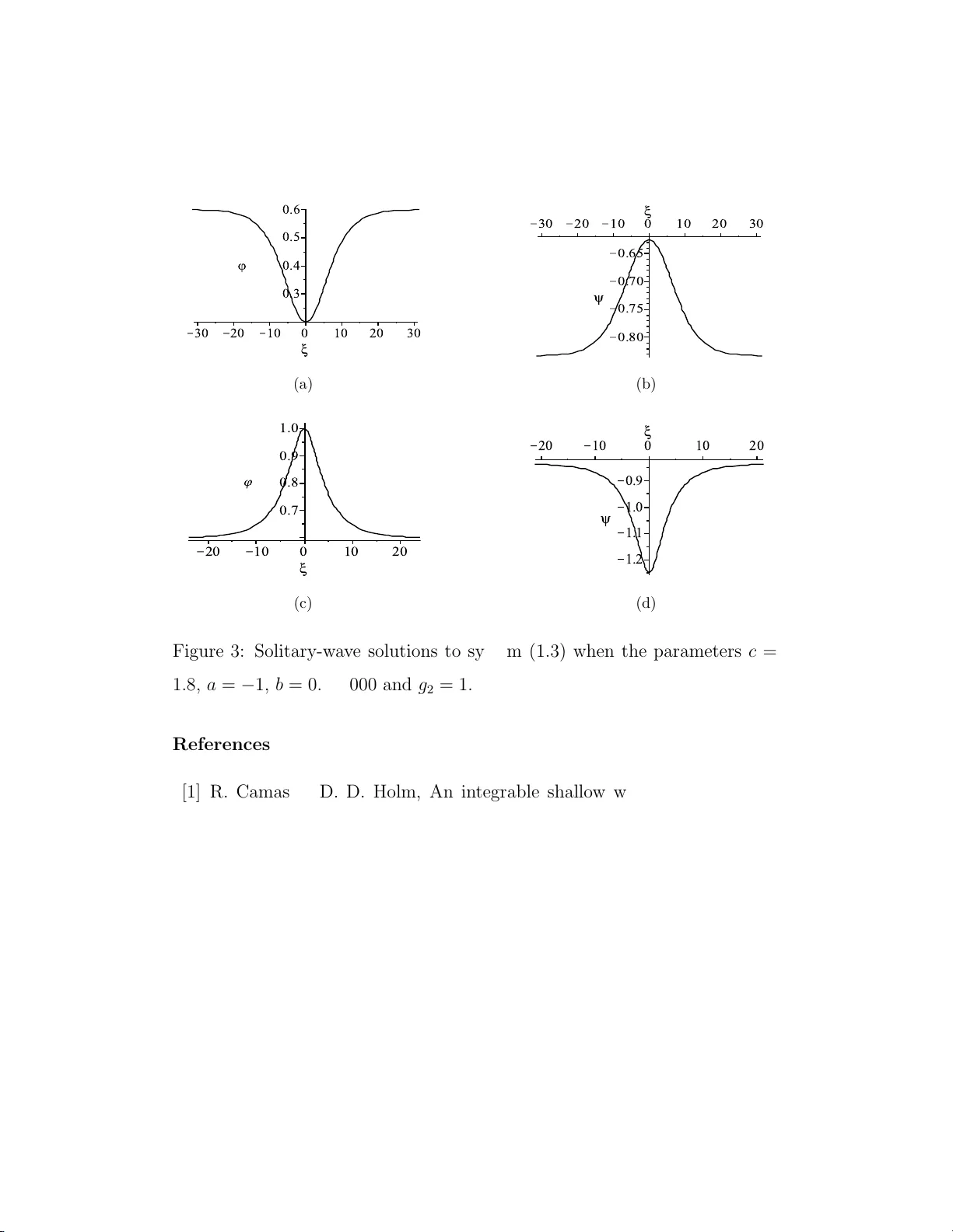
Solitary-wa v e solutions to a dual equation o f the Kaup-Boussinesq system Jiangb o Zhou ∗ , Lixin Tian , Xingh ua F an Nonline ar Scientific R ese ar ch Center, F a culty of Scienc e, Jiangsu University, Zhenjiang, Jiangsu 212013, China Abstract In this pap er, w e emplo y the bifurcation theory o f planar dynamical systems to inv estigate the trav elling-wa v e solutions to a d ual equ ation of the Kaup- Boussinesq system. The expressions for smo oth solitary-wa v e s olutions are obtained. Key wor ds: dual equation of the Kaup-Boussinesq system, solitary-wa v e solution, bif urcat io n metho d 2000 MSC: 35Q51 , 34C23, 3 7 G10, 35Q35 1. In tro duction Since the theory o f solito ns has very wide applications in fluid dynamics, nonlinear optics, bio che mistry , microbiolog y , ph ysics and many other fields, the study of soliton solutions to nonlinear part ia l differential equations has b ecome an increasingly imp o rtan t area of researc h [1]-[5]. It is kno wn that, solitons are the solitary w av es that retain their individualit y under in teraction and ev entually tra v el with their original shap es a nd sp eeds. Therefore, to ∗ Corresp o nding author. T el: + 86-5 11-88 969336, F ax : +8 6-51 1-889 69336 Email addr ess: zho ujian gbo@y ahoo.cn (Jiangb o Zhou) Novemb er 9, 2018 in v estigate the soliton solutions, one must firstly obtain the solitary- wa ve solutions. Man y efforts hav e b een denoted t o seeking solitary-w av e solutions to nonlinear partial differen tial equations (see, e.g., [6]-[13]). Recen tly , Guha [14] studied the dual counter part of the f ollo wing Kaup- Boussinesq system [15],    u t = v xxx + 2( uv ) x , v t = u x + 2 v v x , (1.1) where u ( x, t ) denotes the height of the w a ter surface a b ov e a horizon tal b ot- tom and v ( x, t ) is related to t he ho r izontal v elo city field. Using momen t of inertia op erators metho d and the frozen Lie-P oisson structure, Guha deriv ed the dual counte r part of system (1.1) , that is    m t + ( mu + 1 2 u 2 x + u 2 + 2 uv ) x = 0 , p t + ( pu ) x = 0 , (1.2) where m = u xx + µu + λv , p = λu + v . System (1 .2) is a t w o comp onent in tegrable system [14]. When µ = λ = 0 , it b ecomes    u xxt + ( uu xx + 1 2 u 2 x + u 2 + 2 uv ) x = 0 , v t + ( uv ) x = 0 . (1.3) V arious asp ects o f the Kaup-Boussinesq system (1.1) ha v e b een studied. F or instance , Smirno v [16] obta ined real finite gap r egula r solutions to sy stem (1.1), and Boriso v et al. [17] applied the proliferation sc heme to system (1.1). Also the closely related v arian t of system (1.1) hav e b een studied in tensiv ely (see [18]-[2 9]). How ev er, it seems that the dual equation o f system ( 1.1) has attracted little a t t en tion. 2 In this pap er, we use the bifurcation theory of planar dynamical systems (see [3 0]-[3 3 ]) to inv estigate the trav elling-w av e solutions to system (1.3) and obtain analytic expressions for its smo oth solitary-w av e solutions. T o the b est of our knowledge, the solitary-w av e solutions to system (1.3) ha v e not b een rep orted in the literature. The bifurcatio n metho d was first used by Li and Liu [34] to obtain smo oth and non-smo oth tr a v elling-w av e solutions to a nonlinearly disp ersiv e equation and w as later employ ed b y many authors to deriv e a v ariety of trav elling-w av e solutions to a la rge num b er of nonlinear partial differential equations [35]-[42]. The remainder of the pap er is org anized as follo ws. In Section 2, using the tra v elling-wa v e ansatz, w e transform system (1.3) into a plana r dynamical system and then discuss bifurcations of phase p o rtraits of this system. In Section 3, we obtain the expressions f o r smo oth solitary-w av e solutions to system (1.3) . A short conclusion is giv en in Section 4. 2. Bifurcation analysis Let ξ = x − ct , where c is the wa ve sp eed. By using the trav elling-w av e ansatz u ( x, t ) = ϕ ( x − ct ) = ϕ ( ξ ), v ( x, t ) = ψ ( x − ct ) = ψ ( ξ ), we reduce system (1.3) to the follo wing o r dina r y differential equations:    − cϕ ′′′ + ( ϕϕ ′′ + 1 2 ϕ ′ 2 + ϕ 2 + 2 ϕψ ) ′ = 0 , − cψ ′ + ( ϕψ ) ′ = 0 . (2.1) In tegrating (2.1) once with resp ect to ξ , we hav e    − cϕ ′′ + ϕϕ ′′ + 1 2 ϕ ′ 2 + ϕ 2 + 2 ϕψ = g 1 , − cψ + ϕψ = g 2 , (2.2) 3 where g 1 , g 2 are tw o inte gral constants. F rom the second equation in system (2.2), w e obtain ψ = g 2 ϕ − c . (2.3) Substituting (2.3) in to the first equation in system (2.2) yields ϕ ′′ = ( ϕ − c )( g 1 − 1 2 ϕ ′ 2 − ϕ 2 ) − 2 g 2 ϕ ( ϕ − c ) 2 . (2.4) Let ϕ ′ = √ 2 2 y , then w e get the followin g planar dynamical system:      dϕ dξ = √ 2 2 y , dy dξ = √ 2(( ϕ − c )( g 1 − 1 2 y 2 − ϕ 2 ) − 2 g 2 ϕ ) ( ϕ − c ) 2 . (2.5) This is a planar Hamiltonian system with Hamiltonian function H ( ϕ, y ) = ϕ 4 − 4 c 3 ϕ 3 + (4 g 2 − 2 g 1 ) ϕ 2 + 4 cg 1 ϕ + ( ϕ − c ) 2 y 2 = h, (2.6) where h is a constant. Note that (2.5) has a singular line ϕ = c . T o a v oid the line temp orarily w e mak e transformation dξ = √ 2 2 ( ϕ − c ) 2 dζ . Under this transformation, Eq.(2.5) b ecomes    dϕ dζ = 1 2 ( ϕ − c ) 2 y , dy dζ = ( ϕ − c )( g 1 − 1 2 y 2 − ϕ 2 ) − 2 g 2 ϕ. (2.7) System (2.5) and system (2 .7) hav e the same first in tegral as (2.6) . Con- sequen tly , system (2.7 ) has the same top ological phase p ortraits as system (2.5) except for the straig h t line ϕ = c . F or a fixed h , (2.6) determines a set of inv ariant curv es of syste m (2.7). As h is v aried, (2.6) determines differen t families of orbits of system (2.7) havin g 4 differen t dynamical b eha viors. Let M ( ϕ e , y e ) b e the co efficien t matrix of the linearized v ersion o f system (2.7) at t he equilibrium p o in t ( ϕ e , y e ), then M ( ϕ e , y e ) =   ( ϕ e − c ) y e 1 2 ( ϕ e − c ) 2 − 3 ϕ 2 e + 2 cϕ e + g 1 − 2 g 2 − 1 2 y 2 − ( ϕ e − c ) y e   (2.8) and at this equilibrium p oin t, w e hav e J ( ϕ e , y e ) = det M ( ϕ e , y e ) = − ( ϕ e − c ) 2 y 2 e + 1 2 ( ϕ e − c ) 2 (3 ϕ 2 e − 2 cϕ e − g 1 + 2 g 2 + 1 2 y 2 ) , (2.9) p ( ϕ e , y e ) = tra ce( M ( ϕ e , y e )) = 0 . (2.10) It is easy t o see that the equilibrium p oin t of system (2.7) is in the form of ( ϕ e , 0). At this equilibrium p oint, w e hav e J ( ϕ e , 0) = 1 2 ( ϕ e − c ) 2 (3 ϕ 2 e − 2 cϕ e − g 1 + 2 g 2 ). By using the bifurcation theory of planar dynamical system, w e kno w that if J ( ϕ e , 0) > 0 (or < 0), then the equilibrium ( ϕ e , 0) is a cen ter (or saddle) p o in t; if J ( ϕ e , 0) = 0, and the Poincar ´ e index of the equilibrium p oint is 0, then it is a cusp. Usually , a solitary-w a v e solution t o system (1.3) corresp o nds to a ho mo - clinic orbit of system (2.7). Therefore, to obtain solitary-wa v e solutions to system (1.3), w e need only to seek homo clinic orbits o f system (2.7) and so only the saddle p oints are of interes t. Firstly , w e need to lo ok for the po ssible zeros of the f unction f ( ϕ ) = − ϕ 3 + cϕ 2 + aϕ + b , (2.11) where a = g 1 − 2 g 2 , b = − cg 1 . In or der to find a ll p ossible zeros of f ( ϕ ), w e set f ′ ( ϕ ) = − 3 ϕ 2 + 2 cϕ + a = 0 . (2.12) 5 When ∆ = 4 c 2 + 12 a > 0, we find t w o real ro ots to Eq.(2.12) as follows : ϕ ∗ 1 = 1 3 ( c − √ c 2 + 3 a ) , (2.13) ϕ ∗ 2 = 1 3 ( c + √ c 2 + 3 a ) , (2.14) with ϕ ∗ 1 < ϕ ∗ 2 . When ∆ = 4 c 2 + 12 a ≤ 0, the inequalit y f ′ ( ϕ ) ≤ 0 holds. In this case, if ( ϕ e , 0) is an equilibrium p oin t of system (2.7), then it is a cen ter p oint (o r a cusp) b ecause J ( ϕ e , 0) = − 1 2 ( ϕ e − c ) 2 f ′ ( ϕ e ) ≥ 0. Therefore, in the fo llowing, w e alw a ys supp ose ∆ = 4 c 2 + 12 a > 0. Substitute (2.13) a nd (2.1 4) in to (2.11), resp ectiv ely , we get f 1 = f ( ϕ ∗ 1 ) = 2 c 3 27 − 2 c 2 27 √ c 2 + 3 a − 2 a 9 √ c 2 + 3 a + ac 3 + b, (2.15) f 2 = f ( ϕ ∗ 2 ) = 2 c 3 27 + 2 c 2 27 √ c 2 + 3 a + 2 a 9 √ c 2 + 3 a + ac 3 + b, (2.16) with f 1 − f 2 = − 2 c 2 27 √ c 2 + 3 a ( c 2 + 3 a ) < 0 . (2.17) The equilibrium p oin ts of system (2.7) ha v e the following prop erties. Theorem 2.1. (1 ) If f 2 < 0 , then s ystem (2.7) has only one e quilibrium p oint, den ote d by ( ϕ 1 , 0)( ϕ 1 < ϕ ∗ 1 < ϕ ∗ 2 ) , which is a c enter p oint; (2) I f f 1 > 0 , then system (2.7) has only one e quilib rium p oint, den ote d by ( ϕ 2 , 0)( ϕ ∗ 1 < ϕ ∗ 2 < ϕ 2 ) , wh ich is a c enter p oint; (3) If f 1 = 0 , then system (2.7) has two e quilibrium p oints, denote d b y ( ϕ 3 , 0) , ( ϕ 4 , 0)( ϕ 3 = ϕ ∗ 1 < ϕ ∗ 2 < ϕ 4 ) . ( ϕ 3 , 0) is a c usp, while ( ϕ 4 , 0) is a c enter p oint; 6 (4) If f 2 = 0 , then system (2.7) has two e quilibrium p oints, denote d b y ( ϕ 5 , 0) , ( ϕ 6 , 0)( ϕ 5 < ϕ ∗ 1 < ϕ ∗ 2 = ϕ 6 ) . ( ϕ 5 , 0) is a c enter p oint, while ( ϕ 6 , 0) is a cusp; (5) If f 1 < 0 , f 2 > 0 , then system (2.7) has t hr e e e quilibrium p oints, denote d by ( ϕ 7 , 0) , ( ϕ 8 , 0) and ( ϕ 9 , 0)( ϕ 7 < ϕ ∗ 1 < ϕ 8 < ϕ ∗ 2 < ϕ 9 ) . ( ϕ 7 , 0) and ( ϕ 9 , 0) ar e two c enter p o ints, wh ile ( ϕ 8 , 0) is a sadd le p oint. In this pap er, we only consider the case c > 0 b ecause in the case c < 0 w e will get analogous result. I n order to giv e the details of t he bif urcat io n, w e fix t he para meter a = − 1. Thus , we obtain the follo wing t w o bifurcation curv es of system (2.7). L 1 : b = − 2 c 3 27 + 2 c 2 27 √ c 2 − 3 − 2 9 √ c 2 − 3 + c 3 , L 2 : b = − 2 c 3 27 − 2 c 2 27 √ c 2 − 3 + 2 9 √ c 2 − 3 + c 3 . The ab ov e bifurcation curv es divide the parameter space in to three re- gions (see Fig. 1) in whic h differen t phase p ortraits exist. By theorem 2.1 , w e can see that o nly in regions (I I), can system (2.7) has saddle p oints. See Fig. 2 for an example of t he corresp onding phase p o r t raits. 3. Solitary-w a v e solutions to system (1.3) F rom the discussions in Section 2, we can see that, when the para meters a = − 1, ( b, c ) ∈ (I I), system (2.7) has infinite man y saddle points. So there a re infinite ma ny ho mo clinic orbits and system (1.3) has infinite man y solitary-w a v e solutions accordingly . 7 L 1 II I L 2 III c 2.0 2.5 3.0 3.5 4.0 4.5 b K 0.6 K 0.4 K 0.2 0.0 0.2 0.4 Figure 1: The bifurcation sets and bifurcation curv es of system (2.7) for the parameter c > √ 3. In order to obtain exact expressions for solitary-w a v e solutions, w e fix b = − 2 c 3 27 + c 3 . Case I : √ 3 < c < 3 In this case, there are tw o homo clinic orbits connecting with the saddle p oint ( c 3 , 0), see Fig. 2(a) for an example. The tw o homo clinic orbits of system (2.7) or (2.5) can b e expressed resp ectiv ely as y = ± ( ϕ − c 3 ) q − ϕ 2 + 2 c 3 ϕ + 5 c 2 9 − 2 ϕ − c for ϕ − ≤ ϕ ≤ c 3 , (3.1) y = ± ( ϕ − c 3 ) q − ϕ 2 + 2 c 3 ϕ + 5 c 2 9 − 2 ϕ − c for c 3 ≤ ϕ ≤ ϕ + , (3.2) where ϕ ± = 1 3 ( c ± √ 6 c 2 − 18). Substituting (3.1), (3 .2 ) in to the first equation of system (2.5), resp ec- tiv ely , and in tegrating alo ng the cor r esp onding homo clinic orbit, w e hav e Z ϕ ϕ − s − c ( s − c 3 ) q − s 2 + 2 c 3 s + 5 c 2 9 − 2 ds = √ 2 2 | ξ | , (3.3) 8 4 0.3 0.4 0.5 0.6 0.7 0.8 0.9 1.0 y K 0.08 K 0.06 K 0.04 K 0.02 0.00 0.02 0.04 0.06 0.08 (a) 4 K 1 1 2 y K 0.8 K 0.2 0.2 0.8 (b) Figure 2: The phase p or t raits of system (2.7) when the para meters c > √ 3, a = − 1 and b = − 2 c 3 27 + c 3 . (a) c = 1 . 8; (b) c = 4 . Z ϕ + ϕ s − c ( s − c 3 ) q − s 2 + 2 c 3 s + 5 c 2 9 − 2 ds = − √ 2 2 | ξ | , (3.4) It follows from (3.3), (3.4 ) that π 2 + arctan( α ( ϕ )) + 2 c √ 6 c 2 − 18 ln( β ( ϕ )) = √ 2 2 | ξ | , ϕ − ≤ ϕ ≤ c 3 , (3.5) and π 2 − arctan( α ( ϕ )) − 2 c √ 6 c 2 − 18 ln( − β ( ϕ )) = √ 2 2 | ξ | , c 3 ≤ ϕ ≤ ϕ + , (3.6) where α ( ϕ ) = 3 ϕ − c p − 9 ϕ 2 + 6 cϕ + 5 c 2 − 18 , (3.7) β ( ϕ ) = √ 6 c 2 − 18 + p − 9 ϕ 2 + 6 cϕ + 5 c 2 − 18 c − 3 ϕ . (3.8) Therefore, w e obta in tw o solitary-w av e solutions to system (1.3) in the 9 follo wing parametric forms:    ξ = ± √ 2( π 2 + arctan( α ( ϕ )) + 2 c √ 6 c 2 − 18 ln( β ( ϕ )) , ϕ = ϕ, ( ϕ − ≤ ϕ ≤ c 3 ) , (3.9)    ξ = ± √ 2( π 2 + arctan( α ( ϕ )) + 2 c √ 6 c 2 − 18 ln( β ( ϕ )) , ψ = g 2 ϕ − c , ( ϕ − ≤ ϕ ≤ c 3 ) , (3 .1 0) and    ξ = ± √ 2( π 2 − arctan( α ( ϕ )) − 2 c √ 6 c 2 − 18 ln( − β ( ϕ )) , ϕ = ϕ, ( c 3 ≤ ϕ ≤ ϕ + ) , (3 .1 1)    ξ = ± √ 2( π 2 − arctan( α ( ϕ )) − 2 c √ 6 c 2 − 18 ln( − β ( ϕ )) , ψ = g 2 ϕ − c , ( c 3 ≤ ϕ ≤ ϕ + ) . (3 .1 2) No w we ta ke a set of data and employ Maple to display the graphs of the ab ov e obtained solitar y-w a v e solutions in Fig. 3 . Case I I: c ≥ 3 In this case, there is one homo clinic o r bit connecting with t he saddle p oint ( c 3 , 0), see Fig. 2 ( b) for an example. Similar to the Case I, we can obta in a solitary-w av e solution to system (1.3), g iven as (3 .9), (3.10). A t ypical suc h solution is shown in Fig. 4. 4. Conclusion In summary , b y using the bifurcatio n metho d, w e obta in ana lytic ex- pressions f or smo oth solita ry-w a v e solutions to a dual equation of the Kaup- Boussinesq system (1 .3). The results of this pap er suggest that, in addition to solving many single-comp o nen t par t ia l differen tial equations, the bifurcation metho d can b e used to obtain t r av elling-wa ve solutions of tw o- comp onen t systems . 10 x K 30 K 20 K 10 0 10 20 30 4 0.3 0.4 0.5 0.6 (a) x K 30 K 20 K 10 0 10 20 30 y K 0.80 K 0.75 K 0.70 K 0.65 (b) x K 20 K 10 0 10 20 4 0.7 0.8 0.9 1.0 (c) x K 20 K 10 0 10 20 y K 1.2 K 1.1 K 1.0 K 0.9 (d) Figure 3: So lit a ry-w a v e solutions t o system (1.3) when the par a meters c = 1 . 8, a = − 1, b = 0 . 168000 a nd g 2 = 1. References [1] R. Camassa, D. D . Ho lm, An integrable shallow w ater equation with p eak ed solitons, Ph ys. Rev. Lett. 7 1 (19 9 3) 16 6 1-1664 . [2] A. Constan tin, W. Strauss, Stabilit y of the Camassa-Holm solitons, J. Nonlinear Sci. 12 (20 0 2) 415-4 22. [3] R. S. Johnson, On solutions of the Camassa-Holm equation, Pro c. Roy . So c. London A 459 (2003) 1687- 1 708. 11 x K 10 K 5 5 10 4 K 1.5 K 1.0 K 0.5 0.5 1.0 1.5 (a) x K 10 K 5 0 5 10 y K 0.34 K 0.30 K 0.24 K 0.20 (b) Figure 4: Solitary-w av e solution to system (1.3) when the para meters c = 4, a = − 1, b = − 3 . 40740 7 and g 2 = 1. [4] A. Park er, W a v e dynamics fo r p eak ed solitons of the Camassa-Holm equation, Chaos Solit ons F ractals 35 (2008) 220-37. [5] A. P ark er, Cusp ed solitons of the Camassa-Holm equation. I I. Binary cuspo nsoliton inte ractions, Chaos Solitons F ractals 41 (2009) 1531-154 9. [6] V. O. V akhnenk o, E. J. Park es, P erio dic and solitary-wa ve solutions of the D egasp eris-Pro cesi equation, Chaos Solitons F ractals 20 (2004) 1059-10 73. [7] J. Lenells, T rav eling w av e solutions of the D egasp eris-Pro cesi equation, J. Math. Anal. Appl. 306 ( 2 005) 72- 82. [8] J. H. He, X. H. W u, Construction of solitary solution a nd compacton- lik e solution b y v aria t ional iteration metho d, Chaos Solitons F ractals 29 (2006) 108-113 . [9] A. P ark er, Cusped solito ns of the Camassa-Holm equation. I. Cuspo n 12 solitary w av e and antipeak on limit, Chaos Solito ns F ractals 34 (20 0 7) 730-739 . [10] E. J. P ark es, Some p erio dic and solitary trav elling-wa v e solutions of the short-pulse equation, Chaos So lit ons F ractals 36 (2008) 154-159. [11] I. Mustafa, New solitary w a v e solutions with compact supp ort and Ja- cobi elliptic function solutions fo r the nonlinearly disp ersiv e Boussinesq equations, Chaos Solitons F ractals 37 (2008) 79 2-798. [12] F. Khanib, S. Hamedi-Nezhadc, M. T. Darvishia, Sang - W an Ryua, New solitary w av e and p erio dic solutions of the foam drainag e equation using the Exp-function metho d, Nonlinear Anal. R W A 1 0 (2009 ) 1904-191 1. [13] S. Abbasbandy , Solitary w av e solutions to the mo dified form of Camassa- Holm equation b y means of the ho mo t op y analysis metho d, Chaos Soli- tons F ractals 39 (2009 ) 428-43 5 . [14] P . Guha, Geo desic flo w on extended b ott-virasoro group and generalized t w o-comp o nen t p eak on type dual systems, Rev. Math. Ph ys. 20 (2008) 1191-12 08. [15] D. J. Kaup, Finding eigen v alue pro blems for solving nonlinear ev olution equations, Progr. Theoret. Ph ys. 5 4 (197 5) 72-78 . [16] A. O. Smirno v, Real finite ga p regular solutions of the Kaup-Boussinesq equation, Theoret. Math. Ph ys. 6 6 (1986 ) 19-31. [17] A. B. Borisov , M. P . P avlo v, S. A. Zyk o v, Proliferat io n sc heme for Kaup- Boussinesq system, Phy sica D (1 5 2/153) (2001) 104- 1 09. 13 [18] A. M. Kamchatno v, R. A. Kraenk el, B. A. Umaro v, Asymptotic soliton train solutions of Ka up-Boussinesq equations, W a v e Motion 3 8 (200 3 ) 355-365 . [19] G. A. El, R. H. J. Grimsha w, M. V. P avlo v, In tegrable shallow -water equations and undular b ores, Stud. Appl. Math. 106 (20 01) 15 7-186. [20] V. B. Matve ev, M. I. Y av or, Almost p erio dical solutions of nonlinear hy- dro dynamic equation of Kaup, Ann. Inst. H. P oincar, Sect. A 31 (1979) 25-41. [21] E. Y om ba, The extended F an’s sub-equation metho d and its application to KdV-MKdV, BKK and v arian t Boussinesq equations, Phy s. Lett. A 336 (2 005) 463-476. [22] J. B. Li, Z. R. L iu, T rav elling w av e solutions for a class of nonlinear disp ersiv e equations, Chin. Ann. Math. Ser. B 23 (2002) 397- 418 [23] M. L. W a ng , Solitar y w av e solutions of v ariant Boussinesq equations, Ph ys. Lett. A 199 (1995) 169-1 7 2 [24] Z. Y. Y an, H. Q. Zhang, New explic it and exact tra v elling w av e solutions for a system o f v arian t Boussinesq equations in ma t hematical ph ysics, Ph ys. Lett. A 252 (1999) 291-2 9 6. [25] D. Z. L ¨ u, Jacobi elliptic function solutions fo r tw o v ariant Boussinesq equations, Chaos Solitons F ractals 24 (2005) 13 73-1385 . [26] J. F. Zhang , Multi-solitary wa v e solutions for v aria nt Boussinesq equa- tions and Kup ershmidt equations, Appl. Math. Mec h. 21 (200 0) 193-198 14 [27] Y. B. Y uan, D . M. Pu, S. M. Li, Bifurcations of trav elling w av e solutio ns in v a rian t Boussinesq equations, Appl. Math. Mec h. 27 (2006) 811-82 2 . [28] E. G. F an, Tw o new applications of the homog eneous balance metho d, Ph ys. Lett. A 265 (1998) 353-3 5 7. [29] E. F an, Y. Ho n, A series of tra v eling w av e solutions fo r tw o v ariant Boussinesq equations in shallo w w a ter w a v es, Chaos Solitons F ractals 15 (20 03) 5 5 9-566. [30] D. Luo, et al., Bifurcation Theory and Metho ds of D ynamical Systems, W orld Scien tific Publishing Co., London, 1997 . [31] S. N. Chow , J. K. Hale, Metho d of Bifurcatio n Theory , Springer, New Y ork, 1 981. [32] J. Guck enheimer, P . Holmes, Nonlinear Oscillations, Dynamical Systems and Bif urcation of V ector Fields, Springer, New Y ork, 1983 . [33] L. Perk o, Differen tial Equations and Dynamical Systems, Springer, New Y ork, 1 991. [34] J. B. Li, Z . R. Liu, Smo oth and non-smo oth trav eling wa v es in a non- linearly disp ersiv e equation, Appl. Math. Mo del. 25 (20 00) 41-5 6 . [35] T. F. Qian, M. Y. T ang, P eak ons and p erio dic cus p w a v e in a generalized Camassa-Holm equation, Chao s Solitons F ractals 12 (2001) 134 7-1360. [36] J. W. Shen, W. Xu, Bifurcations of smo oth a nd non-smo oth trav eling w a v e solutions in the g eneralized Camassa-Holm equation, Chaos Soli- tons F ractals 26 (2005 ) 1149-1 1 62. 15 [37] L. J. Z hang, L. Q. Chen, X. W. Huo, P eak ons and p erio dic cusp w av e solutions in a generalized Camassa-Holm equation, Chaos Solitons F rac- tals 3 0 (200 6) 12 38-1249 . [38] Z. R. Liu, Z . R. Ouy ang, A note on solitary w av es for mo dified f o rms of Camassa-Holm and Degasp eris-Pro cesi equations, Ph ys. Lett. A 366 (2007) 377-381 . [39] J. B. Zhou, L. X. Tian, Solito n solution of the osmosis K (2 , 2) equation, Ph ys. Lett. A 372 (2008) 6232- 6 234. [40] A. Y. Chen, W. T. Huang , S. Q. T ang, Bifurcations of trav elling w a v e solutions fo r the Gilson-Pic k ering equation, Nonlinear Anal. R W A 10 (2009) 2659-26 65. [41] J. B. Z hou, L. X. Tian, Solitons, p eak ons and p erio dic cusp w a v e solu- tions for the F or nberg- Whitham equation, Nonlinear Anal. R W A (200 9 ), in press (doi:10 .1 016/j.nonrwa.2008.11.014). [42] J. B. Zhou, L. X. Tian, X. H. F an, Soliton, kink and a ntikink solutions of a 2-comp onent of the D egasp eris-Pro cesi equation, Nonlinear Anal. R W A (2009), in press (doi:1 0.1016/j .no nrw a.2009.08 .0 09). 16