From real fields to complex Calogero particles
We provide a novel procedure to obtain complex PT-symmetric multi-particle Calogero systems. Instead of extending or deforming real Calogero systems, we explore here the possibilities for complex systems to arise from real nonlinear field equations. …
Authors: Paulo E. G. Assis, Andreas Fring
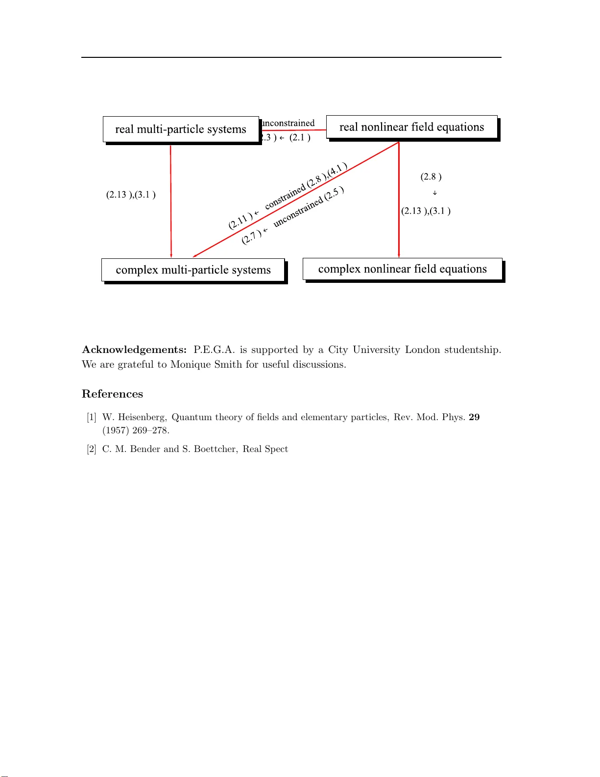
F r om r e al fields to c omplex Calo g er o p articles F rom real fields to complex Calogero pa rticl es P aulo E. G. Assis and Andreas Fring Centr e for Mathema tic al Scienc e, City University L ondon, Northampton Squar e, L ondon EC 1V 0HB, UK E-mail: Paulo.Gonc alves-de-Assis.1@city.ac.uk, A.F ring@city.ac.uk Abstract: W e provide a novel procedure to obta in complex P T -symmetric m ulti-particle Caloger o systems. Instead of extending or deforming re a l Calogero systems, we explore here the poss ibilities for complex systems to arise from r eal nonlinea r field equations. W e exemplify this pro ce dure for the Boussine s q equa tion and demonstrate how singular ities in real v alued wav e solutions can b e interpreted as N complex particles scattering amongst each other. W e analyze this phenomenon in more deta il for the tw o and three particle case. Particular attention is paid to the implemention o f P T - symmetry for the complex m ulti-particle sy stems. New complex P T -symmetric Calog ero sys tems together with their classical solutions are derived. 1. In t ro duction The analytic con tin uation of real p h ysical systems int o the complex p lane is a principle whic h h as turned out to b e very fruitful, s ince many new features can b e revea led in this manner w h ic h migh t otherwise b e und etected. A famous and already classical example, prop osed more than half a cen tury ago, is fo r i nstance Heisenberg’s programme of t he analytic S-matrix [1]. Here our main concern will b e complex m u lti-particle Calog ero systems, in particular th ose exhibiting P T -symmetry [2]. Quant um systems are said to b e P T -symmetric when they are in v arian t under si- m ultaneous parit y P and time rev ersal T transformations. When the Hamiltonian, n ot necessarily Hermitian, exhibits this symmetry , i.e. [ H , P T ] = 0, and moreo v er when all w a ve-functions are also inv arian t u nder suc h an op eration this prop ert y is referr ed to as unbrok en P T -symmetry . The virtue of this feature is that it is a sufficien t prop ert y to guaran tee the sp ectrum of the Hamiltonian H to b e real. The u nderlying mec h anisms resp onsib le for th is are by n ow well und ersto o d [3, 4 , 5 , 6] and ma y b e formulated al- ternativ ely in terms of pseudo/quasi-Hermiticit y; for defin itions see for instance [7] and references therein. There are tw o fund amen tally differen t p ossibilities to view complex systems: One ma y either r egard the complexified v ersion ju st as a broader fr amework, as in the sp irit of the F r om r e al fields to c omplex Calo g er o p articles analytic S-matrix, and restrict to the real case in order to d escrib e the u nderlying p h ysics or alternativ ely one ma y try to giv e a direct ph ysical meaning to the complex mo dels. With th e latter motiv ation in min d complex P T -symmetric Calogero systems h a ve b een in tro duced and studied recen tly [8 , 9, 10, 11, 12]. The h op e for a direct p h ysical in terpretation stems from the fact that unbrok en P T -symmetry w ill guarant ee their eigen- sp ectra to b e real an d allo ws for a consistent quantum mec h anical d escription, i.e. s u c h systems constitute we ll d efined q u an tum sys tems wh ic h h a ve b een o v erlo ok ed u p to n o w. Nonetheless, so far an y suc h prop osal lac ks a d irect ph ysical m eanin g and the complexi- fications are generally introd u ced in a rather ad ho c mann er. Here our main purp ose is to demonstrate that v arious complex Calogero mo dels app ear rather naturally fr om r e al v alued nonlinear field equations and thus w e p ro vide a well defined physic al origin for th ese systems. The sol utions for th e real Calogero systems were foun d in the rev erse order w hen compared to the usu al wa y pr ogress is made, i.e. the qu an tum theory w as solve d b efore the classical one. Calogero solv ed firs t the quan tized one-dimensional thr ee-b o dy p roblem with pairwise inv erse square inte raction [13] and su bsequentl y constructed the groun d state of the N -b o d y generalization [14] describ ed by the Hamiltonian H C = N X i =1 p 2 i 2 + 1 2 N X i 6 = j g ( x i − x j ) 2 , (1.1) with g ∈ R b eing the coupling constan t. Ma rc hioro [15, 16] inv estigated thereafter the classical analogue of these mo dels obtaining a solution to whic h w e will app eal b elo w . The in tegrabilit y of these classical counterparts was established later b y Moser [17], using a Lax pair consisting of matrices L, M , with en tries L ij = p i δ ij + ı √ g x i − x j (1 − δ ij ) , (1.2) M ij = N X k 6 = i ı √ g ( x i − x k ) 2 δ ij − ı √ g ( x i − x j ) 2 (1 − δ ij ) , (1.3) constructed in suc h a manner that the Lax equation dL dt + [ M , L ] = 0 (1.4) b ecomes equiv alen t to the Caloge ro equations of motion, ¨ x i = N X j 6 = i 2 g ( x i − x j ) 3 . (1.5) W e use the notatio n ı ≡ √ − 1 throughout the man uscript and abbreviate time deriv ativ es as u sual by dx i /dt = ˙ x i and d 2 x i /dt 2 = ¨ x i . In tegrabilit y follo ws in th e standard fashion b y noting that all quanti ties of the for I n = tr( L n ) /n are integ rals of motion and conserved in time b y constru ction. – 2 – F r om r e al fields to c omplex Calo g er o p articles Calogero systems ha ve b ecome v er y imp ortant in theoretical p h ysics, ha vin g b een explored i n v arious cont exts ranging from co ndensed matte r ph ys ics to co smology , e.g. [18, 19, 20]. The main focu s of our interest h ere are th e complex extensions whic h ha ve b een studied recen tly in connection with P T -symmetric mo dels [8, 9, 10 , 11, 12]. The idea of exploiting P T -symmetry in order to obtain mo dels with real en ergies can b e adapted to classical systems as well and h as b een used to formulate v arious complex extensions of nonlinear wa ve equations, such as the Korteweg -de V ries (KdV) and Burgers equations [21, 22, 23, 24]. In the classical case the realit y of the energy is ensu red in an ev en simpler wa y , as in that case th e P T -symmetry of the Hamiltonian is sufficien t. Remark ably these systems allo w for the existence of solitons and compacton solutions [25, 26]. Here we sh all explore P T -symmetry in a con text where the complex extensions or deformations do not need to b e imp osed artificially , bu t instead we inv estigate wh ether this symmetry is already naturally presen t in the system, alb eit hidden. T o ac hiev e this goal we exploit the fact that nonlinear equations, suc h as Benjamin-Ono and Boussinesq, can b e asso ciated to Calogero particle systems. W e explore these connections and are then naturally led to complex P T -symmetric Calogero systems. In th e next section w e shall d emonstrate ho w a complex one-dimensional P T -symmetric Calogero system is emb edded in a real solitonic solution of the Benjamin-Ono w a v e equa- tion and ho w constrained P T -symm etric Calogero particles emerge from real solutions of the Boussinesq equation. Th er eafter we constr u ct the explicit solution of the three-particle configuration with the aforemen tioned constraint and sho w that th e resulting motion, un- lik e in the u nconstrained situation, c annot b e restricted to the r eal line. W e shall also establish that a sub class of this constrained Calogero motion is related to the p oles in the solution of differen t nonlinear K dV-lik e differen tial equation. The relation of these com- plex particles with pr eviously obtained P T -sym metric complex extensions of the Calogero mo del [27] is discussed in section 5, where w e demonstrate that they are differen t from those prop osed here. Ou r conclusions are drawn in sectio n 6. 2. P oles of nonlinear wa ves as interacting particles The assu m ption of rational real v alued f unctions as m ulti-soliton solutions of nonlinear w a ve equations was studied more than three decades ago b y v arious authors, see e.g. [28]. W e tak e some of these findings as a setting for the problem at hand. I n order to illustrate the key idea we presen t what is p robably the simp lest scenario in w h ic h corpu scular ob jects emerge as p oles of nonlin ear wa v es, namely in the Bur gers equation u t + αu xx + β ( u 2 ) x = 0 . (2.1) Assuming that this equation admits rational solutions of the form u ( x, t ) = 2 α β N X i =1 1 x − x i ( t ) , (2.2) – 3 – F r om r e al fields to c omplex Calo g er o p articles it is straigh tforward to see that surp risingly the N p oles in teract with eac h other through a Coulom b ic inv erse squ are force ¨ x i ( t ) = − 2 α N X j 6 = i 1 [ x i ( t ) − x j ( t )] 2 . (2.3) This p ole structur e survive s ev en after making mo difications in th e ansatz for the w a v e equation, although the nature of the interac tion ma y c h ange. By acting on the second deriv ativ e in Burgers equation w ith a Hilb ert transf orm ˆ H u ( x ) = 1 π P V Z + ∞ −∞ dz u ( z ) z − x , (2.4) w e obtain the Benjamin -Ono equ ation [29, 30] u t + α ˆ H u xx + β ( u 2 ) x = 0 . (2.5) As shown in [31], the ansatz prop osed for the equ ation ab ov e whic h will allo w for similar conclusions has a slight ly different form, u ( x, t ) = α β N X k =1 ı x − z k ( t ) − ı x − z ∗ k ( t ) (2.6) b eing, ho w ev er, s till a real v alued solution w ith the only restriction that the complex p oles satisfy complex C alogero equations of motion ¨ z k ( t ) = 8 α 2 N X k 6 = j 1 ( z k ( t ) − z j ( t )) 3 . (2.7) Note that there is a difference in the p o wer la w s app earing in (2.3) and (2.7), but more imp ortan tly that equation (2.2) h as real p oles, wh ereas (2.6) has complex ones. W e stress once more that the field u ( x, t ) is real in b oth cases. Hence, this viewp oin t provides a non trivial mec h an ism which leads to particle systems d efi ned in the complex plane. In teresting observ ations of this k in d can b e made for other nonlin ear equations as wel l, but not alw a ys will the ansatz wo rk directly , that is without an y further requ ir emen ts as in the previous cases. In some situations additional conditions might b e necessary . Examples of nonlinear in tegrable wa v e equations for wh ic h such typ e of constrain ts o ccur are th e KdV and th e Boussinesq equations, u t + αu xx + β u 2 x = 0 and u tt + αu xx + β u 2 − γ u xx = 0 , (2.8) resp ectiv ely . F or b oth of these equations one can ha ve “ N -soliton” s olutions 1 of the form u ( x, t ) = − 6 α β N X k =1 1 ( x − x k ( t )) 2 , (2.9) 1 Soliton is to b e understo od here in a v ery lo ose sense in analogy to the Pai nlev´ e t yp e ideology of indistructable p oles. In the strict sense not all solution p ossess the N -soliton solution c haracteristic, that is moving with a preserved shap e and regaining it after scattering th ough each oth er. – 4 – F r om r e al fields to c omplex Calo g er o p articles as long as in eac h case tw o sets of constrain ts are satisfied ˙ x k ( t ) = − 12 α N X j 6 = k ( x k ( t ) − x j ( t )) − 2 , 0 = N X j 6 = k ( x k ( t ) − x j ( t )) − 3 , (2.10) and ¨ x k ( t ) = − 24 α N X j 6 = k ( x k ( t ) − x j ( t )) − 3 , ˙ x k ( t ) 2 = 12 α N X j 6 = k ( x k ( t ) − x j ( t )) − 2 + γ , (2.1 1) resp ectiv ely . Naturally these constrain ts might b e incompatible or admit n o solution at all, in whic h case (2.9) w ould of cours e not constitute a solution f or th e wa v e equ ations (2.8). Notice that if the x k ( t ) are real or come in complex conjugate p airs the solution (2.9) for the corresp onding w av e equ ations is still real. Airault, McKean and Moser provi ded a general criterium, whic h allo ws us to view these equations fr om an en tirely different p ersp ectiv e, namely to r egard them as constrained m ulti-particle systems [28]: Given a multi-p article Hamiltonian H ( x 1 , ..., x N , ˙ x 1 , ..., ˙ x N ) with flo w x i = ∂ H /∂ ˙ x i and ˙ x i = − ∂ H /∂ x i to gether with c onserve d char ges I n in involution with H , i.e . vanishing Poisson br ackets { H , I n } = 0 , then the lo cus of g r ad ( I n ) = 0 i s invariant with r esp e ct to time evolution. Thus it is p ermitte d to r estrict the flow to th at lo cus pr ovide d it is not empty. T aking the Hamiltonian to b e the Calogero Hamiltonian H C it is w ell kn own that one ma y construct the corresp onding conserved q u an tities from the Calogero Lax op erator (1.2) as mentioned from I n = tr( L n ) /n . The fi rst of these charge s is just the total momen tum, the next is the Hamltonian follo wed b y n on trivial ones I 1 = N X i =1 p i , I 2 = H C ( g ) , I 3 = 1 3 N X i =1 p 3 i + g N X i 6 = j p i + p j ( x i − x j ) 2 , . . . (2.12) According to the ab o v e men tioned criterium w e ma y therefore c onsider an I 3 -flo w restricted to the lo cu s defined by grad( I 2 ) = 0 or an I 2 -flo w sub ject to the c onstrain t grad( I 3 − γ I 1 ) = 0. Remark ably it turns out that the former viewp oin t corresp ond s exactly to the set of equations (2.10), whereas the latter to (2.11) wh en w e ident ify the coup ling constan t as g = − 12 α . Th us th e solutions of the Boussinesq equation are related to the constrained Calogero Hamiltonian flo w, whereas the KdV soliton solutions arise from an I 3 -flo w sub ject to constrainin g equations d eriv ed from the Calogero Hamiltonian. As our mai n focus is on the Calogero Ha miltonian flo w a nd its p ossible complexi- fications we shall concent rate on p ossible solutions of the systems (2.11) and inv estigate whether these t yp e of equations allo w f or non trivial solutions or whether they are empt y . It will b e instru ctiv e to commence by lo oking first at the unconstrained system. Th e classical solutions of a tw o-particle Calogero problem are give n by x 1 , 2 ( t ) = 2 R ( t ) ± r g E + 4 E ( t − t 0 ) 2 , (2.13) – 5 – F r om r e al fields to c omplex Calo g er o p articles with E , t 0 b eing initial conditions and ˙ R ( t ) = 0 the cent re of mass v elocity . Relaxing this condition by allo wing b o osts will only shifts the energy scale since the total momen tum is conserv ed. Dep ending therefore on the initial conditions we ma y ha v e either real or complex solutions. The thr ee p article m o del, i.e. taking N = 3 in (1.1), is slightly more complicated. Marc hioro [15] foun d the general solution by expressing the dynamical v ariables in terms of Jacobi relativ e co ordinates R , X , Y in p olar form via the transformations R ( t ) = ( x 1 ( t ) + x 2 ( t ) + x 3 ( t )) / 3, X ( t ) = r ( t ) s in φ ( t ) = ( x 1 ( t ) − x 2 ( t )) / √ 2 and Y ( t ) = r ( t ) cos φ ( t ) = ( x 1 ( t )+ x 2 ( t ) − 2 x 3 ( t )) / √ 6. The v ariables ma y then b e separated and th e resulting equations are solv ed by x 1 , 2 ( t ) = R ( t ) + 1 √ 6 r ( t ) cos φ ( t ) ± 1 √ 2 r ( t ) sin φ ( t ) , (2.14) x 3 ( t ) = R ( t ) − 2 √ 6 r ( t ) cos φ ( t ) , (2.15) where R ( t ) = R 0 + t ˜ R 0 (2.16) r ( t ) = r B 2 E + 2 E ( t − t 0 ) 2 , (2.17) φ ( t ) = 1 3 cos − 1 ( ϕ 0 sin " sin − 1 ( ϕ 0 cos 3 φ 0 ) − 3 tan − 1 √ 2 E B ( t − t 0 ) !#) . (2.18) The solutions in v olv e 7 fr ee parameters: The total energy E , the angular momentum typ e constan t of motion B , the inte gration constan ts t 0 , φ 0 , R 0 , ˜ R 0 and the coupling constant g , with the abbreviation ϕ 0 = p 1 − 9 g / 2 B 2 . W e note that, dep ending on the choice of these parameters, b oth real and complex solutions are admissible, a feature wh ic h migh t not hold f or th e Calogero system restricted to an inv ariant subm an if old. Let us no w elab orate fu rther on the connection b et w een the fi eld equations and the particle system and restrict the general solution (2.14 )-(2.16) by switc hing on the additional constrain ts in (2.11) and subs equen tly study the effect on the soliton solutions of the nonlinear wa v e equation. Notice that the second constraint in (2.11) can b e viewe d as setting the d ifference b et ween the kin etic and p oten tial ener gy of eac h particle to a constant . Adding all of these equations we obtain H C = N γ / 2, whic h provides a direct in terpretation of the constan t γ in the Boussin esq equation as b eing p rop ortional to the total energy of the Calogero m o del. 3. The motion of Boussinesq singularities The tw o particle s y s tem, i.e. N = 2, is eviden tly the simplest I 2 -Calogero flo w constrained with grad( I 3 − γ I 1 ) = 0 as sp ecified in (2.11). The solution for this system w as already pro vided in [28], x 1 , 2 ( t ) = κ ± p γ ( t − ˜ κ ) 2 − 3 α/γ , (3.1) – 6 – F r om r e al fields to c omplex Calo g er o p articles with κ, ˜ κ tak en to b e r eal constan ts. In fact this solution is not v ery different from the unconstrained motion s ho wn in the previous section (2.13). The restricted one ma y b e obtained via a n id en tification b et ween th e co upling c onstan t a nd the paramet er in the Boussinesq equation as κ = 2 R ( t ), E = γ / 4, ˜ κ = t 0 and g = − 3 α/ 4. Th e tw o soliton solution for the Boussinesq equation (2.9) then acquires th e form u ( x, t ) = − 12 α β γ γ ( x − κ ) 2 + γ 2 ( t − ˜ κ ) 2 − 3 α [ γ ( x − κ ) 2 − γ 2 ( t − ˜ κ ) 2 + 3 α ] 2 , (3.2) whic h, in prin ciple, is still real-v alued when kee ping the constan ts to b e real. When in- sp ecting (3.2) it is easy to see that the tw o singularities rep el eac h other on the x -axis as time ev olv es, thus mimic king a repu lsiv e scattering pro cess. Ho w ev er , we m ay c h ange the o v erall b eh aviour su b stan tially when we allo w the inte gration constan ts to b e complex, suc h that the sin gularities b ecome regularized. In th at case w e observ e a t ypical so li- tonic scattering b eha viour, i.e. tw o w a ve p ac ket s keeping their o veral l sh ap e while evolving in time and w h en passing though eac h other r egaining their sh ap e when the scattering pro cess is finish ed , alb eit with complex amp litude. A sp ecial typ e of complexification o c- curs when we take the in tegration constan ts κ , ˜ κ to b e p u rely imaginary , in which case (3.2) b ecomes a solution for the P T -symmetrically constrained Boussin esq equ ation, w ith P T : x → − x, t → − t, u → u . W e depict the d escrib ed b eha v iour in figure 1 for some sp ecial c h oices of the p arameters. - 8 0 - 6 0 - 4 0 - 2 0 0 2 0 4 0 6 0 8 0 - 0 . 0 3 - 0 . 0 2 - 0 . 0 1 0 . 0 0 0 . 0 1 t = - 5 - 8 0 - 6 0 - 4 0 - 2 0 0 2 0 4 0 6 0 8 0 - 0 . 0 3 - 0 . 0 2 - 0 . 0 1 0 . 0 0 0 . 0 1 R e ( u ) t = - 5 0 - 8 0 - 6 0 - 4 0 - 2 0 0 2 0 4 0 6 0 8 0 - 0 . 0 3 - 0 . 0 2 - 0 . 0 1 0 . 0 0 0 . 0 1 x t = 5 0 - 8 0 - 6 0 - 4 0 - 2 0 0 2 0 4 0 6 0 8 0 - 0 . 0 3 - 0 . 0 2 - 0 . 0 1 0 . 0 0 0 . 0 1 R e ( u ) x t = 5 Figure 1: Time evolution o f the real pa rt o f the constr aint Boussinesq tw o soliton so lution (3 .2 ) with κ = ı 2 . 3 , ˜ κ = − ı 0 . 6, α = − 1 / 6 ,β = 5 / 8 and γ = 1. – 7 – F r om r e al fields to c omplex Calo g er o p articles F or larger n umber s of particles the solutions ha v e n ot b een inv estigated and it is not ev en clear wh ether the lo cus of interest is empt y or not. Let us ther efore em bark on s olving this problem systematically . Unfortunately w e can not s imply imitate Marc hioro’s metho d of separating v ariables as th e additional constrain ts will destro y this p ossibilit y . Ho wev er, w e notice that (2.11) can b e represented in a different w a y more suited for our purp oses. Differen tiating the second set of equations in (2.11) and making u se of the fi rst one, w e arriv e at the set of expressions N X k 6 = j ( ˙ x k ( t ) + ˙ x j ( t )) ( x k ( t ) − x j ( t )) 3 = 0 , (3.3) whic h are th erefore consistency equ ations of th e other t wo. W e now fo cus on the case N = 3. Insp ired b y the general solution of the u nconstrained three particle solution (2.14 ) and (2.15), w e adopt an ansatz of th e general form x 1 , 2 ( t ) = A 0 ( t ) + A 1 ( t ) ± A 2 ( t ) , (3.4) x 3 ( t ) = A 0 ( t ) + λA 1 ( t ) , (3.5) with A i ( t ), i = 0 , 1 , 2 being some unk n o w n functions and λ a free constant parameter. W e n ote that λ 6 = 1, since otherwise the th ree co ord inates could b e exp r essed in terms of only t w o linearly indep end en t fun ctions, A 0 ( t ) + A 1 ( t ) and A 2 ( t ), and w e wo uld not able to express the normal mo de like functions A i ( t ) in terms of the original co ordinates x i ( t ). Calogero’s c hoice, λ = − 2, in equation (2.15), allo ws an elegan t map of Cartesian co ordi- nates in to Jacobi’s r elativ e co ordin ates, b u t other p ossibilities migh t b e m ore conv enien t in the p resen t situation. Here we k eep λ to b e fr ee for the time b eing. Substituting th is ans atz f or th e x i ( t ) in to th e second set of equations in (2.11) and using the compatibilit y equation (3.3), w e are led t o six coupled fir st order d ifferen tial equations for the un kno wn f unctions A 0 ( t ) , A 1 ( t ) , A 2 ( t ) ( ˙ A 0 ( t ) + λ ˙ A 1 ( t )) 2 − γ 2 g + 1 2 A + ( t ) 2 + 1 2 A − ( t ) 2 = 0 , (3.6) ( ˙ A 0 ( t ) + ˙ A 1 ( t ) ± ˙ A 2 ( t )) 2 − γ 2 g + 1 8 A 2 ( t ) 2 + 1 2 A ∓ ( t ) 2 = 0 , (3.7) 2 ˙ A 0 ( t ) + ( λ + 1) ˙ A 1 ( t ) + ˙ A 2 ( t ) A − ( t ) 3 − 2 ˙ A 0 ( t ) + ( λ + 1) ˙ A 1 ( t ) − ˙ A 2 ( t ) A + ( t ) 3 = 0 , (3.8) ˙ A 0 ( t ) + ˙ A 1 ( t ) 4 A 2 ( t ) 3 + 2 ˙ A 0 ( t ) + ( λ + 1) ˙ A 1 ( t ) ± ˙ A 2 ( t ) A ∓ ( t ) 3 = 0 . (3.9) F or con venience w e made the iden tifications A ± ( t ) = A 2 ( t ) ± ( λ − 1) A 1 ( t ). F rom the latter set of equations ab o ve, (3.8 ) and (3.9), w e can now eliminate t wo of the first deriv ativ es together with the u se of the conserv ation of momentum. Dep end ing on the c hoice, th e r emaining ˙ A i ( t ) are eliminated with the help of the firs t thr ee equations (3.6) and (3.7). The tw o equations left then b ecome multiples of eac h other dep ending only – 8 – F r om r e al fields to c omplex Calo g er o p articles on A 1 ( t ) and A 2 ( t ). Subs equen tly we can express A 2 ( t ), and consequently ˙ A 0 ( t ) , ˙ A 1 ( t ), in terms of A 1 ( t ) as the only unkno wn quan tit y . In this manner we arrive at A 2 ( t ) = p − g − 4 γ ( λ − 1) 2 A 1 ( t ) 2 2 √ 3 γ , (3.10) ˙ A 0 ( t ) = √ γ + 3 g √ γ (2 + λ ) ( λ − 1)[ g + 16 γ ( λ − 1) 2 A 1 ( t ) 2 ] , (3.11) ˙ A 1 ( t ) = 9 g √ γ (1 − λ )[ g + 16 γ ( λ − 1) 2 A 1 ( t ) 2 ] , (3.12) with g = − 12 α . This m eans that once we ha v e solv ed the differenti al equation (3.12) for A 1 ( t ) the complete solution is d etermined up to th e in tegration of ˙ A 0 ( t ) in (3.11 ) and a simple sub stitution in (3.10) . In other w ords w e ha v e redu ced the problem to solv e the set of coupled n onlinear equations (2.11 ) to solving one fi rst order n onlinear equ ation. Let us no w mak e a commen t on the num b er of fr ee parameters, that is in tegration constan ts, o ccurring in this solution. In the original formulation of th e problem we ha v e started with 3 second order differenti al equations, so that w e exp ect to h a ve 6 integ ration constan ts for the determination of x 1 , x 2 and x 3 . How ev er, together with the add itional 3 constraining equations this num b er is reduced to 3 free parameters. Finally we can inv ok e the conserv ation of total m omen tum from (2.12), whic h yields 3 ¨ A 0 ( t ) + ( λ + 2) ¨ A 1 ( t ) = 0 and w e are left with only 2 free parameters. W e c ho ose them here to b e the t wo arb itrary constan ts attributed to the in tegration of ˙ A 0 ( t ) in (3.11) and ˙ A 1 ( t ) in (3.12), resp ectiv ely . In tur n this also means that, without l oss o f ge neralit y , w e ma y freely choose the constan t λ int ro du ced in (3.5). In deed, keeping it generic we observe that the s olutions for the A i ( t ) do not dep end on it d espite its explicit p resence in the equ ations (3.10), (3.11 ) and (3.12). The most con v enien t choice is to tak e λ = − 2 as in that case the equations simplify considerably . Let us no w solv e (3.10), (3.11 ) an d (3.12) and sub stitute the result in to the original expressions (3.4) and (3.5) in order to see how the particles b eha v e. W e fi nd x 1 , 2 ( t ) = c 0 + √ γ t + 1 12 g ξ ( t ) − ξ ( t ) γ ± ı 4 √ 3 g ξ ( t ) + ξ ( t ) γ , (3.13) x 3 ( t ) = c 0 + √ γ t − 1 6 g ξ ( t ) − ξ ( t ) γ , (3.14) where for con venience we introd uced the abbreviation ξ ( t ) = − 54 γ 2 ( √ γ g t + c 1 ) + q g 3 γ 3 + [54 γ 2 ( √ γ g t + c 1 )] 2 1 3 . (3.15) The abov e men tioned t wo fr eely c ho osable co nstants of integrat ion are denoted b y c 0 and c 1 . As in the tw o particle case, w e m ay once agai n compare this solution with the unconstrained one in (2.14), (2.15) when considering the J acobi relativ e co ordin ates R ( t ) = c 0 + t √ γ , r 2 ( t ) = − g 6 γ and tan φ ( t ) = i g γ + ξ 2 ( t ) g γ − ξ 2 ( t ) . (3.16) – 9 – F r om r e al fields to c omplex Calo g er o p articles W e observ e that the solution is now constrained to a circle in the X Y -plane with real radius w hen g γ ∈ R − . The v alues for φ ( t ) lead to the most dramatic consequen ce, namely that the particles are n o w f orced to mo ve in the complex plane, un lik e as in u nconstrained Calogero system or the N = 2 case where all options are op en. In terestingly , d esp ite th e p oles b eing complex, w e ma y still ha v e real w a ve solutions for the Boussinesq equation. Pro vided that ξ ( t ) , γ , g , c 0 , c 1 ∈ R the p ole x 3 ( t ) is ob viously real whereas x 1 ( t ) and x 2 ( t ) are complex conju gate to eac h other, such that the ans atz (2.9) yields a real solution u ( x, t ) = − 6 α β 1 ϕ − 1 6 g ξ ( t ) − ξ ( t ) γ 2 + (3.17) + 216 α β γ 2 ξ ( t ) 2 g 2 γ 2 − 12 g γ 2 ϕξ ( t ) − 4 γ (18 γ ϕ 2 − g ) ξ ( t ) 2 + 12 γ ϕξ ( t ) 3 + ξ ( t ) 4 ( g 2 γ 2 + 6 g γ 2 ϕξ ( t ) + γ (36 γ ϕ 2 + g ) ξ ( t ) 2 − 6 γ ϕξ ( t ) 3 + ξ ( t ) 4 ) 2 with ϕ ≡ c 0 + √ γ t − x . Due to the non-meromorph ic form of ξ ( t ) it is not s tr aigh tforward to determine how the solutions transforms u n der a P T -trans formation. Nonethele ss, the symmetry of the relev ant com b inations app earing in (3.13) and (3.14) can b e analyzed w ell for c 0 , c 1 ∈ i R and γ > 0 . In that case the time reve rsal acts as T : g ξ ( t ) ± ξ ( t ) γ → ± g ξ ( t ) ± ξ ( t ) γ , which implies P T : x i ( t ) → − x i ( t ) for i = 1 , 2 , 3. T h us, th e solutions to the constrained problem are not only complex, b u t in addition th ey can also b e P T -symmetric for certain choic es of the constan ts inv olv ed . 4. Differen t types of constrain ts in nonlinear wa v e equations It is clear fr om the ab o ve th at the class of complex ( P T -symm etric) m ulti-particle systems whic h migh t arise from nonlinear wa v e equations could b e muc h larger. W e shall d emon- strate this by in v estigating one f urther simple example whic h was previously s tu died in [33] and also refer to the literature [32] for additional examples. On e v ery easy nonlinear wa v e equations whic h, b ecause of its simp licit y , serves as a very in structiv e to y m o del is u t + u x + u 2 = 0 . (4.1) W e ma y no w pro ceed as ab ov e and seek for a suitable ansatz to solv e this equation, p ossibly leading to some constraining equations in form a m u lti-particle systems. Making therefore a similar ansatz for u ( x, t ) as in (2.6) or (2.9) w e tak e u ( x, t ) = N X i =1 1 − ˙ z i ( t ) x − z i ( t ) . (4.2) It is then easy to v erify that this solves the n onlinear equation (4.1) pro vided the z i ( t ) ob ey the constrain ts ¨ z i ( t ) = 2 N X j 6 = i (1 − ˙ z i ( t ))(1 − ˙ z j ( t )) z i ( t ) − z j ( t ) . (4.3) – 10 – F r om r e al fields to c omplex Calo g er o p articles W e could now p ro ceed as in the previous section and try to solv e th is differential equation, but in this case we m a y app eal to the general solution already provided in [33], where it w as found th at u ( x, t ) = f ( x − t ) 1 + tf ( x − t ) . (4.4) solv es (4.1) for any arbitrary function f ( x ) with initial condition u ( x, 0) = f ( x ). Com- paring (4.4) and (4.2) it is clear that the z i ( t ) can b e inte rpreted as the p oles in (4.4), whic h b ecomes singular when x → z i ( t ) = t + f − 1 i ( − 1 /t ), with i ∈ { 1 , N } lab eling the dif- feren t b ranc hes wh ic h could r esult when assu ming that f is in vertible but not necessarily injectiv ely . Making now the concrete c h oice for f to b e rational of the form f ( x ) = N X i =1 a i α i − x , with α i , a i ∈ C , (4.5) w e can determine the p oles concretely by in v erting this fun ction. First of all we obtain from the initial cond ition that z i (0) = α i , ˙ z i (0) = 1 + a i and ¨ z i (0) = N X j 6 = i 2 a i a j α i − α j . (4.6) The first tw o conditions simply follo w fr om the comparison of (4.4) and (4.2), b ut also follo w, as so do es the latter, fr om taking the app r opriate limit in (4.5). W e note that the total momen tum is conserved for this system P N i =1 ˙ z i ( t ) = N + P N i =1 a i . Let us no w see ho w to obtain explicit exp ressions for the p oles. Inv erting (4.5) for N = 2 it is easy to find that for generic v alues of t the p oles tak e on the form z 1 , 2 ( t ) = t + ¯ α 12 2 + ¯ a 12 2 t ± 1 2 q α 2 12 + 2 α 12 a 12 t + ¯ a 2 12 t 2 , (4.7) where w e introdu ced the notation α ij = α i − α j , ¯ α ij = α i + α j and analogously for α → a . W e note that in the case N = 2 th e constraint (4.3) c an b e change d into t w o-particle Calogero systems constrain t with the iden tification g = a 1 a 2 α 2 12 . Next w e consider the case N = 3 for wh ic h we obtain the solution z 1 ( t ) = t − a ( t ) 3 + s + ( t ) + s − ( t ) (4.8) z 2 , 3 ( t ) = t − a ( t ) 3 − 1 2 [ s + ( t ) + s − ( t )] ± ı √ 3 2 [ s + ( t ) − s − ( t )] , (4.9) where w e abbr eviated s ± ( t ) = h r ( t ) ± p r 2 ( t ) + q 3 ( t ) i 1 / 3 , (4.10) r ( t ) = 9 a ( t ) b ( t ) − 27 c ( t ) − 2 a 3 ( t ) 54 , q ( t ) = 3 b ( t ) − a 2 ( t ) 9 , ( 4.11) a ( t ) = − a 1 − α 2 − α 3 − t ( a 1 + a 2 + a 3 ) , (4.12) b ( t ) = α 1 α 2 + α 2 α 3 + α 1 α 3 + t [ a 1 ¯ α 23 + a 2 ¯ α 31 + a 3 ¯ α 21 ] , (4.13) c ( t ) = − t ( a 1 α 2 α 3 + a 2 α 3 α 1 + a 3 α 1 α 2 ) − α 1 α 2 α 3 . (4.14) – 11 – F r om r e al fields to c omplex Calo g er o p articles In terms of Jacobi’s relativ e co ordinates this b ecomes R ( t ) = t − 1 3 a ( t ) , r 2 ( t ) = 6 s + ( t ) s − ( t ) and tan φ ( t ) = i s − ( t ) − s + ( t ) s − ( t ) + s + ( t ) , (4.1 5) whic h mak es a direct comparison with the constrained Calogero s y s tem (3.16) straigh t- forw ard. As the system (4.8), (4.9) in v olv es more free parameters than the constrained Calogero system (3.16), w e exp ect to ob s erv e s ome relations b et ween the parameters α i , a i to pro du ce the righ t num b er of free parameters. Indeed, w e find that for a i = − g 2 Y j 6 = i ( α i − α j ) − 2 (4.16) and the additional constraints c 0 = 1 3 3 X i =1 α i , c 1 = 2 27 Y 1 ≤ j
Original Paper
Loading high-quality paper...
Comments & Academic Discussion
Loading comments...
Leave a Comment