A D.C. Programming Approach to the Sparse Generalized Eigenvalue Problem

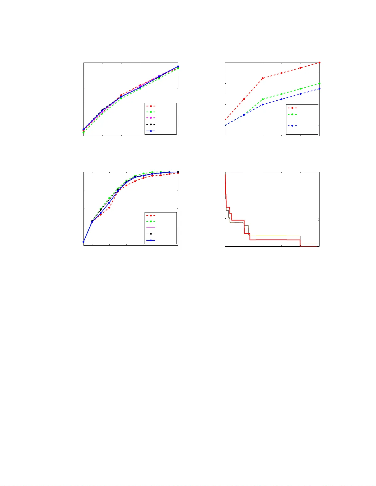
A D.C. Programming A pproac h to the Sparse Generalized Eigen v alue Problem Bharath K. Srip erum budur bhara thsv@ucsd.edu Dep artment of Ele ctric al and Comp ut er Engi ne ering University of Califo rnia, San Die go L a Jol la, CA 92093-0407, USA Da vid A. T orres da torres@cs.ucsd.edu Dep artment of Computer Scienc e and Engine ering University of Califo rnia, San Die go L a Jol la, CA 92093-0407, USA Gert R. G. Lanc kriet ger t@ece.ucsd. edu Dep artment of Ele ctric al and Computer Engine ering University of Califo rnia, San Die go L a Jol la, CA 92093-0407, USA Editor: Abstract In this paper , we consider the spa rse eig env alue pr oblem wherein the goal is to obtain a sparse solution to the genera lized eigenv alue problem. W e achiev e this by co nstraining the cardinality of the solution to the genera lized eigenv a lue problem and obtain spa rse prin- cipal comp onent analys is (PCA), sparse cano nical co rrelatio n ana ly sis (CCA) a nd sparse Fisher discriminant analysis (FD A) as sp ecia l cases. Unlik e the ℓ 1 -norm approximation to the ca r dinality constr a int, which previous metho ds have used in the context of s pa rse PCA, we prop ose a tighter approximation that is re lated to the neg ative log-likeliho o d of a Student’s t-distribution. The problem is then framed as a d.c. (difference of con- vex functions) progra m and is solv ed as a sequence of con vex progra ms by invoking the ma jorization-minimiza tio n metho d. The re sulting algo rithm is prov ed to ex hibit glob al c onver genc e behavior, i.e., for any rando m initialization, the s e quence (s ubs e quence) o f iterates g enerated by the alg o rithm conv erges to a stationary p o int of the d.c. progra m. The per formance of the algorithm is empirically demonstrated on b oth sparse PCA (finding few relev ant genes that explain as muc h v aria nc e as possible in a high- dimensional gene dataset) and spars e CCA (cros s-languag e do cument r etriev a l and vo c abulary selectio n for m usic retriev al) applicatio ns. Keyw ords: Generalized eigenv alue problem, Principal comp onent analysis, Ca nonical correla tion analysis, Fisher discriminant analysis , D.c. program, Ma jorization-minimiza tion, Global co nvergence analys is, Music a nnotation, Cr oss-lang uage do cument retriev al. 1. In t ro duction The generalized eigen v alue (GEV) prob lem for th e matrix pair ( A , B ) is the p roblem of finding a pair ( λ, x ) such that Ax = λ B x , (1) 1 where A , B ∈ C n × n , C n ∋ x 6 = 0 and λ ∈ C . When B is an identit y m atrix, the p roblem in (1) is simp ly referred to as an eigen v alue p roblem. Eigenv alue problems are so fund amen tal that they hav e applications in almost ev ery area of science and engineering (Strang, 1986) . In m ultiv ariate statistics, GEV pr oblems are pr ominen t and app ear in problems dealing with high-dimensional data analysis, visualization and pattern recognition. In these app li- cations, usually x ∈ R n , A ∈ S n (the set of symm etric matrices of size n × n defined o v er R ) and B ∈ S n ++ (set of p ositiv e defi nite matrices of size n × n defined o ve r R ). Th e v ariational form ulation for th e GEV pr oblem in (1) is giv en by λ max ( A , B ) = max { x T Ax : x T B x = 1 } , (GEV-P) where λ max ( A , B ) is the maxim um generalized eigen v alue asso ciated with the m atrix pair, ( A , B ). The x that maximizes (GEV-P) is called the generalized eigen ve ctor asso ciated with λ max ( A , B ). S ome o f the w ell-known and widely used data analysis techniques th at are s p ecific instances of (GEV-P) are: (a) Principal comp onent analysis (PCA) (Hotelli ng, 19 33; Jolliffe, 1986), a classic to ol for data analysis, data compression a nd v isu alizatio n, finds the direction of maximal v ariance in a giv en multiv ariate d ata set. This tec hnique is u sed in dimensionalit y reduction wher ein the a mbien t space in which the data resides is app ro ximated by a lo w-dimensional subspace without significan t loss of information. The v ariational form of PCA is obtained by c ho osing A to b e the co v ariance matrix (wh ic h is a p ositiv e semidefinite matrix defined o ver R ) associated with the m ultiv ariate data and B to b e the id entit y matrix in (GEV-P). (b) Canonical correlation analysis (CCA) (Hotelling, 1936), s im ilar to PC A, is also a data analysis and d imensionalit y reduction metho d. Ho wev er, while PCA deals w ith only one data space X (from which the m ultiv ariate data is obtained), C CA prop oses a wa y for dimensionalit y r eduction by t aking in to accoun t relations b et ween samples from t w o sp aces X and Y . The assumption is that the data p oints from these t w o spaces con tain some joint information th at is reflect ed in correlations b et w een them. Direc- tions al ong which this correlati on is high are th us assumed to b e rele v an t directions when these relations are to b e captured. The v ariational formulation for CCA is giv en b y max w x 6 = 0 , w y 6 = 0 w T x Σ xy w y p w T x Σ xx w x q w T y Σ y y w y , (2) where w x and w y are the directions in X and Y along whic h the data is maximally correlated. Σ xx and Σ y y represent the co v ariance matrices for X an d Y resp ectiv ely and Σ xy = Σ T y x represent s the cross-co v ariance matrix b et ween X a nd Y . (2) can b e rewritten as max { w T x Σ xy w y : w T x Σ xx w x = 1 , w T y Σ y y w y = 1 } , (3) whic h in turn can b e wr itten in the form of (GEV-P) with A =  0 Σ xy Σ y x 0  , B =  Σ xx 0 0 Σ y y  and x =  w x w y  . 2 (c) In th e binary classification s etting, Fisher discrimin an t analysis (FD A) fi nds a one- dimensional subspace, w ∈ R n , the pro jection of data on to wh ic h leads to maxima l separation b et ween th e classes. Let µ i and Σ i denote the mean vect or and co v ariance matrix associated with class i . The v ariational form ulation of FDA is giv en b y max w 6 = 0 ( w T ( µ 1 − µ 2 )) 2 w T ( Σ 1 + Σ 2 ) w , whic h can b e r ewritten as max w w T ( µ 1 − µ 2 )( µ 1 − µ 2 ) T w s.t. w T ( Σ 1 + Σ 2 ) w = 1 . (4) Therefore, the FD A form ulation is similar to (GEV-P) with A = ( µ 1 − µ 2 )( µ 1 − µ 2 ) T , called the b etwe en- cluster varianc e and B = Σ 1 + Σ 2 , called the within-cluster varianc e . F or multi- class problems, similar form ulations lead to multiple- discrim in an t analysis. Despite the simp licit y and p opularity of these data analysis and mo deling metho ds, one k ey drawbac k is the lac k of sparsity in their solution. They suffer from the disad v an tage that their solution v ector, i.e., x is a linear combination of all input v ariables, which often mak es it difficult to interpret the results. In the follo wing, we p oint to d ifferen t applications where P C A/CCA/FD A is u sed and motiv ate the need for spars e solutions. In man y PCA applications, the co ordin ate axes h a v e a p h ysical in terpretation; in b iology , for example, eac h axis migh t corresp ond to a sp ecific gene. In these cases, th e int erpr etation of the pr incipal comp onen ts wo uld b e f acilitated if they conta ined only few n on-zero en tries (or, loadings) while explainin g most of th e v ariance in th e data. Moreo v er, in certain app li- cations, e.g., fin ancial asset tr ad in g strategies based on PCA tec h niques, the sparsit y of the solution has imp ortant consequences, since fewer non-zero loadings imply fewer transaction costs. F or CC A, consider a d o cument translation ap p lication w here t w o copies of a corpu s of do cuments, one written in En glish and the other in German are giv en. Th e goal is to extract m ultiple lo w-dimensional r epresen tations of the do cuments, one in eac h language, eac h explaining most of the v ariation in the d o cument s of a single language while maximiz- ing the correlati on b et wee n the repr esen tations to aid translation. Sparse rep resen tations, equiv alen t to repr esen ting th e do cuments with a small set of words in eac h language, would allo w to int erpr et the underlyin g translation mec hanism and mo d el it b etter. In music annotation, CCA can b e applied to mo d el the correlation b et ween seman tic descriptions of songs (e.g., r eviews) and their acoustic con ten t. Sparsit y in the semanti c canonical comp o- nen ts would allo w to select the most meaningful w ords to d escrib e m usical con tent . This is exp ected to impro v e m usic annotation and r etriev al systems. In a classification setting lik e FD A, fea ture select ion aids generalization p erforman ce by promoting s p arse solutions. T o summarize, spars e r epresen tations are generally desirable as they aid h uman un derstanding, reduce compu tational and economic costs and pr omote b ette r generalizatio n. In this paper, w e consider the problem of finding sparse solutions while explaining the statistica l information in the d ata, w hic h can b e written as max { x T Ax : x T B x = 1 , k x k 0 ≤ k } , (SGEV-P) 3 where 1 ≤ k ≤ n and k x k 0 denotes the cardinalit y of x , i.e., the n umb er of non-zero elemen ts of x . The ab o v e program can b e sol ved either as a con tinuous optimization problem after relaxing the card inalit y constraint or as a discrete optimization pr oblem. In this pap er, we follo w the f ormer appr oac h . The fir st step in solving (SGEV-P) as a con tinuous optimization problem is to approximat e the cardinalit y constr aint. One usu al heuristic is to app ro ximate k x k 0 b y k x k 1 (see Section 2 f or the d etails on notation). Buildin g on the earlier v ersion of our w ork (Srip erumbudur et al., 2007), in this pap er, we ap p ro ximate the cardinalit y constrain t in (S GEV-P) as the negat ive log -lik eliho o d of a Student’s t-distribution, whic h has b een used earlier in many different con texts (W eston et al., 2003; F azel et al., 2003; Candes et al., 2 007). W e then form ulate this ap p ro ximate p r oblem as a d.c. (difference of con v ex fun ctions) program and s olv e it usin g the m a jorization-minimization (MM) metho d (Hun ter and Lange, 2004) resulting in a sequence of quadratically constrained quadratic programs (QCQPs). As a sp ecial case, when A is p ositive definite and B is an ident it y matrix (as is the case for PCA), a very simp le iterativ e u p date rule (w e call it as DC-PCA) can b e obtained in a closed f orm , which has a p er iteration complexit y of O ( n 2 ). S ince the prop osed algorithm is an iterativ e p ro cedure, using results fr om the global conv ergence theory of iterativ e algorithms (Z angwill, 1969), w e sho w that it is glob al ly c onver gent , i.e., for an y random initializatio n, the sequ ence (subsequence) of iterates generated by th e algorithm con v erges to a stationary p oint of th e d.c. p rogram (see Section 3.4 for a detailed definition). W e would lik e to m en tion th at the algorithm pr esen ted in this paper is more general than the one in Srip erumbudur et al. (2007) as it holds for any A ∈ S n unlik e in S rip eru mbudur et al. (2007), where A is assumed to b e p ositiv e semidefinite. W e illustrate the p erformance of the pr op osed algorithm on sparse PC A and sp arse CCA pr oblems. On the sparse PCA fron t, w e compare our results to SPC A (Zou et al., 2006) , DSPCA (d’Aspremon t et al., 2007 ), GSPCA (Moghaddam et al., 2007) and GP o wer ℓ 0 (Journ´ ee et al., 2008) in terms of sparsit y vs. explained v ariance on the “pit p rops” b enc h- mark dataset and a random test dataset. Since DSPCA an d GSPCA are n ot scala ble for large-scal e problems, we compare the p erforman ce of DC-PCA to SPCA and GP o w er ℓ 0 on three high-dimensional gene datasets w h ere the goal is to find relev an t genes (as few as p ossible) while exp laining the maxim um p ossible v ariance. The results show that DC-PCA p erforms similar to most of th ese algorithms and b etter than SPCA, b ut at b etter computa- tional sp eeds. The p rop osed sparse CCA algorithm is used in t w o spars e CC A applications, one d ealing w ith cross-language do cument retriev al and the other with vocabulary selection in m usic annotat ion. The cross-language document retriev al app lication in volv es a collec- tion of do cumen ts with eac h do cu m en t in d ifferen t languages, sa y English and F r enc h. The goal is, giv en a query string in one language, retrieve th e m ost r elev an t do cumen t(s) in the target language. W e exp erimen tally sh o w that the prop osed sparse CCA algorithm p erforms similar to the non-sparse version, h ow ever using only 10% of non-zero loadings in the canonical comp onents. In the vocabulary selection application, we show th at sp arse CCA imp ro v es the p erformance of a statistical m us ical query system by selecting only those w ords (i.e., pruning th e vocabulary) that are correlated to the underlying audio features. The pap er is organized as follo w s. W e establish th e mathematical notation in S ection 2. In Section 3, we p resen t the sparse generalized eigen v alue p roblem and discuss a tractable con v ex semidefin ite p rogramming (SDP) a pp ro ximation. Since the SDP appr o ximation is computationally intensiv e for large n , in Section 3.1, we presen t our prop osed app ro ximation 4 to the sparse GEV prob lem r esulting in a d .c. program. This is th en solv ed as a sequence of QCQPs in S ection 3.3 usin g the ma jorization-minimization metho d that is br iefly discuss ed in Section 3.2. The con v ergence analysis of the sparse GEV algorithm is present ed in Section 3.4. Finally , in Sections 4 and 5, we deriv e sparse PCA and sparse CCA as sp ecial instances of th e pr op osed algo rithm and present exp erimen tal resu lts to demons tr ate the p erformance, while in Secti on 6, we discuss the applicabilit y of the prop osed algorithm to the sparse FD A problem. 2. Notation S n (resp ectiv ely S n + , S n ++ ) denotes the set of symmetric (resp ectiv ely p ositiv e semidefinite, p ositiv e defin ite) n × n matrices defined o v er R . F or X ∈ S n , X ≻ 0 (resp ectiv ely X  0) means that X is p ositiv e d efinite (resp ectiv ely semidefin ite). W e denote a v ector of ones and zeros b y 1 and 0 respectiv ely . Depend ing on the context , 0 will also b e treated a s a zero matrix. | X | is the mat rix whose elemen ts are the absolute v alues of the elemen ts of X . [ X ] ij denotes the ( i, j ) th elemen t of X . F or x = ( x 1 , x 2 , . . . , x n ) T ∈ R n , x  0 d enotes an elemen t-wise inequalit y . k x k 0 denotes the num b er of non-zero elemen ts of the v ector x , k x k p := ( P n i =1 | x i | p ) 1 /p , 1 ≤ p < ∞ and k x k ∞ := m ax 1 ≤ i ≤ n | x i | . I n denotes an n × n iden tit y matrix. D ( x ) repr esen ts a d iagonal matrix formed w ith x as its principal d iagonal. 3. Sparse Generalized Eigenv alue P roblem As mentio ned in Section 1, the sparse generalize d eig env alue p roblem in (SGEV-P) can b e solv ed either as a cont inuous optimization prob lem after relaxing the cardinalit y constr aint or as a discrete optimization pr ob lem. In this section, w e consider the former approac h. Let us consider the v ariational formulatio n for the sparse generalized eigen v alue pr oblem in (SGEV-P), wh ere A ∈ S n and B ∈ S n ++ . Sup p ose A is not negativ e defin ite. T hen (SGEV-P) is the maximizatio n of a non-conca v e ob jectiv e o ver t he non-con ve x constraint set Φ := { x : x T B x = 1 } ∩ { x : k x k 0 ≤ k } . Although Φ can b e relaxed to a con vex set e Φ := { x : x T B x ≤ 1 } ∩ { x : k x k 1 ≤ k } , it do es not simplify the problem as the maximization of a non -conca ve ob j ective ov er a con vex set is still computationally h ard and in tractable [p. 342](Roc k afellar, 1970). 1 So, the in tractabilit y of (SGEV-P) is due to tw o reasons: (a) maximization of the non-conca ve ob jectiv e fu nction and (b) the constraint set b eing non-conv ex. Since (SGEV-P) is in tractable, instead of solving it dir ectly , one can solv e appro ximations to (SGEV-P) that are tractable. Differen t tractable app ro ximations to (SGEV-P) are p ossible, of which we briefly d iscu ss the con ve x semidefinite p rogramming (SDP) appro ximation and then motiv ate our prop osed n on-con v ex appr o ximation. First, let u s consider th e follo wing app r o ximate p rogram that is obtained by relaxing the non-con v ex constrain t set Φ to the con v ex set e Φ, as describ ed b efore: max { x T Ax : x ∈ e Φ } . (5) 1. Note th at (GEV- P) also invol ves the maximization of a non-concav e ob jectiv e ov er a non-conv ex set. How ever, it is w ell-known that p olynomial-time algorithms exist to solv e (GEV-P), which is due to its sp e cial structure of a q uadratic ob jective with a homogeneous qu adratic constraint (Bo yd an d V anden- b erghe, 2004, p. 229). 5 As men tioned b efore, this p rogram is still in tractable d ue to the maximization of the non- conca ve ob jectiv e. Had the ob jectiv e f u nction b een linear, (5) would hav e b een a canonical con v ex pr ogram, whic h could then b e solve d efficient ly . One appr oac h to linearize the ob jectiv e function is by using the lifting tec h nique (Lemar´ ec hal and Ou stry, 1999, Section 4.4), whic h was considered b y d ’Aspremon t et al. (2005) when A  0 and B = I n . The lifted v ersion of (5) is giv en by (see App en dix A f or details): max X , x tr( X A ) s.t. tr( X B ) ≤ 1 , k x k 1 ≤ k X = x x T . (6) Note that in the ab ov e p rogram, the ob jectiv e function is linear in X , and the constrain ts are con v ex exc ept for the non-conv ex co nstraint, X = x x T ( X = xx T ⇔ X  0 , rank( X ) = 1, where rank( X ) = 1 is a non-con vex constraint and therefore X = xx T is a n on-con v ex constrain t). Relaxing X = xx T to X − xx T  0 results in the follo w ing program max X , x tr( X A ) s.t. tr( X B ) ≤ 1 , k x k 1 ≤ k X − xx T  0 , (7) whic h is a s emid efinite p rogram (SDP) (V andenber gh e and Bo yd, 1996). Th e ℓ 1 -norm constrain t in (7) can b e relaxed as k x k 2 1 ≤ k 2 ⇒ 1 T | X | 1 ≤ k 2 so that the problem reduces to solving only for X . Therefore, we ha v e obtained a tractable con v ex approximat ion to (SGEV-P). Although (7) is a c onvex app ro ximation to (S GEV-P), it is compu tationally v ery in - tensiv e as general purp ose int erior-p oin t metho d s for SDP scale as O ( n 6 log ǫ − 1 ), where ǫ is the required accuracy on the optimal v alue. F or large-sc ale p roblems, first-order meth- o ds (Nestero v, 2005; d’Aspremont et al., 2007) can b e u sed wh ic h scale as O ( ǫ − 1 n 4 √ log n ). Therefore, the SDP-based con vex relaxation to (SGEV-P) is p rohibitiv ely exp ensiv e in com- putation for large n . In the follo wing s ection, we prop ose a different approxima tion to (SGEV-P), wherein instead of th e ℓ 1 -appro ximation to the cardinalit y constrain t, we consider a non-conv ex appro ximation to it. W e present a d.c. (difference of conv ex fu nctions) form ulation for this app ro ximation to (SGEV-P), w hic h is then solv ed as a sequence of QCQPs using the ma jorizatio n-min imization algorithm. 3.1 Non-conv ex approximation t o k x k 0 and d.c. formulation The p rop osed app ro ximation to (SGEV-P) is motiv ated by th e follo wing observ ations. • Because of the non-conca v e maximizatio n, a con v ex r elaxatio n of the cardinalit y con- strain t d o es not simp lify (SGEV-P). S o, a b etter approximati on to th e card in alit y constrain t than the tigh test con v ex relaxation, i.e., k x k 1 , can b e explored to impr o v e sparsit y . • Appr o ximations that yield go o d scalabilit y sh ould b e explored (as opp osed to, e.g., the SDP appr o ximation w hic h scales b adly in n ). 6 T o this end, w e consider the r egularized (p enalized) ve rsion of (SGEV-P) giv en b y max { x T Ax − ˜ ρ k x k 0 : x T B x ≤ 1 } , (SGEV-R) where ˜ ρ > 0 is the regularization (p enalizati on) parameter. Note that the qu adratic equalit y constrain t, x T B x = 1 is relaxed to the inequalit y constrain t, x T B x ≤ 1. Sin ce k x k 0 = n X i =1 1 {| x i |6 =0 } = lim ε → 0 n X i =1 log(1 + | x i | /ε ) log(1 + 1 /ε ) , (8) (SGEV-R) is equiv alen t 2 to max x x T Ax − ˜ ρ lim ε → 0 n X i =1 log(1 + | x i | /ε ) log(1 + 1 /ε ) s.t. x T B x ≤ 1 . (9) The ab o v e program is approximat ed b y th e f ollo win g appr oximate sp arse G EV pr o gr am by neglecting the limit in (9) and c ho osing ε > 0, max x x T Ax − ˜ ρ n X i =1 log(1 + | x i | /ε ) log(1 + 1 /ε ) s.t. x T B x ≤ 1 , (10) whic h is equiv alen t to max ( x T Ax − ρ ε n X i =1 log( | x i | + ε ) : x T B x ≤ 1 ) , (SGEV-A) where ρ ε := ˜ ρ/ log(1 + ε − 1 ). Note that the appr o ximate pr ogram in (SGEV-A) is a contin- uous optimizati on problem unlik e the one in (SGEV-R) , which has a com b inatorial term. Before w e presen t a d.c. program formulatio n to (SGEV-A), we briefly discu s s th e approx- imation to k x k 0 that we considered in this pap er. Appro ximation to k x k 0 : The appro ximation (to k x k 0 ) that w e consid er ed in this pap er, i.e., k x k ε := n X i =1 log(1 + | x i | ε − 1 ) log(1 + ε − 1 ) , has b een used in many d ifferen t co ntext s: feature selection u sing sup p ort v ector m ac h ines (W eston et al., 2003), sparse signal r eco very (Candes et al., 2007), m atrix rank minimization (F azel et al., 2003), etc. This appro ximation is in teresting b ecause of its connection to sparse factorial priors that are studied in Ba y esian inference, and can b e in terpreted as defin ing a Stud en t’s t-distribution p rior o v er x , an improp er prior give n by Q n i =1 1 | x i | + ε . Tipping (2001 ) show ed that this c hoice of prior le ads to a sparse representat ion and demonstrated its v alidit y for sparse k ernel expansions in the Ba y esian framew ork. Other ap p ro ximations 2. Tw o programs are equiv alent if their optimizers are the same. 7 to k x k 0 are p ossible, e.g., Bradley and Mangasarian (1998) us ed P n i =1 (1 − e − α | x i | ) with α > 0 ( k x k 0 = lim α →∞ P n i =1 (1 − e − α | x i | )) as an appr o ximation to k x k 0 in the co ntext of feature selectio n using supp ort ve ctor mac hin es. W e n o w sho w that the ap p ro ximation (to k x k 0 ) considered in this pap er, i.e ., k x k ε , is tigh ter than the ℓ 1 -norm app ro ximation, for any ε > 0. T o this end, let u s d efi ne a ε := log(1 + aε − 1 ) log(1 + ε − 1 ) , where a ≥ 0, so that k x k ε = P n i =1 | x i | ε . It is easy to c heck that k x k 0 = lim ε → 0 k x k ε and k x k 1 = lim ε →∞ k x k ε . In addition, we hav e a > a ε 1 > a ε 2 > . . . > 1 f or a > 1 and 1 > . . . > a ε 2 > a ε 1 > a for 0 < a < 1, if ε 1 > ε 2 > . . . , i.e., for any a > 0 and any 0 < ε < ∞ , the v alue a ε is closer to 1 than a is to 1. Th is m eans a ε for an y 0 < ε < ∞ is a b etter appr o ximation to 1 { a 6 =0 } than a is to 1 { a 6 =0 } . Th erefore, k x k ε for any 0 < ε < ∞ is a b etter approximat ion to k x k 0 than k x k 1 is to k x k 0 . Let u s d efine Q ( x ) := x T Ax − ˜ ρ k x k 0 , Q ε ( x ) := x T Ax − ρ ε n X i =1 log(1 + | x i | ε − 1 ) and Ω := { x : x T B x ≤ 1 } . Note that Q ( x ) = lim ε → 0 Q ε ( x ) for any fixed x , i.e., Q ε con v erges p oin t wise to Q . So, the sparse GEV problem is obtained as m ax { lim ε → 0 Q ε ( x ) : x ∈ Ω } , while the appr o ximate prob lem is give n b y max { Q ε ( x ) : x ∈ Ω } . Supp ose that b x denotes a maximizer of Q ( x ) o v er Ω and x ε denotes a maximizer of Q ε ( x ) o v er Ω. No w, one w ould lik e to kno w ho w go o d is the app ro ximate solution, x ε compared to b x . In general, it is n ot straigh tforward to either b ou n d k x ε − b x k in terms of ε or s h o w that k x ε − b x k → 0 as ε → 0 b ecause Q ( x ) may b e qu ite flat near i ts maxim u m o ve r Ω. A t least, one w ould lik e to kn o w w h ether Q ε ( x ε ) → Q ( b x ) as ε → 0, i.e., lim ε → 0 max x ∈ Ω Q ε ( x ) ? = max x ∈ Ω Q ( x ) = max x ∈ Ω lim ε → 0 Q ε ( x ) . (11) In other words, we w ould lik e to kno w w hether the limit pr o cess and the maximization o v er Ω can b e interc hanged. It can b e sho wn that if Q ε con v erges uniformly o v er Ω to Q , then the equalit y in (11) holds. Ho we ver, it is easy to see that Q ε do es not conv erge uniformly to Q o v er Ω , so nothing can b e said ab out (11). D.c. formulation: Let us return to the formulatio n in (SGEV-A). T o solv e this con tinuous, non-con v ex optimization pr oblem and derive an algorithm for the s parse GEV pr ob lem, we explore its formulati on as a d .c. program. D.c. p rograms are w ell studied and many algorithms exist to solv e them (Horst an d Thoai, 1999 ). Th ey are defined as f ollo ws. Definition 1 (D.c. program) L et Ω b e a c onvex set in R n . A r e al value d function f : Ω → R is c al le d a d.c. f u nction on Ω , if ther e exist two conv ex functions g , h : Ω → R such that f c an b e expr esse d in the f orm f ( x ) = g ( x ) − h ( x ) , x ∈ Ω . Optimization pr oblems of the form min { f 0 ( x ) : x ∈ Ω , f i ( x ) ≤ 0 , i = 1 , . . . , m } , wher e f i = g i − h i , i = 0 , . . . , m , ar e d.c. fu nctions ar e c al le d d.c. programs . 8 T o formulat e (SGEV-A) as a d.c. pr ogram, let u s c ho ose τ ∈ R such that A + τ I n  0. If A  0, such τ exists trivially (c h o ose τ ≥ 0). If A is ind efinite, choosing τ ≥ − λ min ( A ) ensures that A + τ I n  0. Therefore, c ho osing τ ≥ max(0 , − λ min ( A )) ensures that A + τ I n  0 for an y A ∈ S n . (SGEV-A) is equiv alen tly written as min x  τ k x k 2 2 − x T ( A + τ I n ) x  + ρ ε n X i =1 log( | x i | + ε ) s.t. x T B x ≤ 1 . (12) In tro d ucing the auxiliary v ariable, y , yields the equiv alent p rogram min x , y τ k x k 2 2 − " x T ( A + τ I n ) x − ρ ε n X i =1 log( y i + ε ) # s.t. x T B x ≤ 1 , − y  x  y , (13) whic h is a d.c. p rogram. In deed, the term τ k x k 2 2 is con v ex in x as τ ≥ 0 and , b y con- struction, x T ( A + τ I n ) x − ρ ε P n i =1 log( y i + ε ) is jointly con v ex in x and y . S o, the ab o ve program is a minimization of the difference of tw o con v ex fu nctions o ve r a conv ex set. Global optimization metho ds lik e branch and b ound, and cutting planes can b e u sed to solv e d .c. p rograms (Horst and T hoai, 1999), but are not scalable to large-scal e prob- lems. S ince (13) is a constrained nonlinear optimization p roblem, it can b e solv ed by , e.g., sequen tial qu adratic pr ogramming, augmente d Lagrangia n methods or redu ced-gradien t metho ds (Bonnans et al., 2006). In the follo wing sections, w e pr esen t an iterativ e algorithm to solve (13) using the ma jorization-minimization metho d . 3.2 Ma jorization-minimization metho d The m a jorization-minimization (MM) metho d can b e th ou ght of as a generalizat ion of the w ell-kno wn exp ectation-maximizat ion (EM) algorithm (Dempster et al., 1977). The general principle b eh in d MM algorithms w as fi r st en unciated by the numerical analysts O rtega and Rhein b oldt (1970) in the con text of line searc h metho d s. The MM principle app ears in man y places in statistical compu tation, includin g m ultidimens ional scaling (deLeeuw, 1977) , robust regression (Hub er, 1981), corresp ondence analysis (Heiser, 1987), v ariable selection (Hun ter and Li, 2005 ), sparse signal reco v ery (Can d es et al., 2007), etc. W e refer the intereste d reader to a tutorial on MM algorithms (Hunter and Lange, 2004) an d th e references therein. The general idea of MM algorithms is as follo ws. Su pp ose w e wan t to m in imize f ov er Ω ⊂ R n . The idea is to construct a majorization function g o ver Ω × Ω su c h that f ( x ) ≤ g ( x, y ) , ∀ x, y ∈ Ω and f ( x ) = g ( x, x ) , ∀ x ∈ Ω . (14) Th us , g as a function of x is an upp er b ound on f a nd coincides with f at y . T he ma jorizatio n-min imization algorithm corresp ond ing to this ma jorization f unction g u p dates x at iteration l by x ( l +1) ∈ arg min x ∈ Ω g ( x, x ( l ) ) , (15) 9 unless w e already ha ve x ( l ) ∈ arg m in x ∈ Ω g ( x, x ( l ) ) , in which case the alg orithm stops. The ma jorization function, g is usually constructed by using Jensen ’s inequalit y for con ve x functions, the fi rst-order T a ylor appro ximation or the quadratic u pp er b ound principle (B¨ ohning and Lin dsa y, 1988). Ho wev er, any other metho d can b e used to construct g as long as it satisfies (14). It is easy to show that the ab ov e iterativ e sc heme decreases the v alue of f m onotonically in eac h iteratio n, i .e., f ( x ( l +1) ) ≤ g ( x ( l +1) , x ( l ) ) ≤ g ( x ( l ) , x ( l ) ) = f ( x ( l ) ) , (16) where the first inequalit y and the last equalit y follo w from (14) while the sandwiched in- equalit y follo ws from (15). Note that MM algorithms can b e applied equally well to the maximization of f by simply reversing the inequ alit y sign in (14) and c hanging the “min” to “max” in (15). In this case, the word MM refers to minorization-maximization, wh er e the f unction g is called the minoriza tion function. T o put things in p ersp ectiv e, the EM algo rithm can b e obtained b y constructing the minorization function g using Jensen’s inequalit y for conca v e functions. T he construction of suc h g is r eferred to as the E-step, while (15) w ith the “min” replaced by “max” is referred to as th e M-step. The algorithm in (14) and (15) is us ed in mac hine learning, e.g., for non-negativ e m atrix f actoriza tion (Lee and Seu ng, 2001), und er the n ame auxiliary function metho d . Lange et al. (2000) studied th is algorithm u n der the name optimization tr ansfer while Meng (2000) r eferred to it as th e SM algorithm, where “S” stands for the surr ogate step (same as the ma jorization/minoriza tion step) and “M” stands for the minimization/maximiza tion step dep ending on the problem at hand . g is called the surrogate function. In the follo wing, w e consider an example that is relev ant to our problem where we construct a ma jorization function, g , whic h will late r b e u sed in deriving the sp ars e GEV algorithm. Example 1 (Linear Ma jorization) L et us c onsider the optimization pr oblem, min x ∈ Ω f ( x ) wher e f = u − v , with u and v b oth c onvex, and v c ontinuously differ entiable. Sinc e v is c onvex, we have v ( x ) ≥ v ( y ) + ( x − y ) T ∇ v ( y ) , ∀ x , y ∈ Ω . Ther efor e, f ( x ) ≤ u ( x ) − v ( y ) − ( x − y ) T ∇ v ( y ) =: g ( x , y ) . (17 ) It is e asy to verify that g is a ma jorization function of f . Ther efor e, we have x ( l +1) ∈ arg m in x ∈ Ω g ( x , x ( l ) ) = arg min x ∈ Ω u ( x ) − x T ∇ v ( x ( l ) ) . (18) If Ω is a c onvex set, then the ab ove pr o c e dur e solves a se quenc e of c onvex pr o gr ams. Note that the same ide a is use d in the c onc ave- c onvex pr o c e dur e (CCCP) (Y u il le and R angar ajan, 2003). Supp ose u and v ar e strictly c onvex, then a strict desc ent c an b e achieve d in (16) unless x ( l +1) = x ( l ) , i.e., if x ( l +1) 6 = x ( l ) , then f ( x ( l +1) ) < g ( x ( l +1) , x ( l ) ) < g ( x ( l ) , x ( l ) ) = f ( x ( l ) ) . (19) The first str ict ine quality fol lows fr om (17), a strict i ne quality for strictly c onvex v . Sinc e u is strictly c onvex, g is strictly c onvex and ther efor e g ( x ( l +1) , x ( l ) ) < g ( x ( l ) , x ( l ) ) unless x ( l +1) = x ( l ) . This strictly monotonic desc ent pr op erty wil l b e helpful to analyze the c on- ver genc e of th e sp arse GEV algorithm that is pr esente d in the fol lowing se ction. 10 3.3 Sparse GEV algorithm Let u s r etur n to the appro ximate sparse GEV program in (12). L et f ( x ) = τ k x k 2 2 + ρ ε n X i =1 log( ε + | x i | ) − x T ( A + τ I n ) x , (20) where τ ≥ max(0 , − λ min ( A )) so th at (12) can b e written as min x ∈ Ω f ( x ) and Ω = { x : x T B x ≤ 1 } . The main id ea in deriving th e sparse GEV alg orithm is in ob taining a ma jorizatio n fu nction, g that satisfies (14) and then usin g it in (1 5). The follo wing result pro vides suc h a f unction g for f in (20). Prop osition 2 The fol lowing f unction g ( x , y ) = τ k x k 2 2 − 2 x T ( A + τ I n ) y + y T ( A + τ I n ) y + ρ ε n X i =1 log( ε + | y i | ) + ρ ε n X i =1 | x i | − | y i | | y i | + ε , (21) majorizes f i n (20). Pro of C onsider th e term log ( ε + | x i | ) in f . Using the in equalit y log( z ) ≤ z − 1 , ∀ z ∈ R + with z = | x i | + ε | y i | + ε , w e ha v e log( ε + | x i | ) ≤ log ( ε + | y i | ) + | x i | − | y i | | y i | + ε , ∀ x , y . (22) On the other hand, since A + τ I n  0, by Example 1 with u ( x ) = τ k x k 2 2 and v ( x ) = x T ( A + τ I n ) x , we hav e τ k x k 2 2 − x T ( A + τ I n ) x ≤ τ k x k 2 2 − y T ( A + τ I n ) y − 2( x − y ) T ( A + τ I n ) y , ∀ x , y . (23) F rom (22) and (23), it is easy to c heck that g in (21) ma jorizes f o v er R n × R n and therefore o v er Ω × Ω where Ω = { x : x T B x ≤ 1 } . By follo w ing the min im ization s tep in (15) with g as in (21), the sp arse GEV algorithm is obtained as x ( l +1) = arg min x ( τ k x k 2 2 − 2 x T ( A + τ I n ) x ( l ) + ρ ε n X i =1 | x i | | x ( l ) i | + ε : x T B x ≤ 1 ) , (ALG) whic h is a sequence of quadratically constrained quadratic pr ograms (QCQP s ) (Bo y d and V anden b erghe, 2004). It is clear that x ( l +1) is the uniqu e optimal s olution of (ALG) ir- resp ectiv e of whether τ is zero or not. 3 (ALG) can also b e obtained b y app lyin g linear ma jorizatio n (see Example 1) to (13). See App en dix B for d etails. 3. Supp ose τ 6 = 0. The ob jectiv e fun ct ion in (ALG) is strictly conv ex in x and therefore x ( l +1) is the unique optimal solution. When τ = 0, th e ob jectiv e function is linear in x and th e unique optimum lies on the b oundary of the constraint set. 11 Assuming τ 6 = 0 and defin ing w ( l ) i := 1 | x ( l ) i | + ε , w ( l ) := ( w ( l ) 1 , . . . , w ( l ) n ) and W ( l ) := D ( w ( l ) ), a diagonal matrix w ith w ( l ) as its principal diagonal, (ALG) r educes to x ( l +1) = arg min x    x − ( τ − 1 A + I n ) x ( l )    2 2 + ρ ε τ    W ( l ) x    1 s.t. x T B x ≤ 1 . (24) (24) is v ery similar to LASS O (Tibsh irani, 1996) except for the weighte d ℓ 1 -p enalt y and th e quadratic constrain t. When x (0) is c h osen suc h that x (0) = a 1 , then the first iteration of (24) is a LASS O m inimization problem except for the quadratic constrain t. Let us analyze (24) to get an intuitiv e interpretation. (a) ρ ε = ˜ ρ = 0: (24) reduces to min {k x − s ( l ) k 2 2 : x T B x ≤ 1 } , wh er e s ( l ) = ( τ − 1 A + I n ) x ( l ) . S o, if s ( l ) ∈ { x : x T B x ≤ 1 } , th en x ( l +1) = s ( l ) , else x ( l +1) = ( I n + µ ( l +1) B ) − 1 s ( l ) , where µ ( l +1) satisfies [ s ( l ) ] T ( I n + µ ( l +1) B ) − 1 B ( I n + µ ( l +1) B ) − 1 s ( l ) = 1. The first term in the ob jectiv e of (24) compu tes the b est appr o ximation to s ( l ) in the ℓ 2 -norm so that the appro ximation lies in the ellipsoid x T B x ≤ 1. W e show in Corollary 6 that the iterativ e algorithm in (24) w ith ρ ε = 0 con v erges to the solution of (GEV-P) and therefore, the solution x is non-sp arse. (b) ρ ε = ˜ ρ = ∞ : In th is case, (24) reduces to min { k W ( l ) x k 1 : x T B x ≤ 1 } , w hic h is a w eigh ted ℓ 1 -norm minimization problem. Int uitivel y , it is clear th at if x ( l ) i is small, its w eigh ting f actor, w ( l ) i = ( | x ( l ) i | + ε ) − 1 in the next min imization step is large, wh ic h therefore pu s hes x ( l +1) i to b e small. This wa y the small entries in x are generally pushed to w ard zero as far as the co nstraints on x allo w, therefore yielding a sparse solution. F rom the ab ov e discussion, it is clear that (24) is a trade-off b et wee n the solution to the GEV problem and the solution to th e w eigh ted ℓ 1 -norm problem. F rom no w on, w e refer to (ALG) as the Sp arse GEV algorithm , which is detailed in Algorithm 1. T o run Algorithm 1, ˜ ρ , τ an d ε need to b e c hosen. In a sup ervised learning setup like FD A, ˜ ρ can b e chosen by cross-v alidation w hereas, in an unsup ervised setup lik e P C A/CCA, Algorithm 1 has to b e solv ed for v arious ˜ ρ an d the solution with desired cardin ality is selected. Since ˜ ρ is a free p arameter, τ and ε can b e set to any v alue (that satisfies the constrain ts in Algorithm 1) and ˜ ρ can b e tuned to obtain the desir ed sparsity as men tioned ab o ve . Ho wev er, it has to b e noted that for a fixed v alue of ˜ ρ , increasing τ or ε redu ces sparsit y . 4 So, in practice τ is c hosen to b e m ax(0 , − λ min ( A )), ε to b e close to zero and ˜ ρ is set by searc hing for a v alue th at p ro vides th e desired sparsity . Supp ose that Algorithm 1 outputs a solution, x ∗ suc h that k x ∗ k 0 = k . C an we say that x ∗ is the optimal solution of (SGEV-P) among all x with cardinalit y k ? Th e follo wing prop osition p ro vides a condition to c hec k for the non-optimalit y of x ∗ . In addition, it 4. Increasing ε increases t he approximation error b etw een k x k 0 and P n i =1 log(1+ | x i | ε − 1 ) log(1+ ε − 1 ) and th erefore re- duces sparsity . F rom (24), it is clear that increasing τ reduces th e weig ht on the term k W ( l ) x k 1 , which means more imp ortance is giv en to reducing the app roximation error, k x − ( τ − 1 A + I n ) x ( l ) k 2 2 , leading to a less sparse solution. 12 Algorithm 1 Sp arse Generalized Eigen v alue Algorithm Require: A ∈ S n , B ≻ 0, ε > 0 and ˜ ρ > 0 1: C ho ose τ ≥ max(0 , − λ min ( A )) 2: C ho ose x (0) ∈ { x : x T B x ≤ 1 } 3: S et ρ ε = ˜ ρ log(1+ ε − 1 ) 4: if τ = 0 then 5: rep eat 6: w ( l ) i = ( | x ( l ) i | + ε ) − 1 7: W ( l ) = D ( w ( l ) ) 8: x ( l +1) = arg max x x T Ax ( l ) − ρ ε 2    W ( l ) x    1 s.t. x T B x ≤ 1 . (25) 9: un til con ve rgence 10: else 11: rep eat 12: w ( l ) i = ( | x ( l ) i | + ε ) − 1 13: W ( l ) = D ( w ( l ) ) 14: x ( l +1) = arg min x    x − ( τ − 1 A + I n ) x ( l )    2 2 + ρ ε τ    W ( l ) x    1 s.t. x T B x ≤ 1 . (26) 15: un til con v ergence 16: end if 17: return x ( l ) also pr esen ts a p ost-pro cessing s tep (calle d var iational r enormalizatio n ) that impr oves the p erformance of Algorithm 1. See Moghaddam et al. (2007, Prop osition 2) for a similar result in the case of A  0 and B = I n . Prop osition 3 Supp ose Algorithm 1 c onver ges to a solution x ∗ such tha t k x ∗ k 0 = k . L et z b e the sub - ve ctor of x ∗ (obtaine d by r emoving the zer o entries of x ∗ ) and u k = arg max { x T A k x : x T B k x = 1 } , wher e A k and B k ar e su b matric es of A and B define d by the same non-zer o indic e s of x ∗ . If z 6 = u k , then x ∗ is not the optimal solution of (SGEV- P) among al l x with the same sp arsity p attern as x ∗ (and ther efor e, is not the optimal solution of (SGEV-P) among al l x with k x k 0 = k ). Nevertheless, by r eplacing the non-zer o entries of x ∗ with those of u k , the value of the obje ctive function in (SGEV-P ) incr e ases fr om [ x ∗ ] T Ax ∗ to λ ( A k , B k ) , its optimal v alue among al l x with the sa me sp arsity p attern as x ∗ . Pro of Assume that x ∗ , the solution output by Algorithm 1, is the optimal solution of (SGEV-P). D efine v su c h that v i = 1 {| x ∗ i |6 =0 } . Since x ∗ is the optimal so lution of (SGEV- P), w e ha ve x ∗ = arg max { y T D ( v ) AD ( v ) y : y T D ( v ) B D ( v ) y = 1 } , whic h is equiv alen t 13 to z = arg max { w T A k w : w T B k w = 1 } = u k and th e result follo ws. Note that λ ( A k , B k ) is th e optimal v alue of (SGEV-P) among all x with the same sparsit y pattern as x ∗ . Th er e- fore, if z = u k , then [ x ∗ ] T Ax ∗ = λ ( A k , B k ). The v ariational renormalization suggests that giv en a solution (in our case, x ∗ at the termi- nation of Algorithm 1 ), it is almost certainly b etter to discard the loadings, k eep only the sparsit y pattern and solv e the smaller un constrained su bproblem to obtain the final load- ings, given the sp arsit y pattern. Th is pro cedur e surely improv es an y con tin uous algorithm’s p erformance. In Algorithm 1, we mention that the iterativ e sc heme is con tin ued unti l con v ergence. What do es conv ergence mean here? Do es the algorithm really conv erge? If it con ve rges, what do es it conv erge to? Do es it con verge to an optimal solution of (SGEV-A)? T o address these questions, in the follo wing section, w e p ro vide th e conv ergence analysis of Algorithm 1 using to ols from global con v ergence theory (Zangwill, 1969). 3.4 C on v ergence analysis F or an iterativ e pr o cedure lik e Algorithm 1 to b e useful, it must conv erge to p oin t solu- tions from all or at least a s ignifi can t num b er of initialization states a nd n ot exhibit other nonlinear sys tem b eha viors, suc h as div ergence or oscillation. Glob al c onver genc e the ory of iter ative a lgorithms (Zangwill, 1969) can b e u sed to in v estigate th is b ehavio r. W e men tion up fr ont that this do es not deal with pr o ving conv ergence to a global optim um. Using this theory , recentl y , Srip erum bud ur and Lanckriet (2009) analyzed the conv ergence b eha vior of the iterativ e algorithm in (18) and sho we d that u nder certain conditions on u and v , the algorithm in (18) is globally con ve rgent, i.e., for any random initialization, x (0) , the sequence of iterates { x ( l ) } ∞ l =0 con v erges to some stationary p oin t 5 of th e d .c. program, min x ∈ Ω ( u ( x ) − v ( x )). Sin ce (ALG) can b e obtained b y applyin g linear ma jorization to (13), as sho wn in Ap p endix B, the con v ergence analysis of (ALG) ca n b e carr ied out ( see Theorem 5) b y inv oking the results in Srip eru m bud ur and Lanc kriet (2009 ). W e sh o w in Theorem 5 that Algorithm 1 is globally con v ergen t. In Corollary 6, we then show that Algorithm 1 con verge s to the solution of the GEV pr oblem in (GEV-P) when ˜ ρ = 0. In the follo w in g, we in tro duce s ome notation and terminology and then pro ceed with the deriv ation of the ab ov e mentio ned r esults. The conv ergence analysis of an iterativ e pro cedure like Algorithm 1 uses the n otion of a set- v alue d mapping , or p oint-to-set mapping , whic h is cen tral to the theory of global con v ergence. A p oin t-to-set map Ψ from a set X in to a set Y is defined as Ψ : X → P ( Y ), whic h assigns a subset of Y with eac h p oint of X , where P ( Y ) denotes th e p o wer set of Y . Ψ is said to b e uniformly c omp act on X if there exists a compact set H ind ep enden t of x suc h that Ψ( x ) ⊂ H for all x ∈ X . Note that if X is compact, then Ψ is un iformly compact on X . A fixe d p oint of the map Ψ : X → P ( X ) is a p oin t x for whic h { x } = Ψ( x ). Man y iterativ e algorithms in mathematical pr ogramming can b e d escrib ed using the notion of p oin t-to-set maps. Let X b e a set and x 0 ∈ X a give n p oin t. T hen an algorithm , A , with initial point x 0 is a p oin t-to-set map A : X → P ( X ) whic h generates a sequence 5. x ∗ is said to b e a stationary p oin t of a constrained optimization p roblem if it satisfies the corresp ond- ing Karush-Kuh n-T uck er (KKT) conditions (Bonnans et al., 2006, Section 13.3). Assuming constraint qualification, KK T cond itions are necessary for t he lo cal optimality of x ∗ . 14 { x k } ∞ k =1 via the rule x k +1 ∈ A ( x k ) , k = 0 , 1 , . . . . A is said to b e glob al ly c onver gent if for any chosen initial p oint x 0 , th e sequ ence { x k } ∞ k =0 generated b y x k +1 ∈ A ( x k ) (or a subsequen ce) con v erges to a p oint for whic h a necessary condition of optimalit y holds: the Karu sh-Kuhn - T uc ker (KKT) conditions in the case of constrained optimization and stationarit y in the case of unconstrained optimization. The prop ert y of global con v ergence expresses, in a sense, the certaint y that the algorithm w orks. It is v ery imp ortan t to s tress th e fact that it do es not imply (con trary to what the term m ight su ggest) conv ergence to a global optimum for all initial p oints x 0 . W e n o w sta te the con verge nce result for (18) by Srip erum bud ur and Lanckriet (2009), using w hic h w e pro vide the con vergence result for (ALG). Theorem 4 (Srip erum budur and Lanc kriet (2009)) Consid er the pr o gr am, min { u ( x ) − v ( x ) : x ∈ Ω } , (DC) wher e Ω = { x : c i ( x ) ≤ 0 , i ∈ [ m ] , d j ( x ) = 0 , j ∈ [ p ] } and [ m ] := { 1 , . . . , m } . L e t u and v b e strictly c onvex, differ entiable functions define d on R n . Also assume ∇ v is c ontinuous. L et { c i } b e differ entiable c onvex functions and { d j } b e affine f u nctions on R n . Supp ose (DC) is solve d iter atively as x ( l +1) ∈ A dc ( x ( l ) ) , wher e A dc is the p oint-to-set ma p define d a s A dc ( y ) = arg min x ∈ Ω u ( x ) − x T v ( y ) . (DC-ALG) L et { x ( l ) } ∞ l =0 b e any se q uenc e gener ate d by A dc define d by (DC-ALG). Sup p ose A dc is uni- formly c omp act on Ω and A dc ( x ) is nonempty for any x ∈ Ω . Then, assuming suitable c onstr aint qualific ation, al l the limit p oints of { x ( l ) } ∞ l =0 ar e stationary p oints of the d.c. pr o- gr am in (DC), u ( x ( l ) ) − v ( x ( l ) ) → u ( x ∗ ) − v ( x ∗ ) = : f ∗ as l → ∞ , for some stationary p oint x ∗ , k x ( l +1) − x ( l ) k → 0 , and either { x ( l ) } ∞ l =0 c onver ges o r the set of limit p oints of { x ( l ) } ∞ l =0 is a c onne cte d and c omp act sub set of S ( f ∗ ) , wher e S ( a ) := { x ∈ S : u ( x ) − v ( x ) = a } and S is the set of stationary p oints of (DC). If S ( f ∗ ) is finite, then any se quenc e { x ( l ) } ∞ l =0 gener ate d by A dc c onver ges to some x ∗ in S ( f ∗ ) . The fol lo wing global co nv ergence theorem for (ALG) is obta ined b y simply inv oking The- orem 4 with Ω = { ( x , y ) : x T B x ≤ 1 , − y  x  y } , u ( x ) = τ k x k 2 2 and v ( x , y ) = x T ( A + τ I n ) x − ρ ε P n i =1 log( y i + ε ). Theorem 5 (Global con v ergence of sparse GEV algorithm) L et { x ( l ) } ∞ l =0 b e any se- quenc e g ener ate d by the sp arse GEV algorithm in Algorith m 1. Then, al l the limit p oints of { x ( l ) } ∞ l =0 ar e statio nary p oints o f the pr o gr am in (SG EV -A), ρ ε n X i =1 log( ε + | x ( l ) i | ) − [ x ( l ) ] T Ax ( l ) → ρ ε n X i =1 log( ε + | x ∗ i | ) − [ x ∗ ] T Ax ∗ := L ∗ , (2 7) for some stationary p oint x ∗ , k x ( l +1) − x ( l ) k → 0 , and e i ther { x ( l ) } ∞ l =0 c onver ges or the set of limit p oints of { x ( l ) } ∞ l =0 is a c onne cte d and c omp act subset of S ( L ∗ ) , wher e S ( a ) := { x ∈ S : x T Ax − ρ ε P n i =1 log( ε + | x i | ) = − a } and S i s the set of stationary p oints of (SGEV-A). If S ( L ∗ ) i s finite, then any se quenc e { x ( l ) } ∞ l =0 gener ate d by Algorithm 1 c onver ges to some x ∗ in S ( L ∗ ) . 15 Pro of As noted b efore, (ALG) can b e obtained b y applying linear ma jorization to (13 ), whic h is equiv alen t to (SGEV-A), with Ω = { ( x , y ) : x T B x ≤ 1 , − y  x  y } , u ( x ) = τ k x k 2 2 and v ( x , y ) = x T ( A + τ I n ) x − ρ ε P n i =1 log( y i + ε ). It is easy to c hec k that u and v satisfy the conditions of Th eorem 4. Sin ce Algorithm 1 and (ALG) are equiv alen t, let A corresp ond to th e point-t o-set map in (ALG). Clearly { x : x T B x ≤ 1 } is compact and therefore A is uniformly compact. By the W eierstrass theorem 6 (Minoux, 1986 ), it is clear that A ( x ) is nonempty for any x ∈ { x : x T B x ≤ 1 } . The result therefore follo ws from Theorem 4. Ha ving consid ered the con verge nce of Algorithm 1, we now consider the con verge nce of sp ecial cases of Algorithm 1. Note that ˜ ρ = 0 imp lies ρ ε = 0. Using th is in (SGEV-A) yields the GEV problem in (GEV-P). Sin ce Algorithm 1 is derived based on (SGEV-A), it w ould b e of in terest to kno w whether the sequence { x ( l ) } ∞ l =0 generated b y Algorithm 1 for ˜ ρ = 0 c onv erges to the solution of (GEV-P) . The follo w ing corollary answ ers this and sho ws that wh en ˜ ρ = 0, t he solution of the sparse GEV algo rithm (Algorithm 1) matc hes with that of the GEV pr ob lem in (GEV-P). Corollary 6 L et ˜ ρ = 0 and λ max ( A , B ) > 0 . 7 Then, any se qu e nc e { x ( l ) } ∞ l =0 gener ate d by Algor ithm 1 c onver ge s to some x ∗ such that λ max ( A , B ) = [ x ∗ ] T Ax ∗ and [ x ∗ ] T B x ∗ = 1 . Pro of The stationary p oin ts of (SGEV-A) with ρ ε = ˜ ρ = 0 are the generalized eigen v ectors of ( A , B ). T h erefore, the set S as defined in Theorem 5 is fi nite and any sequence { x ( l ) } ∞ l =0 generated b y Algorithm 1 con verges to some x ∗ in S ( L ∗ ) where L ∗ = − [ x ∗ ] T Ax ∗ . W e n eed to s h o w that L ∗ = − λ max ( A , B ). Note th at x ∗ is a fixed point of Alg orithm 1. Consider (ALG) wh ic h is equiv alen t to Algorithm 1. With ρ ε = 0, solving the Lagrangian yields x ( l +1) = ( µ ( l +1) B + τ I n ) − 1 ( A + τ I n ) x ( l ) , wher e µ ( l +1) ≥ 0 is the Lagrangian du al v ariable for the constrain t [ x ( l +1) ] T B x ( l +1) ≤ 1. A t the fi xed p oint, x ∗ , we h a v e ( µ ∗ B + τ I n ) x ∗ = ( A + τ I n ) x ∗ whic h implies Ax ∗ = µ ∗ B x ∗ . (28) Multiplying b oth s ides of (28) by [ x ∗ ] T , w e ha v e [ x ∗ ] T Ax ∗ = µ ∗ [ x ∗ ] T B x ∗ = µ ∗ ([ x ∗ ] T B x ∗ − 1) + µ ∗ = µ ∗ , (29) where we ha v e in vok ed the complementary slac kness condition, µ ∗ ([ x ∗ ] T B x ∗ − 1) = 0. T he optim um v alue of (ALG) at the fixed p oin t is giv en b y ψ ∗ := − 2[ x ∗ ] T Ax ∗ − τ k x ∗ k 2 2 , whic h b y (29) reduces to ψ ∗ = − 2 µ ∗ − τ k x ∗ k 2 2 . It is easy to see that making µ ∗ > 0, and therefore [ x ∗ ] T B x ∗ = 1 minimizes ψ ∗ instead of c ho osing µ ∗ = 0 and [ x ∗ ] T B x ∗ < 1. Since ψ ∗ is minimized by choosing th e maxim um µ ∗ that satisfies (28), ( µ ∗ , x ∗ ) is ind eed the eigen pair that satisfies the GEV p roblem in (GEV-P). In addition to ˜ ρ = 0, su pp ose A  0 and τ = 0. Then, the follo wing result sho ws that a simple iterativ e algorithm can b e obtained to compu te th e generalized eigen v ector associated with λ max ( A , B ). 6. The W eierstrass theorem states: If f is a real contin uous function on a compact set K ⊂ R n , then the problem min { f ( x ) : x ∈ K } has an optimal solution x ∗ ∈ K . 7. If λ max ( A , B ) > 0, then max { x T Ax : x T B x ≤ 1 } = max { x T Ax : x T B x = 1 } = λ max ( A , B ). 16 Algorithm 2 Sp arse PCA algorithm (DC-PCA) Require: A  0, ε > 0 and ˜ ρ > 0 1: C ho ose x (0) ∈ { x : x T x ≤ 1 } 2: S et ρ ε = ˜ ρ log(1+ ε − 1 ) 3: rep eat 4: w ( l ) i = ( | x ( l ) i | + ε ) − 1 5: x ( l +1) i = h   ( Ax ( l ) ) i   − ρ ε 2 w ( l ) i i + sign(( Ax ( l ) ) i ) r P n i =1 h   ( Ax ( l ) ) i   − ρ ε 2 w ( l ) i i 2 + , ∀ i (31) 6: until con ve rgence 7: ret urn x ( l ) Corollary 7 L et A  0 , τ = 0 and ˜ ρ = 0 . Then, any se q u enc e { x ( l ) } ∞ l =0 gener ate d by the fol lowing algorithm x ( l +1) = B − 1 Ax ( l ) p [ x ( l ) ] T AB − 1 Ax ( l ) (30) c onver ges to some x ∗ such that λ max ( A , B ) = [ x ∗ ] T Ax ∗ and [ x ∗ ] T B x ∗ = 1 . Pro of Consider (ALG) with τ = 0 and ρ ε = ˜ ρ = 0. Since the ob jectiv e is linear in x , the minim um occurs at th e b oundary of the co nstr aint set, i.e ., { x : x T B x = 1 } . S olving the Lagrangian, we get (30). The result therefore follo ws from Corollary 6 which holds for an y τ ≥ 0. So far, we hav e prop osed a sparse GEV algorithm and p r o v ed its global conv ergence b ehavi or. In th e follo wing sections (Sections 4-6), w e consider sp ecific in stances of the sparse GEV pr oblem and use the prop osed algorithm (Algorithm 1) to add ress th em. 4. Sparse Principal Comp onen t A nalysis In this s ection, w e consider sp arse PC A as a sp ecial case of the sparse GEV algorithm that w e presented in Section 3.3. Based on the sparse GEV algorithm in Algorithm 1, we prop ose a spars e PCA algorithm, called DC-PCA, w ith A  0 b eing th e co v ariance matrix, B = I n and τ = 0. In this sett ing, (ALG) reduces to a v ery simple iterativ e ru le, whic h is pro v ed in App endix C: x ( l +1) i = h   ( Ax ( l ) ) i   − ρ ε 2 w ( l ) i i + sign(( Ax ( l ) ) i ) r P n i =1 h   ( Ax ( l ) ) i   − ρ ε 2 w ( l ) i i 2 + , ∀ i, (ALG-S) where [ a ] + := max(0 , a ). Th e corresp ond in g spars e PCA algorithm (DC-PCA) is sh o wn in Algorithm 2. Note that the compu tation of x ( l +1) , from x ( l ) , in v olv es co mpu ting Ax ( l ) , whic h has a complexit y of O ( n 2 ). Therefore, the DC-PC A algorithm has a p er iteration complexit y of O ( n 2 ). Since Algorithm 1 exhibits the global conv ergence b eh a vior and DC- 17 PCA is a sp ecial case of Algorithm 1, it follo ws th at DC-PCA exhibits the global con ve rgence prop erty . Supp ose ρ ε = ˜ ρ = 0. Th en , with A  0 and B = I n , (SGEV-R) redu ces to: max { x T Ax : x T x = 1 } , (EV-P) i.e., a stand ard eigen v alue problem. Th erefore, it is of interest to kno w wh ether Algorithm 2 pro vides a solution of (EV-P) when ˜ ρ = 0. It f ollo ws fr om Corollary 7 that DC-PCA con v erges to a solution of (EV-P) when ˜ ρ = 0. In ad d ition, th e follo wing resu lt sho ws that DC-PCA redu ces to the p o wer metho d for computing λ max ( A ) w h en ˜ ρ = 0. Prop osition 8 (P o w er metho d) Supp ose ˜ ρ = 0 . Then, Algorithm 2 is the p ower metho d for c omputing λ max ( A ) . Pro of S etting ˜ ρ = 0 in Algorithm 2 yields x ( l +1) = Ax ( l ) k Ax ( l ) k 2 , (32) whic h is the p o wer iteration for the computation of λ max ( A ). Before pr o ceeding fur ther, we br iefly discuss th e prior w ork on sparse PCA algorithms. The earliest attempts at “sparsifyin g” PC A consisted of simple axis rotations and com- p onent th r esholding (Cadima and Jolliffe, 1995) for su bset selection, often b ased on the iden tification of p rincipal v ariables (McCab e, 1984). The fir st true computational tec h- nique, called S CoTLASS (Jolliffe et al., 2003) , pr o vided an optimization framework us- ing LASSO (Tibshirani, 1996) b y enf orcing a sparsit y constrain t on the PCA solution by b ound ing its ℓ 1 -norm, leading to a non-conv ex p ro cedure. Zou et al. (2006) prop osed a ℓ 1 -p enalized regression algorithm for PCA (called SPCA) using an elastic net (Zou and Hastie, 2005) and solv ed it v ery efficien tly using least angle regression (Efron et al., 2004). Subsequ ently , d’Asp remon t et al. (2007) p rop osed a con vex r elaxation to the n on-con v ex cardinalit y constraint for PCA (called DSPCA) leading to a SDP with a complexit y of O ( n 4 √ log n ). Although this method sho ws p erformance comparable to S PCA on a small- scale b enc hmark data set, it is n ot scalable for high-dimensional data sets, ev en p ossib ly with Nestero v’s first-order metho d (Nestero v, 20 05). Moghaddam et al. (2007) p rop osed a com binatorial optimization algorithm (called GS P CA) using greedy searc h and b ranc h-and- b ound metho ds to solv e the sparse PCA problem, leading to a to tal complexity of O ( n 4 ) for a f ull set of solutions (one for eac h target s p arsit y b et w een 1 and n ). d’Asp remon t et al. (2008) formulated a new SDP relaxatio n to the sparse PC A problem an d derived a more efficient greedy algorithm (compared to GSP CA) for computing a f ull set of solutions at a total numerical complexit y of O ( n 3 ), which is based on the con ve xit y of the largest eigen v alue of a symmetric matrix. Recen tly , Journ´ ee et al. (200 8) prop osed a simple, ite r- ativ e and very efficien t sparse PCA a lgorithm (GP o w er ℓ 0 ) with a p er iteration complexit y of O ( n 2 ), whic h is based on the idea of linear ma jorization. T h ey show ed that it p erforms similar to man y of the ab o ve men tioned algorithms. Therefore, to our kn o wledge, GPo we r ℓ 0 is the state-of-the-art. In the f ollo win g, we discuss ho w DC-PCA relat es to SCoTLASS (Jolliffe et al., 2003), SPCA (Z ou et al., 2006) and GP o wer ℓ 0 (Journ´ ee et al., 2008). W e then present exp eriments to empir ically compare different approac hes. 18 4.1 C omparison to SCoTLASS As men tioned b efore, the SC oTLASS program is obtained by approximati ng k x k 0 with k x k 1 in (SGEV-P) and is give n by max x x T Ax s.t. k x k 2 2 = 1 , k x k 1 ≤ k , (33) where A  0. Let us consider the regularized v ersion of the ab ov e program, giv en b y max x x T Ax − ρ k x k 1 s.t. k x k 2 2 ≤ 1 . (34) It is clear that (34) is not a canonical con v ex program b ecause of the con ve x maximization. Applying th e MM algorithm to (34), we obtain the follo wing iterativ e algorithm: x ( l +1) = arg max x x T Ax ( l ) − ρ 2 k x k 1 s.t. k x k 2 2 ≤ 1 . (35) Using an appr oac h as in App endix C, (35) can b e solved in closed form as x ( l +1) i =    ( Ax ( l ) ) i   − ρ 2  + sign(( Ax ( l ) ) i ) q P n i =1    ( Ax ( l ) ) i   − ρ 2  2 + , ∀ i. (36) No w, let us compare (36) with the DC-PC A iteration in Algorithm 2. F or ScoTLASS , x ( l +1) i = 0 if | ( Ax ( l ) ) i | ≤ ρ 2 , wh ereas for DC-PCA, x ( l +1) i = 0 if | ( Ax ( l ) ) i | ≤ ρ ε 2 w ( l ) i . This means that if x ( l ) i = 0 for some l , then DC-PCA ensu r es that x ( m ) i = 0 , ∀ m > l w h ic h is not guaran teed for SCoTLASS . Therefore, DC-PCA ensures faster con v ergence of an irrelev ant feature to zero than SCoTLASS, thus pro vid in g b etter sparsit y . This is not surprisin g as a better appro x im ation to the cardinalit y constrain t is u s ed in DC-PCA. It can b e shown that when ρ = 0, lik e DC-PCA, SCoTLASS also reduces to the p ower iter ation algorithm in (32). 4.2 C omparison to SPCA Let Q b e a r × n matrix, where r and n are the num b er of observ ations and the num b er of v ariables resp ectiv ely , w ith the column means b eing zero. Supp ose Q h as an SVD giv en by Q = U Λ V T , where U con tains the p rincipal comp onen ts of un it length and t he columns of V are the corresp onding loadings of the prin cipal comp onents. Let y i = [ U Λ ] i , ∀ i . Zou et al. ( 2006, Theorem 1) p osed PCA as a regression problem and s h o w ed t hat [ V ] i = x ⋆ / k x ⋆ k 2 , where x ⋆ = arg min x k y i − Q x k 2 2 + λ k x k 2 2 , (37) where λ > 0. This is equ iv alen t to solving for an eigenv ector of Q T Q =: A . Th erefore, solving for t he e igenv ectors of a p ositiv e semidefinite matrix is p osed as a ridge regression 19 problem in (37). T o solv e for sp ars e eigen vect ors, Zou et al. (2006 ) in tro d uced an ℓ 1 -p enalt y term in (37) resulting in the follo wing elastic net called SPCA, x ′ = arg min x k y i − Q x k 2 2 + λ k x k 2 2 + λ 1 k x k 1 , (38) where λ 1 > 0. This problem can b e inte rp reted in a Ba y esian setting as follo ws : give n the lik eliho o d on y i , y i | x , σ 2 ∼ G ( Qx , σ 2 I ), whic h is a circular normal random v ariable with mean Qx (conditioned on x ), and a prior distrib ution on x , x | β 2 , γ ∼ G ( 0 , β 2 I ) Q i exp( − γ | x i | ), whic h is the p ro duct of a circular Gaussian and a pro d u ct of Laplacian d ensities, compute the maximum a p osteriori (MAP) estimate of x . It is easy to see th at the p enalization parameters λ and λ 1 in (38) are related to σ 2 , β 2 and γ . As aforemen tioned, our app roac h can b e interpreted as definin g an im p rop er prior ov er x , w hic h pr omotes sparsit y (Tip- ping, 2001). W e use p ( x ) ∝ Q i 1 | x i | + ε (instead of Q i exp( − γ | x i | )) as the pr ior suc h that x | β 2 , ε ∼ G ( 0 , β 2 I ) p ( x ). Replacing th e p rior in (38) with our prior, results in min x || y i − Q x || 2 2 + λ || x || 2 2 + λ 1 X i log( | x i | + ε ) . (39) Since the p r oblem in (39) is equiv alent to (SGEV-A) with B = I n , it is clear that DC-PCA can b e exp ecte d to pr o vide sparser solutions than SPC A b ecause of the pr ior p ( x ) that promotes sparsit y . It is to b e noted that the SPCA f ramew ork is not extendible to other settings like FD A or CCA unlik e our formulatio n whic h is generic. 4.3 C omparison to GP o wer ℓ 0 Consider the follo wing regularized sparse PCA p rogram wher e A  0: max { x T Ax − ˜ ρ k x k 0 : x T x ≤ 1 } . (40) In our case, w e approxi mated k x k 0 b y k x k ε and p osed the a pp ro ximate pr ogram as a d .c. program, resulting in DC-PCA obtained thr ough m a jorization-minimization. On the other hand, without u sing an y approxi mations to k x k 0 , Journ´ ee et al. (2008) s h o w ed that the solution to (40) can b e obtained as: x i =  sign(( c T i z ) 2 − ˜ ρ )  + c T i z q P n i =1  sign(( c T i z ) 2 − ˜ ρ )  + ( c T i z ) 2 , ∀ i, (41 ) where A = C T C , C is a p × n matrix, c i is the i th column of C and z is the solution to the follo win g pr ogram wh ic h is the maximization of a con v ex fu nction o ve r an ellipsoid: max ( n X i =1  ( c T i z ) 2 − ˜ ρ  + : k z k 2 2 = 1 , z ∈ R p ) . (42) (42) is then solv ed iterativ ely (called GPo wer ℓ 0 ) using a simple gradient-t yp e scheme r esult- ing in the follo win g up date rule: z ( l +1) = n X i =1 h sign(( c T i z ( l ) ) 2 − ˜ ρ ) i + c T i z ( l ) c i , z ( l +1) = z ( l +1) k z ( l +1) k 2 . 20 T able 1: Loadings for fi rst three s parse principal comp on ents (PCs) of the p it props data. The SP C A and DSPCA loadings are tak en from Zou et al. (2006) and d’Aspr emon t et al. (2007) resp ectiv ely . PC x 1 x 2 x 3 x 4 x 5 x 6 x 7 x 8 x 9 x 10 x 11 x 12 x 13 1 -.48 -.48 0 0 .18 0 -.25 -.34 -.42 -.40 0 0 0 SPCA 2 0 0 .79 .62 0 0 0 -.02 0 0 0 . 01 0 3 0 0 0 0 .64 .59 .49 0 0 0 0 0 -.02 1 -.56 -.58 0 0 0 0 -.26 -.10 -.37 -.36 0 0 0 DSPCA 2 0 0 .71 .71 0 0 0 0 0 0 0 0 0 3 0 0 0 0 0 -.79 -.61 0 0 0 0 0 .01 1 .44 .45 0 0 0 0 .38 .34 .40 .42 0 0 0 GSPCA 2 0 0 .71 .71 0 0 0 0 0 0 0 0 0 3 0 0 0 0 0 .82 .58 0 0 0 0 0 0 1 .44 .45 0 0 0 0 .38 .34 .40 .42 0 0 0 GP ow er ℓ 0 2 0 0 .71 .71 0 0 0 0 0 0 0 0 0 3 0 0 0 0 0 .82 .58 0 0 0 0 0 0 1 .45 .46 0 0 0 0 .37 .33 .40 .42 0 0 0 DC-PCA 2 0 0 .71 .71 0 0 0 0 0 0 0 0 0 3 0 0 0 0 0 .82 .58 0 0 0 0 0 0 It can b e sho wn that their gradien t-t yp e s c heme is equiv alen t to an MM-t yp e algorithm. Therefore, our metho d differs from GP ow er ℓ 0 only in a small w a y . This is al so confir med empirically in t he follo w ing subsection where DC-PC A a nd GPo w er ℓ 0 exhibit similar per- formance. W e w ould like to ment ion that unlike our sparse generalized eigen v alue algorithm (Algorithm 1), GPo we r ℓ 0 cannot b e readily extended to settings like FD A and CCA. 4.4 Exp erimen tal results In this section, we illustrate the effectiv en ess of DC-PCA in terms of sparsity and scalabilit y on v arious datasets. On small datasets, the p erformance of DC-PCA is compared against SPCA, DSPC A, GSPCA and GP o wer ℓ 0 , wh ile on large datasets, DC-PCA is compared to all these algorithms except DSPCA and GS P CA due to scalabilit y issues. Sin ce GP o w er ℓ 0 has b een compared to the greedy algorithm of d’Aspremont et al. (2008) by J ourn´ ee et al. (2008 ), wherein it is sho wn that these t w o algorithms p erform similarly except for the greedy algorithm b eing compu tationally more complex, we do not include the greedy algorithm in our comparison. The results sho w that the p er f ormance of DC-PCA is comparable to the p erformance of many of these algo rithm s, but with b e tter sc alability . Th e exp eriment s in this pap er are carr ied out on a Lin ux 3 GHz, 4 GB RAM wo rkstation. On the implementa tion side, w e fix ε to b e the mac hine precision in all our exp er im ents, wh ic h is motiv ated from the discussion in Section 3.1. 4.4.1 Pit pr ops da t a The pit p rops dataset (Jeffers, 1967) has b ecome a standard b enchmark example to test sparse PCA algorithms. The first 6 principal comp onen ts (PC s) ca ptu r e 87 % of the total v ariance. Ther efore, the explanato ry p ow er of sparse PCA metho ds is often co mpared on 21 the first 6 sparse PCs. 8 T able 1 sh o ws the fi r st 3 sparse PCs and their loadings for SPCA, DSPCA, GSPCA, GP o w er ℓ 0 and DC-PCA. Usin g the fi r st 6 sparse PCs, S PCA captures 75.8% of the v ariance with a card in alit y pattern of (7 , 4 , 4 , 1 , 1 , 1), which ind icates the n umb er of n on-zero loadings for the first to the sixth sp arse PC, resp ectiv ely . Th is r esults in a total of 18 non-zero loadings for SP CA, w h ile DSPCA captures 75.5% of the v ariance with a sparsity pattern of (6 , 2 , 3 , 1 , 1 , 1), totaling 14 non-zero loadings. With a sparsity pattern of (6 , 2 , 2 , 1 , 1 , 1) (total of only 13 non-zero loadings), DC-PCA, GSPCA and GP o we r ℓ 0 can capture 77.1% of the total v ariance. Comparing the cu m ulativ e v ariance and cum ulative cardinalit y , Figures 1(a–b) show that DC-PC A explains more v ariance with fewe r non- zero loadings th an SPCA and DSP CA. In add ition, its p er f ormance is similar to that of GSPCA and GPo wer ℓ 0 . F or the firs t sparse PC , Figure 1(c) shows that DC-PCA consistent ly explains more v ariance with b ette r sparsit y than SPCA, wh ile p erforming similar to other algorithms. Figure 1(d) shows th e v ariation of sparsit y and explained v ariance with resp ect to ˜ ρ for th e fi rst spars e PC computed w ith DC-PC A. T his plot sum marizes the metho d f or setting ˜ ρ : the algorithm is ru n for v arious ˜ ρ and the v alue of ˜ ρ that ac hieve s the desired sparsit y is selecte d. 4.4.2 Random test p roblems In this section, we follo w the exp erimental setup that is consider ed in Jou r n ´ ee et al. (2008). Throughout this section, we assu me A = C T C , w here C is a p × n random matrix whose en tries are ge nerated according to a Gaussian distribution, with zero mean a nd unit v ari- ance. In the follo w in g, w e p resen t the trade-off cu r v es (prop ortion of explained v ariance vs. cardinalit y for the fir st sp arse PC asso ciated w ith A ), computational complexit y vs. cardi- nalit y and compu tational complexit y v s . problem size f or v arious spars e PCA algorithms. T rade-off curv es. Figure 2(a) sh o ws the trade-off b et wee n the prop ortion of explained v ariance and the card inalit y for the fir st sparse PC asso ciated with A for v arious sparse PCA algorithms. F or eac h algorithm, th e sp arsit y in ducing parameter ( k in the case of DSPCA and GSPC A, and the regularization parameter in the case of SP CA, GP o we r ℓ 0 and DC-PCA) is in cremen tally increased to obtain the solution v ector with cardinalit y that decreases from n to 1. The resu lts d ispla y ed in Figure 2(a) are av erages of computations on 100 random matrices with dimens ions p = 100 and n = 300. It can b e seen from Figure 2(a) that DC-PCA p erforms similar to DSPC A, GSPCA and GPo wer ℓ 0 , while p erform ing b etter than S PCA. Computational complexit y vs. C ardinalit y . Figure 2(b) shows the av erage time required b y the spars e PCA algorithms to extract the fir st sparse PC of A with p = 100 and n = 300, f or v arying card in alit y . It is ob vious from Figure 2(b) that as th e cardinalit y increases, GSPCA tends to get slow er while the sp eed of SPC A, GPo w er ℓ 0 and DC-PCA is not r eally affected by the cardinalit y . W e did not sho w the results of DSPCA in Figure 2(b) as its computational complexit y is an order of magnitude (around 100 times) more than 8. The discussion so far dealt with compu ting the first sparse eigenv ector of A . T o compu te the subsequ ent sparse eigen vectors, usually the sparse PCA algorithm is app lied to a sequence of deflated matrices. See Mac key (2009) for details. In th is pap er, we used the orthogonalized Hotelling’s deflation as mentioned in Mack ey (2009). 22 1 2 3 4 5 6 30 40 50 60 70 80 Number of principal components Cumulative Variance (%) SPCA DSPCA GSPCA GPower 0 DC−PCA (a) 1 2 3 4 5 6 4 6 8 10 12 14 16 18 Number of principal components Cumulative cardinality SPCA DSPCA GSPCA GPower 0 DC−PCA (b) 2 4 6 8 10 12 0.2 0.4 0.6 0.8 1 Cardinality Proportion of explained variance SPCA DSPCA GSPCA GPower 0 DC−PCA (c) 0 9 18 27 36 45 0.5 1 Proportion of explained variance 0 9 18 27 36 45 5 10 ρ ~ Cardinality (d) Figure 1: Pit props: (a) cum ulativ e v ariance and (b) cu mulativ e cardinalit y for the fi rst 6 sparse principal comp onen ts (PCs ); (c) p rop ortion of explained v ariance (PEV) vs. cardinalit y for the first sp arse P C (obtained b y v arying the sparsit y parameter and computing the cardin alit y and exp lained v ariance for the solution v ector); (d) dep end en ce of sparsit y and PEV on ˜ ρ for the fi rst sparse PC computed with DC- PCA. the scale on the ve rtical axis o f Figure 2(b). Journ´ ee et al. (2008) h a v e demonstr ated that the greedy metho d pr op osed by d’Aspr emon t et al. (2008) also exhibits the b eha vior of increasing compu tational complexity with the increase in cardinalit y . Computational complexit y vs. Problem size. Figure 3 sho ws the a verag e compu - tation time in seconds, required by v arious sparse PCA algorithms, to extract the first sparse PC of A , for v arious pr ob lem sizes, n , where n is in creased exp onen tially and p is fixed to 500. The times shown are a ve rages ov er 100 random instances of A for eac h p rob- lem s ize, where the sparsit y ind u cing parameters are c hosen su ch that the solution v ectors of these algorithms exhibit comparable cardinalit y . It is clear from Figure 3 that DC-PCA and GPo we r ℓ 0 scale b etter to large-dimensional problems than th e other algorithms. S ince, on a verag e, GSPCA and DSPCA are muc h slow er than the other metho ds, eve n for lo w car- 23 0 60 120 180 240 300 0.3 0.4 0.5 0.6 0.7 0.8 0.9 1 Cardinality Proportion of explained variance SPCA DSPCA GSPCA GPower 0 DC−PCA (a) 0 60 120 180 240 300 10 −2 10 −1 10 0 10 1 10 2 Cardinality Computational time (sec) GSPCA SPCA GPower 0 DC−PCA (b) Figure 2: Random test data: (a) (a ve rage) prop ortion of explained v ariance vs. cardinalit y for th e fir st sparse PC of A ; (b) (a verag e) computation ti me vs. cardinalit y . I n (a), al l the sp ars e PCA a lgorithms p erform simila rly and b etter than S PCA. In (b), the complexit y of GS P CA grows significan tly with incr easing cardinalit y of the solution vecto r, while the sp eed of the other metho ds is a lmost indep endent of the cardinalit y . 10 1 10 2 10 3 10 4 10 −4 10 −2 10 0 10 2 10 4 n Computational time (seconds) SPCA DSPCA GSPCA GPower 0 DC−PCA Figure 3: Av erage computation time (seconds) for the fi rst sparse PC of A vs. problem size, n , ov er 100 randomly generated matrices A . dinalities ( see Fig ur e 2(b)), we discard t hem from all the follo wing n umerical e xp erimen ts that d eal with large n . F or the remaining algorithms, SPC A, GP o wer ℓ 0 and DC-PCA, we run another round of exp eriments, no w examining the computational complexit y with v arying n and p but with a fixed asp ect ratio n/p = 10. The results are dep icted in T able 2. Again, the corresp onding regularization p arameters are set in s u c h a w a y that the solution ve ctors of these algorithms exhibit comparable cardinalit y . Th e v alues display ed in T able 2 corresp ond to the a v erage runn in g times of the algorithms on 100 ran d om instances of A f or eac h pr oblem size. It can b e seen t hat our prop osed metho d , DC-PCA, is comparable to GP o we r ℓ 0 and faste r than SPCA. 24 T able 2: Av erage computation time (in seconds) for the first s p arse PC asso ciated with A for a fixed regularization parameter. p × n 100 × 1000 250 × 2500 500 × 5000 750 × 7500 1000 × 10000 SPCA 0.135 1.895 10.256 34 .367 87.459 GP o we r ℓ 0 0.027 0.159 0.310 1.224 1.904 DC-PCA 0.034 0.151 0.301 1.202 1.913 T able 3: Gene exp ression d atasets Dataset S amples ( p ) Genes ( n ) Re ference Colon cancer 62 2000 Alon et al. (1999 ) Leuk emia 3 8 7129 Golub et al. (1999) Ramasw am y 127 16063 Ramasw am y et al. (2001 ) 4.4.3 Gene expression d a t a Gene exp r ession data from DNA microarrays p ro vides the expression lev el of thousand s of genes across several h und reds or thousands of exp eriments. T o enhance the in terp retation of these large data sets, sparse PCA algorithms can b e applied, to extract sp arse pr incipal comp onent s that inv olv e only a f ew genes. Datasets. Usually , gene expression data is sp ecified by a p × n matrix (sa y C ) of p samples and n genes. T h e co v ariance matrix, A is therefore computed as C T C . In our exp eriments, we consider three gene expr ession datasets w hic h are tabulated in T able 3. The c olon cancer datase t (Alon et al., 1999) consists of 62 tissu e samples (22 n orm al an d 40 cancerous) with the gene exp r ession profiles of n = 2000 genes extracted from DNA microarra y data. Its firs t principal comp onent explains 44.96% of the tota l v ariance. Th e leuk emia dataset (Golub et al., 1999) consists of a trainin g s et of 38 samples (27 ALL and 11 AML, tw o v arian ts of leuk emia) from b one marr o w sp ecimens and a test set of 34 sam- ples (20 ALL and 14 AML). This dataset has b een used w id ely in classification settings where the goal is to distinguish b et ween t wo v ariants o f leuk emia. All samples ha ve 7129 features, eac h of whic h corresp onds to a normalized gene expression v alue extracted from the microarray image. The first principal comp onent exp lains 87.64% of the total v ariance. The Ramasw am y dataset has 16063 genes and 127 s amp les, its fir st principal comp onent explaining 76.5% of the total v ariance. The h igh dimen sionalit y of these d atasets make s them suitable candidates for studying the p erformance of s p arse PCA algorithms, by in v estigating their abilit y to explain v ariance in the data based on a small num b er of genes, to obtain in terpretable results. Since DSPCA and GSPCA are not scalable for these large datase ts, in our stu d y , w e compare DC-PCA to S P CA and GP o w er ℓ 0 . T rade-off curves . Figures 4(a-c) sh o w the pr op ortion of explained v ariance versus the 25 T able 4: Computation time (in sec onds) to obtain the first sparse PC, a verag ed o v er car- dinalities ranging from 1 to n , for the Colo n cancer, Leukemia and Ramaswam y datasets. Colon cancer Leukemia Ramaswam y n 2000 7 129 16063 SPCA 2.0 57 3.548 38.731 GP o we r ℓ 0 0.182 0.223 2 .337 DC-PCA 0.034 0.156 0 .547 cardinalit y for the first sparse PC for th e datasets sho wn in T able 3. It can b e seen that DC-PCA p erforms similar to GPo wer ℓ 0 and p erforms b etter than SPCA. Computational complexit y . The a v erage computation time requ ired b y the sp arse P C A algorithms on eac h dataset is sho wn in T able 4. T h e indicated times are a verage s o ve r n computations, one for eac h cardin alit y ranging fr om n do wn to 1. The results sh ow that DC-PCA and GP o w er ℓ 0 are s ignifican tly faster than SPCA, whic h, for a long time, was widely accepted as the algorithm that can h andle large datasets. Ov erall, the results in this s ection demonstrate that DC-PCA p erforms similar to GP o wer ℓ 0 , the state-of-the-a rt, and b etter than SPCA, b oth in terms of scalabilit y and prop ortion of v ariance explained vs. cardinalit y . W e w ould lik e to men tion that our sparse PCA algo- rithm (DC-PCA) is deriv ed from a more general framew ork, that can b e used to address other generalize d eig env alue p roblems as w ell, e.g., sparse C CA, sp arse FD A, etc. 5. Sparse Canonical Correlation Analysis In this section, w e consider spars e C CA as a sp ecial case of the sparse GEV algorithm and present tw o CCA applications w here sp arsit y is helpful. W e call our sp arse CC A algorithm DC-CCA, w here A an d B are determined from the co v ariance and cross-co v ariance matrices as explained right b elo w (3). Not e that A is indefi nite and, therefore, in our experim ents, w e c ho ose τ = − λ min ( A ) in Algorithm 1. In the follo wing, w e p resen t tw o sparse CCA applications, one related to the task of cross-language do cument retriev al and the other dealing w ith semant ic annotation and retriev al of music (T orres et al., 2007a,b). The sp ars e CC A algorithm considered in this section wa s earlier pr op osed by us in T orres et al. (2007b). Related work inv olv es the sparse CCA algorithm due to Hardo on and Sha we-T a ylor (2008). In S ection 3, w e pr esen ted a S DP relaxation, whic h could b e applied for s p arse CC A. Ho wev er, in th is section, w e use DC-CCA (based on Algorithm 1) to p erform sparse CCA, as it scales b etter for large pr ob lem sizes. W e illustrate its p erformance in the ab o ve mentio ned applications. 26 0 500 1000 1500 2000 0 0.2 0.4 0.6 0.8 1 Cardinality Proportion of explained variance GPower 0 DC−PCA SPCA (a) 0 2000 4000 6000 0 0.2 0.4 0.6 0.8 1 Cardinality Proportion of explained variance GPower 0 DC−PCA SPCA (b) 0 5000 10000 15000 0 0.2 0.4 0.6 0.8 1 Cardinality Proportion of explained variance GPower 0 DC−PCA SPCA (c) Figure 4: T rade-off cu rv es b et ween explained v ariance and cardinalit y for (a) Colon can- cer, (b ) Leuke mia and (c) Ramasw amy datasets. The prop ortion of v ariance explained is computed on the first sp arse pr incipal comp onent. (a– c) sho w that DC-PCA p erforms similar to GP o wer ℓ 0 , while exp laining m ore v ariance (for a fixed cardinalit y) than SPCA. 5.1 C ross-language document retriev al The problem of cross-language do cument r etriev al in vol ves a collection of do cument s, { D i } N i =1 with eac h do cument b eing r epresen ted in d ifferen t languages, sa y English and F renc h. The goal of the task is, giv en a query string in one language, retriev e the most relev an t do cu- men t(s) in the target language. The fi rst step is to obtain a semant ic representa tion of the do cuments in b oth languages, whic h mo dels the correlation b et ween tran s lated versions, so w e can d etect similarities in con tent b etw een th e t w o d o cumen t sp aces (one for English and the other for F ren c h). This is exactly what CCA do es b y fi nding a low-dimensional rep- resen tation in b oth languages, with maximal correla tion b et we en them. Vinok our o v et al. (2003 ) used CCA to address this pr ob lem and sho we d that the CCA appr oac h p erforms b etter th an the laten t seman tic indexing app roac h u sed by Littman et al. (1998 ). C CA 27 pro vides an efficient basis repr esen tation (that captures the maximal correlation) for the t w o do cumen t sp aces. Using a bag-of-w ords represen tation f or the do cuments, sp arse C CA w ould allo w to find a lo w-dimens ional m o del based on a s m all sub s et of words in both languages. This w ould impro ve the int erpr etabilit y of the mo del and could id en tify small subsets of words that are u sed in similar context s in b oth languages and, p ossib ly , are translations of one an- other. Repr esen ting do cuments b y their similarity to all other do cuments (e.g., b y taking inner pr o ducts of bag-of-w ord ve ctors, as exp lained b elo w), sp ars e CCA would create a lo w-dimensional mo del that only requir es to measure the similarit y for a small sub s et of the training do cumen ts. T his would immediately impro ve storage requirements and th e effi- ciency of retriev al computations. In this study , we follo w the second appr oac h , rep resen ting do cuments by their simila rity to all ot her trainin g do cuments by a pp lying a linear k ernel function to a binary bag -of-w ords represen tation of the do cum en ts, as prop osed in Vinok- ouro v et al. (2003). T h is will illustrate h o w w e can achiev e significan t sparsit y without significan t loss of r etriev al p erformance. More s p ecifically , eac h version of a do cum en t (English or F renc h) is mo deled u sing a bag-of-w ord s feature vec tor. Within a feature vecto r, w e asso ciate an element in { 0 , 1 } with eac h word w i in its language vocabulary . A v alue of 1 ind icates that w i is found in the docum ent. W e collect the feature v ectors in to the N × P matrix E , where w e co llect the English feature v ectors, and the N × Q matrix F , wh er e w e collect the F ren ch feature v ectors. N is the num b er of do cuments and P and Q are the v o cabulary sizes of E an d F resp ectiv ely . Computing the sim ilarity b etw een English do cum ents as the inn er p ro duct b et wee n their binary bag-of-w ords vec tors (i.e., the rows of E ) r esults in compu tin g an N × N data matrix E E T . Similarly , we compute an N × N d ata matrix F F T and obtain t w o feature spaces w hic h are b oth N -dimensional. By applying sp arse CCA, we effec tive ly p erform simultaneous feature selection across t w o vec tor sp aces and characte rize the con ten t of and correlation b et ween English and F renc h d o cument s in an efficien t mann er. W e use the DC-C C A algorithm, us ing th e co v ari- ance and cross-v ariance matrices asso ciated w ith the do cu m en t matrices E E T and F F T and obtain successiv e pairs of sp arse canonical comp onen ts which w e stac k into the columns of V E and V F . (Su bsequent pairs of these sparse canonical comp onen ts are obtained by deflating E E T and F F T with resp ect to previous canonical comp onents. F or a detailed review on deflation, w e refer the reader to Sha we- T aylor and Chr istianini (2004).) Then, giv en a q u ery do cument in an input language, sa y English, w e conv ert th e query in to the appropriate feature v ector, q E . W e pro ject q E on to the subsp ace sp anned by the sparse canonical comp onen ts in the English language space by computing V T E q E 9 . Similarly , w e pr o ject all the F rench do cuments ont o the subs p ace sp anned b y th e sparse canonical com- p onents, V F asso ciated w ith the F renc h language . Finally , w e perf orm do cument retriev al b y selec ting those F rench do cu m en ts wh ose pro jections a re close st to th e pro jected query , where we measure distance in a nearest neigh b or sense. 9. Notice how this pro jection, onto the sparse canonical components, on ly requires to compute a few elemen ts of q E , i.e., the ones correspond ing to the non-zero loadings of the sparse canonical components; differently said, we only need to compu te the similarit y of the q uery do cument to a small sub set of all training d ocuments. 28 T able 5: Av erage area un der the ROC curve (in %) using C C A and spars e CCA (DC- CCA) in a cross-language d o cumen t retriev al task. d r epresen ts the num b er of canonical comp onents and sp arsity repr esen ts the p ercentag e of zero loadings in the canonical comp onen ts. d 100 200 300 400 500 CCA 99.92 99.93 99.96 99.95 99.93 DC-CCA 95.72 97.57 98.45 98.75 99.04 Sparsit y 87.1 5 87.56 87.95 88.21 88.44 5.1.1 Experiment al Det ails The data s et used w as th e Aligned Hansards of the 36th P arliament of Canad a (Ger- mann, 2001), w h ic h is a collection of 1 .3 milli on pairs of text c hunks (sen tences or sm aller fragmen ts) aligned into English and F renc h translations. The text ch u nks are split in to do cuments based on ∗ ∗ ∗ delimiters. After removing stop w ords and rare w ords (those that o ccur less than 3 times), we are left with an 1800 × 26328 English do cument-b y-term matrix and a 1800 × 30167 F renc h matrix. Computing E E T and F F T results in matrices of size 1800 × 1800. T o generate a query , we select English test do cuments from a test set not u sed for training. The appr opriate retriev al result is the corresp onding F rench language v ersion of the query do cument. T o p erform r etriev al, the quer y and the F rench test d o cument s are pr o jected on to the sparse canonical comp onents and retriev al is p erformed as describ ed b efore. T able 5 sh o ws the p erform ance of DC-CC A (sp arse CCA) against C CA. W e measure our results using the a verag e area und er the R OC cur v e (a ve rage AR OC). The results in T able 5 are sho wn in p ercen tages. T o go into detail, for eac h test query we generate an R OC curv e from the rank ed r etriev al resu lts. Results are ranked according to their pro jected feature v ector’s Euclidean distance from the query . The area under this R OC curve is used to measure p erformance. F or example, if the first r eturned do cument was the most relev ant (i.e., the corresp on d ing F rench language v ersion of the q u ery document) this would resu lt in an R OC with area under t he curv e (AR OC) of 1. If t he most relev ant d o cument came in ab o ve the 75 th p ercent ile of all d o cumen ts, this wo uld lead to an AROC of 0.75, and so on. So, we’re basically measuring ho w highly th e corresp onding F renc h language do cum en t ranks in th e r etriev al results. F or a collection of queries we take the simple a verag e of eac h query’s AROC to obtain the av erage AR OC. An av erage AR OC of 1 is b est, a v alue of 0.5 is as go o d as chance. In T able 5, w e compare retriev al using sparse CCA to r egular CCA. F or sparse CCA, w e use a sp ars it y p arameter that le ads to loadings that are app ro ximately 1 0% of the f u ll dimensionalit y , i.e., the canonical comp onen ts are appro ximately 90% sparse. W e note that sparse CC A is able to ac h iev e go o d retriev al rates, only sligh tly sacrificing p erforman ce com- pared to regular CCA. This is t he key result of t his section: we can ac hiev e p erformance close to regular CC A, b y using only ab out 12% of th e n umb er of loadings (i.e., do cum en ts) required by regular CCA. This s h o ws that sp arse CC A can n arro w in on the most informa- 29 tiv e dimensions exhibited by data and can b e used as an effecti ve dim en sionalit y reduction tec h nique. 5.2 V o cabulary selection for m usic information retriev al In this subsection we pro vide a sh ort summary of the resu lts in T orr es et al. (2007a), which nicely illustrate ho w sparse CCA can b e used to impro v e the p erformance of a statistical m usical qu ery application, by id en tifying prob lematic qu ery wo rd s and eliminating th em from the mo del. The application in vo lve s a computer audition system (T urnbull et al., 2008) that can annotate songs with semantic ally meaningful words or ta gs (such a s, e.g., r o ck or mel low ), or retriev e songs fr om a database, b ased on a semantic query . Th is system is based on a joint prob ab ilistic mo d el b et w een words an d a coustic s ignals, learned from a training data set of songs and song tags. “Noisy” words, th at are n ot or only w eakly r elated to the musical con ten t, will d ecrease the system’s p erformance and w aste compu tational resources. S parse CCA is employ ed to pru ne aw a y th ose noisy w ords and impro ve th e system’s p erformance. The details o f this exp erimen t are beyond the scop e of th is w ork and can be found i n T orres et al. (2007a) . In short, eac h song from the C AL-500 dataset 10 is r epresen ted in t w o differen t spaces: in a semantic space, based on a bag-of-w ords repr esen tation of a song’s seman tic tags, and in an audio space, based on Mel-frequency cepstral co efficien ts (Mc kin- ney , 2003) extracted fr om a song’s audio conten t. T his representat ion allo ws sparse C C A to iden tify a small su bset of w ords spanning a semant ic su bspace that is highly correlated with audio con ten t. In Figure 5, we u se sparse CCA t o generate a sequence of v o cabularies of progressiv ely sm aller size, ranging from f u ll size (con taining ab out 180 w ords) to very sp ars e (con taining ab out 20 words), depicted on the h orizonta l axis. F or eac h v o cabulary size, the computer audition system is trained and the a v erage area un der the receiv er op erating char- acteristic curv e (AR OC) is sho wn on the v ertical axis, measurin g its retriev al p erformance on an ind ep endent test set. Th e AR OC (ranging b et ween 0.5 for r andomly ranked retriev al results and 1.0 for a perf ect r an k in g) initially clearly impr o v es, a s sparse CCA (DC-CCA) generates vocabularies of smaller size: it is effectiv ely remo vin g n oisy w ords that are detri- men tal for the sys tem’s p erformance. Also sho wn in Figure 5 are the r esults of training the m usic r etriev al s y s tem based on tw o alternativ e v o cabulary selection techniques: rand om selection (offering no improv ement) and a heuristic that eliminates wo rd s exhibiting less agreemen t amongst the human su b jects that w ere s u rv eye d to collect the CAL-500 dataset (only offering a sligh t improv ement , in itially). In summary , T orres et al. (2007a ) illustrates that v o cabulary selection u sing sparse CCA significantl y improv es the retriev al p erformance of a computer audition system (by effectiv ely r emo ving noisy words), outp erforming a random b aseline and a human agreemen t heuristic. 10. The CAL-500 data set consists of a set of songs, annotated with semantic tags, obtained by conducting human surveys. More details can b e found in T urnbull et al. (2008). 30 180 140 100 60 20 0.68 0.7 0.72 0.74 0.76 Average AROC Vocabulary size DC−CCA Human agreement Random Figure 5: Comparison of vocabulary selection tec hn iques for music r etriev al. 6. Sparse Fisher Discriminan t A nalysis In this sec tion, w e sho w that the FD A problem is an inter esting sp ecial case of the GEV problem and that the sp ecial structure of A allo ws the sparse FD A problem to b e so lved more efficien tly than the general sparse GEV pr oblem. Let us consider the GEV problem in (GEV-P) with A ∈ S n + , B ∈ S n ++ and rank( A ) = 1. This is exactly the FD A problem as sh own in (4) where A is of the form A = aa T , with a = ( µ 1 − µ 2 ) ∈ R n . The corresp onding GEV problem is w ritten as λ max ( A , B ) = max x ( a T x ) 2 s.t. x T B x = 1 , (43) whic h can also be written as λ max ( A , B ) = max x 6 = 0 ( a T x ) 2 x T Bx . S ince w e are p rimarily in ter- ested in the maximizer of (43), w e can rewrite it as min x 6 = 0 x T B x ( a T x ) 2 ≡ min { x T B x : a T x = 1 } . (44) The adv an tage of the form ulation in (44) w ill b ecome clear w h en we consider its sp arse v ersion, i.e., after in tro ducing the c onstraint { x : k x k 0 ≤ k } in (44). Clearly , in tro du cing the sp arsit y constrain t makes the problem in tractable. Ho we ve r, int ro d ucing an ℓ 1 -norm relaxation in this form ulation giv es rise to a c onvex pr o g r am , min { x T B x : a T x = 1 , k x k 1 ≤ k } , (45) more sp ecificall y a q u adratic p rogram (QP), and the corresp ondin g p enalized v ersion is giv en b y min { x T B x + ν k x k 1 : a T x = 1 } , (46) where ν > 0 is the regularization parameter. 31 Note th at a tran s formation s imilar to th e one leading to (44) can b e p erformed f or the GEV problem w ith an y , general A ∈ S n , i.e., writing the GEV problem as a minimizatio n problem, min x x T B x s.t. x T Ax = 1 . (47) This f orm ulation, ho wev er, is not usefu l to simplify solving a GEV pr oblem in general. Indeed, consider the s p arse ve rsion of the pr oblem in (47) with the s p arsit y constrain t { x : k x k 0 ≤ k } relaxed to { x : k x k 1 ≤ k } . Because of the quadr atic equality constraint , the resulting program is non-con v ex for an y A . Supp ose th at the constrain t set { x : x T Ax = 1 } is relaxed to { x : x T Ax ≤ 1 } . If A ∈ S n \ S n + , the program is still n on-con v ex as the constrain t d efines a non-con v ex set. If A ∈ S n + , then the optim um o ccurs at x = 0 . Therefore, the minimizati on form ulation of the GEV problem in (47) is not useful, unlik e the case where A ∈ S n + and r ank( A ) = 1. Based on the discu ssion so far, it i s clear that the sparse FDA problem c an b e solved as a con vex QP , whic h is significan tly more efficien t than, e.g., an SDP relaxation as in (7) for sparse PCA or sp arse CC A. Supp ose that one wo uld like to use a b etter appr oximati on to k x k 0 than k x k 1 , for sparse FD A. Using the app ro ximation w e considered in this work, (45) r educes to min x x T B x + ν ε n X i =1 log( ε + | x i | ) s.t. a T x = 1 , (48) where ν ε := ν / log (1 + ε − 1 ). Ap plying the MM metho d to the ab ov e program results in the follo w in g iterativ e sc h eme, x ( l +1) = arg min x x T B x + ν ε n X i =1 | x i | | x ( l ) i | + ε s.t. a T x = 1 , (49) whic h is a sequence of QPs un lik e Alg orithm 1, wh ic h is a sequence of QCQPs. Th e nice structure of A mak es the corresp ondin g sparse GEV problem computationally efficient. Therefore, one should solve the sp arse FD A problem by using (45) or (49) instead of u sing the con v ex SDP in (7) or Algorithm 1. Suyke ns et al. (2002, S ection 3.3) and Mik a et al. (2001, Prop osition 1) ha ve sho wn connections b et we en the FD A form ulation in (44) with a = µ 1 − µ 2 and B = Σ 1 + Σ 2 (see paragraph b elo w (4) f or details) and least-squares sup p ort vecto r mac hines (classifiers th at minimize the squ ared loss, see Suykens et al. (2002 , C h apter 3)). T h erefore, sparse FD A is equiv alen t to feature selection with least-squares su pp ort ve ctor mac hines. In other w ords, (45) is equiv alent to LASSO, while the form ulation in (48) is similar to the one considered in W eston et al. (2003). Since these are well studied problems, we do not pursue further sho wing the numerical p erformance of sparse FDA . 32 7. Conclusion and Discussion W e s tudy the p roblem of fi n ding sparse eigen vec tors for generalized eigen v alue problems. After p rop osing a non-con vex but tigh t approximat ion to the cardinalit y constrain t, we form ulate the resulting optimization problem as a d.c. p rogram and derive an iterativ e algorithm, based on the ma jorization-minimizati on metho d . T his results in s olving a se- quence of q u adratically constrained quadratic programs, an algorithm which exhibits global con v ergence b eha vior, as w e show. W e also derive spars e PCA (DC-PCA) and sparse CCA (DC-CCA) algorithms as sp ecial cases of our pr op osed algorithm. Empirical results d emon- strate th e p erformance of the p rop osed algorithm for sp ars e PCA and sparse CCA applica- tions. In the c ase of sparse PCA, we exp erimen tally d emonstrate on b oth b enc hmark and real-life d atasets of v arying dimensionalit y that the prop osed algorithm (DC-PCA) explains more v ariance with sparser f eatures than SP C A (Zou et al., 2006) while p erforming simi- larly to DSPCA (d’Aspremont et al., 2007) and GSPCA (Moghaddam et al., 2007) at b etter computational sp eed (lo w er CPU time). O n the other h and, DC-PCA has p erforman ce and scalabilit y similar to that of the state-of-the-a rt GP o w er ℓ 0 algorithm. W e also illustrate the practical relev ance of th e s parse CC A algorithm in t w o ap p lications: cross-language do cument r etriev al and v o cabulary s election f or music information retriev al. The p rop osed algorithm do es n ot allo w to set the regularization parameter a priori, to guarant ee a giv en sparsity lev el. This is similar for SPCA and GP o wer ℓ 0 . S DP-based relaxation metho d s , on the other h and (e.g., DSPCA in the con text of sparse PCA) are b etter suited to achiev e a give n sparsit y lev el in one shot, by incorp orating an explicit constrain t on the sparsity of the solution (although, ev ent ually , through r elaxatio n, an appro ximation of the original problem is solv ed). S ince the a lgorithm w e p rop ose solve s a LASSO problem in eac h step b ut w ith a qu adratic constraint, one could explore using a mo dified v ersion of path follo wing tec hniques like least angle regression (Ef r on et al., 2004) to learn the en tire regularization path. Ac kno wledgmen ts Bharath Srip erumbudur thanks Suvrit Sr a for constructiv e discussions wh ile the former was an in tern at the Max Planc k Institute for Biological Cyb ernetics, T ¨ ubingen. The a uth ors wish to ac kn o wledge su pp ort fr om the National Science F ound ation (grant DMS-MSP A 06254 09), the F air Isaac Corp oration and the Univ ersit y of California MIC R O program. App endix A. Deriv ation of the SDP relaxation in (7) The idea in deriving the SDP relaxation in (7) is to start with the appro ximate program in (5) and then d eriv e its b i-dual (dual of th e du al). Th ou gh (7) is not a canonical conv ex program, its La grangian dual is al wa ys con vex. Therefore, obtaining the d ual program of this d u al provides a con vex appro ximation to (7), w h ic h is what w e deriv e b elo w. 33 Consider the ℓ 1 -norm r elaxed sp arse GEV problem in (5), wh ic h we repr o duce h ere for con v enience. max x x T Ax s.t. x T B x ≤ 1 , k x k 1 ≤ k . (50) The ab o ve pr ob lem can b e r e-written as max x , y x T Ax s.t. x T B x ≤ 1 , − y  x  y y T 1 ≤ k . (51) The corresp onding Lagrangian dual p roblem is giv en by min β ≥ 0 ,µ ≥ 0 u  0 , s  0 max x , y L ( x , y , β , µ, u , s ) , where L ( x , y , β , µ, u , s ) = x T Ax − µ ( x T B x − 1) − β ( y T 1 − k ) − u T ( x − y ) + s T ( x + y ) . (52) Let u s fir st maximize L o ve r x . By Lemma 3.6 of L emar ´ e chal an d Ou stry (1999), the necessary and sufficient cond ition for Q ( x ) = x T ( A − µ B ) x + x T ( s − u ) to hav e a finite upp er b ound o v er R n is µ B − A  0 and s − u ∈ R ( µ B − A ). Differen tiating L w .r .t. x yields x = 1 2 ( µ B − A ) † ( s − u ). Similarly , while maximizing L w.r .t. y , the necessary and sufficien t condition for R ( y ) = y T ( s + u − β 1 ) to hav e a fi nite upp er b ound ov er R n is s + u = β 1 . T herefore, the dual program can b e written as min u , s ,β, µ 1 4 ( u − s ) T ( µ B − A ) † ( u − s ) + β k + µ s.t. µ B − A  0 , u − s ∈ R ( µ B − A ) s + u = β 1 , β ≥ 0 , µ ≥ 0 , u  0 , s  0 , (5 3) whic h is equiv alen t to min r ,β ,µ 1 4 r T ( µ B − A ) † r + β k + µ s.t. µ B − A  0 , r ∈ R ( µ B − A ) − β 1  r  β 1 , β ≥ 0 , µ ≥ 0 . (54) By inv oking th e S c h ur ’s complement lemma, the d ual can b e written as min r ,t,β ,µ t + β k + µ s.t. − β 1  r  β 1 , β ≥ 0 , µ ≥ 0  µ B − A − 1 2 r − 1 2 r T t   0 . (55) 34 The b i-dual asso ciated with (50) is obtained by compu ting th e du al of (55) giv en by max φ ∈ R ,α ≥ 0 ,θ ≥ 0 τ  0 , η  0 , x  0 X  0 min r  0 ,t ∈ R β ≥ 0 ,µ ≥ 0 ˜ L ( r , t, β , µ, φ, α, θ , τ , X , x , η ) . (56) Here ˜ L is the Lagrangian asso ciated with (55), given by ˜ L ( r , t, β , µ, φ, α, θ , τ , X , x , η ) = t + β k + µ + η T ( r − β 1 ) − τ T ( r + β 1 ) − αµ − θ β − tr  X x x T φ   µ B − A − 1 2 r − 1 2 r T t  = tr( X A ) + µ (1 − α − tr( X B )) + t (1 − φ ) + β ( k − η T 1 − τ T 1 − θ ) + r T ( η − τ + x ) . (57) Minimizing th e ab o ve Lagrangian results in max α,θ , τ , η , x , X tr( X A ) s.t. α + tr( X B ) = 1 , x + η = τ , ( η + τ ) T 1 + θ = k  X x x T 1   0 , (58) whic h is equiv alen t to max x , X tr( X A ) s.t. tr( X B ) ≤ 1 , k x k 1 ≤ k  X x x T 1   0 , (59) as s ho wn in (7). App endix B. Alternative deriv ation of (ALG) (ALG) can b e deriv ed differently by starting w ith (13) and applying the linear ma jorization idea (see Example 1). Consider th e d.c. program in (13), wh ic h is of the form min x , y ( u ( x , y ) − v ( x , y )) where u ( x , y ) = I Ω ( x , y ) + τ k x k 2 2 and v ( x , y ) = x T ( A + τ I n ) x − ρ ε P n i =1 log( y i + ε ) with Ω = { ( x , y ) : x T B x ≤ 1 , − y  x  y } . Here I Ω represent s the indicator function of the con v ex set Ω giv en by I Ω ( x , y ) =  0 , ( x , y ) ∈ Ω ∞ , otherw ise . It is easy to c hec k that u and v are con vex. Therefore, by (18) in Example 1, th e MM algorithm give s ( x ( l +1) , y ( l +1) ) = arg min x , y τ k x k 2 2 − 2 x T ( A + τ I n ) x ( l ) + ρ ε n X i =1 y i y ( l ) i + ε s.t. x T B x ≤ 1 , − y  x  y , (60) whic h is equiv alen t to (ALG). 35 App endix C. Deriv ation of (ALG-S) Supp ose A  0 an d B = I n . Since A  0, τ can b e chose n as zero. Usin g τ = 0 in (ALG), w e ha ve that x ( l +1) is the maximizer of the follo wing pr ogram: max x T x ≤ 1 x T Ax ( l ) − ρ ε 2    W ( l ) x    1 = max x T x ≤ 1 n X i =1 x i ( Ax ( l ) ) i − ρ ε 2 w ( l ) i | x i | . (61) Consider the r.h.s. of (61). Sin ce it is the maximization of a linear ob jectiv e ov er a conv ex set, the unique optimum lies on th e b oun dary of the con vex set (Ro c k afellar, 1970, Th eorem 32.1). The L agrangian asso ciated with the p rogram in the r.h.s. of (61) is giv en by L ( x , λ ) = n X i =1 x i ( Ax ( l ) ) i − ρ ε 2 w ( l ) i | x i | − λ n X i =1 x 2 i , (62) where λ > 0. Differen tiating L w.r.t. x i and setting it to zero yields x i = ( Ax ( l ) ) i − ρ ε 2 w ( l ) i sign( x i ) 2 λ . (63) Therefore, we hav e x i =        ( A x ( l ) ) i − ρ ε 2 w ( l ) i 2 λ , ( Ax ( l ) ) i ≥ ρ ε 2 w ( l ) i ( A x ( l ) ) i + ρ ε 2 w ( l ) i 2 λ , ( Ax ( l ) ) i ≤ − ρ ε 2 w ( l ) i 0 , otherw ise , (64) whic h is equiv alen tly written as x i = h   ( Ax ( l ) ) i   − ρ ε 2 w ( l ) i i + sign(( Ax ( l ) ) i ) 2 λ . (65) Since P n i =1 x 2 i = 1, substituting for x i as given in (65) yields x i = h   ( Ax ( l ) ) i   − ρ ε 2 w ( l ) i i + sign(( Ax ( l ) ) i ) r P n i =1 h   ( Ax ( l ) ) i   − ρ ε 2 w ( l ) i i 2 + , and th erefore x ( l +1) in (ALG-S) follo ws. References U. Alon, N. Bark ai, D. A. Notterman, K. Gish, S. Ybarr a, D. Mac k, and A. J. L evine. Broad patterns of gene expression reve aled by clusterin g analysis of tumor and normal colon cancer tissues. Cel l Biolo gy , 96:6745 –6750, 1999 . D. B¨ ohning and B. G. L indsa y . Monotonicit y of qu adratic-appro ximation algorithms. Annals of the Institute of Statistic al Mathematics , 40(4):641–6 63, 1988. 36 J. F. Bonnans, J. C. Gilb ert, C. Lemar ´ ec hal, and C. A. S agastiz´ abal. Numeric al Optimiza- tion: The or etic al and P r actic al Asp e cts . Spr in ger-V erlag, 2006. S. P . Boyd and L. V and enb erghe. Convex Optimization . Cam bridge Unive rsity Press, 2004. P . S. Bradley and O. L. Mangasarian. F eature selection via conca ve minimization and supp ort ve ctor mac hin es. In Pr o c. 15th International Conf. on Machine L e arning , p ages 82–90 . Morga n Kaufm ann, San F rancisco, CA, 1998. J. Cadima and I. Jolliffe. Loadings and correlations in the in terpretation of p rincipal com- p onents. Applie d Statistics , 22:203– 214, 1995 . E. J. Candes, M. W akin, and S. Bo yd. Enhancing sparsit y b y reweig hted ℓ 1 minimization. J. F ourier Anal. Appl. , 2007. T o app ear. A. d’Aspremont, L . El Ghaoui, M. I. Jordan, and G. R. G. Lanc kriet. A direct form ulation for s p arse PC A us ing semidefi n ite pr ogramming. In L awrence K. Saul, Y a ir W eiss, and L ´ eo n Bottou, editors, A dvanc es in Neur al Information Pr o c essing Systems 17 , p ages 41– 48, Cambridge, MA, 2005. MIT Pr ess. A. d’Aspremont, L . El Ghaoui, M. I. Jordan, and G. R. G. Lanc kriet. A direct form ulation for sp arse PCA using semidefinite pr ogramming. SIAM R eview , 49(3):4 34–448, 200 7. A. d ’Aspremon t, F. R. Bac h, and L. El Ghaoui. Optimal solutions for sparse principal comp onent analysis. Journal of Machine L e arning R ese ar ch , 9:1269 –1294, 2008 . J. deLeeu w. App lications of con vex analysis to m ultidimensional scaling. In J. R. Barra, F. Bro deau, G. Romier, and B. V an Cu tsem, editors, R e c ent advantages in Statistics , pages 133–146, Amsterdam, T he Netherlands, 1977. North Holland Publish in g Company . A. P . Demps ter, N. M. Laird, and D. B. Ru bin. Maxim um like liho o d from incomplete d ata via the EM algorithm. J. R oy. Sta t. So c. B , 39:1–3 8, 19 77. B. Efron, T. Hastie, I . Johnstone, and R. T ibshirani. Least angle regression. Annals of Statistics , 32(2) :407–499, 20 04. M. F azel, H. Hindi, and S. Bo yd. Log-det heur istic for matrix rank m inimization with applications to Hankel and E uclidean distance matrices. In P r o c. Americ an Contr ol Confer enc e , Denv er, Colorado, 2003. U. German n . Aligned Hansards of the 36 th parliamen t of C an ad a, 2001 . h ttp://www.isi.edu/natural-language/do w nload/hansard/. T. R. Golub, D. K . Slonim, P . T ama y o, C. Huard, M. Gaasen b eek, J.P . Mesiro v, H. Coller, M. K. Loh, J . R. Do wning, M. A. Caligiuri, C . D. Bloomfi eld, and E.S. Lander. Molecular classification of cancer: Class disco v ery and class p rediction b y gene expression monitor- ing. Scienc e , 286:531–5 37, Octob er 1999. D. R. Hard o on and J . Sha we -T aylo r. Sp arse CC A for b ilingual wo rd generation. In EURO Mini Confer enc e, Continuo us Optimization and Know le dge- Base d T e chnolo gies , 2008. 37 W. J. Heiser. Corr esp ondence analysis with le ast absolute resid u als. Comput. Stat. Data Ana lysis , 5:337–3 56, 198 7. R. Horst and N. V. Thoai. D.c. pr ogramming: Overview. J ournal of O ptimization The ory and Applic ations , 103:1–43, 1999. H. Hotelling. Analysis of a complex of statistical v ariables into p rincipal comp onen ts. Journal of Educ ational Psycholo gy , 2 4:417–44 1, 1933. H. Hotelling. Relations b et we en t wo sets of v ariates. Biometrika , 28:321–3 77, 1936 . P . J. Hub er. R obust Statistics . John Wiley , New Y ork, 1981. D. R. Hunter and K. L ange. A tutorial on MM algorithms. The Americ an Statistician , 58: 30–37 , 20 04. D. R. Hunter and R. Li. V ariable selection using MM algorithms. The An nals of Statistics , 33:161 7–1642, 200 5. J. Jeffers. T w o case studies in the application of prin cipal comp onen ts. A pplie d Statistics , 16:225 –236, 19 67. I. Jolliffe. Princip al c omp onent analysis . Sp ringer-V erlag, New Y ork, USA, 1986. I. T. Jolliffe, N. T. T rend afilo v, and M. Ud din. A mo d ified p rincipal comp onen t tec hn ique based on the LAS SO. Journal of Computational and Gr aphic al Statistics , 12:531–54 7, 2003. M. Jour n´ ee, Y. Nestero v, P . Ric ht´ arik, and R. Sepu lc hre. Generalized p ow er metho d f or sparse prin cipal comp onen t analysis. http://arxiv.or g/abs/0811.4724v1 , No v em b er 2008. K. Lange, D. R. Hunter, and I. Y ang. Op timization transfer usin g surr ogate ob jectiv e functions with discussion. Journal of Computational and Gr aphic al Statistics , 9(1):1– 59, 2000. D. D. Lee and H. S. S eung. Algorithms for non-negativ e matrix factorization. In T.K . Leen, T.G. Dietteric h, and V. T resp, editors, A dvanc es in Ne ur al Information Pr o c essing Systems 13 , pages 556– 562. MIT Press, C am bridge, 2001 . C. Lemar´ ec hal and F. Ous tr y . Semidefinite relaxations and Lagrangian dualit y with appli- cation to com binatorial optimization. T ec hnical Rep ort RR3710, INRI A, 1999. M. L . Littman, S. T. Dumais, and T. K. Lan d auer. Automatic cross-language in forma- tion retriev al using laten t semantic indexing. In G. Grefenstette, editor, Cr oss-L anguage Information R etrieval , pages 51–62. Klu wer Academic Publishers, 1998. L. Mac k ey . Deflation metho d s f or sparse p ca. In D. K oller, D. Sc huurmans, Y. Bengio, and L. Bottou, editors, A dvanc es in Neur al Information P r o c essing Systems 21 , pages 1017– 1024. MIT Press, 2009 . G. McCab e. Principal v ariables. T e chnometrics , 26:137–1 44, 1984. 38 M. F. Mc kinn ey . F eatures for a ud io and m us ic c lassification. In Pr o c. of the International Symp osium o n Music Information R etrieval , pages 151–15 8, 200 3. X.-L. Meng. Discussion on “optimizatio n tr ansfer us ing s u rrogate ob jectiv e functions”. Journal of Co mputational and Gr aphic al Statistics , 9(1):35 –43, 200 0. S. Mik a, G. R¨ atsc h, and K.-R. M ¨ uller. A mathematical programming app r oac h to the k ernel Fisher algorithm. In T.K. Leen, T.G. Dietteric h, and V. T r esp, editors, A dvanc es in Neur al Information Pr o c essing Systems 13 , Cam br idge, MA, 2001. MIT Press. M. Minoux. Mathema tic al P r o gr amming: The ory and Algorithms . John Wiley & Sons Ltd ., 1986. B. Moghaddam, Y. W eiss, and S . Avidan. Sp ectral b ounds for sparse PCA: Exact and greedy algorithms. In B. Sc h ¨ olk op f , J. Platt, and T. Hoffman, editors, A dvanc es in Neur al Infor mation Pr o c e ssing Systems 19 , Cambridge, MA, 2007. MIT Press. Y. Nestero v. S mo oth minimization of non-smo oth f unctions. Mathematic al Pr o gr amming, Series A , 103:127– 152, 2005 . J. M. Ortega and W. C. Rhein b oldt. Iter ative Solution of Nonline ar Equations in Sever al V ariables . Academic Press, New Y ork, 1970. S. Ramasw am y , P . T ama y o, R. Rifkin, S. Mukherj ee, C. Y eang, M. Angelo, C. Ladd, M. Re- ic h, E. Latulipp e, J. Mesiro v, T. Pogg io, W. Gerald, M. Lo da, E. Lander, and T. Golub. Multiclass cancer d iagnosis u sing tumor gene expression signature. Pr o c e e dings of the National A c ademy of Scienc es , 98:151 49–15154 , 2001. R. T. Ro ck afellar. Convex Analysis . Princeton Univ ersit y Press, Princeton, NJ, 1970. J. Shaw e-T a ylor and N. Ch ristianini. K e rnel Metho ds for Pattern Analysis . Cam br id ge Univ ersit y P r ess, 2004. B. K. Srip erum bu dur and G. R. G. Lanc kriet. On the conv ergence of the c onca ve -con vex pro cedure. In NIPS , 2009. T o app ear. B. K. Srip erum bu dur, D. A. T orres, and G. R. G. L anc kriet. Sp arse eigen metho ds b y d.c. programming. I n Pr o c. of the 24 th Annual International Confer enc e on Machine L e arning , 2007. G. S trang. Intr o duction to Applie d Mathematics . W ellesley-Cam brid ge Pr ess, 1986. J. A. K. S uyk ens, T . V an Ge stel, J. De Brabanter, B. De Mo or, and J. V and ewalle . L e ast Squar es Sup p ort V e ctor M achines . W orld Scien tific Publishin g, Singap ore, 2002. R. Tibshirani. Regression shrink age and selection via the LASSO. Journal of R oyal Statis- tic al So ciety, Series B , 58(1 ):267–288 , 1996. M. E . T ipping. Sparse Ba y esian learning and the relev ance vec tor m ac h ine. Journal of Machine L e arning R ese ar ch , 1:211–244 , 2001. 39 D. T orres, D. T urnbull, L. Barrington, and G. R. G. Lanc kriet. Identifying words that are m usically m eaningful. In Pr o c. of International Symp osium on M usic Information and R etrieval , 2007a. D. A. T orres, D. T urn bu ll, B . K. Srip erum bu d ur, L. Barrington, and G. R. G. Lanc kriet. Finding musically meaningful wo rd s us ing spars e CCA. In Music, Br ain & Co gnition Workshop, NIPS , 2007b. D. T urn bull, L. Barrington, D. T orres, and G. R. G . Lanc kriet. Semantic annotation and retriev al of m usic and sound e ffects. IEEE T r ans. on Aud io, Sp e e ch and L anguage Pr o- c essing , 16:467– 476, 2008 . L. V andenb erghe and S. Bo yd . Semidefinite p rogramming. SIAM R eview , 38:49 –95, 19 96. A. Vinok ouro v, J. Sh a w e-T a ylor, and N. C ristianini. I nferring a seman tic representa tion of text via cr oss-language correlation analysis. In S. Bec k er, S. Thr un, and K. Ob er- ma y er, editors, A dvanc es in Neur al Information P r o c essing Systems 15 , pages 1473–1480 , Cam brid ge, MA, 2003 . MIT Press. J. W eston, A. Elisseeff, B. Sc h¨ olko pf , an d M. Tipping. Use of the zero-norm with linear mo dels and kernel metho d s. Journal of Machine L e arning R ese ar ch , 3:1439–14 61, March 2003. A. L. Y uille and A. Rangara jan. The conca v e-con ve x p ro cedure. Neur al Computa tion , 15: 915–9 36, 200 3. W. I. Z angwill. Nonline ar Pr o gr amming: A Unifie d Appr o ach . Pren tice-Hall, Englewoo d Cliffs, N.J., 1969. H. Zou and T. Hastie. Regularization and v ariable selecti on via the elastic net. J. R. Statist. So c. B , 67:301– 320, 200 5. H. Z ou, T. Hastie, and R. T ibshirani. Sparse principal comp onen t analysis. Journal of Computation al and G r aphic al Statistics , 15:265– 286, 200 6. 40