Maximum likelihood estimation of cloud height from multi-angle satellite imagery

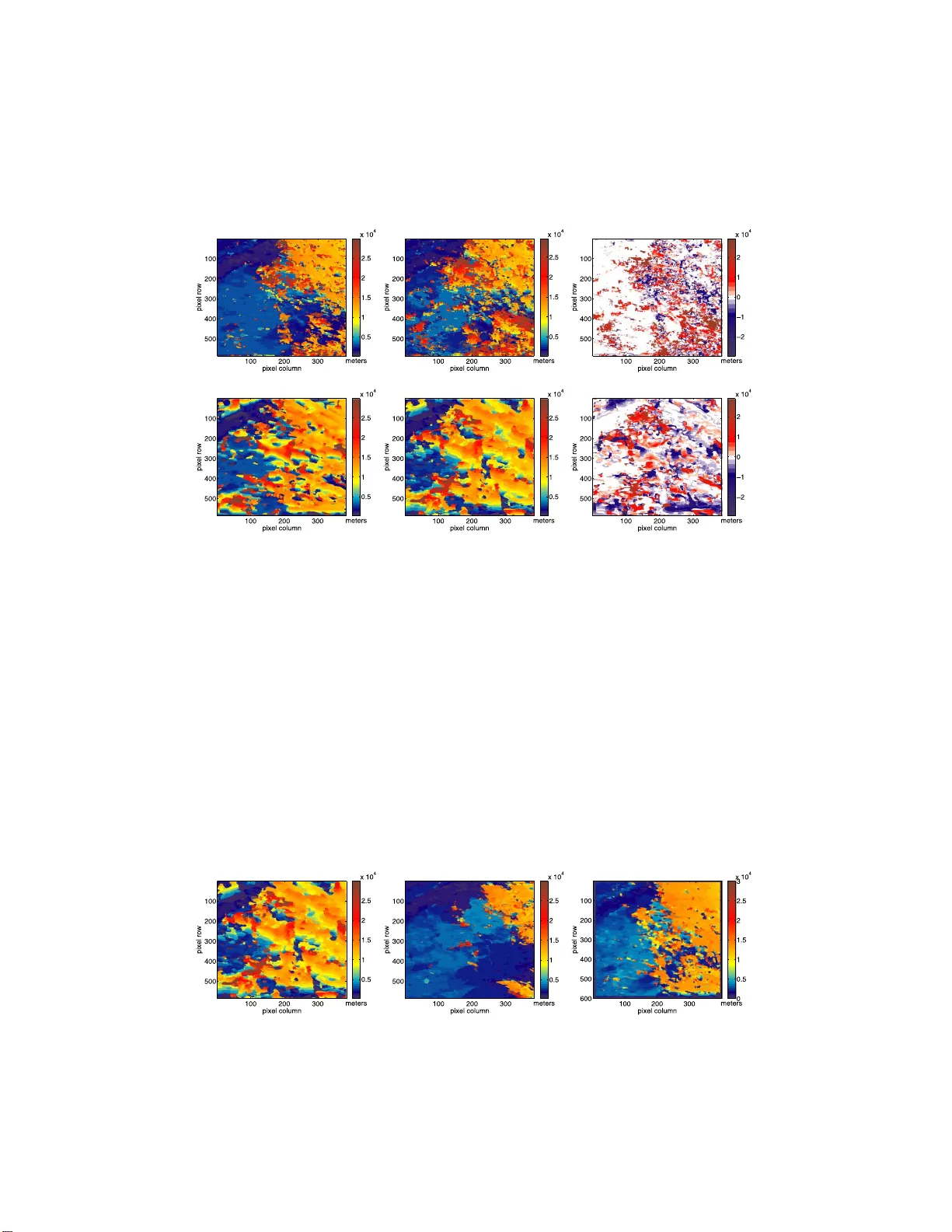
The Annals of Applie d Statistics 2009, V ol. 3, No. 3, 902–921 DOI: 10.1214 /09-A OAS243 In th e Publi c Domain MAXIMUM LIKELIHOOD ESTIMA TION OF CLOUD HEIGHT FR OM MUL TI-ANGLE SA TELLITE IM A GER Y By E. Anderes 1 , B. Yu 2 , V. Jov ano vic, C. Moroney, M. Gara y, A. Bra verman and E. Clothia ux University of California at Davis, U ni v ersity of California at Berkeley, California Institute of T e chnolo gy, California Institute of T e chnolo gy, R aythe on Corp or ation, California Institute of T e chnolo gy and Pennsylvania State U niversity W e develop a new estimatio n technique for recov ering dep t h-of- field from multiple stereo images. Dept h -of-field is estimated by de- termining t he shift in image location resulting from different cam- era viewpoints. When this shift is not divisible b y pixel width, the multiple stereo images can b e com b ined to form a super-resolution image. By mo deling th is sup er-resolution image as a realization of a random field, one can view the recov ery of dep th as a lik elihoo d estimation problem. W e apply these mo deling tec hn iques to the re- co very of c loud heigh t from m ultiple viewing angles provided by th e MISR i nstrument on the T erra S atellite. O ur efforts are focused on a t wo laye r c loud ensem ble where both la yers a re relativ ely planar, the bottom lay er is optically thick and textured , an d th e top l a yer is optically thin. Our results demonstrate that with relative ease, we get comparable estimates to the M2 stereo matcher whic h is the same algorithm used in the current MISR standard pro duct (details can b e found in [ IEEE T r ansactions on Ge oscienc e and R emote Sensing 40 (2002) 1547–15 59]). Moreov er, our techniques p ro v ide t he p ossibilit y of modeling all of the M ISR data in a unified wa y for cloud height estimation. Researc h is underwa y to extend this framew ork for fast, quality global estimates of cloud h eigh t. 1. In tro d uction. The motiv ation for this p ap er comes from the problem of reco vering cloud heigh t from the Mu lti-Angle Imaging Sp ectroRadiometer Received May 2008; revised March 2009. 1 Supp orted in part by an NSF P ostdo ctoral F ellowship DMS- 05-03227 and JPL Grant 1302389 . 2 Supp orted in part by Grants N SF DMS-06-05165, ARO W911NF-05-1-0104, NSFC- 6062810 2, a Guggenheim F ello wship in 2006 and a grant from MSRA. Key wor ds and phr ases. Random fi elds, cloud heigh t estimation, sup er resolution, mul- tiangle imaging sp ectroradiometer, depth- of-field, maxim um likel ihoo d estimation. This is an electronic reprint o f the o riginal article published by the Institute of Mathematical Statistics in The Annals of A pplie d S tatistics , 2009, V ol. 3, No. 3, 902– 921 . This repr int differs from the original in paginatio n and t y po graphic detail. 1 2 E. AN DERES ET AL. (MISR) in s trument , laun c hed in Decem b er 1999 on the NASA EOS T erra Satellite. Clouds pla y a ma jor role in determining th e Earth ’s energy b ud- get. As a result, monitoring and charac terizing the d istribution of clouds b ecomes imp ortan t in global studies of climate. T he MISR instru men t pro- duces images (275 m r esolution) in the red band o ver a swath width of 360 km for n ine camera angles: 70 ◦ , 60 ◦ , 45 . 6 ◦ , 26 . 1 ◦ forw ard angles, a nadir view at 0 ◦ , and aft angles 26 . 1 ◦ , 45.6 ◦ , 60 ◦ , 70 ◦ (referred to as Df, Cf, Bf, Af, An, Aa, Ba, Ca and Da resp ectiv ely). By taking adv antag e of the image displacemen t that results fr om multi-angle image geometry , one can r eco v er cloud top heigh t and cloud motion (where cloud motion is determined from wind). Unfortunately , tr ansparency , m ultiple la ye rs, o cclusion and heigh t discon tinuities p resen t c h allenges for cloud h eigh t estimation. In this pap er w e apply new statistical tec h niques for estimating cloud heigh t and attempt to reco ver cloud heigh t for a t w o la ye r ensemble: an optically thin top la y er o ve r a textured b ottom la yer. The image d isp lacemen t that results from ground registration is, almost alw a ys, not divisible by the p ixel width. By taking adv antag e of this offset, one can construct a sup er-resolution image fr om the different viewing angles. It is this su p er-resolution image that w e mo del as a discrete samp le from a realizatio n of a contin uous Gaussian r andom field. Under this p aradigm, es- timating h eigh t and wind can b e view ed as a statistical likeli ho o d estimation problem. T here are seve ral adv antag es of this ap p roac h. First, by c hanging the mo del of the late nt con tinuous image, one ca n c h ange the matc hing c haracteristics of th e algorithm and, p oten tially , optimize th e matc hin g for differen t cloud ensem b les. Second, the sup er-resolution framework extend s naturally when there are more than t wo camera angles. Finally , the mo d eling of the sup er-resolution im age giv es a u nified wa y of estimating sub-grid-scale displacemen t. There is a considerable amoun t of existing literature on b oth the reco very of thr ee dimensional stru cture from m u ltiple stereo images and constru cting sup er-r esolution images from m ultiple stereo images. The literature on b oth problems is v ast and sp an s o v er at least 20 years. W e refer r eaders to t wo re- views, Bro w n, Burs chk a and Hager ( 2003 ) and Dhond and Aggarw al ( 1989 ), on the reco v ery of d epth-of-field and t wo reviews, F arsiu et al. ( 2004 ) and P ark, P ark and Kang ( 2003 ), on the su p er-resolution problem. T o the au- thors’ kno w ledge, the tw o problems ha ve yet to b e considered concurrently for reco very of d epth-of-field which is the fo cus of the current pap er. The rest of the p ap er is organized as follo ws. In Section 2 we describ e our new tec hniqu e for estimating depth-of-field from m ultiple images taken from differen t viewp oints. In Section 3 we s ho w how to use this sup er-resolution framew ork for estimating cloud h eigh t from th e MISR data. Finally , S ection 4 presents our test results for cloud height estimation. MAXIMUM LIKELIHO OD ESTIMA TION OF CLOUD H EIGHT 3 2. The sup er-resolution likelihoo d. In this section we describ e our tec h- nique for reco ve ring depth -of-field from multiple stereo images. W e start with our notation for non u n iformly sampled images and fin ish with a pr esen tation of our n ew estimation metho d ology that u ses sup er-resolution tec hniques and rand om field mo d els to define a lik eliho o d for estimating depth-of-field. This exp osition is done as general as p ossible to av oid letting the details of the cloud heigh t problem obstruct the general estimation p ro cedure (the details of the cloud height estimation are then p resen ted in S ection 3 ). 2.1. Image notation. Even though it is easy to visualize the construc- tion of a sup er-resolution image, the mathematical notation to express this construction is somewhat clum s y . Th e basic ob ject for our notation is an image, denoted ( x , y ). The p ixel locations are enco ded in the order ed list of spatial co ord inates x and the corresp onding gra y v alues, or radiances, are enco ded in the v ector y . In the regression setting, one might consider x to b e a m atrix w ith t wo columns wh ere eac h ro w is a pixel lo cation. How ev er, w e prefer to use the ‘list’ charact erization so that, for example, a fu n ction f : R 2 → R ev aluated at a list of lo cations x , denoted f ( x ), will represent comp onent -wise ev aluation of f on e ac h elemen t of the list (rather than ro w-wise ev aluation u sing the regression notation). In this w ay , shifting all the spatial lo cations in x by the same δ ∈ R 2 can b e written x + δ . The pixel lo cations x allo w u s to define n on un iformly sampled images. Therefore, when wo rking with o ne ima ge, x serv es to sp ecify the o verall structure of the image. When wo rking with m ultiple images, the ind ivid- ual pixel lo cations ma y b e useful for comparing lo cations a cross multi- ple images. F or example, if one has n images on a square grid of equal size, it ma y mak e se nse to se t the l o wer left pixel at the origin, all with the same pixel spacing. Mu ltiple images will b e written with sup erscripts ( x (1) , y (1) ) , . . . , ( x ( n ) , y ( n ) ), reserving sub scripts to denote the element s of a list. In particular, x j and y j denotes the j th pixel an d the corresp onding j th gra y v alue or radiance. F or example, a 2 × 2 gra y lev el image could b e wr it- ten x = ((0 , 0) , (0 , 1) , (1 , 0) , (1 , 1)) , y = (0 . 4 , 0 . 2 , 0 . 1 , 0 . 7) T so that the s econd pixel has co ord in ates x 2 = (0 , 1) with gra y v alue y 2 = 0 . 2. No w the sup er-resolution image is defined b y direct concatenatio n of the pixel lo cations and th e gray v alues. In particular, le t ( x (1) , y (1) ) and ( x (2) , y (2) ) b e t w o images whic h we wan t to o v erla y to constru ct a s u p er- resolution image. The in tuition is that these tw o images a re of t he same physic al ob ject b ut pro jected on d ifferen t pixel grids (see Figure 1 ) . The sup er-r esolution image is defined as (  x (1) x (2)  ,  y (1) y (2)  ). It ma y b e th e situation that the fir st image ( x (1) , y (1) ) needs to b e shifted by some vect or δ ∈ R 2 b e- fore it is o v erlaid with the second image ( x (2) , y (2) ). T he pr o cess of shifting the first image by δ then o verla yin g the tw o to construct a sup er-resolution image is wr itten (  x (1) + δ x (2)  ,  y (1) y (2)  ). 4 E. AN DERES ET AL. Fig. 1. An il lustr ation of the c onstruction of the sup er-r esolution i m age ( x , y ) . T he obje ct c aptur e d by ( x (1) , y (1) ) shifts to ( x (2) , y (2) ) in the next c amer a angle. If the p ar al lax is known and is not a multiple of the grid sp acing, the two image p atches c an b e overlaid to cr e ate a sup er-r esolution image. 2.2. Su p er-r esolution, r andom fields and depth-of-field. W e start with n images, eac h rep r esen ting different pictures of the s ame ob j ect take n from n differen t camera viewp oints (see the first illustration of Figure 2 ). Sin ce the cameras are fr om d ifferent viewp oints, th e ob ject will app ear in differen t image l o cations in eac h camera (see the second i llustration of Figure 2 ). W e defin e p ar al lax as the difference in image lo cation of the ob ject in eac h camera. Notice th at once the geometry of the camera configuration is fixed, Fig. 2. An il lustr ation of the distanc e p ar ameter d and p ar al lax. Onc e the ge ometry of the c amer a arr ay i s fixe d, the p ar ameter d c ompletely determines the p ar al lax. MAXIMUM LIKELIHO OD ESTIMA TION OF CLOUD H EIGHT 5 the parallax is completely characte rized by the distance, d , of the ob ject to one of the cameras. Typical estimation of d (i.e., dep th -of-field) amounts to estimating the parallax of the ob ject b et ween eac h pair of cameras then u sing these parallaxes to solv e for d . Our metho d, on the other h and, estimates d dir ectly , treating it as an unkn own statistical parameter. Th e adv anta ge is that d completely c haracterizes the parallax observed b et ween eac h pair of cameras, thereb y reducing th e p roblem to estimating a single parameter and mo deling the observ ations jointl y rather than pairw ise. In more detail, consider a physical ob ject captured in the image patc h ( x (1) , y (1) ) and let d ∈ (0 , ∞ ) denote the distance of this ob ject to the fir st camera. As one v aries d , there will exist different image patc hes ( x (2) , y (2) ) , . . . , ( x ( n ) , y ( n ) ) from the subsequent camera angles, all of which capture the ob- ject ap p earing in ( x (1) , y (1) ). This implies the existence of shifts δ 2 , . . . , δ n so that the n ew sup er-resolution image, ( x , y ), giv en by x :=      x (1) x (2) + δ 2 . . . x ( n ) + δ n      , y :=    y (1) . . . y ( n )    , (1) is a picture of the same ob ject captured by ( x (1) , y (1) ) (see Figure 1 ). Note that the shifts δ 2 , . . . , δ n and the image patc hes ( x (2) , y (2) ) , . . . , ( x ( n ) , y ( n ) ) dep end solely on the distance parameter d . W e call the pro cess of combining image patc h es to constru ct a su p er-resolution image “inte r lacing.” T o co mpute a lik eliho o d for estimat ing the p arameter d , we start b y supp osing there exists a laten t contin uous function Y : R 2 → R that m o d- els the co n tinuous image in the lo cal patc h ( x (1) , y (1) ). In ot her w ords, Y ( x (1) ) = y (1) . Note that Y ( x ) denotes the list obtained b y ev aluating Y at eac h p ixel lo cation in the list x . F or the tr ue distance p arameter d , the sup er-r esolution image ( x , y ) will also satisfy Y ( x ) = y . The w rong distance parameter will i n terlace imag es of differen t regions whic h will resu lt in a ‘noisy’ sup er-r esolution image for w hic h it w ill b e d ifficult to find a contin- uous in terp olator that satisfies Y ( x ) = y . By putting a p robabilit y m easure P on the laten t contin uous image Y , w e can estimate the distance of the ob ject b y minimizing the follo wing negativ e log like liho o d: − ℓ ( d ) := − log P ( Y ( x ) = y ) , (2) where the su p er-resolution image ( x , y ), dep ending on d , is constructed as in ( 1 ). An equiv alen t wa y to sp ecify the log- lik eliho o d ( 2 ) is to simply clai m that there exists image patc hes ( x (2) , y (2) ) , . . . , ( x ( n ) , y ( n ) ) and lo cation shifts δ 2 , . . . , δ n , all dep ending on the parameter d , such that Y ( x (1) ) = y (1) and y ( k ) = Y ( x ( k ) + δ k ) , k = 2 , . . . , n. (3) 6 E. AN DERES ET AL. Since Y do es not dep end on k in the ab o v e equation, the sup er-resolution image defin ed by ( 1 ) satisfies y = Y ( x ). Ther efore, un der the mo del P , the join t distribution of y is the s ame as that obtained in ( 2 ). This alternativ e w ay of expressin g the sup er-resolution lik eliho o d will b ecome u seful in the follo wing sections for in tro ducing nuisance p arameters asso ciated w ith the MISR cameras. 3. Cloud heigh t estimation. This section contai ns the m o deling details for cloud height estimation from MISR satellite data. In our view, one of the adv anta ges of the estimation techniques outlined in the previous section is th e ease in whic h the tec hnical details of a particular observ ation scenario can b e incorp orated into the reco ve ry of depth-of-field. W e d emonstrate this flexibilit y in our ap p lication of this metho d ology to cloud heigh t estimation. This section starts with a discuss ion of the relationship b et wee n parallax, cloud heigh t and wind. S ection 3.1 present s a summary of all the m o deling assumptions used to compu te the m axim um like liho o d estimation of height . A more thorough explanation of th e mo d eling assum ptions and the tec h- niques for co mputing t he like liho o d c an b e found in Secti ons 3.1.1 , 3.1.2 and 3.1.3 . F or the MISR data, instead o f estimating distance to the satellite, w e w ant to estimate cloud heigh t and w ind. Since the parallax of a cloud patc h is completely determined b y h eight and wind, the tec hniqu es from Section 2 are easily app licable. Indeed, one of the main features of the metho dology dev elop ed in the last section is that it r elates all the observ ed parallaxes to a single parameter d . In the MISR data, the parameter d , that is, distance of the ob ject to the satelli te, is directly related to cloud height (since the heigh t of a cloud determines the distance to the satellite). Ho wev er, there is an ad d ed complication of cloud mov ement as a fun ction of w ind. S ince wind will a lso effect the image lo cation of a cloud in eac h camera, w e includ e it as a paramete r so that no w h eigh t h and a win d v elo cit y v := ( v 1 , v 2 ) completely d etermine parallax and the constru ction of the sup er-resolution image ( x , y ). F or the MIS R images there is an appro ximate linear r elationship th at relates w in d, cloud height and image parallax. Let t ( k ) denote the fl y-o ve r time dela y (in seconds) for th e k th camera and x ( k ) the along-trac k image lo cation of a lo cal cloud region in camera image k . When h is in meters, v is in meters p er second, and th e p ixel lo cations sp ecified b y x ( k ) all repr esen t the s ame 275 meter grid, th e linear equation that relates w ind, heigh t and along-trac k parallax are v 2 ( t ( i ) − t ( j ) ) + h (tan( θ ( i ) ) − tan( θ ( j ) )) = x ( i ) − x ( j ) , (4) where θ ( k ) is th e angle of eac h camera. The across-trac k parallax is giv en b y v 1 ( t ( i ) − t ( j ) ). F or more details see Diner et al. ( 1997 ). MAXIMUM LIKELIHO OD ESTIMA TION OF CLOUD H EIGHT 7 Before w e con tin ue, w e men tion th at since clouds b ehav e dy n amically there is the p ossibilit y of a c h an ge in cloud structur e within the time dela y of the different cameras. Ho wev er, since this dela y is at m ost 7 m inutes (the appro ximate dela y from the Df camera to the Da camera) and the pixel patc hes we will b e using corresp ond to ab out 4 squ are kilometers (15-b y-15 pixel patc hes), we will tacitly assu me this effect is negligible. 3.1. D etaile d summary of the mo del. A ma j or obstacle in usin g the meth- o ds in S ection 2 f or the MISR data is th at the images f rom different angles often hav e d ifferent o ve rall brightness. Therefore, it b ecomes d ifficult to d i- rectly interla ce patc hes from d ifferen t images. In what follo ws w e mo del this brigh tness c h ange as a linear correction for eac h camera. Supp ose the image patc h ( x (1) , y (1) ) captures a small cloud region and let Y b e the con tinuous r ep resen tation of this image so that Y ( x (1) ) = y (1) . The true h eigh t and wind, ( h, v ) , allo w us to retriev e patc hes ( x (2) , y (2) ) , . . . , ( x ( n ) , y ( n ) ) from the subsequent camera angles, eac h c apturing the same cloud region p ro jected on p oten tially shifted grids. F or the remainder of the pap er, n denotes the n umb er of cameras and m d enotes the num b er of pixels in eac h p atc h ( x ( k ) , y ( k ) ), k = 1 , . . . , n . Our m o del for the gra y v alues y ( k ) is summarized by y ( k ) = σ k Y ( x ( k ) + δ k ) + A k x ( k ) + b k (5) for cameras k = 2 , . . . , n , w here • Y is the l aten t contin uous cloud image, mo deled b y a Gaussian ran- dom fi eld with Mat ´ ern co v ariance function K with parameters ( σ, ρ, ν ) = (1 , 4 , 4 / 3) (see S ection 3.1.1 ) so that co v ( Y ( t ) , Y ( s )) = K ( | t − s | ) , for all t , s ∈ R 2 where | · | d enotes Euclidean distance; • σ k is a multiplica tiv e b r igh tness correction for eac h camera; • δ k is a t wo dimensional s h ift ve ctor which is completely determined by ( h, v ) and pla ys th e role of sh ifting the pixel lo cations x (1) , . . . , x ( n ) so that they are int erlaced; • A k is a 2 × 1 matrix whic h repr esents an affine b righ tn ess correction for eac h patc h ; • b k is an ov erall constant additiv e correction. Notice that Y mo dels th e laten t cloud image for eac h camera so we obtain a join t mo d el for the fu ll sup er-resolution vect or y := ( y (1) T , . . . , y ( n ) T ) T . By the Gaussian assum ption on Y , we ha ve y ( k ) ∼ N ( A k x ( k ) + b k , σ 2 k Σ k ) , (6) where Σ k := ( K ( | x ( k ) i − x ( k ) j | )) ij . 8 E. AN DERES ET AL. Since we h a ve intro d uced an additiv e and multiplic ativ e br igh tness cor- rection on eac h patc h, it is no longer tru e that the sup er-resolution image satisfies y = Y ( x ), where x is defined by ( 1 ). What is t rue, ho wev er, is that y = diag( σ 1 I m , . . . , σ n I m ) Y ( x ) + µ , w here µ is a v ector with k th blo c k A k x ( k ) + b k and I m is the m × m iden tit y matrix. Th e m ain difficu lty for es- timation of ( h, v ) no w b ecomes devising tec h niques for d isp ensing with the n u isance p arameters σ k , A k , b k . This is the main con tribution of Sections 3.1.2 and 3.1.3 . Both sections us e REML techniques [see Stein ( 1999 )] to filter out the additiv e b righ tness corrections A k x ( k ) + b k . Dealing with th e m u ltiplicativ e nuisance parameters σ k is more difficult and requires separate treatmen ts f or high and low clouds. F or high clouds, a brightness stabiliza- tion allo ws u s to marginalize out σ k . F or lo w clouds, th ere is no closed form solution for the marginalized lik eliho o d a nd w e resort to an app ro ximate profile lik eliho o d. Remark. The affine corr ection A k x ( k ) + b k , rather than a higher ord er p olynomial, was c h osen for tw o r easons. First, the size of th e pixel p atc h is relativ ely small. S mall enough, in fact, so that on e might exp ect a linear T a ylor app ro ximation to b e v alid. Seco nd, a linear p olynomial seems th e natural choic e for a once, bu t n ot t w ice, differen tiable cloud pro cess, wh ic h is derived in th e follo win g su bsection. 3.1.1. G aussian r andom field mo del for P . In ( 5 ) we u s e a Mat ´ ern auto- co v ariance function K [with p arameters ( σ, ρ, ν ) = (1 , 4 , 4 / 3)] to mo del the co v ariance structure of the laten t con tinuous cloud image Y . This section outlines our motiv ation for our c hoice of the Mat ´ ern autoco v ariance fu nction and the sp ecific parameter v alues. The basic id ea is to use the observ ed frac- tal b ehavi or of clouds [see Cahalan and Snid er ( 1989 ), Bark er and Da vies ( 1992 ), V´ a rnai ( 2000 ), Oreop oulos et al. ( 2000 ) and Da vis et al. ( 1997 ) from the atmospheric science literature] to mo del the fractal nature of Y after ad- justing for pixel a veraging. Indeed, one of the adv an tages of the the Mat ´ ern auto co v ariance f u nction is the flexibilit y it provides for mo d eling the fr actal b ehavi or of Y . The Mat ´ ern auto co v ariance fu nction K is defined by K ( r ) = σ 2 ν − 1 Γ( ν )  2 ν 1 / 2 r ρ  ν K ν  2 ν 1 / 2 r ρ  , where K ν is the mo d ified Bessel function [see Stein ( 1999 )]. W e mo del Y , the con tin u ou s cl oud image, as a t wo dimensional Gaussian random field with co v ariance structure giv en by co v ( Y ( s ) , Y ( t )) = K ( | s − t | ) for all s, t ∈ R 2 with parameters ( σ, ρ, ν ) = (1 , 4 , 4 / 3). The parameter σ is the v ariance v ar[ Y ( t )] at any fi xed p oint t ∈ R 2 . The parameter ρ serv es as the range MAXIMUM LIKELIHO OD ESTIMA TION OF CLOUD H EIGHT 9 parameter for Y so that co v ( Y ( s ) , Y ( t )) quickly b ecomes negligible when the lag | s − t | is larger than ρ . T he ν parameter controls the smo othness of the pr o cess. In our analysis the r ange p arameter ρ is set to 1100 meters (4 p ixel w idths) and th e v ariance p arameter σ is 1. With the exception of either very sm all or very large ρ , different v alues of ρ , σ do not sev erely e ffect o u r height estimates. In the case of v ery large ρ it seems that the lo cal pat c h size b ecomes to o small, compared to the range, for appr opriate mo deling. When ρ is very small, the estimation of heigh t and wind b ecomes ineffectiv e since most of th e in terlaced images are m o deled as n early uncorrelated. Here w e derive our justification for ν = 4 / 3 as a plaus ib le v alue for the smo othness parameter. In our analysis, the v ector y ( k ) represent s the log of registered bidirectional r eflectance factor (BRF) v alues from the k th camera. Let I BRF denote the laten t con tinuous BRF image so that Y = log ( ϕ ∗ I BRF ), where the pixelation is represen ted by the con vo lu tion ke rnel ϕ = I [ − 1 / 2 , 1 / 2] 2 for the in dicator function I . Let K BRF b e the auto co v ariance fun ction for the cont in u ous BRF image I BRF . The tw o d imensional F ourier transform of K BRF giv es th e sp ectral densit y f I BRF ( ω ) := 1 (2 π ) 2 Z R 2 exp( − ix T ω ) K BRF ( x ) dx, where x = ( x 1 , x 2 ) and ω = ( ω 1 , ω 2 ) are b oth t wo dimensional vecto r s. There is evidence to suggest that K olmogoro v’s 5 / 3 sc aling la w h olds for f I BRF [see Cahalan and Snider ( 1989 ), Bark er and Da v ies ( 1992 ), V´ arnai ( 2000 ), Oreop oulos et al. ( 2000 ) an d Da vis et al. ( 1997 )]. Und er the additional as- sumption of isotrop y , the scaling la w implies th e t wo dimens ional sp ectral densit y satisfies f I BRF ( ω ) ≍ 1 | ω | 5 / 3+1 as | ω | → ∞ . Therefore, the sp ectral den- sit y of the pixelated pr o cess ϕ ∗ I BRF is giv en by f ϕ ∗ I BRF ( ω ) = | ˆ ϕ ( ω ) | 2 f I BRF ( ω ) ≍ sinc 2  ω 1 2  sinc 2  ω 2 2  1 | ω | 5 / 3+1 , (7) as | ω | → ∞ . Let f Y denote the sp ectral density for the Mat ´ ern auto co v ari- ance mo del for Y . W e b eliev e a p lausible v alue for the parameter ν , for the random field Y = log ( ϕ ∗ I BRF ), corresp ond s to matc hing the p o wer-la w de- ca y of f Y to that of f ϕ ∗ I BRF , in the co ordinate directions. I n p articular, by ( 7 ) and the prop erties of th e Mat ´ ern sp ectral densit y , f ϕ ∗ I BRF ( ω ) ≍ sin 2 ( ω 1 / 2) | ω 1 | 5 / 3+3 , f Y ( ω ) ≍ 1 | ω 1 | 2 ν +2 , fixing ω 2 and letting ω 1 → ∞ . Therefore, to matc h the deca y , w e set the smo othness parameter ν to (5 / 3 + 1) / 2 = 4 / 3. 10 E. AN DERES ET AL. 3.1.2. L ow-cloud likeliho o d. Here w e giv e some of the computational tec h - niques for dealing with the n u isance parameters when estimating the heigh t of lo w textured clouds. W e start b y constru cting a matrix L (‘ L ’ for lo w ) whic h fi lters out the dep endence of the obser v ations on A k and b k . T h en w e constru ct an approximat e p rofile like liho o d to handle the multiplica tiv e n u isance parameters σ k . F or lo w textured clouds we b egin b y constru cting n matrices L 1 , . . . , L n whic h annihilate monomials of order at most 1 so that L k y ( k ) ∼ N (0 , σ 2 k Σ k ). In particular, L k is a ( m − 3) × m matrix with ro ws comp osed of linearly in de- p endent vec tors in th e k ern el space { v : [ φ 0 ( x ( k ) ) φ 1 ( x ( k ) ) φ 2 ( x ( k ) )] T v T = 0 } , where φ 0 , φ 1 and φ 2 are the the mon omials of order at m ost 1. No w define the ma trix L = diag ( L 1 , . . . , L n ) so that L y ∼ N (0 , ∆ σ ˜ Σ∆ σ ), where ˜ Σ := L Σ L T , Σ := ( K ( | x i − x j | )) ij and ∆ σ := diag ( σ 1 I m − 3 , . . . , σ n I m − 3 ). There- fore, the lik eliho o d of the observ ation v ector L y , as it dep ends on ( h, v ) and σ := ( σ 1 , . . . , σ n ) T , can b e written L ( h, v , σ | L y ) = 1 | 2 π ˜ Σ | 1 / 2 1 | ∆ σ | exp  − 1 2 ( L y ) T ∆ − 1 σ ˜ Σ − 1 ∆ − 1 σ ( L y )  . A t this p oint there are a few options to disp ense with the dep endence of the ab ov e likelihoo d on the n uisance parameters σ . Th e most desirable op- tion would b e to marginalize ou t σ by in tegrating R R n + L ( h, v , σ | L y ) d σ . F or eve n mo derate blo c k s ize m and n = 2, this b ecomes computationally formidable. Th e second option w ould b e to maximiz e a profile likelihoo d L ( h, v | L y ) := m ax σ ∈ R n + {L ( h, v , σ | L y ) } . Th is option is somewhat more com- putationally tractable b u t still problematic since there is n o closed form for the profile lik eliho o d. The easiest option is to estimate σ k on eac h patc h sep- arately , ˆ σ 2 k := ( L k y ( k ) ) T ( L k Σ k L T k ) − 1 ( L k y ( k ) ) /m , then maximizing a p lug-in v ersion of the likeli ho o d L ( h, v , ˆ σ | L y ), where ˆ σ := ( ˆ σ 1 , . . . , ˆ σ n ) T . Notice, ho wev er, that u nder the correct ( h, v ) the patc h es y (1) , . . . , y ( n ) are highly correlated, and, therefore, in formation is lost b y estimating σ k separately on eac h p atch. In an attempt to alleviate this problem, w e explore a compro- mise b et w een the full pr ofile lik eliho o d and th e ov erly simp listic case of the plug-in lik eliho o d with ˆ σ . Notice that the quadratic term ( L y ) T ∆ − 1 σ ˜ Σ − 1 ∆ − 1 σ ( L y ) can b e written k ˜ Σ − 1 / 2 ∆ − 1 σ L y k 2 =     R 1 L 1 y (1) σ 1 + · · · + R n L n y ( n ) σ n     2 = σ − T ˜ R σ − 1 , where the m atrices R 1 , . . . , R n decomp ose ˜ Σ − 1 / 2 in to blo ck f orm so that ˜ Σ − 1 / 2 = ( R 1 , . . . , R n ) and ˜ R is the mat rix of inner pro du cts ( h R i L i y ( i ) , R j L j y ( j ) i ) ij . Ther efore, the log lik eliho o d can b e w ritten ℓ ( h, v , σ | L y ) = c 1 − 1 2 log | ˜ Σ | − ( m − 3) n X k =1 log σ k − 1 2 σ − T ˜ R σ − 1 , MAXIMUM LIKELIHO OD ESTIMA TION OF CLOUD H EIGHT 11 where c 1 is a constant. F or a fi xed ( h, v ) , m aximizing ℓ ov er σ is a con ve x problem whose stationary p oin t is c h aracterized by ˜ R σ − 1 − ( m − 3) σ = 0 . (8) This equation d efines the pr ofi le likeli ho o d but unfortu nately h as no closed form solution for general n . Ho wev er, there is considerable research on in v es- tigating iterativ e algorithms for solving ( 8 ) [see Marshall and O lkin ( 1968 ), Khac h iyan and K alan tari ( 1992 ) a n d O’Leary ( 2003 ), f or e xample]. The problem with iterativ e algorithms is that th e lik eliho o d compu tation will b e done man y times wh ile sea rc hin g through heigh t and wind o ver slid- ing blo c ks. Therefore, including an iterativ e al gorithm in the like liho o d calculatio n pr esen ts some compu tational problems. As a compromise, w e define a “one Newton step” estimate of th e stationary p oin t of ( 8 ) with an initial starting point ˆ σ , the maxim um like lih o o d estimate q ( L k y ( k ) ) T ( L k Σ k L T k ) − 1 ( L k y ( k ) ) /m from eac h camera separately . The Newton step is constructed as in Khac hiy an a nd K alanta ri ( 1992 ) and d efined for σ − 1 rather than σ . In p articular, d efine F ( σ − 1 ) = ˜ R σ − 1 − ( m − 3) σ and ˜ ∆ σ := diag( σ 1 , . . . , σ n ). No w F ( σ − 1 + τ ) = F ( σ − 1 ) + ˜ R τ + ( m − 3) ˜ ∆ 2 σ τ plus h igher order terms in τ . Setting th is linear appro ximation to zero and solving for τ gi v es the Newton step σ − 1 + τ . W e use the initial starting p oint ˆ σ − 1 . Notice th e Newton step may r esult in a negativ e v ariance, in which case, the original estimate ˆ σ is used instead of the Newton step. In summ ary , to estimate ( h, v ), we define the “one Newton step” ( ˆ σ newton ) − 1 :=      ˆ σ − 1 + ( ˜ R + ( m − 3) ˜ ∆ 2 ˆ σ ) − 1 (( m − 3) ˜ ∆ 2 ˆ σ − ˜ R ) ˆ σ − 1 , if p ositiv e; ˆ σ − 1 , otherwise , and maximize the plug-in log-lik eliho o d \ ( h, v ) := arg m ax ( h, v ) ℓ ( h, v , ˆ σ newton | L y ) . 3.1.3. High-cloud likeliho o d. Here w e giv e some of the computational tec hniques fo r dealing with the n uisance p arameters when estimating the heigh t of high thin clouds. S in ce these heights are notoriously hard to esti- mate, we attempt a brigh tness stabilization on th e whole cloud image wh ich allo ws m ore lo cal inform ation for estimating c loud heigh t. After th is sta- bilization, w e construct a matrix H (‘ H ’ is for high) whic h filters out th e common v alue of the stabilized n uisance parameters A k and b k . F or the brigh tness corrections σ k , our s tabilizatio n allo ws us to marginalize out the common v alue of σ k under a unif orm prior w hic h is far more desirable than the appr o ximate pr ofile likelihoo d techniques needed for low cloud s . 12 E. AN DERES ET AL. One of the difficulties of high clo uds is that they are frequentl y opti- cally t hin or p artially transp aren t. This mak es estimating parallax diffi- cult b ecause the dominan t signal is frequently th e b ackg round r ather than the c loud itself. In an a ttempt to o verco me this difficult y , w e estimate a linear transformation on y ( k ) for eac h camera k = 1 , . . . , n to stabilize the brigh tness corr ections m o deled b y σ k , A k and b k . A more in-depth d iscus- sion on this issue is p resen ted in S ection 4 . Once s tabilizati on is ac hieved, w e ha ve y ∼ N ( A x + b, σ 2 Σ), where σ, A and b are the common v alues of σ k , A k and b k resp ectiv ely and Σ := ( K ( | x i − x j | )) ij . T his allo ws us to fi nd a matrix H for whic h H y ∼ N ( 0 , σ H Σ H T ). H is defined as the matrix with ro ws co mp osed of linearly indep en d en t v ectors in the k ern el sp ace { v : [ φ 0 ( x ) φ 1 ( x ) φ 2 ( x )] T v T = 0 } . Notice that no w H is not blo c k d iagonal as it was for L . As a consequence, H y is a vecto r of length nm − 3 ve rsus ( m − 3) n (for the lo w cloud estimates), wh er e n and m denote the num b er of cameras and p atc h size r esp ectiv ely . This provides more inform ation for matc hing in an attempt at r eco v er in g th e high-cloud heights. The lik eliho o d of h, v and σ , giv en the observ ation vec tor H y , h as the follo wing form: L ( h, v , σ | H y ) = 1 σ nm − 3 | 2 π ˜ Σ | 1 / 2 exp  − y T H T ˜ Σ − 1 H y 2 σ 2  , where ˜ Σ := H Σ H T . In cont rast with the lo w-cloud likeli ho o d, w e can remov e the dep end ence on the un kno w n parameter σ by m arginalizing out u nder a uniform improp er p rior L ( h, v | H y ) ∝ Z R + L ( h, v , σ | H y ) dσ = 2 ( nm − 4) / 2 2 | 2 π ˜ Σ | 1 / 2 Γ(( nm − 4) / 2) [ y T H T ˜ Σ − 1 H y ] ( nm − 4) / 2 . The in tegral is obtained b y the c hange of v ariables x = σ 2 and recognizing an un-normalized inv erse gamma density . Therefore, the log-lik eliho o d whic h is maximized o ver ( h, v ) is ℓ ( h, v | H y ) = c 2 − 1 2 log | ˜ Σ | − nm − 4 2 log[ y T H T ˜ Σ − 1 H y ] , (9) for some constant c 2 . Remark. Instead of marginalizing out the un kno wn σ , one could in - stead m aximize a profile log-lik eliho o d as a fu nction of ( h, v ) , where the profiling is ov er the unk n o wn σ . The resulting profile log-lik eliho o d is c 3 − 1 2 log | ˜ Σ | − nm − 3 2 log[ y T H T ˜ Σ − 1 H y ] w hic h, it app ears, fails to tak e into ac- coun t the loss of degrees of freedom asso ciated with the un kno wn σ . MAXIMUM LIKELIHO OD ESTIMA TION OF CLOUD H EIGHT 13 3.1.4. Simula tion study. Before our method ology is applied to the MISR data, w e present a s hort simulatio n study that provides some evidence that the appr o ximations used in the ab o ve metho d ology are n ot only v alid in some cases b ut can also pro vide an impro vemen t o v er the M2 algorithm. Although our simulations provide fa vo rable evidence for our metho dology , we b eliev e the rea l strength lies in its flexibilit y to incorp orate st atistical principles and science to the problem of cloud height r etriev al. Before w e con tin ue, we stress that this simulat ion is designed to test th e m atc hing algorithm wh en the probabilistic mec hanism that generates the cloud images is known. In general, this w ill n ot b e the case. Therefore, we consider simulati ons of this t yp e to b e one comp onen t of a full in v estigation of the p oten tial for the sup er-r esolution metho dology . W e ha ve three main ob jectiv es for our sim ulations. The first is to sho w that one can obtain go o d cloud-heigh t estimates by correctly sp ecifying the high fr equency b eha vior of th e sp ectral density (as we do in Section 3.1.1 ) ev en when the the lo w frequency b eha vior is m is-sp ecified. Second, w e will argue that the join t mo deling of the full sup er-resolution image, rather than pairwise mo d eling f or eac h camera, giv es b etter estimates. Finally , we p ro- vide evidence that our metho d can outp erf orm the M2 algorithm. The simulatio n is d esigned to mimic the situation where a small cloud patc h app ears in t wo larger images of a sin gle cloud scene pro jected on to differen t grids. The goal is to then estimate the lo cation of that cloud patc h in the tw o la r ger images. T o this end, we sim ulated a r andom field on a narro w t wo dimensional strip in [0 , 6 / 500] × [0 , 1] with spacing 1 / 500 in the y direction (i.e., v ertical) and sp acing 3 / 500 in the x direction. Three images were extracted by sub-sampling ev ery third pixel in the y dir ection. Therefore, eac h image is o f the same r ealization b ut pr o jected on sh ifted grids. The last strip is then discarded with the exception of a 3 by 4 p ixel patc h with the low er left corner at (0 , 0 . 5040 ). The ob ject is then to find the lo cation of the patc h , measur ed along the y -axis, in the other t wo images. T o m o del the situation where there is a lo wer d imensional parameter [as in ( 4 ) for th e cloud examp les] th at reduces the searc h s pace of patc h lo cations, w e constructed a laten t p arameter d ∈ [0 , 1] that relates to the t wo image lo cations b y y 1 = d and y 2 = 1 . 9(0 . 5040) − 0 . 9 d , where y 1 and y 2 denote the un kno wn lo cations of th e p atc h in the t w o imag es. Not ice t hat this sub-manifold cont ains the true patc h lo cations (i.e., y 1 = y 2 = 0 . 5040 when d = 0 . 5040). Finally , the second strip was m u ltiplied by 10 and the p atc h (from the third strip ) wa s m u ltiplied by 5 to mo del an unkn own c h ange in brigh tness across cameras. The m o del used in the simulatio ns is a m ean zero Gaussian r andom field with co v ariance giv en by co v ( Y ( s ) , Y ( t )) = σ 2 | 10( s − t ) | 8 / 3 + X 0 ≤| α |≤ 1 c α ( s ) t α 14 E. AN DERES ET AL. + X 0 ≤| α |≤ 1 c α ( t ) s α + X 0 ≤| α | , | β |≤ 1 b α , β t α s β , where α and β are m ulti-indices (so th at t α and s β are monomials), c α are functions, b α , β are constants, and σ = 15 [see page 250 of Light and W a yn e ( 1998 ) for the exact construction of c α and b α , β or page 256 of C hil ` es and Delfiner ( 1999 ) for a general discussion on the ab o ve co v ariance fu n ction]. This mo del is useful since it h as the same high frequency b eha vior of the Mat ´ ern sp ectral densit y when ν = 4 / 3 (whic h is the mo del used in the likel i- ho o d computation) but a differen t low frequ ency b eh avior. In particular, the random field used in th e sim ulation has a generalized auto co v ariance pr o- p ortional to | t | 8 / 3 and th us a generalized sp ectral d en sit y prop ortional to | ω | − 8 / 3 − 2 [see S ection 2.9 of Stein ( 1999 )]. In con trast, the sp ectral density of the Mat ´ ern auto co v ariance f u nction used in Section 3.1.1 is prop ortional to ( | ω | 2 + 1 / 3) − 4 / 3 − 1 and therefore has the same p o wer deca y at infin it y but without the sin gularit y at the origin. The ab o ve simulation was rep eated 500 times, estimating the parameter d (the true v alue at d = 0 . 5040) on eac h realization usin g 5 different matc h ing metrics. T able 1 r ep orts the results wher e the rows are ordered f rom top to b ottom b y the ro ot mean squ ared error (RMSE), smallest to largest. The metho d w ith the sm allest RMSE, called ‘full likel iho o d,’ uses the tec hniques from Section 3.1.2 . Th e second b est metho d uses the same lik eliho o d tec h- nique but only pairwise, one for eac h image. The fact that the f ull lik eliho o d tec hnique has a sm aller RMSE th an the pairwise lik eliho o d provides evi- dence that there is p recision gained by fully mo deling the join t distribution of the s up er-resolution image. The next metho d, ‘no Newton up d ate,’ is the same as the full lik eliho o d tec hnique bu t d o es n ot up date the scale estimates b y th e Newton step d evelo p ed in Section 3.1.2 . The metho d ‘M2’ u ses the matc hing m etric in equation (1) of Muller et al. ( 2002 ) f or the MISR soft- w are. Th e fact that the full lik eliho o d outp erforms these tec h niques provides T a ble 1 The simulation r esults (500 indep endent r e alizations) f or estimating the latent p ar ameter d (the true value is 0 . 5040 ) which determines the lo c ation of a simulate d p atch in two images. The left c olumn i ndexes the differ ent matching metho ds. The midd le c olumn lists the aver age estimate. The right c olumn l ists the r o ot me an squar e err or (RMSE) Metho d Av erage estimate RMSE F ull likelihoo d 0.50398 2 . 8460 × 10 − 4 P airwise likelihood 0.50394 5 . 1575 × 10 − 4 No Newton up date 0.5043 1 8 . 1279 × 10 − 3 M2 0.50018 1 . 5620 × 10 − 2 W rong ν 0.50292 3 . 5071 × 10 − 2 MAXIMUM LIKELIHO OD ESTIMA TION OF CLOUD H EIGHT 15 evidence that by mo d eling the probabilistic mec h anism which generates th e images one can imp ro ve the h eigh t estimates b eyo n d the M2 algorithm. W e also reiterate that the full lik eliho o d only correctly sp ecifies the asymptotic deca y of the sp ectral densit y , and not the low frequency b ehavio r. T herefore, ev en with this mo del mis-sp ecification one still gets an improv emen t o ver M2. On the other hand, the worst metho d, ‘wrong ν ,’ u ses a Mat´ ern auto- co v ariance fu n ction with ν = 2 / 3 (the correct v alue should b e ν = 4 / 3) to mo del the second order in cremen ts of the sup er-resolution image, and hence incorrectly sp ecifying the high frequency b eha v ior. The fact that u sing the wrong ν provides no impro vemen t suggests that it is more imp ortan t to correctly sp ecify the high ord er frequen cy b eha v ior of the sp ectral density rather than the lo w-order frequen cy . Remark. The phen omenon seen in the ab ov e simulat ion, th at the high frequency b eha vior o f the sp ectral densit y is imp ortan t for cloud heigh t estimation, can b e inte rpreted in the conte xt of Stein’s w ork on asymp toti- cally optimal in terp olation with a m is-sp ecified auto cov ariance fu nction [see Stein ( 1988 ), S tein ( 1990 ) or C hapter 3 of Stein ( 1999 ), f or example]. In this w ork it is noted that in many situations the low frequency b eha v ior of the sp ectral dens it y has little effect on the v ariance of the in terp olation errors. These resu lts are immed iately applicable to cloud heigh t estimation since constructing the sup er-resolution image can b e viewed as an int erp olation problem. In fact, this can also explain th e observ ation n oted in Section 3.1.1 that different v alues of ρ do not sev erely effect the height estimates. Th is comes fr om the observ ation that fixing ρ and estimating σ fr om increments of th e data (as in Sections 3.1.2 an d 3.1.3 ) can b e considered to b e a data driv en w ay to approxima te the correct co efficien t on the asymptotic deca y of the true sp ectral dens ity . 4. T est results f or cloud heigh t retriev al. This section sh o ws some test results for estimating cloud h eigh t in a multi -la y er cloud region. The test region is a cropp ed image from a MISR swa th corresp onding to orb it num- b er 029145, path 031 and MISR b lo c ks 56–67. Using the conv entional grid, the u pp er left corner is lo cated (ro w , column) = (801 , 1701) and the lo wer righ t corner is lo cated (row , column) = (1400 , 2100) for a total image s ize of 6 00 × 400. Figur e 3 shows the clo ud i mages from the Bf and C f cam- eras. T h is particular region wa s selected b ecause of the clear n ature of the t wo la yer cloud ensem b le. Near th e righ t edge of the image, the region is dominated b y optically thin , high clouds. The left edge con tains mostly low, textured clouds. As one m o ve s f r om left to righ t, the high clouds b ecome more optically thic k and the lo w clouds b ecome sparse. Th is make s the re- gion p articularly u seful for testing the abilit y to estimate the heigh t of tw o distinct cloud la yers. 16 E. AN DERES ET AL. Fig. 3. L o g BRF fr om the Bf c amer a (left) and Cf c am er a (right). In addition to the t wo la yer structur e, th ere is evidence to su ggest minimal wind in b oth the along-trac k and across-trac k direction. This allo ws one to only estimate the heigh t parameter and set the win d v ectors to zero. In all of the test cases, the inte rlacing li k eliho o d is maximized o v er a grid with resolution 100 meters o ver th e in terv al (0 , 3 × 10 4 ) meters. All of th e follo wing height estimates are based on 15-by-1 6 slidin g lo cal patc hes, with the exception of the 15-b y-15 p atc h size used in the MISR soft ware estimates and the lik eliho o d profiles foun d in Figure 7 . In particular, for eac h 15-b y-16 lo cal patc h in the Bf camera, a separate lik eliho o d is used to compute a cloud heigh t estimate wh ic h is then asso ciated with the midp oint of the patc h . The MISR estimates use an implementa tion of the M2 stereo matcher which is the same algorithm used in the current MISR standard p ro duct [details can b e found in Muller et al. ( 2002 )]. Figure 4 sh o ws the cloud-heigh t estimates based on the lo w-cloud lik eli- ho o d (top r ow) and the high-cloud lik eliho o d (b ottom r ow) usin g tw o cam- eras (left column) and three cameras (mid dle column ). The images in the righ t column corresp ond to the differen ces of the heigh t estimates from three cameras and t wo cameras. Figure 5 sh o ws tw o of our most interesting esti- mates of height (utilizing different camera angles and the differen t lik eliho o d tec hniques) along with the heigh t estimates from MISR’s M2 algorithm. The left plot in Figure 5 sh o ws the high-cloud estimates b ased on the three cam- eras Bf, Cf and Df. The mid d le plot s ho ws th e lo w-cloud estimates based on the thr ee cameras Aa, An and Af. The right plot sho w s the MISR’s M2 estimates based on t wo cameras Bf and Cf. Compared with MISR’s M2 s oft- w are, one can see that the co v erage (in other w ord s, the p ercent age of go o d heigh t estimates) is comparable. It is also apparent that the three estimates reco v er different comp onents of the cloud la yers. The most str ikin g differ- ence is the amoun t of high clouds r eco v ered in the left plot compared to the other tw o. Presumably , a ma jor factor in this reco ve ry is the brigh tness stabilizatio n across cameras. MAXIMUM LIKELIHO OD ESTIMA TION OF CLOUD H EIGHT 17 Fig. 4. Upp er l eft: L ow cloud-height estimates using the two c amer as Bf and Cf. Upp er midd le: Lo w cloud-height estimates using the thr e e c amer as Bf , C f and Df. Upp er right: Differ enc e of the low cloud-height estimates using two c amer as versus thr e e c amer as. L ower left: Hi gh cloud-height estimates using the two c amer as Bf and Cf . L ower mi dd le: H i gh cloud-height estimates using the thr e e c amer as Bf , Cf and Df. L ower ri ght: D i ffer enc e of the high cloud-height estimates using two c amer as versus thr e e c amer as. Figure 6 sho ws the mean and v ariance, tak en o v er eac h column of the transformed images, from cameras Bf, Cf and Df. T he stabilizing transfor- mations are found by visu ally matc hin g the means and v ariances of the high clouds near the right edge of the test image. F rom these plots it seems that, at least for the test region, the high cloud region can indeed b e stabilized as seen by similarit y of the fi r st t w o momen ts near the righ t edge, wh er e the high clouds d omin ate. Th ere is some reason to b eliev e that su ch a stabilizing transformation exists for general cloud images. Th e radiance con tribution Fig. 5. L eft: High cloud-height estimates f r om thr e e c amer as Bf, Cf and Df. Midd le: L ow cloud-height estimates f r om the thr e e c amer as A a, An and Af. Right: Height estimates b ase d on the MISR’ s M2 ster e o matcher using c amer as Bf and Cf . 18 E. AN DERES ET AL. Fig. 6. L eft: V arianc es of e ach c olumn in the tr ansforme d i mages y (1) , 1 . 14 y (2) + 0 . 03 and 1 . 3 y (3) + 0 . 09 (wher e y (1) , y (2) , y (3) denote the gr ay values fr om c amer as Bf, Cf and Df r esp e ctively). Right: Me an of e ach c olumn i n the tr ansforme d image y (1) , 1 . 14 y (2) + 0 . 03 and 1 . 3 y (3) + 0 . 09 . These stabilize d gr ay values ar e use d for the high-cloud estimates. from the high clouds is almost exclusiv ely due to initial scattering, wh ereas the radiance cont ribution f rom the lo w clouds m ust pass though the high cloud region, getting a redu ction in b oth m ean and v ariance dep endin g on the optical thic kness of the top la y er. It is not so clear, ho w ever, w hether the stabilizing trans formation can b e estimated f rom a m ulti-la y er scene. In our test case we can tak e adv anta ge of th e fact that high clouds dominate the righ t hand edge and, therefore, the o verall c hange in mean and v ariance can b e estimated. Remark. One p ossible w a y to automate the estimation of the s tabilizing transformation is to use classification algorithms to fin d r egions d omin ated mostly by high clouds , estimate the transformation on these r egions, then extrap olate to the wh ole multi-la yer scene. Indeed, there is existing literature on cloud detection whic h could p oten tially b e adapted for fi nding these high cloud domin ated r egions in a multi-la yer scene [see Sh i et al. ( 2008 )]. T o in vestig ate the difference betw een the the lo w-cloud lik eliho o d and the high-cloud like liho o d, F igure 7 shows th e log -lik eliho o d profiles as a function of cloud heigh t for t wo p atc hes from our test scene (b oth p atc hes constitute a 15 × 15 pixel r egion). The fi r st patc h is cen tered at ro w 500 and column 100 and is dominated b y lo w textur ed clouds . The second patc h is cen tered at ro w 400 and column 275 and constitutes a region with a t wo la ye r cloud ensem ble. In Figure 7 the top row shows plots of th e lo w-cloud lik eliho o d (left/righ t p lot corresp onds to the lo w/multi-l a ye r cloud patc h ). The b ottom row corresp onds to the high-cloud likelihoo d (left/ righ t p lot corresp onds to the lo w/multi-l a ye r cloud patc h ). The d iscontin uous nature of the graphs is due to the fact that a fixed in terlacing w as u sed and, therefore, MAXIMUM LIKELIHO OD ESTIMA TION OF CLOUD H EIGHT 19 sub-grid-scale displacement can not b e d etected. Th e significance of these plots is that the lik eliho o d profiles c h anges signifi can tly when usin g the lik eliho o d for the high-clouds (b ottom r ow). The result is that the b ottom la ye r height is estimated when using the lo w-cloud lik eliho o d, and the top la ye r heigh t is estimated when using the high-cloud lik eliho o d. On e other surpr ising feature of these likeli ho o d profiles is m ulti-mo dalit y . W e ha ve three p ossible explanations for this phenomenon. First, as one searc h es through heigh t space, the data from the extracted patc h es are differen t. Therefore, the likelihoo d is compu ted on different data v alues as one v aries the cloud heigh t parameter. Second, since the patc h sizes are relativ ely small and the cloud im ages are textured, it is p ossible that there are m u ltiple p atches that “look the same” and hence yield a p eak of the lik eliho o d. Finally , w e thin k that some of these p eaks ma y corresp ond to multiple cloud la y ers in the test region. Summary. W e pr esen t a n ew d epth-of-field algorithm wh ic h us es r andom field mo dels and the concept of su p er-resolution. By viewing the multi- angle cloud images as discrete sub-samples of a con tinuous r andom fi eld, one can view d epth-of-field estimation as a statistical p arameter estimation problem. Under this paradigm, new to ols b ecome a v ailable for reco vering d epth-of- field from multiple stereo images and, in some cases, impro ve s en sitivit y and allo w fine tuning for differen t observ ation scenarios. W e apply these tec hniques to the r eco v ery of cloud height using the MISR instrum en t on the T erra sp acecraft. In our application, we attempted to d emonstrate the ease in which tec hnical details of the stereo cameras and the scien tific p rop erties of the observ ations can b e incorp orated in the estimates. Th e main fo cu s of the test case w as to use the sp ecial nature of our new estimator to reco ve r the heights of a t w o la yer cloud ensemble: an optically thin high cloud lay er and an optically thic k, textured low cloud. W e ha ve sho wn th at the reco v ery of tw o sep arate la yers is indeed p ossib le and could p oten tially b e automated for cloud-heigh t estimates on a global scale. Th ese results la y the foun dation for fu ture r esearc h on extend ing this fr amew ork for cloud h eigh t estimation on a glo bal scale usin g all n ine MISR cameras. Indeed, curren t researc h is u nderwa y to sp eed u p the likeli ho o d estimates and to incorp orate more information on the observ ational pr op erties of the MISR cameras. Ac kn o wledgment s. Th e research d escrib ed in this pap er w as carr ied out through a collab oration b etw een Un iv ersity of California, Berkele y and J et Propulsion Lab oratory , California Institute of T ec h nology , under a con- tract with the Natio nal Aeronautics and Space Administration. The authors w ould also lik e to than k the Editor, th e Asso ciate Editor and the Referees for man y us efu l commen ts and su ggestions. 20 E. AN DERES ET AL. Fig. 7. Pr ofiles of the lo g li keliho o d as a f unction of height. R ows c orr esp ond to di ffer- ent li keliho o d mo dels (top: low cloud mo del, b ottom: hi gh cloud mo del) and the c olumns c orr esp ond to differ ent p atches (left: low cloud p atch, right: multi-layer cloud p atch). REFERENCES Barker, H. and Da vies, J. (1992). S olar radiative flu xes for sto chas tic, scale-inv ariant broken cloud fields. J. Atmosph eric Sci. 49 1115–112 6. Bro wn, M., Burschka, D. and Hager, G . (2003). Adva nces in computational stereo. IEEE T r ansactions on Pattern Analysis and Machine Intel l igenc e 25 993–100 8. Cahalan, R . and Snide r , J. (1989). Marine stratocumulus structure. R emote Sens. En- vir on. 28 95–107. Chil ` es, J. and Delfiner, P. (1999). Ge ostatistics: Mo deling Sp atial Unc ertainty . Wiley , New Y ork. MR1679557 Da vis, A . , Marshak, A ., Cah alan, R. and Wiscombe, W . (1997). The landsat scale break in strato cumulus as a t hree-dimensional radiativ e transfer effect: Implications for cloud remote sensing. J. At m ospheric Sci. 54 241–26 0. Dhond, U. and Aggar w al, J. (1989). Stru cture from stero—a rev iew. IEEE T r ansactions on Systems, Man, and Cyb ernetics 19 1489–1510. MR1032149 Diner, D. J., Da vies, R., Di Girolamo, L., Hor v a th, A., Mor one y, C., Muller, J.- P., P aradise, S. R ., Wenker t, D. and Zong, J. (1997). Misr: Level 2 cloud detection MAXIMUM LIKELIHO OD ESTIMA TION OF CLOUD H EIGHT 21 and classification. T echnical rep ort, Jet Propul. Lab., P asadena, CA. F arsiu, S., Robinson, D., Elad, M. and Milanf ar, P. ( 2004). Adv ances and challenges in sup er- resolution. I nternational Journal of Imaging Systems and T e chnolo gy 14 47–57. Khachiy an, L. and Kalant ari, B. (1992). Diagonal matrix scaling and linear program- ming. SIAM J. Optim. 2 668–672. MR1186169 Light, W. and W a yne , H. (1998). On p ow er functions and error estimates for radial basis function interpolation. J. Appr ox. The ory 92 245–266. MR 1604931 Marshall, A. W. and Olkin, I. (1968). Scaling of matrices to achiev e sp ecified row and column sums. Numer. Math. 12 83–90. MR0238875 Muller, J., Mandana y ake, A. , Moroney, C., D a v i es, R., Di ner, D. and P aradise , S. (2002). Misr stereoscopic image matchers : T echniques and results. IEEE T r ansactions on Ge oscienc e and Re mote Sensing 40 1547–155 9. O’Lear y, D. P. (2003). Scaling symmetric p ositiv e definite matrices to prescrib ed row sums. Line ar Algeb r a Appl. 370 185–191. MR1994327 Oreopoulos, L., M a rshak, A., Cahalan, R. and We n, G. (2000). Cloud three- dimensional effects evidenced in landsat spatial pow er sp ectra and au t ocorrelation func- tions. Journal of Ge ophysic al R ese ar ch 105 14,777–14 ,788. P ark, S., P ark, M. and Kang, M. (2003). Sup er-resolution image reconstruction: A technical ov erview. IEEE Signal Pr o c essing Magazine 20 21–36. Shi, T., Yu, B., Clothiaux, E. E. and Bra ve rm an, A. J. (2008). Daytime arctic cloud detection based on multi-angle satellite d ata with case studies. J. Amer . Statist. Asso c. 103 584–593. Stein, M. L. (1988). Asymptotically efficien t p rediction of a random field with a missp ec- ified cov ariance function. Ann. Statist. 16 55–63. MR0924856 Stein, M. L. (1990). Uniform asymptotic optimality of linear predictions of a rand om field using an incorrect second-order structu re. Ann. Statist. 18 850–872. MR1056340 Stein, M. L. (1999). Interp olation of Sp atial Data: Some The ory for Kriging . Springer, New Y ork. MR1697409 V ´ arnai, T. (2000). Influen ce of three-dimensional radiative effects on the spatial distri- bution of shortw ave cloud reflection. J. Atmosph eric Sci. 57 216–229. E. Anderes Dep ar tment of St a tistics University of California at Da v is 4214 Ma th. Sci. Bldg. Da vis, California 95616 USA E-mail: anderes@stat.ucda vis.edu B. Yu Dep ar tment of St a tistics University of California at Berkeley Berkeley, California 94720 USA E-mail: biny u@stat.berkeley .edu V. Jov anovic C. Moroney A. Bra verm an Jet Propulsion Labora tor y California Institute of Technology P asadena, California 91109 USA E-mail: v eljko.m.jo v anovic@jpl.nasa.go v Catherine.Moroney@jpl.nasa.go v Amy .Brav er man@jpl.nasa.gov M. Gara y Intelligence and Informa tion S ystems Ra ytheon Corpora tion P asadena, California 91109 USA E-mail: Michae l.Garay@jpl.nasa.go v 22 E. AN DERES ET AL. E. Clothiaux Dep ar tment of Meteorology Pennsyl v an ia St a te University University P ark, Pennsyl v ania 1 6 802 USA E-mail: cloth@essc.psu.edu