Adaptive Confidence Sets for the Optimal Approximating Model

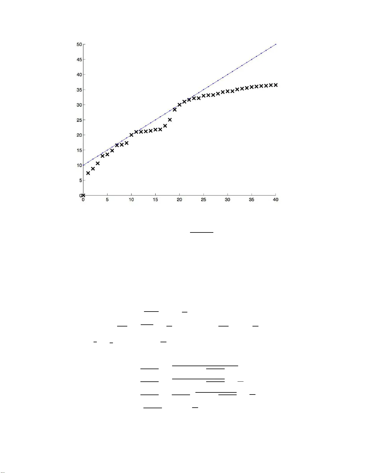
Technical Repor t 73 IMSV, University of Be rn Adaptiv e Confidenc e Sets for the Optimal Appro ximating Mo del Angelik a Rohde Universit¨ at Hambur g Dep artment Mathematik Bundesstr aße 55 D-20146 Hambur g Germany e-mail: ang elika.rohde@ma th.uni-hamburg.de and Lutz D¨ um bgen Universit¨ at Bern Institut f¨ ur Mathematisc he Statistik und V ersicherung slehr e Sid lerstr asse 5 CH-3012 Bern Switzerland e-mail: duembgen @stat.unibe.c h Universit¨ at Hambur g and Universit¨ at Bern Abstract: In the setting of high-dimensional linear models with Gaussian n oise, w e i nv estigate the p ossibilit y of confid ence statements connected to model selectio n. Although there exist n umerous procedures for adaptive (point) estimation, the con- struction of adaptive confidence regions is seve rely limited (cf. Li, 1989). The present pap er shed s new ligh t on this gap. W e deve lop exact and adaptive confidence sets for the b est appro ximating mo del in terms of risk. One of our construct ions is based on a m ultiscale procedure and a particular coupling argumen t. Utilizing exp onential inequalities for noncentral χ 2 -distributions, we sho w th at the risk and quadratic loss of all models within our confidence region are u niformly b ounded by the minimal risk times a f actor clos e to one. AMS 2000 sub ject classifications: 62G15, 62G2 0. Keywords and phrases: Ad aptivity , confidence sets, coupling, ex p onential in eq ual- it y , mo del selectio n, m ultiscale inference, risk optimality .. ∗ This work w as supported b y the Swiss National Science F oun dation. 1 A. R ohde and L. D¨ umb gen/Confidenc e Sets for the Best Appr oximating Mo del 2 1. In tro duction When dealing with a high d imensional observ ation v ector, th e natural qu estion arises whether the data generating pro cess can b e appro ximated b y a mod el of substan tially lo wer dimension. Rather than on the true mo del, the fo cus is here on smaller ones whic h still con tain the essen tial information and allo w for interpretatio n. T ypically , the models u nder consideration are c haracterized b y the non-zero comp onen ts of some parameter v ector. Estimating the true mo del requ ir es the rather id ealistic s ituation th at eac h comp onen t is either equals zero or h as su fficien tly mo d ulus: A tiny p erturb ation of the parameter vect or ma y result in the biggest mod el, so the question ab out the true mo del do es not seem to b e adequate in general. Alternativ ely , th e mo del which is optimal in terms of risk app ears as a target of man y mo del selection strategies. Within a sp ecified class of comp eting mo dels, this pap er is conce rned with confid ence regi ons for those appro ximating mo dels which are optimal in terms of r isk. Supp ose that w e observe a random v ector X n = ( X in ) n i =1 with distribution N n ( θ n , σ 2 I n ) together with an estimator ˆ σ n for the standard deviation σ > 0. O ften the signal θ n represent s co efficien ts of an un kno wn smo oth function with r esp ect to a giv en orthonormal basis of functions. There is a v ast amount of literature on p oin t estimation of θ n . F or a giv en estimator ˆ θ n = ˆ θ n ( X n , ˆ σ n ) for θ n , let L ( ˆ θ n , θ n ) := k ˆ θ n − θ n k 2 and R ( ˆ θ n , θ n ) := E L ( ˆ θ n , θ n ) b e its quadratic loss and the corresp onding risk, resp ectiv ely . Here k· k denotes the standard Euclidean norm of vec tors. V arious adaptivit y results are kno wn for this setting, often in terms of oracle inequalitie s. A t ypical r esult reads as follo ws: Let ( ˇ θ ( c ) n ) c ∈C n b e a family of candidate estimato rs ˇ θ ( c ) n = ˇ θ ( c ) n ( X n ) for θ n , wh ere σ > 0 is temp orarily assumed to b e kno wn. Then there exist estimators ˆ θ n and constant s A n , B n = O (log ( n ) γ ) with γ ≥ 0 suc h that for arbitrary θ n in a certain set Θ n ⊂ R n , R ( ˆ θ n , θ n ) ≤ A n inf c ∈C n R ( ˇ θ ( c ) n , θ n ) + B n σ 2 . Results of this type are provided, for instance, b y Po ly ak and Tsybako v (199 1) and Donoho and Johnstone (1994, 1995, 1998 ), in the framew ork of Gaussian mo del selection by Birg ´ e and Massart (2001). Th e latter article cop es in particular with the fact th at a mo del is A. R ohde and L. D¨ umb gen/Confidenc e Sets for the Best Appr oximating Mo del 3 not n ecessarily true. F ur ther resu lts of this typ e, partly in different settings, hav e b een pro vided by Stone (1984), Lepski et al. (1997), E fromo vic h (1998), Cai (1999, 2002), to men tion just a few. By w a y of contrast, when aiming at adaptiv e confiden ce sets one faces s evere limita- tions. Here is a r esult of L i (1989), sligh tly reph rased: Supp ose that Θ n con tains a closed Euclidean ball B ( θ o n , cn 1 / 4 ) around some v ector θ o n ∈ R n with r ad iu s cn 1 / 4 > 0. Still as- suming σ to b e known, let ˆ D n = ˆ D n ( X n ) ⊂ Θ n b e a (1 − α )-confidence set for θ n ∈ Θ n . Suc h a confidence set ma y b e used as a test of the (Ba yesia n) null hyp othesis that θ n is uniformly distributed on the sphere ∂ B ( θ o n , cn 1 / 4 ) v ersus the alt ernativ e that θ n = θ o n : W e reject this null h yp othesis at lev el α if k η − θ o n k < cn 1 / 4 for all η ∈ ˆ D n . Since this test cannot ha v e larger p o w er than the corresp ond ing Neyman-P earson test, P θ o n  sup η ∈ ˆ D n k η − θ o n k n < cn 1 / 4  ≤ P  S 2 n ≤ χ 2 n ; α ( c 2 n 1 / 2 /σ 2 )  ( S 2 n ∼ χ 2 n ) = Φ  Φ − 1 ( α ) + 2 − 1 / 2 c 2 /σ 2  + o (1 ) , where χ 2 n ; α ( δ 2 ) stands for the α -quant ile of the noncent ral chi-squared distribu tion with n degrees of freedom and n oncen tralit y p arameter δ 2 . Throughou t this pap er, asymptotic statemen ts r efer to n → ∞ . The p r evious inequalit y ent ails th at no reasonable confidence set h as a diameter of o rder o p ( n 1 / 4 ) un iformly o v er the p arameter space Θ n , as long as the latter is sufficien tly large. Despite these limitations, th ere is some literature on confidence sets in the presen t or similar settings; see for instance Beran (1996, 2000), Beran and D ¨ um bgen (1998) and Geno v ese and W assermann (2005). Improvi ng the r ate of O p ( n 1 / 4 ) is only p ossible via additional co nstraints on θ n , i.e. con- sidering substanti ally sm aller sets Θ n . F or instance, Baraud (2004) deve lop ed nonasymp- totic confidence regions whic h p erform w ell on finitely man y linear subspaces. Robins and v an der V aart (2006) construct confid ence balls via samp le splitting whic h adapt to some exten t to the unkno wn “smoothn ess” of θ n . In their co nte xt, Θ n corresp onds to a Sob olev smo othness class with giv en parameter ( β , L ). Ho w ev er, adaptation in this con text is p ossi- ble only within a range [ β , 2 β ]. Indep en den tly , Cai and Lo w (2006) treat the same pr oblem in the sp ecial case of the Gaussian white noise mo del, obtaining the same kind of adap- tivit y in the b roader scale of Beso v b o dies. Other p ossible constrain ts on θ n are so-called shap e constrain ts; see for instance Cai and Low (2007), D ¨ um bgen (2003 ) or Hengartner and Stark (1995) . A. R ohde and L. D¨ umb gen/Confidenc e Sets for the Best Appr oximating Mo del 4 The q u estion is whether one can b ridge this gap b et w een co nfid ence sets and p oin t esti- mators. More precisely , w e wo uld like to understand the p ossibilit y of adaptat ion for p oint estimators in terms of some confidence region for the s et of all optimal candidate estima- tors ˇ θ ( c ) n . That means, w e wan t to construct a confidence region ˆ K n,α = ˆ K n,α ( X n , ˆ σ n ) ⊂ C n for th e set K n ( θ n ) := argmin c ∈C n R ( ˇ θ ( c ) n ) = n c ∈ C n : R ( ˇ θ ( c ) n , θ n ) ≤ R ( ˇ θ ( c ′ ) n , θ n ) for all c ′ ∈ C n o suc h that for arbitrary θ n ∈ R n , P θ n  K n ( θ n ) ⊂ ˆ K n,α  ≥ 1 − α (1) and max c ∈ ˆ K n,α R ( ˇ θ ( c ) n , θ n ) max c ∈ ˆ K n,α L ( ˇ θ ( c ) n , θ n )      = O p ( A n ) min c ∈C n R ( ˇ θ ( c ) n , θ n ) + O p ( B n ) σ 2 . (2) Solving this problem means that stat istical inference ab out differences in the p erformance of estimators is p ossib le, although in ference ab out their risk and loss is sev erely limited. In some settings, select ing estimators out of a class of comp eting estimators en tails esti- mating implicitly an unknown regularit y or smo othness class for the underlying signal θ n . Computing a confidence region for go o d estimat ors is p articularly suitable in situations in whic h sev eral go o d cand id ate estimators fit the data equally w ell although they lo ok differen t. Th is asp ect of exploring v arious candidate est imators is not co v ered b y the usu al theory of p oint estimation. Note that our confid ence region ˆ K n,α is required to con tain the whole set K n ( θ n ), not just one elemen t of it, with probabilit y at least 1 − α . The same requirement is used by F u tsc hik (1999) for inf erence ab out the argmax of a regression f unction. The r emainder of this pap er is organized as follo ws. F or the reader’s con v enience our approac h is fir st d escrib ed in a simple to y mo del in Section 2. In Section 3 w e dev elop a nd analyze an explicit confidence regio n ˆ K n,α related to C n := { 0 , 1 , . . . , n } with candidate estimators ˇ θ ( k ) n :=  1 { i ≤ k } X in  n i =1 . These corresp ond to a standard nested sequence of app ro ximating mo d els. Section 4 d is- cusses r ic her families of candidate estimators. All pro ofs an d auxiliary results are deferr ed to S ections 5 and 6. A. R ohde and L. D¨ umb gen/Confidenc e Sets for the Best Appr oximating Mo del 5 2. A to y problem Supp ose we observe a sto chastic pro cess Y = ( Y ( t )) t ∈ [0 , 1] , where Y ( t ) = F ( t ) + W ( t ) , t ∈ [0 , 1] , with an un kno wn fixed cont inuous function F on [0 , 1] and a Bro wnian m otion W = ( W ( t )) t ∈ [0 , 1] . W e are inte rested in the set S ( F ) := argmin t ∈ [0 , 1] F ( t ) . Precisely , w e wan t to construct a (1 − α )-confidence r egion ˆ S α = ˆ S α ( Y ) ⊂ [0 , 1] for S ( F ) in th e sense that P  S ( F ) ⊂ ˆ S α  ≥ 1 − α, (3) regardless of F . T o construct suc h a confidence set we regard Y ( s ) − Y ( t ) for arbitrary differen t s, t ∈ [0 , 1] as a test statistic f or the n ull h yp othesis that s ∈ S ( F ), i.e. large v alues of Y ( s ) − Y ( t ) giv e evid en ce f or s 6∈ S ( F ). A fir st n aiv e p rop osal is the set ˆ S naiv e α := n s ∈ [0 , 1] : Y ( s ) ≤ min [0 , 1] Y + κ naiv e α o with κ naiv e α denoting the (1 − α )-quan tile of m ax [0 , 1] W − min [0 , 1] W . Here is a refined version based on r esults of D¨ umbgen and Sp oko iny (2001 ): Let κ α b e the (1 − α )-quanti le of sup s,t ∈ [0 , 1]  | W ( s ) − W ( t ) | p | s − t | − q 2 log ( e/ | s − t | )  . (4) Then constrain t (3) is satisfied by the confid en ce region ˆ S α whic h consists of all s ∈ [0 , 1] suc h that Y ( s ) ≤ Y ( t ) + q | s − t |  q 2 log ( e/ | s − t | ) + κ α  for all t ∈ [0 , 1] . T o illustrate the p o w er of this metho d, consider f or in stance a sequence of fun ctions F = F n = c n F o with p ositiv e constants c n → ∞ and a fixed con tin uous function F o with unique minimizer s o . Supp ose that lim t → s o F o ( t ) − F o ( s o ) | t − s o | γ = 1 A. R ohde and L. D¨ umb gen/Confidenc e Sets for the Best Appr oximating Mo del 6 for s ome γ > 1 / 2. Th en the n aiv e confidence region satisfies only max t ∈ ˆ S naive α | t − s o | = O p  c − 1 /γ n  , (5) whereas max t ∈ ˆ S α | t − s o | = O p  log( c n ) 1 / (2 γ − 1) c − 2 / (2 γ − 1) n  . (6) 3. Confidence regions for nested approximating mo dels As in the in tro du ction let X n = θ n + ǫ n denote the n -dimensional observ ation v ecto r with θ n ∈ R n and ǫ n ∼ N n (0 , σ 2 I n ). F or an y cand idate estimator ˇ θ ( k ) n =  1 { i ≤ k } X in  n i =1 the loss is given b y L n ( k ) := L ( ˇ θ ( k ) n , θ n ) = n X i = k +1 θ 2 in + k X i =1 ( X in − θ in ) 2 with corresp ondin g risk R n ( k ) := R ( ˇ θ ( k ) n , θ n ) = n X i = k +1 θ 2 in + kσ 2 . Mo del selection usu ally aims at estimating a candidate estimator whic h is optimal in terms of risk. Since the risk dep ends on the unk n o wn signal and therefore is not a v ailable, the selection pro cedu re minimizes an u nbiased risk estimator instead. In the sequel, th e bias-corrected risk estimator for the candidate ˇ θ ( k ) n is d efined as ˆ R n ( k ) := n X i = k +1 ( X 2 in − ˆ σ 2 n ) + k ˆ σ 2 n , where ˆ σ 2 n is a v ariance estimator satisfying the subsequ en t condition. (A) ˆ σ 2 n and X n are sto c hastically ind ep endent with m ˆ σ 2 n σ 2 ∼ χ 2 m , where 1 ≤ m = m n ≤ ∞ with m = ∞ meaning th at σ is kno wn, i.e. ˆ σ 2 n ≡ σ 2 . F or asymptotic statemen ts, it is generally assumed that β 2 n := 2 n m n = O (1) unless stated otherwise. A. R ohde and L. D¨ umb gen/Confidenc e Sets for the Best Appr oximating Mo del 7 Example. Sup p ose that we observ e Y = M η + δ with giv en design matrix M ∈ R ( n + m ) × n of rank n , un kno wn parameter v ector η ∈ R n and un observ ed error v ector δ ∼ N n + m (0 , σ 2 I n + m ). Then the pr evious assumptions are satisfied b y X n := ( M ⊤ M ) 1 / 2 ˆ η with ˆ η := ( M ⊤ M ) − 1 M ⊤ Y and ˆ σ 2 n := k Y − M ˆ η k 2 /m , where θ n := ( M ⊤ M ) 1 / 2 η . Imp ortant for our analysis is the b eha vior of the cen tered and rescaled difference pr o cess ˆ D n =  ˆ D n ( j, k )  0 ≤ j 2 , ˆ d n := sup 0 ≤ j j  with c j k n = c j k n,α := s 6 | k − j |  Γ  k − j n  + κ n,α  + 3 | k − j | Γ  k − j n  2 . Theorem 3. L et ( θ n ) n ∈ N b e arbitr ary. With ˆ K n,α as define d ab ove, P θ n  K n ( θ n ) 6⊂ ˆ K n,α  ≤ α. In c ase of β n → 0 (i.e. n /m → 0 ), the critic al values κ n,α c onver ge to the critic al value κ α intr o duc e d in Se ction 2. In g ener al, κ n,α = O (1) , and the c onfidenc e r e g i ons ˆ K n,α satisfy the or acle ine qualities max k ∈ ˆ K n,α R n ( k ) ≤ min j ∈C n R n ( j ) +  4 √ 3 + o p (1)  r σ 2 log( n ) min j ∈C n R n ( j ) (10) + O p  σ 2 log n  and max k ∈ ˆ K n,α L n ( k ) ≤ min j ∈C n L n ( j ) + O p  r σ 2 log( n ) min j ∈C n L n ( j )  (11) + O p  σ 2 log n  . Remark (Dep endence on α ) The pr o of rev eals a refined v ersion of the b ounds in Theorem 3 in case of signals θ n suc h that log( n ) 3 = O  min j ∈C n R n ( j )  . Let 0 < α ( n ) → 0 s uc h that κ 6 n,α ( n ) = O  min j ∈C n R n ( j )  . Th en max k ∈ ˆ K n,α R n ( k ) ≤ min j ∈C n R n ( j ) +  4 √ 3 p log n + 2 √ 6 κ n,α + O p (1)  r σ 2 min j ∈C n R n ( j ) uniformly in α ≥ α ( n ). A. R ohde and L. D¨ umb gen/Confidenc e Sets for the Best Appr oximating Mo del 11 Remark (V ariance estimation) Instead of Condition (A), one ma y require more gen- erally th at ˆ σ 2 n and X n are indep enden t with √ n  ˆ σ 2 n σ 2 − 1  → D N (0 , β 2 ) for a giv en β ≥ 0. Th is co v ers, for instance, estimat ors used in connectio n with wa vele ts. There σ is estimated b y the median of some high frequency wa velet coefficien ts divided by the normal quan tile Φ − 1 (3 / 4). Th eorem 1 conti nues to hold, and the coupling extends to this situation, to o, with S 2 in th e pro of b eing distr ibuted as n ˆ σ 2 n . Under th is assumption on the external v ariance estimator, the confid ence region ˆ K n,α , d efined with m := ⌊ 2 n/β 2 ⌋ , is at least asymp totically v alid and satisfies the ab ov e oracle inequalitie s as well. 4. Confidence sets in case of la rger families of candidates The p revious result relies strongly on the assu mption of n ested mo d els. It is p ossible to obtain confid ence sets for the optimal appro ximating mo dels in a more general setting, alb eit the r esulting oracle prop ert y is not as strong as in the nested case. In p articular, w e can no longer rely on a coupling r esult b ut need a different construction. F or the r eader’s con v enience, we f o cus on the case of kn o wn σ , i.e. m = ∞ ; see also the remark at the end of this section. Let C n b e a family of ind ex sets C ⊂ { 1 , 2 , . . . , n } with candidate estimators ˇ θ ( C ) :=  1 { i ∈ C } X in  n i =1 and corresp ond in g risks R n ( C ) := R ( ˇ θ ( C ) , θ n ) = X i 6∈ C θ 2 in + | C | σ 2 , where | S | denotes the cardinalit y of a set S . F or t w o ind ex sets C and D , σ − 2  R n ( D ) − R n ( C )  = δ 2 n ( C \ D ) − δ 2 n ( D \ C ) + | D | − | C | with the auxiliary quantit ies δ 2 n ( J ) := X i ∈ J θ 2 in /σ 2 , J ⊂ { 1 , 2 , . . . , n } . Hence we ai m at sim ultaneous (1 − α )-co nfid en ce inte rv als for these n oncen tralit y param- eters δ n ( J ), where J ∈ M n := { D \ C : C , D ∈ C n } . T o this end w e utilize the fact A. R ohde and L. D¨ umb gen/Confidenc e Sets for the Best Appr oximating Mo del 12 that T n ( J ) := 1 σ 2 X i ∈ J X 2 in has a χ 2 | J | ( δ 2 n ( J ))-distribu tion. W e den ote the distribution function of χ 2 k ( δ 2 ) b y F k ( · | δ 2 ). No w le t M n := |M n | − 1 ≤ |C n | ( |C n | − 1), the num b er of non v oid ind ex sets J ∈ M n . Th en with probabilit y at least 1 − α , α/ (2 M n ) ≤ F | J |  T n ( J )   δ 2 n ( J )  ≤ 1 − α/ (2 M n ) for ∅ 6 = J ∈ M n . (12) Since F | J | ( T n ( J ) | δ 2 ) is str ictly decreasing in δ 2 with limit 0 as δ 2 → ∞ , (12) en tails th e sim ultaneous (1 − α )-confidence interv als  ˆ δ 2 n,α,l ( J ) , ˆ δ 2 n,α,u ( J )  for all parameters δ 2 n ( J ) as follo ws: W e s et ˆ δ 2 n,α,l ( ∅ ) := ˆ δ 2 n,α,u ( ∅ ) := 0, while for nonv oid J , ˆ δ 2 n,α,l ( J ) := m in n δ 2 ≥ 0 : F | J |  T n ( J )   δ 2  ≤ 1 − α/ (2 M n ) o , (13) ˆ δ 2 n,α,u ( J ) := m ax n δ 2 ≥ 0 : F | J |  T n ( J )   δ 2  ≥ α/ (2 M n ) o . (14) By means of these b ound s, w e ma y claim with confid ence 1 − α th at for arbitrary C, D ∈ C n the n ormalized difference ( n/σ 2 )  R n ( D ) − R n ( C )  is at m ost ˆ δ 2 n,α,u ( C \ D ) − ˆ δ 2 n,α,l ( D \ C ) + | D | − | C | . Thus a (1 − α )-co nfid ence set for K n ( θ n ) = argmin C ∈C n R n ( C ) is giv en by ˆ K n,α := n C ∈ C n : ˆ δ 2 n,α,u ( C \ D ) − ˆ δ 2 n,α,l ( D \ C ) + | D | − | C | ≥ 0 f or all D ∈ C n o . These confi dence sets ˆ K n,α satisfy the f ollo wing oracle inequ alities: Theorem 4. L et ( θ n ) n ∈ N b e arbitr ary, and supp ose that log |C n | = o ( n ) . Then max C ∈ ˆ K n,α R n ( C ) ≤ min D ∈C n R n ( D ) + O p  r σ 2 log( |C n | ) min D ∈C n R n ( D )  + O p  σ 2 log |C n |  and max C ∈ ˆ K n,α L n ( C ) ≤ min D ∈C n L n ( D ) + O p  r σ 2 log( |C n | ) min D ∈C n L n ( D )  + O p  σ 2 log |C n |  . Remark. The up p er b ounds in Th eorem 4 are of the form ρ n  1 + O p  q σ 2 log( |C n | ) /ρ n + σ 2 log( |C n | ) /ρ n  with ρ n denoting minimal risk or m inimal loss. Thus Theorem 4 en tails that the m aximal risk (loss) o v er ˆ K n,α exceeds the minimal risk (loss) only by a fact or close to one, pro vided that the minimal risk (loss) is substantia lly larger th an σ 2 log |C n | . A. R ohde and L. D¨ umb gen/Confidenc e Sets for the Best Appr oximating Mo del 13 Remark ( Sub optimality in case of nested mo dels) In case of nested mo d els, the general construction is sub optimal in the factor of the leading (in most cases) term q min j R n ( j ). F ollo wing the pro of carefully and usin g that σ 2 log |C n | = 2 σ 2 log n + O (1) in th is sp ecial setting, one ma y verify that max k ∈ ˆ K n,α R n ( k ) ≤ min j ∈C n R n ( j ) +  4 √ 8 + o p (1)  r σ 2 log( n ) min j ∈C n R n ( j ) + O p  σ 2 log n  . The intrinsic reason is that the general p ro cedur e d o es n ot assume an y structure of the family of candidate estimators. Hence adv anced multi scale theory is not applicable. Remark. In case of un kno wn σ , let α ′ := 1 − (1 − α ) 1 / 2 . Th en with pr ob ab ility at least 1 − α ′ , α ′ / 2 ≤ F m  m ( ˆ σ n /σ ) 2   0  ≤ 1 − α ′ / 2 . The latter inequalities en tail that ( σ/ ˆ σ n ) 2 lies b et w een τ n,α,l := m/χ m ;1 − α ′ / 2 and τ n,α,u := m/χ 2 m ; α ′ / 2 . Th en w e obtain sim u ltaneous (1 − α )-c onfiden ce b ounds ˆ δ 2 n,α,l ( J ) and ˆ δ 2 n,α,u ( J ) as in (13) and (14) by r eplacing α with α ′ and T n ( J ) w ith τ n,α,l ˆ σ 2 n X i ∈ J X 2 in and τ n,α,u ˆ σ 2 n X i ∈ J X 2 in , resp ectiv ely . The conclusions of Th eorem 4 conti nue to hold, as long as n/m n = O (1). 5. Proofs 5.1. Pr o of of (5 ) and (6) Note first that min [0 , 1] Y lies b et w een F n ( s o ) + min [0 , 1] W and F n ( s o ) + W ( s o ). Hence for an y α ′ ∈ (0 , 1), ˆ S naiv e α ⊂  s ∈ [0 , 1] : F n ( s ) + W ( s ) ≤ F n ( s o ) + W ( s o ) + κ naiv e α  ⊂  s ∈ [0 , 1] : F n ( s ) − F n ( s o ) ≤ κ naiv e α ′ + κ naiv e α  =  s ∈ [0 , 1] : F o ( s ) − F o ( s o ) ≤ c − 1 n  κ naiv e α ′ + κ naiv e α  and ˆ S naiv e α ⊃  s ∈ [0 , 1] : F n ( s ) + W ( s ) ≤ F n ( s o ) + min [0 , 1] W + κ naiv e α  ⊃  s ∈ [0 , 1] : F n ( s ) − F n ( s o ) ≤ κ naiv e α − κ naiv e α ′  =  s ∈ [0 , 1] : F o ( s ) − F o ( s o ) ≤ c − 1 n  κ naiv e α − κ naiv e α ′  A. R ohde and L. D¨ umb gen/Confidenc e Sets for the Best Appr oximating Mo del 14 with probabilit y 1 − α ′ . Since κ naiv e α ′ < κ naiv e α if α < α ′ < 1, these considerations, co m bined with the expans ion of F o near s o , sho w that the maximum of | s − s o | ov er all s ∈ ˆ S naiv e α is precisely of order O p ( c − 1 /γ n ). On the other hand, the confidence regio n ˆ S α is con tained in the set of all s ∈ [0 , 1] such that F n ( s ) + W ( s ) ≤ F n ( s o ) + W ( s o ) + q | s − s o |  q 2 log ( e/ | s − s o | ) + κ α o , and this entails th at F o ( s ) − F o ( s o ) ≤ c − 1 n q | s − s o |  q 2 log ( e/ | s − s o | ) + κ α + O p (1)  with O p (1) not d ep end ing on s . No w the expansion of F o near s o en tails claim (6). ✷ 5.2. Exp o nential ine qualities An essen tial ingredient f or our main results is an exp onen tial inequalit y for quadratic functions of a Gaussian random ve ctor. It extends inequalities of Dahlhaus and Polo nik (2006 ) for qu adratic forms and is of ind ep endent in terest. Prop osition 5. L et Z 1 , . . . , Z n b e indep endent, standar d Gaussian r andom variables. F ur- thermor e, let λ 1 , . . . , λ n and δ 1 , . . . , δ n b e r e al c onstants, and define γ 2 := V ar  P n i =1 λ i ( Z i + δ i ) 2  = P n i =1 λ 2 i (2 + 4 δ 2 i ) . Then for arbitr ary η ≥ 0 and λ max := max( λ 1 , . . . , λ n , 0) , P  n X i =1 λ i  ( Z i + δ i ) 2 − (1 + δ 2 i )  ≥ η γ  ≤ exp  − η 2 2 + 4 η λ max /γ  ≤ e 1 / 4 exp  − η / √ 8  . Note that replacing λ i in P rop osition 5 with − λ i yields tw osided exp onential inequali- ties. By means of P r op osition 5 and elemen tary cal culations one obtains exp onen tial and related in equalities for noncen tral χ 2 distributions: Corollary 6. F or an inte g e r n > 0 and a c onstant δ ≥ 0 let F n ( · | δ 2 ) b e the distribution function of χ 2 n ( δ 2 ) . Then for arbitr ary r ≥ 0 , F n ( n + δ 2 + r | δ 2 ) ≥ 1 − exp  − r 2 4 n + 8 δ 2 + 4 r  , (15) F n ( n + δ 2 − r | δ 2 ) ≤ exp  − r 2 4 n + 8 δ 2  . (16) A. R ohde and L. D¨ umb gen/Confidenc e Sets for the Best Appr oximating Mo del 15 In p articular, for any u ∈ (0 , 1 / 2) , F − 1 n (1 − u | δ 2 ) ≤ n + δ 2 + q (4 n + 8 δ 2 ) log( u − 1 ) + 4 log ( u − 1 ) , (17) F − 1 n ( u | δ 2 ) ≥ n + δ 2 − q (4 n + 8 δ 2 ) log( u − 1 ) . (18) Mor e over, for any numb er ˆ δ ≥ 0 , the ine qualities u ≤ F n ( n + ˆ δ 2 | δ 2 ) ≤ 1 − u entail that δ 2 − ˆ δ 2    ≤ + q (4 n + 8 ˆ δ 2 ) log( u − 1 ) + 8 log ( u − 1 ) , ≥ − q (4 n + 8 ˆ δ 2 ) log( u − 1 ) . (19) Conclusion (19) follo ws from (15) and (16), applied to r = ˆ δ 2 − δ 2 and r = δ 2 − ˆ δ 2 , resp ectiv ely . Pro of of Prop osition 5. Standard calculations sh ow that for 0 ≤ t < (2 λ max ) − 1 , E exp  t n X i =1 λ i ( Z i + δ i ) 2  = exp  1 2 n X i =1 n δ 2 i 2 tλ i 1 − 2 tλ i − lo g (1 − 2 tλ i ) o . Then for an y suc h t , P  n X i =1 λ i  ( Z i + δ i ) 2 − (1 + δ 2 i )  ≥ η γ  ≤ exp  − tη γ − t n X i =1 λ i (1 + δ 2 i )  · E exp  t n X i =1 λ i ( Z i + δ i ) 2  = exp  − tη γ + 1 2 n X i =1 n δ 2 i 4 t 2 λ 2 i 1 − 2 tλ i − lo g (1 − 2 tλ i ) − 2 tλ i o . (20 ) Elemen tary considerations r eveal that − log(1 − x ) − x ≤ ( x 2 / 2 if x ≤ 0 , x 2 / (2(1 − x )) if x ≥ 0 . Th us (20) is not greater than exp  − tη γ + 1 2 n X i =1 n δ 2 i 4 t 2 λ 2 i 1 − 2 tλ i + 2 t 2 λ 2 i 1 − 2 t max( λ i , 0) o ≤ exp  − tη γ + γ 2 t 2 / 2 1 − 2 tλ max  . Setting t := η γ + 2 ηλ max ∈ h 0 , (2 λ max ) − 1  , the preceding b oun d b ecomes P  n X i =1 λ i  ( Z i + δ i ) 2 − (1 + δ 2 i )  ≥ η γ  ≤ exp  − η 2 2 + 4 η λ max /γ  . A. R ohde and L. D¨ umb gen/Confidenc e Sets for the Best Appr oximating Mo del 16 Finally , since γ ≥ λ max √ 2, th e second asserted inequ alit y follo ws from η 2 2 + 4 η λ max /γ ≥ η 2 2 + √ 8 η = η √ 8 − η √ 8 + 4 η ≥ η √ 8 − 1 4 . ✷ 5.3. Pr o ofs of the main r esults Throughout this section we assume without loss of generalit y that σ = 1. F ur ther let S n := { 0 , 1 , . . . , n } and T n :=  ( j, k ) : 0 ≤ j < k ≤ n  . Pro of of Theorem 1. Step I . W e first analyze D n in place of ˆ D n . T o collect the necessary ingredient s, let the metric ρ n on T n p oint wise b e defi n ed b y ρ n  ( j, k ) , ( j ′ , k ′ )  := q τ n ( j, j ′ ) 2 + τ n ( k , k ′ ) 2 . W e need b ounds for the capacit y num b ers D( u, T ′ , ρ n ) (cf. Section 6) for certain u > 0 and T ′ ⊂ T . Th e pr o of of Th eorem 2.1 of D ¨ umbgen and S p okoi ny (2001) en tails that D  uδ ,  t ∈ T n : τ n ( t ) ≤ δ  , ρ n  ≤ 12 u − 4 δ − 2 for all u, δ ∈ (0 , 1] . (21) Note that for fixed ( j, k ) ∈ T n , ± D n ( j, k ) ma y b e written as n X i =1 λ i  ( ǫ in + θ in ) 2 − (1 + θ 2 in )  with λ i = λ in ( j, k ) := ±  4 k θ n k 2 + 2 n  − 1 / 2 I ( j,k ] ( i ) , so | λ i | ≤  4 k θ n k 2 + 2 n  − 1 / 2 . Hence it follo ws from Prop osition 5 that P  | D n ( t ) | ≥ τ n ( t ) η  ≤ 2 exp − η 2 2 + 4 η  4 k θ n k 2 + 2 n  1 / 2 /τ n ( t ) ! for arb itrary t ∈ T n and η ≥ 0. On e may rewrite this exp onentia l inequalit y as P  | D n ( t ) | ≥ τ n ( t ) G n  η , τ n ( t )   ≤ 2 exp ( − η ) (22) for arb itrary t ∈ T n and η ≥ 0, wh ere G n  η , δ  := p 2 η + 4 η  4 k θ n k 2 + 2 n  1 / 2 δ . A. R ohde and L. D¨ umb gen/Confidenc e Sets for the Best Appr oximating Mo del 17 The second exp onential inequalit y in Pr op osition 5 entails th at P    D n ( t )   ≥ τ n ( t ) η  ≤ 2 e 1 / 4 exp  − η / √ 8  (23) and P    D n ( s ) − D n ( t )   ≥ √ 8 ρ n ( s, t ) η  ≤ 2 e 1 / 4 exp( − η ) (24) for arb itrary s , t ∈ T n and η ≥ 0. Utilizing (21) and (24), it follo ws fr om Theorem 7 and the subsequent Remark 3 in D ¨ um bgen and W alt her (2007 ) that lim δ ↓ 0 sup n P  sup s,t ∈T n : ρ n ( s,t ) ≤ δ | D n ( s ) − D n ( t ) | ρ n ( s, t ) log  e/ρ n ( s, t )  > Q  = 0 (25) for a su itable constant Q > 0. Since D n ( j, k ) = D n (0 , k ) − D n (0 , j ) and τ n ( j, k ) = ρ n  (0 , j ) , (0 , k )  , this enta ils th e sto c hastic equicont inuit y of D n with resp ect to ρ n . F or 0 ≤ δ < δ ′ ≤ 1 defin e T n ( δ , δ ′ ) := sup t ∈T n : δ <τ n ( t ) ≤ δ ′ | D n ( t ) | τ n ( t ) − Γ n ( t ) − c · Γ n ( t ) 2 τ n ( t )  4 k θ n k 2 + 2 n  1 / 2 ! + with a constan t c > 0 to b e sp ecified later. Recall that Γ n ( t ) :=  2 log  e/τ n ( t ) 2  1 / 2 . Starting from (21), (22) and (25), Theorem 8 of D ¨ um bgen and W alther (2007) and its subsequent remark imply that T n (0 , δ ) → p 0 as n → ∞ and δ ց 0 , (26) pro vided that c > 2. On the other hand, (21), (23) and (25) ent ail that T n ( δ , 1) = O p (1) for any fixed δ > 0 . (27) No w we are ready to pro v e the first assertion ab ou t ˆ D n . Recall that ˆ D n = ˆ σ − 2 n ( D n + V n ) and V n ( j, k ) τ n ( j, k ) = 2 β n ( k − j ) τ n ( j, k )  4 k θ n k 2 + 2 n  1 / 2 √ n Z n with Z n b eing asymptotically standard normal. S in ce τ n ( j, k ) ≤ p 2( k − j ) /  4 k θ n k 2 + 2 n  1 / 2 , | V n ( j, k ) | τ n ( j, k ) ≤ p 2( k − j ) √ n β n | Z n | ≤ γ n ( j, k ) √ n β n | Z n | , (28) so the maximum of | V n | /τ n o v er T n is b oun ded by √ 2 β n | Z n | = O p (1). F urthermore, since |T n | ≤ n 2 / 2, on e can easily deduce from (23) that the maximum of | D n | /τ n o v er T n exceeds A. R ohde and L. D¨ umb gen/Confidenc e Sets for the Best Appr oximating Mo del 18 √ 32 log n + η with probabilit y at most e 1 / 4 exp  − η / √ 8  . Since ˆ σ n = 1 + O p ( n − 1 / 2 ), these considerations sho w that max t ∈T n   ( D n + V n )( t ) | τ n ( t ) ≤ √ 32 log n + O p (1) and max t ∈T n   ˆ D n ( t ) − ( D n + V n )( t )   τ n ( t ) = O p ( n − 1 / 2 log n ) . This prov es our fi rst assertion ab out ˆ D n /τ n . Step I I. Because ˆ σ 2 n → p 1, it is sufficien t for th e pr o of of the weak appr o ximation d w   ˆ D n ( t )  t ∈T n ,  ∆ n ( t )  t ∈T n  → 0 as n → ∞ (29) to show the result for ˆ σ 2 n ˆ D n = D n + V n with the pro cesses D n and V n in tro duced in (7) and (8). Here, d w refers to the dual b ounded Lipsc hitz metric whic h metrizes the top ology of w eak conv ergence. F u r ther details are pro vided in the app endix. Note that D n ( j, k ) = D n ( k ) − D n ( j ) with D n ( ℓ ) := D n (0 , ℓ ) and V n ( j, k ) = V n ( k ) − V n ( j ) with V n ( ℓ ) := V n (0 , ℓ ). Th us w e view these pro cesses D n and V n temp orarily as pro cesses on S n . They are sto c hastically ind ep end ent by Assumption (A). Hence, acccording to Lemma 9, it suffices to s h o w that D n and V n are appro ximated in distribu tion by  W ( τ n ( k ))  k ∈S n and  k √ n p 4 k θ n k 2 + 2 n Z  k ∈S n , (30) resp ectiv ely . The assertion ab out V n is an immediate consequence of the fact that Z n := p m/ 2(1 − ˆ σ 2 n ) = β − 1 n √ n (1 − ˆ σ 2 n ) con ve rges in d istribution to Z while 0 ≤ k /  √ n  4 k θ n k 2 + 2 n  1 / 2  ≤ 1 / √ 2. It remains to v erify the assertion about D n . I t follo ws fr om the results in step I that the sequence of pro cesses D n on S n is sto c hastically equicon tin uous w ith resp ect to th e metric τ n on S n × S n . More pr ecisely , max ( j,k ) ∈T n | D n ( k ) − D n ( j ) | τ n ( j, k ) log ( e/τ n ( j, k ) 2 ) = O p (1) , and it is we ll-kno wn that  W ( τ n (0 , k ) 2 )  k ∈S n has the same prop ert y , ev en with the factor log( e/τ n ( j, k ) 2 ) 1 / 2 in place of log ( e/τ n ( j, k ) 2 ). Moreo ver, b oth pro cesses ha v e indep endent incremen ts. Thus, in view of Theorem 8 in Section 6, it suffices to sho w that max ( j,k ) ∈T n d w  D n ( j, k ) , W ( τ n (0 , k )) − W ( τ n ( j ))  → 0 . (31) A. R ohde and L. D¨ umb gen/Confidenc e Sets for the Best Appr oximating Mo del 19 T o this end we write D n ( j, k ) = D n, 1 ( j, k ) + D n, 2 ( j, k ) + D n, 3 ( j, k ) with D n, 1 ( j, k ) :=  4 k θ n k 2 + 2 n  − 1 / 2 k X i = j +1 1 {| θ in | ≤ δ n } (2 θ in ǫ in + ǫ 2 in − 1) , D n, 2 ( j, k ) :=  4 k θ n k 2 + 2 n  − 1 / 2 k X i = j +1 1 {| θ in | > δ n } 2 θ in ǫ in , D n, 3 ( j, k ) :=  4 k θ n k 2 + 2 n  − 1 / 2 k X i = j +1 1 {| θ in | > δ n } ( ǫ 2 in − 1) and arbitrary n um b ers δ n > 0 su c h that δ n → ∞ b ut δ n /  4 k θ n k 2 + 2 n  1 / 2 → 0. These three rand om v ariables D n,s ( j, k ) are un correlated and h a v e mean zero. The num b er a n :=   { i : | θ in | > δ n }   satisfies the in equalit y k θ n k 2 ≥ a n δ 2 n , whence E  D n, 3 ( j, k ) 2  ≤ 2 a n 2 n + 4 k θ n k 2 ≤ 1 2 δ 2 n → 0 . Moreo v er, D n, 1 ( j, k ) and D n, 2 ( j, k ) are sto c hastically indep en d en t, where D n, 1 ( j, k ) is asymptotically Gaussian by v ir tue of Lindeb erg’s CL T , while D n, 2 ( j, k ) is exactly Gaus- sian. These findin gs en tail (29). Step I I I. F or 0 ≤ δ < δ ′ ≤ 1 defin e S n ( δ , δ ′ ) := sup t ∈T n : δ<τ n ( t ) ≤ δ ′   ( D n + V n )( t )   τ n ( t ) − Γ n ( t ) − c · Γ n ( t ) 2  4 k θ n k 2 + 2 n  1 / 2 τ n ( t ) ! + , Σ n ( δ , δ ′ ) := sup ( j,k ) ∈T n : δ<τ n ( j,k ) ≤ δ ′    W ( τ n (0 , k ) 2 ) − W ( τ n (0 , j ) 2 )   τ n ( j, k ) − Γ n ( j, k )  + . Since S n (0 , 1) ≤ T n (0 , 1) + √ 2 β n | Z n | , it follo ws fr om (26) and (27) that S n (0 , 1) = O p (1). As to the app ro ximation in distribution, since τ n (0 , n )  4 k θ n k 2 + 2 n  1 / 2 ≥ √ 2 n → ∞ , max t : τ n ( t ) ≥ δ     Γ n ( t ) 2  4 k θ n k 2 + 2 n  1 / 2 τ n ( t )     → 0 w hile max t : τ n ( t ) ≥ δ | Γ n ( t ) | = O (1) for any fi xed δ ∈ (0 , 1). Consequently it follo ws fr om step II that d w  S n ( δ , 1) , Σ n ( δ , 1)  → 0 (32) for any fi xed δ ∈ (0 , 1). Thus it suffi ces to show that S n (0 , δ ) , Σ n (0 , δ ) → p 0 as n → ∞ and δ ց 0 , A. R ohde and L. D¨ umb gen/Confidenc e Sets for the Best Appr oximating Mo del 20 pro vided that k θ n k 2 = O ( n ). F or Σ n (0 , δ ) this claim follo ws, for instance, with the same argumen ts as (26). Moreo v er, S n (0 , δ ) is not greater than T n (0 , δ ) + sup t ∈T n : τ n ( t ) ≤ δ | V n ( t ) | τ n ( t ) ≤ T n (0 , δ ) +  4 k θ n k 2 + 2 n  1 / 2 √ n δ , according to (28). Thus our claim follo ws from (26) and k θ n k 2 = O ( n ). ✷ Pro of of Prop osition 2. The main in gredien t is a well- known represent ation of non- cen tral χ 2 distributions as P oisson mixtures of cen tral χ 2 distributions. Precisely , χ 2 k ( δ 2 ) = ∞ X j =0 e − δ 2 / 2 ( δ 2 / 2) j j ! · χ 2 k +2 j , as can b e pro v ed via Laplace trans forms. No w we defin e ‘time p oin ts’ t k n := k X i =1 θ 2 in and t ∗ k n := t j ( n ) n + k − j ( n ) with j ( n ) any fixed index in K n ( θ n ). This co nstru ction en tails that t ∗ k n ≥ t k n with equ alit y if, and only if, k ∈ K n ( θ n ). Figure 1 illustrates th is construction. It s h o ws the time p oints t k n (crosses) and t ∗ k n (dots and line) versus k for a h yp othetical s ignal θ n ∈ R 40 . Note that in this example, K n ( θ n ) is giv en by { 10 , 11 , 20 , 21 } . Let Π, G 1 , G 2 , . . . , G n , Z 1 , Z 2 , Z 3 , . . . and S 2 b e sto chastic ally in d ep end en t random v ariables, where Π = (Π( t )) t ≥ 0 is a standard Po isson pr o cess, G i and Z j are standard Gaussian random v ariables, and S 2 ∼ χ 2 m . Then on e can easily ve rify that ˜ T j k n := m ( k − j ) S 2  k X i = j +1 G 2 i + 2Π( t kn / 2) X s =2Π( t j n / 2)+1 Z 2 s  , ˜ T ∗ j k n := m ( k − j ) S 2  k X i = j +1 G 2 i + 2Π( t ∗ kn / 2) X s =2Π( t ∗ j n / 2)+1 Z 2 s  define random v ariables ( ˜ T j k n ) 0 ≤ j k , an d γ ( ∗ ) n ( k , k ) := 0. In the subs equ en t arguments, k n := min( K n ( θ n )), w hile j stands for a generic in dex in ˆ K n,α . The definition of the set ˆ K n,α en tails that ˆ R n ( j, k n ) ≤ ˆ σ 2 n h γ ∗ n ( j, k n )  Γ  j − k n n  + κ n,α  + O (log n ) i . (33) Here and sub sequent ly , O ( r n ) and O p ( r n ) denote a generic n um b er and random v ariable, resp ectiv ely , dep ending on n b ut neither on an y other indices in C n nor on α ∈ (0 , 1). Precisely , in view of our remark on depen dence of α , w e consider all α ≥ α ( n ) w ith α ( n ) > 0 suc h that κ n,α ( n ) = O ( n 1 / 6 ). Note that ˆ σ 2 n = 1 + O p ( n − 1 / 2 ). Moreo v er, γ ∗ n ( j, k n ) 2 Γ  ( j − k n ) /n  2 equals 12 nx log ( e/x ) ≤ 12 n with x := | j − k n | /n ∈ [0 , 1]. Thus w e ma y r ewrite (33) as ˆ R n ( j, k n ) ≤ γ ∗ n ( j, k n )  Γ  j − k n n  + κ n,α  + O p (log n ) . (34) Com bining this with the equation R n ( j, k n ) = ˆ R n ( j, k n ) − ˆ D n ( j, k n ) yields R n ( j, k n ) ≤ γ ∗ n ( j, k n )  Γ  j − k n n  + κ n,α  + O p (log n ) + | ˆ D n ( j, k n ) | . (35) Since γ ∗ n ( j, k n ) 2 ≤ 6 n and max t ∈T n | ˆ D n ( t ) | /γ n ( t ) = O p (log n ), (35) yields R n ( j, k n ) ≤ √ 12 n + √ 6 n κ n,α + O p (log n ) γ n ( j, k n ) . But elemen tary calculations yield γ n ( j, k n ) 2 = γ ∗ n ( j, k n ) 2 + sign( k n − j ) R n ( j, k n ) ≤ 6 n + R n ( j, k n ) . (36) Hence we may conclude that R n ( j, k n ) ≤ O p (log n ) q R n ( j, k n ) + O p  √ n (log n + κ n,α )  , A. R ohde and L. D¨ umb gen/Confidenc e Sets for the Best Appr oximating Mo del 23 and Lemma 7 (i), applied to x = 0 and y = R n ( j, k n ), yields max j ∈ ˆ K n,α R n ( j, k n ) ≤ O p  √ n (log n + κ n,α )  . (37) This preliminary result allo ws us to restrict our atten tion to indices j in a certain su b set of C n : Sin ce 0 ≤ R n ( n, k n ) = n − k n − P n i = k n +1 θ 2 in , n X i = k n +1 θ 2 in ≤ n − k n . On the other hand, in case of j < k n , R n ( j, k n ) = P k n i = j +1 θ 2 in − ( k n − j ), so n X i = j +1 θ 2 in ≤ n + O p  √ n (log n + κ n,α )  . Th us if j n denotes the smallest index j ∈ C n suc h that P n i = j +1 θ 2 in ≤ 2 n , then k n ≥ j n , and ˆ K n,α ⊂ { j n , . . . , n } with asymptotic probabilit y one, un iformly in α ≥ α ( n ). This allo ws us to restrict our atten tion to in dices j in { j n , . . . , n } ∩ ˆ K n,α . F or an y ℓ ≥ j n , ˆ D n ( ℓ, k n ) in v olv es only the restricted signal v ector ( θ in ) n i = j n +1 , and the pr o of of T heorem 1 entai ls that max j n ≤ ℓ ≤ n  | ˆ D n ( ℓ, k n ) | γ n ( ℓ, k n ) − p 2 log n − 2 c log n γ n ( ℓ, k n )  + = O p (1) . Th us w e may deduce from (35) the simpler statemen t that w ith asymptotic probabilit y one, R n ( j, k n ) ≤  γ ∗ n ( j, k n ) + γ n ( j, k n )  p 2 log n + κ n,α + O p (1)  (38) + O p (log n ) . No w w e need reasonable b ounds for γ ∗ n ( j, k n ) 2 in terms of R n ( j ) and the min imal risk ρ n = R n ( k n ), w here we start from the equation in (36): If j < k n , then γ n ( j, k n ) 2 = γ ∗ n ( j, k n ) 2 + 4 R n ( j, k n ) and γ ∗ n ( j, k n ) 2 = 6( k n − j ) ≤ 6 ρ n . If j > k n , then γ ∗ n ( j, k n ) 2 = γ n ( j, k n ) 2 + 4 R n ( j, k n ) and γ n ( j, k n ) 2 = j X i = k n +1 (4 θ 2 in + 2) ≤ 4 ρ n + 2 R n ( j ) = 6 ρ n + 2 R n ( j, k n ) . Th us γ ∗ n ( j, k n ) + γ n ( j, k n ) ≤ 2 √ 6 √ ρ n +  √ 2 + √ 6  q R n ( j, k n ) , A. R ohde and L. D¨ umb gen/Confidenc e Sets for the Best Appr oximating Mo del 24 and inequalit y (38) leads to R n ( j, k n ) ≤  4 √ 3 p log n + 2 √ 6 κ n,α + O p (1)  √ ρ n + O p  p log n + κ n,α  q R n ( j, k n ) + O p (log n ) for all j ∈ ˆ K n,α . Again we ma y emp lo y Lemma 7 with x = 0 and y = R n ( j, k n ) to conclud e that max j ∈ ˆ K n,α R n ( j, k n ) ≤  4 √ 3 p log n + 2 √ 6 κ n,α + O p (1)  √ ρ n + O p  (log( n ) 3 / 4 + κ 3 / 2 n,α ( n ) ) ρ 1 / 4 n + lo g n + κ 2 n,α ( n )  uniformly in α ≥ 0. If log( n ) 3 + κ 6 n,α ( n ) = O ( ρ n ), then the p revious b ound for R n ( j, k n ) = R n ( j ) − ρ n reads max j ∈ ˆ K n,α R n ( j ) ≤ ρ n +  4 √ 3 p log n + 2 √ 6 κ n,α + O p (1)  √ ρ n uniformly in α ≥ α ( n ). On the other hand , if we consider just a fixed α > 0, then κ n,α = O (1), and the pr evious considerations yield max j ∈ ˆ K n,α R n ( j ) ≤ ρ n +  4 √ 3 + o p (1)  q log( n ) ρ n + O p  log( n ) 3 / 4 ρ 1 / 4 n + lo g n  ≤ ρ n +  4 √ 3 + o p (1)  q log( n ) ρ n + O p (log n ) . T o v erify the latter step, n ote th at f or any fi x ed ǫ > 0, log( n ) 3 / 4 ρ 1 / 4 n ≤ ( ǫ − 1 log n if ρ n ≤ ǫ − 4 log n, ǫ p log( n ) ρ n if ρ n ≥ ǫ − 4 log n. It remains to pro v e claim (11) ab out the losses. F rom now on, j denotes a ge neric index in C n . Note fi rst that L n ( j, k n ) − R n ( j, k n ) = k n X i = j +1 (1 − ǫ 2 in ) = R n ( k n , j ) − L n ( k n , j ) if j < k . Th us Theorem 1, applied to θ n = 0, shows that   L n ( j, k n ) − R n ( j, k n )   ≤ γ + n ( j, k n )  p 2 log n + O p (1)  + O p (log n ) , where γ + n ( j, k n ) := q 2 | k n − j | ≤ p 2 ρ n + q 2 | R n ( j, k ) | . A. R ohde and L. D¨ umb gen/Confidenc e Sets for the Best Appr oximating Mo del 25 It follo ws from L n (0) = R n (0) = k θ n k 2 that L n ( j ) − ρ n equals L n ( j, k n ) + ( L n − R n )( k n , 0) = R n ( j, k n ) + O p  q log( n ) ρ n  + O p  p log n  q R n ( j, k n ) + O p (log n ) ≥ O p  q log( n ) ρ n + log n  , b ecause R n ( j, k n ) ≥ 0 and R n ( j, k n ) + O p ( r n ) p R n ( j, k n ) ≥ O p ( r 2 n ). Consequen tly , ˆ ρ n := min j ∈C n L n ( j ) satisfies the inequalit y ˆ ρ n ≥ ρ n + O p  q log( n ) ρ n + lo g n  = (1 + o p (1)) ρ n + O p (log n ) , and this is easily shown to en tail that ρ n ≤ ˆ ρ n + O p  p log n  p ˆ ρ n + O p (log n ) = (1 + o p (1)) ˆ ρ n + O p (log n ) . No w we restrict our atten tion to ind ices j ∈ ˆ K n,α again. Here it follo ws from our r esult ab out the maximal risk o v er ˆ K n,α that L n ( j ) − ρ n equals R n ( j, k n ) + O p  q log( n ) ρ n  + O p  p log n  q R n ( j, k n ) + O p (log n ) ≤ 2 R n ( j, k n ) + O p  q log( n ) ρ n + lo g n  ≤ O p  q log( n ) ρ n + lo g n  . Hence m ax j ∈ ˆ K n,α L n ( j ) is not greater than ρ n + O p  q log( n ) ρ n + lo g n  ≤ ˆ ρ n + O p  p log n  p ˆ ρ n + O p (log n ) . ✷ Pro of of Theorem 4. The app lication of inequalit y (19) in Corolla ry 6 to the trip el ( | J | , T n ( J ) − | J | , α/ (2 M n )) in place of ( n, ˆ δ 2 , α ) yields b ounds for ˆ δ 2 n,α,l ( J ) and ˆ δ 2 n,α,u ( J ) in terms of ˆ δ 2 n ( J ) := ( T n ( J ) − | J | ) + . Then we apply (17 -18) to T n ( J ), replacing ( n, δ 2 , u ) with ( | J | , δ 2 n ( J ) , α ′ / (2 M n )) for an y fix ed α ′ ∈ (0 , 1). By m eans of Lemm a 7 (ii) we obtain finally ˆ δ 2 n,α,u ( J ) − δ 2 n ( J ) δ 2 n ( J ) − ˆ δ 2 n,α,l ( J ) ) ≤ (1 + o p (1)) q (16 | J | + 32 δ 2 n ( J )) log M n (39) + ( K + o p (1)) log M n for all J ∈ M n . Here and throughout this pr o of, K denotes a generic constan t not dep end- ing on n . I ts v alue may b e d ifferen t in different expressions. It follo ws from the d efi nition A. R ohde and L. D¨ umb gen/Confidenc e Sets for the Best Appr oximating Mo del 26 of the confi d ence region ˆ K n,α that for arb itrary C ∈ ˆ K n,α and D ∈ C n , R n ( C ) − R n ( D ) = δ 2 n ( D \ C ) − δ 2 n ( C \ D ) + | C | − | D | = ( δ 2 n − ˆ δ 2 n,α,l )( D \ C ) + ( ˆ δ 2 n,α,u − δ 2 n )( C \ D ) −  ˆ δ 2 n,α,u ( C \ D ) − ˆ δ 2 n,α,l ( D \ C ) + | D | − | C |  ≤ ( δ 2 n − ˆ δ 2 n,α,l )( D \ C ) + ( ˆ δ 2 n,α,u − δ 2 n )( C \ D ) . Moreo v er, according to (39) the latter b ound is not larger th an (1 + o p (1)) n q  16 | D \ C | + 32 δ 2 n ( D \ C )  log M n + q  16 | C \ D | + 3 2 δ 2 n ( C \ D )  log M n o + ( K + o p (1)) log M n ≤ (1 + o p (1)) q 2  16 | D | + 32 δ 2 n ( C c ) + 16 | C | + 32 δ 2 n ( D c )  log M n + ( K + o p (1)) log M n ≤ 8 q  R n ( C ) + R n ( D )  log M n (1 + o p (1)) + ( K + o p (1)) log M n . Th us we obtain the quadratic inequalit y R n ( C ) − R n ( D ) ≤ 8 q  R n ( C ) + R n ( D )  log M n (1 + o p (1)) + ( K + o p (1)) log M n , and with Lemma 7 this leads to R n ( C ) ≤ R n ( D ) + 8 √ 2 q R n ( D ) log M n (1 + o p (1)) + ( K + o p (1)) log M n . This yields the assertion ab out the risks . As for the losses, n ote that L n ( · ) and R n ( · ) are closely relate d in that ( L n − R n )( D ) = X i ∈ D ǫ 2 in − | J | for arbitrary D ∈ C n . Hence we may u tilize (17-18), replacing the trip el ( n, δ 2 , u ) with ( | D | , 0 , α ′ / (2 µ n )), to complement (39) w ith th e follo wing observ ation: − A q | D | log M n ≤ L n ( D ) − R n ( D ) ≤ A q | D | log M n + A log M n (40) sim ultaneously f or all D ∈ C n with probabilit y tendin g to one as n → ∞ and A → ∞ . Note also th at (40) implies that R n ( D ) ≤ A p R n ( D ) log M n + L n ( D ). Hence R n ( D ) ≤ (3 / 2)  L n ( D ) + A 2 log M n  for all D ∈ C n , A. R ohde and L. D¨ umb gen/Confidenc e Sets for the Best Appr oximating Mo del 27 b y Lemm a 7 (i). Ass u ming that b oth (39) and (40 ) hold f or some large bu t fixed A , w e ma y conclude that for arbitrary C ∈ ˆ K n,α and D ∈ C n , L n ( C ) − L n ( D ) = ( L n − R n )( C ) − ( L n − R n )( D ) + R n ( C ) − R n ( D ) ≤ A q 2( | C | + | D | ) log M n + A q 2  R n ( C ) + R n ( D )  log M n + 4 A log M n ≤ 2 A q 2  R n ( C ) + R n ( D )  log M n + 4 A log M n ≤ A ′ q  L n ( C ) + L n ( D )  log M n + A ′′ log M n for constants A ′ and A ′′ dep end ing on A . Again this inequalit y enta ils th at L n ( C ) ≤ L n ( D ) + A ′ q 2 L n ( D ) log M n + A ′′′ log M n for another constan t A ′′′ = A ′′′ ( A ). ✷ 6. Auxiliary results This section collec ts some results from th e vicinit y of empirical pro cess theory whic h are used in the p resen t pap er. F or an y p seudo-metric sp ace ( X , d ) and u > 0, we d efi ne th e capacit y n um b er D( u, X , d ) := max  |X o | : X o ⊂ X , d ( x, y ) > u for differen t x, y ∈ X o  . It is w ell-kno wn that conv ergence in distribu tion of random v ariables with v alues in a separable metric sp ace ma y b e metrized by the dual b ounded Lipsc hitz d istance. No w w e adapt th e latter distance for sto c hastic p ro cesses. Let ℓ ∞ ( T ) b e the space of b ounded functions x : T → R , equip p ed with supremum norm k · k ∞ . F o r t w o sto c hastic pro cesses X and Y on T with b oun ded sample paths we defin e d w ( X, Y ) := sup f ∈H ( T )   E ∗ f ( X ) − E ∗ f ( Y )   , where P ∗ and E ∗ denote outer p r obabilities an d exp ectations, r esp ectiv ely , while H ( T ) is the family of all f unt ionals f : ℓ ∞ ( T ) → R suc h that | f ( x ) | ≤ 1 and | f ( x ) − f ( y ) | ≤ k x − y k ∞ for all x, y ∈ ℓ ∞ ( T ) . If d is a pseud o-metric on T , then the mod u lus of contin u it y w ( x, δ | d ) of a fu nction x ∈ l ∞ ( T ) is defin ed as w ( x, δ | d ) := sup s,t ∈T : d ( s,t ) ≤ δ | x ( s ) − x ( t ) | . A. R ohde and L. D¨ umb gen/Confidenc e Sets for the Best Appr oximating Mo del 28 F u rthermore, C u ( T , d ) denotes the set of uniformly con tin uous fun ctions on ( T , d ), that is C u ( T , d ) = n x ∈ l ∞ ( T ) : lim δ ց 0 w ( x, δ | d ) = 0 o . Theorem 8. F or n = 1 , 2 , 3 , . . . c onsider sto chastic pr o c esses X n =  X n ( t )  t ∈T n and Y n =  Y n ( t )  t ∈T n on a metric sp ac e ( T n , ρ n ) with b ounde d sample p aths. Then d w ( X n , Y n ) → 0 pr ovide d that the fol lowing thr e e c onditions ar e satisfie d: (i) F or arbitr ary subsets T n,o of T n with |T n,o | = O (1) , d w  X n   T n,o , Y n   T n,o  − → 0; (ii) for e ach numb er ǫ > 0 , lim δ ց 0 lim sup n →∞ P ∗  w ( Z n , δ | ρ n ) > ǫ  = 0 for Z n = X n , Y n ; (iii) for any δ > 0 , D ( δ, T n , ρ n ) = O (1) . Pro of. F or an y fixed num b er δ > 0 let T n,o b e a maximal subset of T n suc h that ρ n ( s, t ) > δ for differnt s, t ∈ T n,o . Th en |T n,o | = O (1) by Assumption (iii). Moreo v er, f or any t ∈ T n there exists a t o ∈ T n,o suc h that ρ n ( t, t o ) ≤ δ . Hence there exists a partition of T n in to sets B n ( t o ), t o ∈ T n,o , satisfying t o ∈ B n ( t o ) ⊂  t ∈ T n : ρ n ( t, t o ) ≤ δ  . F o r an y function x in ℓ ∞ ( T n ) or ℓ ∞ ( T n,o ) let π n x ∈ ℓ ∞ ( T n ) b e giv en by π n x ( t ) := X t o ∈T n,o 1 { t ∈ B n ( t o ) } x ( t o ) . Then π n x is linear in x   T n,o with k π n x k ∞ =   x   T n,o   ∞ . Moreo v er, any x ∈ ℓ ∞ ( T n ) satisfies the inequalit y k x − π n x k ∞ ≤ w ( x, δ | ρ n ). Hence f or Z n = X n , Y n , d w ( Z n , π n Z n ) ≤ sup h ∈H ( T n ) E ∗   h ( Z n ) − h ( π n Z n )   ≤ E ∗ min  k Z n − π n Z n k ∞ , 1  ≤ E ∗ min  w ( Z n , δ | ρ n ) , 1  , and this is arbitrarily small for s ufficien tly small δ > 0 and s ufficien tly large n , according to Ass u mption (ii). A. R ohde and L. D¨ umb gen/Confidenc e Sets for the Best Appr oximating Mo del 29 F u rthermore, elemen tary considerations revea l th at d w ( π n X n , π n Y n ) = d w  X n   T n,o , Y n   T n,o  , and the latter distance con v erges to zero, b ecause of |T n,o | = O (1) and Assu m ption (i). Since d w ( X n , Y n ) ≤ d w ( X n , π n X n ) + d w ( Y n , π n Y n ) + d w ( π n X n , π n Y n ) , these considerations en tail the assertion that d w ( X n , Y n ) → 0. ✷ Finally , the next lemma p ro vides a useful inequ alit y for d w ( · , · ) in connection with sums of indep endent processes. Lemma 9. L et X = X 1 + X 2 and Y = Y 1 + Y 2 with indep endent r andom varia bles X 1 , X 2 and indep endent r andom variables Y 1 , Y 2 , al l taking values in ( ℓ ∞ ( T ) , k · k ∞ ) . Then d w ( X, Y ) ≤ d w ( X 1 , Y 1 ) + d w ( X 2 , Y 2 ) . F or this lemma it is imp ortan t that we consider random v ariables rather th an just sto c hastic p ro cesses with b oun d ed s ample paths. Note that a sto c hastic pr o cess on T is automatically a random v ariable with v alues in ( ℓ ∞ ( T ) , k · k ∞ ) if (a) the index set T is finite, or (b) th e pro cess has un iformly con tin uous sample paths with resp ect to a pseudo-metric d on T suc h that N ( u, T , d ) < ∞ for all u > 0. Pro of of Lemma 9. Without loss of generalit y let the four random v ariables X 1 , X 2 , Y 1 and Y 2 b e defined on a common p robabilit y space and sto c hastically indep endent. Let f b e an arbitrary fun ctional in H ( T ). Th en it f ollo ws f rom F ubini’s theorem that   E f ( X 1 + X 2 ) − E f ( Y 1 + Y 2 )   ≤   E f ( X 1 + X 2 ) − E f ( Y 1 + X 2 )   +   E f ( Y 1 + X 2 ) − E f ( Y 1 + Y 2 )   ≤ E    E ( f ( X 1 + X 2 ) | X 2 ) − E ( f ( Y 1 + X 2 ) | X 2 )    + E    E ( f ( Y 1 + X 2 ) | Y 1 ) − E ( f ( Y 1 + Y 2 ) | Y 1 )    ≤ d w ( X 1 , Y 1 ) + d w ( X 2 , Y 2 ) . The latter inequalit y follo ws from the fact th at the f unctionals x 7→ f ( x + X 2 ) and x 7→ f ( Y 1 + x ) b elong to H ( T ), to o. Thus d w ( X, Y ) ≤ d w ( X 1 , Y 1 ) + d w ( X 2 , Y 2 ). ✷ Ac kno wledgemen t. Constr u ctiv e comments of a r eferee are gratefully ac knowledged. A. R ohde and L. D¨ umb gen/Confidenc e Sets for the Best Appr oximating Mo del 30 References [1] Baraud, Y. (2004). Confidence balls in Gaussian r egression. Ann. Statist. 32 , 528-5 51. [2] Beran, R. (1996). Confidence sets centered at C p estimators. An n. Ins t. Statist. Math. 48 , 1-15. [3] Beran, R. (2000). REA CT scatterplot smo others: sup erefficiency through basis econom y . J. Amer. Statist. Asso c. 95 , 155-169. [4] Beran, R. and D ¨ umbgen, L. (1998) . Mo d ulation o f estimators and confidence sets. Ann. Statist. 26 , 1826-18 56. [5] Bir g ´ e, L. and Mas sar t, P. (2001). Gaussian mo del selection. J. Eur. Math. So c. 3 , 203-26 8. [6] Cai, T.T. ( 1999). Ad aptiv e wa vel et estimation: a blo ck thresholding and oracle inequalit y appr oac h. Ann. S tatist. 26 , 1783-1 799. [7] Cai, T.T. (2002). On blo c k thresholding in w a velet regression: adaptivit y , block size, and threshold lev el. S tatistica S inica 12 , 1241-1273. [8] Cai, T.T . and Low, M.G. (2006). Adaptiv e confiden ce balls. An n. Statist. 34 , 202-2 28. [9] Cai, T.T. and Low, M.G. (2007). Adaptive estima tion an d confiden ce in terv als for con v ex fun ctions and monotone fu nctions. Man uscript in pr eparation. [10] D ahlhaus, R. and Polonik, W . (2006). Nonparametric quasi-maxim um lik eliho o d estimation for Gaussian lo cally stationary pr o cesses. Ann. Statist. 34 , 2790-28 24. [11] Donoho, D.L. and Joh nstone, I.M . (1994). Id eal spatial adap tation by wa v elet shrink age. Biometrik a 81 , 425-455 . [12] Donoho, D.L. and Johns tone, I.M. (1995). Adapting to unkno wn smo othness via w a v elet shr ink age. J ASA 90 , 1200-1224. [13] Donoho, D.L. and Johnst one, I.M. (1998). Minimax estimation via w a v elet shrink age. Ann. Statist. 26 , 879-921. [14] D ¨ umbgen, L. (200 2). App lication o f local rank tests to nonparametric regression. J . Nonpar. S tatist. 14 , 511-53 7. [15] D ¨ umbgen, L. (2 003). Optimal confid ence b ands for sh ap e-restricted curv es. Bernoulli 9 , 423-44 9. [16] D ¨ umbgen, L. and S pokoiny, V.G . (200 1). Multiscale testing of qualitati ve hy- p otheses. Ann. Statist. 29 , 124-152. [17] D ¨ umbgen, L. and W al t her, G. (2007). Multiscale inference ab ou t a densit y . T ec h- nical r ep ort 56, IMSV, Unive rsit y of Bern. [18] Efromo vich, S. (1998 ). Simultaneo us sharp estimation of fun ctions and their d eriv a- tiv es. Ann . S tatist. 26 , 273-278. [19] Futsch ik, A. (1999). Confid ence r egions for the s et of global maximizers of non- parametrically estimated curves. J. S tatist. Plann. Inf. 82 , 237-250. [20] Genovese, C.R. an d W assermann , L. (2005). Confid ence sets for nonparametric w a v elet regression. Ann. S tatist. 33 , 698-72 9. [21] Hengar tn er, N.W. and St ark , P.B. (1995). Finite-sample confidence en v elop es for s h ap e-restricted densities. Ann. S tatist. 23 , 525-550. [22] Hoffman n, M. and Lepski, O. (200 2). Random rates in anisotropic regression (with discussion). Ann . S tatist. 30 , 325-396. A. R ohde and L. D¨ umb gen/Confidenc e Sets for the Best Appr oximating Mo del 31 [23] Lepski, O.V . , M ammen, E. and S pokoiny, V.G. (1997). Optimal spatial adap- tation to inhomogeneous smo othness: an approac h b ased on k ernel estimates w ith v ariable band width s electors. Ann. Statist. 25 , 929-947. [24] Li, K.-C. ( 1989). Honest confidence regions for n onparametric r egression. Ann. Statist. 17 , 1001-1 008. [25] Pol y ak, B.T. and Tsybako v, A.B. (1991). Asymptotic optimali t y of the C p -test for the orthogonal series estimation of regression. Theory Probab. App l. 35 , 293- 306. [26] R obins, J. and v an der V aar t, A. (200 6). Adaptiv e nonparametric confidence sets. Ann. Statist. 34 , 229-253. [27] Stone, C.J. (1 984). An asymptotically optimal window selection rule for kernel densit y estimates. An n. Statist. 12 , 1285 -1297.