Quantization Errors of fGn and fBm Signals

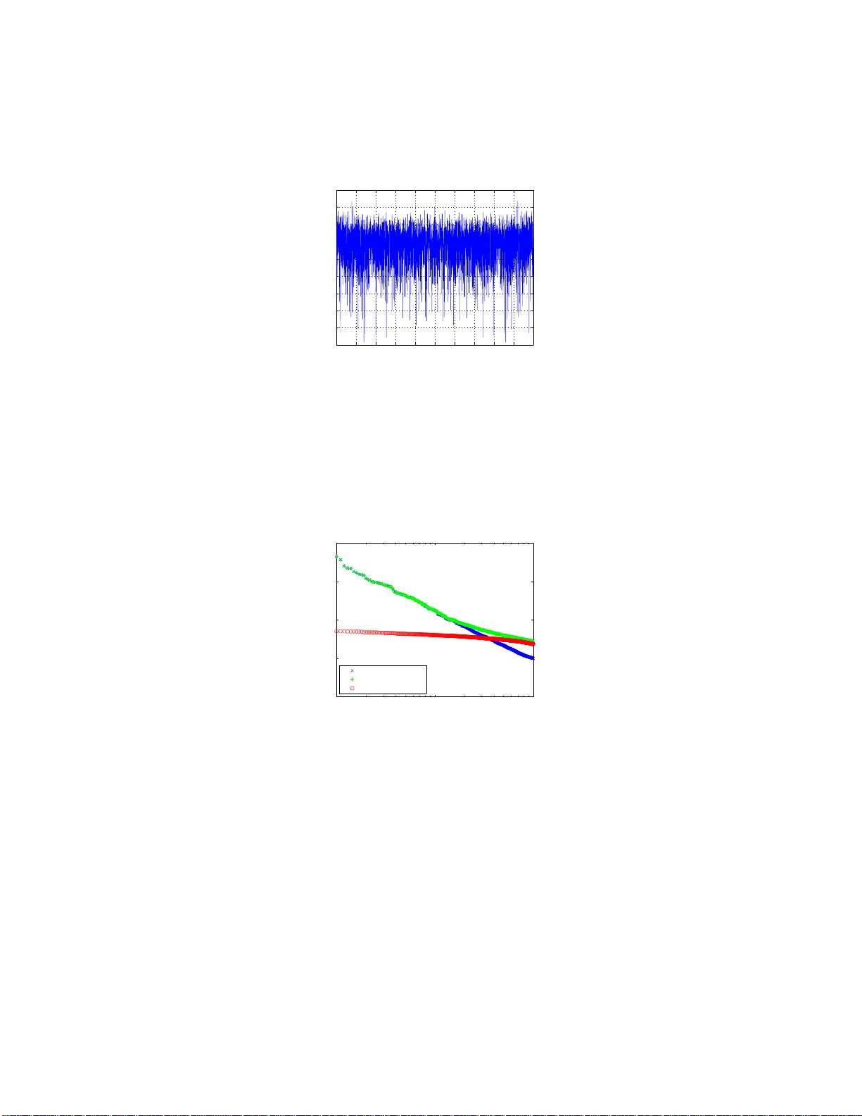
Quan tization Errors of fGn and fBm Signals Zhiheng Li, Li Li ∗ , Y udong Chen, Yi Zhang Departmen t of Automation, Tsingh ua Univ ersit y , Beijing, China 10008 4 No ve mber 3, 2018 Abstract In this Letter, w e show that under th e assumption of high resolution, the quantization errors of fGn and fBm signals with uniform quantizer can b e treated as uncorrelated white noises. 1 In tro d uction F r actional Gaussia n no ise (fGn) a nd fractional Br ownian motion (fBm) provide conv enient wa ys to describ e s to chastic pro c e sses with long-r a nge dep endencie s . Thu s, they ha ve receiv ed contin uing in teres ts in v arious fields and ha ve m a ny applications, e.g . mo deling the communication netw or ks flow a nd economic times ser ies [1]-[3]. Of particula r in ter est is the estimatio n o f the Hurst ex po nent H of a fGn or fBm pr o cess. In pr actice, such estimations ar e usua lly done on the s a mpled and quantized time series. F or exa mple, texture images ar e often viewed as 2D fBm s ignals unifor mly quan tized to the 0 − 255 scale [4], [5]. As will b e s hown later, the quantization err or might significantly affect the estimation result. T o the b est of our knowledge, no repo r ts discussed the effect of quantization error s of fGn and fBm pro cesses. In this Letter, we will sho w that under the assumption of high r esolution, the qua ntization erro r can b e v ie wed as a white noise added to the s ampled fGn or fBm sig nal. 2 The Discrete-Time fGn and fBm Signals There exist different kinds of discrete-time appr oximation for the con tinuous- time fGn and fBm pro c e sses, e.g. [6]-[8]. In this Letter, we will use the tw o- s tep discrete-time appr oximation signa ls defined in [9]: ∗ Corresp onding author: li-li@mail.tsinghua.edu.cn 1 1) First, the sta ndard discrete-time fGn pro cess W H ( n ) with Hurst exponent H ∈ (0 , 1) is defined as a weigh ted se q uence of a standa r d Gaussian white noise W ( n ) W H ( n ) = ( P n i =0 h H − 1 2 n − i W ( i ) for H 6 = 1 2 W ( n ) for H = 1 2 (1) where W ( n ) ∼ N (0 , 1) and h H − 1 2 n = Γ( n + H − 1 2 ) Γ( H − 1 2 )Γ( n +1) , n ∈ N ∪ { 0 } . 2) Second, the discrete-time fBm pro cess B H ( n ) is represented as the running sum of W H ( n ) B H ( n ) = n X i =0 W H ( i ) = n X i =0 i X j =0 h H − 1 2 i − j W ( j ) (2) As po inted out in [10], [11], Eq.(1)-(2) are indeed ARFIMA pro c e sses, which can b e r ewritten in terms of the lag op erator L : W H ( n ) =  (1 − L ) 1 2 − H W ( n ) for H 6 = 1 2 W ( n ) for H = 1 2 (3) and (1 − L ) B H ( n ) = B H ( n ) − B H ( n − 1) = W H ( n ) (4) where (1 − L ) d = P ∞ k =0 Γ( k − d ) Γ( − d )Γ( k +1) L k . The truncated form ula s in (1)-(4) are equiv alent to infinite for mulas with W ( i ) = 0 for i ≤ 0; they a r e used her e since we usually consider the case with W H ( i ) = 0 for i ≤ 0 [1]-[3]. F o r clarity , we fo cus on the ab ov e standard discrete-time fBm pro c e ss but the conclusio ns can b e ea sily extended to genera l cases. 3 The High-resolution Quan tization Errors of the fGn and fBm Signals The use of high reso lution theory for err or pro cess analysis c a n date back to late 19 40s [12], [13]. In [13], Bennett demonstr ated that under the assump- tion of high resolution and smo o th density o f the sampled r a ndom pro cess, the quantization error behaves like an a dditive white noise. In other w o rds, the quantization error has small correlatio n with the signal and an appro xima tely white sp ectrum; see also the go o d surveys in [14]-[16]. In the sequel, w e will show that this conclusion als o holds for fGn and fBm signals. Our pro o f mainly uses the r esults in [17]. Suppo se the origina l discrete-time fGn or fBm sequence S H ( n ) is bo unded within [ − b , b ] in a finite time ho rizon [0 , t ] and an M -le vel uniform quantizer in [ − b, b ] is applied. W e also assume the sample r ate and the r esolution of the quantizer ar e high enough. 2 As shown in [1 7], by de fining ∆ = 2 b M − 1 , the normalized qua ntization noise e ( n ) of S H ( n ) can be represented as the normalized quant iz a tion noise of the sigma-delta mo dulator for S H ( n ): e ( n ) , 1 2 − h n X i =0  ( M − 1 ) S H ( n ) ∆ + 1 2  i (5) where h z i = x mo d 1 is the fractional part of x . In the following subs ections, we will discuss the quant iz a tion errors of the fGn and fBm signa ls, resp ectively . 3.1 fGn Signals F o r the sigma-delta mo dulator , we have the following useful lemmas. Lemma 1 [17] Defi n e an c asual st able MA pr o c ess x ( n ) x ( n ) = ψ ( L ) z ( n ) = n X i =0 ψ i z ( n − i ) (6) wher e z ( n ) is an i.i.d pr o c ess havi n g a c ertain distribution with smo oth den- sity. If the r e gr ession c o efficients ψ i of thi s MA pr o c ess satisfy that t her e ex ist η > 0 and infinitely many values of r such that | ψ 0 + ... + ψ r | > η , then the distribution of the normalize d quant ization err or e ( n ) under mo dulo sigma-delta mo dulation c onver ges to t he un iform distribution in [ − 1 2 , 1 2 ] u nder the assump- tion of high r esolut ion. 1 Lemma 2 [18] The fol lowing series 1 F 0 ( α, z ) is a sp e cial hyp er ge ometric series ∞ X i =0 Γ( α + i ) Γ( α )Γ( i + 1) z i = 1 F 0 ( α, z ) (7) wher e α, z ∈ C . If 1 ≥ Re ( α ) > 0 , the series c onver ges t hr oughout the entir e unit cir cle | z | = 1 exc ept for the p oint z = 1 . If R e ( α ) < 0 , the series c onver ges (absolutely) thr oughout the entir e unit cir cle | z | = 1 . Particularly, the sp e cial hyp er ge ometric series 1 F 0 ( α, 1) c onver ges to 0 , when R e ( α ) < 0 . Now we can pr ov e the fir st main result of this Letter using L emma 1 and L emma 2 . 1 L emma 1 is actually a slightly m odified version of Pr op erty 3 in [17], but it is not difficult to see tha t the proof in [17] can be applied to L emma 1 with li ttle modification. 3 Theorem 1 T he quantization err or of fGn pr o c ess with uniform quantizer is asymptotic al ly uniformly distribute d in [ − 1 2 , 1 2 ] un der the assu mption of high r esolution. Pro of 1 We wi l l discuss the fo l lowing thr e e c ases of 0 < H < 1 2 , H = 1 2 , and 1 2 < H < 1 , r esp e ctively. F r om Eq. ( 3 ), we know that the c o efficients of a n fGn signal ar e ψ G,i = h H − 1 2 i . i) F or H ∈ (0 , 1 2 ) , Γ( H − 1 2 ) < 0 . Be c ause 0 > H − 1 2 > − 1 2 , P ∞ i =0 ψ G,i = P ∞ i =0 Γ( i + H − 1 2 ) Γ( H − 1 2 )Γ( i +1) = 0 by L emma 2. Thus we c annot dir e ctly apply L emma 1 her e. H owever, t he c onver genc e sp e e d of this series satisfies P n i =0 Γ( i + H − 1 2 ) Γ( H − 1 2 )Γ( i +1) ≥ 1 √ n for H ∈ (0 , 1 2 ) [19]. Base d on these observations, we wil l derive the limit distribution of the quant ization err or thr ough the limit of its char acteristic func- tion. As pr oven in [1 7 ], we c an r ewrite Eq. (5 ) as e ( n ) = 1 − 1 2 h θ ( n ) i (8) wher e θ ( n ) , P n i =0  W H ( i ) ∆ + 1 2  . The c orr esp onding char acteristic function c an b e writt en as   Φ h θ ( n ) i (2 π l )   =   E  exp  2 π l ∆  W H ( n ) + ... + W H (0)    =    E n exp h 2 π l ∆  P n i =0 h H − 1 2 i W ( n − i ) + ... + W (0 ) io    (9) The innermost sum in Eq .(9 ) c an b e gr oup e d a s P n i =0 h H − 1 / 2 i W ( n − i ) + ... + W (0) = h H − 1 2 0 W ( n ) + ( h H − 1 2 0 + h H − 1 2 1 ) W ( n − 1) + ... + ( h H − 1 2 0 + ... + h H − 1 2 n ) W (0) (10) Henc e lim n →∞ Φ h θ n i (2 π l ) = lim n →∞ E    n Y i =0 Φ W   2 π l ∆ i X j =0 h H − 1 2 j      (11) Notic e that the char acteristic fu nction of a standar d Gaussian pr o c ess is Φ W ( ω ) = exp( − 1 2 ω 2 ) , ω ∈ R . We have       Φ W   2 π l ∆ i X j =0 h H − 1 2 j         4 =       Φ W   2 π l ∆ i X j =0 Γ( H − 1 2 + j ) Γ( H − 1 2 )Γ( j + 1)         ≤     Φ W  2 π l ∆ 1 √ i      (12) The harmonic series P ∞ i =1 1 i diver ges; in other wor ds, for any smal l p ositive numb er ǫ > 0 , we c an al ways find a la r ge enough i n te ger n ∗ such that n ∗ X i =1 1 i > − ln ( ǫ )  ∆ 2 π l  2 (13) or e quivalently exp " −  2 π l ∆  2 n ∗ X i =1 1 i # < ǫ (14) F r om (11), (12) and (14), it fo l lows that for any small ǫ > 0 , ther e exist s a lar ge enough inte ger n ∗ such that for a l l n > n ∗ ,   Φ h θ n i (2 π l )   ≤      E ( n − 1 Y i =0 Φ W  2 π l ∆ 1 √ i  )      =      E ( exp " −  2 π l ∆  2 n X i =0 1 i #)      < ǫ (15) which me ans lim n →∞ Φ h θ n i (2 π l ) =  1 , l = 0 0 , l 6 = 0 (16) Ther efor e, the distribution of h θ ( n ) i c onver ges to t he uniform distribution in [0 , 1] and the li mit distribution of e ( n ) is U [ − 1 2 , 1 2 ] . ii) F or H = 1 2 , we d ir e ctly ha ve P ∞ i =0 ψ G,i = 1 6 = 0 , so L emma 1 ap plies. iii) F or H ∈ ( 1 2 , 1) , P ∞ i =0 ψ G,i = P ∞ i =0 Γ( i + H − 1 2 ) Γ( H − 1 2 )Γ( i +1) diver ges by Le m ma 2. It then fol lows fr om the definition of diver genc e that the pr emise of L emma 1 ar e satisfie d. 3.2 fBm Signals T o analyze the q uantization error of fBm pr o cesses, we need another lemma from [17]. 5 Lemma 3 [17] Defi n e an AR(1) pr o c ess x ( n ) as x ( n ) − x ( n − 1 ) = z ( n ) (17) If the input z ( n ) is a stationary indep endent incr ement s , t he normalize d quantization noise e ( n ) of the mo dulo sigma - delta mo dulation c onver ges t o the uniform distribution i n [ − 1 2 , 1 2 ] and h as a wh ite sp e ctru m under assumption of high r esolution. L emma 3 directly applies to the quant iz ation error of fBm pro cess es with H = 1 2 (indeed, the Brownian motion). F o r H 6 = 1 / 2 the techniques used for proving this lemma in [1 7] ca n also be adopted to character ize the quantization error . Theorem 2 T he quantization noise with uniform qu antizer of fBm pr o c ess is asymptotic al ly un iformly distribute d and white under the assumption of high r esolution. Pro of 2 i) F or H = 1 2 , we have B H ( n ) − B H ( n − 1) = W H ( n ) (18) which fol lows dir e ctly fr om L emma 3. ii) F or H ∈ (0 , 1 2 ) ∪ ( 1 2 , 1) , we wil l derive the limit distribution using the char acteristic function. We c an d efi ne e ( n ) = 1 − 1 2 h δ ( n ) i (19) wher e δ ( n ) , P n i =0  B H ( i ) ∆ + 1 2  . F r om Eq.(1) and Eq.(2), we know the r e gr ession c o efficients of an fBm signal ar e ψ B ,i = P i j =0 ( i − j ) h H − 1 2 j . Henc e in the c ase of H ∈ ( 1 2 , 1) , ther e exists η > 0 and infinitely many va lu es of r such t hat | ψ B , 0 + · · · + ψ B ,r | =    rh H − 1 2 0 + · · · h H − 1 2 r    >    h H − 1 2 0 + · · · h H − 1 2 r    > η (20) wher e the last ine quality fol lows fr om p art iii ) of the pr o of of Th e or em 1. N ow L emma 1 applies and the distribution of e ( n ) c onver ges to U [ − 1 2 , 1 2 ] . Similarly, we c an pr ove the c ase of H ∈ (0 , 1 2 ) . Be c ause h H − 1 2 0 > 0 , h H − 1 2 i < 0 for i > 0 , we have rh H − 1 2 0 + · · · + h H − 1 2 r > 0 (21) 6 for r ∈ N and t hus lim r − > ∞ | ψ B , 0 + ... + ψ B ,r | = lim r →∞    rh H − 1 2 0 + ( r − 1) h H − 1 2 1 + · · · + h H − 1 2 r    > lim r →∞    h H − 1 2 0 + ... + h H − 1 2 r    = 0 (22) A gain L emma 1 a pplies. F r om Eq.(19) , the limit c orr elation ¯ R ( ( e ( n ) , e ( n + k )) c an b e written as ¯ R (( e ( n ) , e ( n + k )) = 1 4 − ¯ E ( h δ ( n ) i ) + ¯ E {h δ ( n ) ih δ ( n + k ) i} (23) wher e the limit me an ¯ E ( x ( n )) = lim N → ∞ 1 N P N n =1 E ( x ( n )) . F or k 6 = 0 , ( h δ ( n ) i , h δ ( n + k ) i ) c onver ges in distribution t o a r andom variable which is uniformly distribute d in [0 , 1) × [0 , 1) ; t hus we have ¯ E ( h δ ( n ) i , h δ ( n + k )) = R 1 0 R 1 0 uv dudv = 1 4 . F or k = 0 , we have ¯ E  h δ ( n ) i 2  = 1 3 and ¯ R ( h δ ( n ) h δ ( n )) = 1 3 . By (23), we have ¯ R (( e ( n ) , e ( n + k )) =  1 12 , k = 0 0 , k 6 = 0 (24) Thus, the normalize d quantization err or is white and is asymptotic al ly un- c orr elate d with the outpu t of the quantize d signal. Ther efor e, we pr ove t he whole c onclusion. 4 Some Sim ulation Results Fig.1 shows a t ypical Po wer Sp ectr al Density (PSD) for the quantization erro r of a 1D qua nt iz ed fBm signal, which indicates that the normalize d quantization error is indee d white. Fig.2 sho ws the PCA eigen-sp ectrum of the original fBm signal, the q ua n- tized fBm signa l and the quantization erro r. According to the results given in [20]-[21], w he n the sampling da ta length K is a sufficiently large consta nt, the P CA eigenv alue spe c trum of the auto-cor r elation of a 1 D fBm pr o cess with Hurst exp onent H decays as a power-law ˜ λ k ∼ k − (2 H +1) , k = 1 , ..., K (25) It is also proven in [20]-[21] tha t the numerical eigen-sp ectr um of a white noise should b e a str a ight line with slope α 0 ≈ 0 in the lo g-log scale (the slop e is not s trictly 0 because of the finite sampling length effect). Moreover, when the 1D fBm sig nal is co rrupted with additive white noise and the SNR is large enough, the eigenv a lue spectrum of the co rrupted signal cro ssov er s fro m 7 −0.8 −0.6 −0.4 −0.2 0 0.2 0.4 0.6 0.8 −50 −45 −40 −35 −30 −25 −20 −15 −10 −5 Normalized Frequency ( × π rad/sample) Power/frequency (dB/rad/sample) Figure 1: The P SD estimate for the qua ntization error of a 1 D quantized fBm signal, where H = 0 . 2, the quan tization sc a le is ∆ = 1. The PSD is estimated via p erio do gram metho d. α 1 = − (2 H + 1) to α 0 . Compar ing Fig .2 to the simulation results provided in [20]-[21], we can se e that under high re s olution, the quantization e r ror b ehaves exactly like a certain a dditive white noise. 10 1 10 2 10 3 10 −4 10 −2 10 0 10 2 10 4 Index Eigenvalues Single fBm (H=0.5) Quantized fBm Quantized error Figure 2: PCA eigen-sp ectr um of the auto-cor relation of a standar d fBm signal, its cor resp onding quantized signal, and the quantization er ror, where H = 0 . 8, and the qua ntization sc a le is ∆ = 1. References [1] B. Ma ndelbrot and J. W. v an Ness, “F ractiona l Brownian motio ns, fractiona l noises and a pplications,” SIAM R eview , vol. 10, no . 4, pp. 422-4 37, 1 968. [2] F. Biagini, Y. Hu, B. Okse nda l, and T. Zhang, Sto chastic Calculus for F r ac- tional Br ownian Motion and Applic ations , Springer , L ondon, UK, 2008 . 8 [3] Y. S. Mishura, Sto chastic Calculus for F r actional Br ownian Motion and R e- late d Pr o c esses , Spring e r-V erlag , New Y ork , USA, 2 008. [4] S. S. Chen, J. M. Keller, and R. M. Crowno ver, “O n the ca lculation of fractal features fr om images,” IE EE T r ansactions on Pa t tern A nalysis and Machine Intel ligenc e , vol. 15, no . 10, pp. 1087 -109 0, Oct. 19 93. [5] B. Pesquet-Popescu and J. L. V ehel, “Sto chastic fractal mo dels for image pro cessing ,” IEEE Signal Pr o c essing Magazine , v o l. 19, no. 5, pp. 48 -62, 2002. [6] B. B. Mandelbr ot a nd J. R. W allis, “Computer Exp eriments with F ra ctional Gaussian Noise s,” Water R esour c es Rese ar ch , vol. 5, pp. 228-2 67, 196 9. [7] M. Deriche a nd A . H. T ewfik, “Signa l modeling with filtered discrete frac- tional noise pro cesses,” IEEE T r ansactions on Signal Pr o c essing , vol. 41, no . 9, pp. 2 839-2 849, 1 993. [8] S. Lee, W. Z hao, R. Narasimha , and R. M. Rao, “Discr ete-Time mo dels for statistically self-simila r sig nals,” IEEE T r ansactions on Signal Pr o c essing , vol. 5 1, no. 5, pp. 122 1-12 3 0, 200 3. [9] M. L. Meade, “Nois e in physical systems and 1 /f fluctuations,” AIP Con- fer enc e Pr o c e e dings , vol. 285, pp. 629- 632, 19 93. [10] C. W. Gra ng er and R. J oyeaux, “An introduction to long-memory time series mo dels and fr actional differencing,” The Journal of Time Series Anal- ysis , vol. 1, no. 1, pp. 1 5-29, 1980 . [11] J. R. Hosking, “F r actional differencing ,” Bio m et rika , v o l. 68 , no. 1, pp. 165-1 76, 19 8 1. [12] A. G. Clavier, P . F. Pan ter, a nd D. D. Gr ieg, “P C M, distortion analysis,” Ele ctric al Engine ering , pp. 11 10-1 1 22, Nov. 1947. [13] W. R. Bennett, “ Spe c tr a of quantized signals,” Bel l System T e chnic al Jour- nal , vol. 27, no. 4 , pp. 44 6-47 2, 19 48. [14] R. M. Gray , “Quantization noise spectra ,” IEEE T r ansactions on Informa- tion The ory , vol. 36, no . 6, pp. 1220- 1244 , 1 990. [15] R. M. Gray and D. L. Neuhoff, “Quantization,” IEEE T r ansactions on Information The ory , vol. 44, no. 6, pp. 2325 - 2383 , 1998. [16] B. Widrow and I. Ko ll´ ar, Quant ization Noise: R oundoff Err or in D igital Computation, Signal Pr o c essing, Contr ol, and Communic ations , Cambridge Univ ersity P ress, Cambridge, UK, 200 8. [17] W. Chou and R. M. Gra y , “Mo dulo sig ma-delta mo dula tion,” IEEE T r ans- actions on Communic ations , vol. 4 0 , no. 8, pp. 1 388-1 395, 199 2. 9 [18] I. S. Gradshteyn and I. M. Ryz hik , T able of Int e gra ls, Series, and Pr o ducts , 7th edition, Aca demic Pr ess, New Y or k , 2007 . [19] E. T. Whittaker and G. N. W atson, A Course of Mo dern A nalysis , 4th edition, Cambridge Universit y Pr ess, 1996 . [20] S. Baykut, T. Akg ¨ u l, S. Erginta v , “Estimation o f spectra l exp o nent param- eter of 1 /f pro ces s in additive white ba ckground noise,” Eur asip J ournal on A dvanc es in Signal Pr o c essing , vol. 2007, id. 6 3129 , 200 7. [21] L. Li, J. Hu, Y. Chen, a nd Y. Zhang , “PCA based Hurst expo nent estimator for fBm signals under disturbances,” IEEE T r ansactions on Signal Pr o c essing , in press. (an online pre- print ca n b e download fro m ht tp:/ / ieeexplore .ie ee.org/ xpl/to cprepr int .jsp?isn um b er =4359509 &pun umber =78) 10