Theoretical Performance Analysis of Eigenvalue-based Detection
In this paper we develop a complete analytical framework based on Random Matrix Theory for the performance evaluation of Eigenvalue-based Detection. While, up to now, analysis was limited to false-alarm probability, we have obtained an analytical exp…
Authors: Federico Penna, Roberto Garello
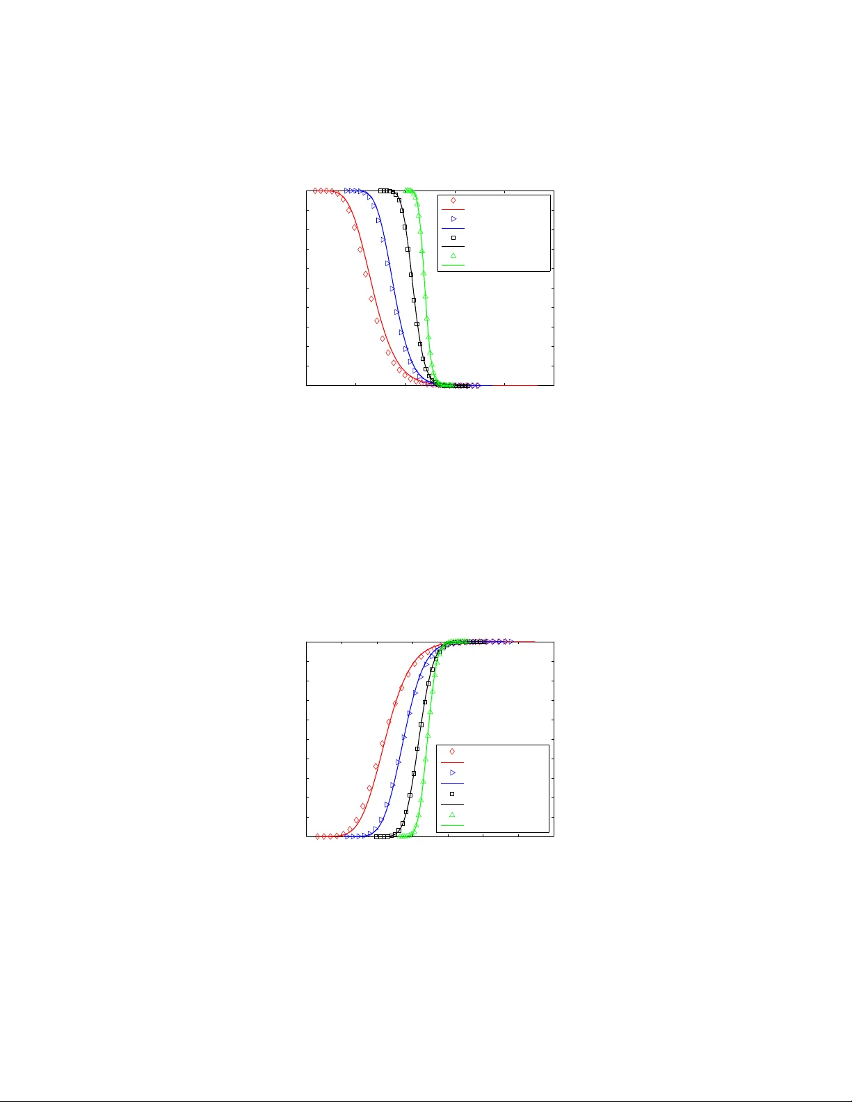
1 Theoretical Performance Analysis of Eigen v alue-based Detec tion Federico Penna, Student Member , IEEE, and R oberto Garello, Senior Member , IEEE Abstract In this paper we develop a complete analytical framework based on Random Matrix Theory for the perfor mance e valuation of Eigen value-based Detection. While, up to now , a nalysis was limited to false- alarm prob ability , w e have obtained an analytical expression also fo r the probab ility of missed detection, by using the theory o f sp iked po pulation mod els. A general scen ario with mu ltiple signals present a t the same time is considered . The theoretical results of this paper allow to predict the erro r pro babilities, and to set the d ecision thr eshold accord ingly , b y mean s of a few mathematical formu lae. In this way the design of an eig en value-based detector is made con ceptually identical to that of a trad itional energy detector . As add itional results, the paper discusses th e condition s of signal identifiability for single an d multiple sources. All th e ana lytical resu lts ar e validated through numerical simulations, covering also conv ergence, identifiabilty and non- Gaussian practical mod ulations. Index T erms Cognitive Radio, Spectrum Sensing, Random Matrix Theo ry , Spiked Population Models. I . I N T RO D U C T I O N Eigen value-based Detection (EBD) has been introduc ed [1], [2] as an e f ficient technique to perform spectrum se nsing in Cognitiv e Ra dio (CR). Using the EDB approach, the s econda ry re ceiv er is a ble to infer the prese nce or the abs ence o f a primary signal bas ed on the largest and the smallest eigenv alue of the rec eiv e d signal’ s covariance matrix. This techniqu e requires a coopera ti ve detection setting, wh ich may be a ccomplished by multiple antennas or coope ration among dif ferent use rs. In addition to the CR F . Penna is with TR M Lab - Isti tuto Superiore Mario Boella (ISMB) and with the Department of Electrical Engineering (DELEN), Politecnico di T orino, It aly . R. Garello is with the Department of Electrical Engineering (DELEN), Poli tecnico di T orino, Italy . e-mail: { federico.penna , roberto.garello } @polito.it. Nov ember 19, 2 021 DRAFT 2 context, the detec tion of signa l comp onents in noisy covari ance matrices is a very gen eral problem, with a wide v a riety of applications in c ommunications, statistics, gene tics, mathematical fin ance, a rtificial learning. The main ad vantage of fered by EDB is its robustness to the problem of n oise unce rtainty , which aff ects all the previously propose d detection schemes including the widely a dopted Energy Detection (ED). Howe ver , while for ED there exist co mprehens i ve the oretical results that allo w to express the error probabilities through analytical formulae, a corresponding theory for EBD has n ot bee n fully d ev eloped yet. In general, a signal detection sche me can be characterized b y defining two types of error probabilities: the probability of false alarm and t he probability of missed detection (see Sec. II-A f or a formal definition). These p robabilities de pend on the d ecision threshold (the value u sed by the algorithm to dec ide whether a signal is presen t o r ab sent). If ana lytical formulae a re av ailable, it is possible to: a) pr edict the e rror proba bilities of the s ystem a s a function of the decision threshold; b) set the decision thres hold a ccording to the required e rror con straints. Such formulae are well-known in c ase of ED. For EBD, up to no w , only a pproximated c riteria were proposed for the estimation of the false-alarm proba bility [1], [2] an d, to the bes t of ou r kn owledge, no exact analytical re sults hav e been fou nd for the missed-detection p robability y et. In this pa per , by exploiting the spectral properties of the sa mple cov a riance matri x und er the two complementary c onditions of signa l prese nt/absent, we derive an alytical express ions both for the false- alarm and the missed-de tection probability . The resu lt is a complete proba bilistic framework tha t allows to ev aluate the performance of EBD and to determine the proper decision threshold through analytical formulae. Whereas most of the works o n detection consider o nly the case of a single s ignal to be detected, our results also apply to the case of multiple p rimary signals. This generaliza tion is of interest for the applications in CR, since a sec ondary use r might be located in such a way as to hear diff erent primary signals (eac h with a different channel). The analytical resu lts derived in this p aper show that the numbe r of signals simultaneo usly present, as well as their powers and their channels, have an impact on the detection performance. The p aper is organized as follo ws: Se c II introduce s the signal mod el and the theoretical foundations of eigen value-base d detection; Sec. III and IV deri ve analytical results for the probabilities of false alarm and misse d detection, and for the signal iden tifiability condition; Sec. V discuss es the problem o f setting a proper decision threshold; Sec. VI validates the analys is throu gh numerical results; Sec. VII conclude s. Nov ember 19, 2 021 DRAFT 3 I I . E I G E N V A L U E - B A S E D D E T E C T I O N Notational remark: In the following, upper-case boldface letters indic ate matrices, lower -case bo ld- face letters ind icate vectors, the symb ols T and H indicate respec ti vely the transpo se a nd co njugate transpose (Hermitian) ope rators, tr( · ) is the trace o f a matrix, k · k is the Euclidea n n orm of a vector , diag( x ) indicates a square diagon al matrix whose main diagona l entries a re taken from the vector x , I N is the identity matrix (of size N if spec ified), 0 M ,N is a M × N matrix of zeros; the symbo l , stands for “de fined as”, the symb ol ∼ for “distributed with law”, a.s. − → indicates the almost su re con vergence, and D − → the con ver g ence in d istrib u tion; I { α } is the indicator function which takes value 1 where the condition α is true and 0 elsewhere. A. S ignal model W e cons ider a cooperative detection framework in which K receiv ers (or antennas ) collaborate to sense the s pectrum. Den ote with y k be the disc rete base band complex sample at rece i ver k , and d efine the K × 1 vector y = [ y 1 . . . y K ] T containing the K received s ignal sa mples. The g oal of the detector is to discriminate between two hypothese s: • H 0 (absenc e of primary signal). The samples contain on ly n oise: y | H 0 = v (1) where v ∼ N C ( 0 K, 1 , σ 2 v I K ) is a vector of circularly s ymmetric complex Gaus sian (CSCG) noise samples; • H 1 (presence of primary signal). For sake of gen erality , we consider a model whe re P primary signals may be simultaneous ly p resent: y | H 1 = H s + v (2) where: H is a K × P complex ma trix, where e ach element h k p represents the c hannel betwee n primary user p a nd receiver k (for simplicity , channe ls are ass umed to be memoryless and constant for the se nsing d uration); s is a P × 1 vector containing the primary s ignal samples, each coming from one of the P sources. The primary signa ls are assumed to be complex, z ero-mean and mutua lly independ ent with c ov ariance matrix E ss H , Σ = diag( σ 2 1 , . . . , σ 2 P ) (3) where σ 2 p is the variance of the p -th primary signal. Nov ember 19, 2 021 DRAFT 4 Under H 1 , w e define the signal-to-noise ratio (SNR) as ρ , E k H s k 2 E k v k 2 (4) This amo unts to ρ = tr H Σ H H K σ 2 v = P P p =1 σ 2 p k h p k 2 K σ 2 v (5) where h p is the p -th column of the matrix H , i.e., the ch annel vector referred to primary source p . In the single-us er cas e ( P = 1 ), we c an drop the index p and the express ion of the SNR simplifies to ρ | P =1 = σ 2 k h k 2 K σ 2 v (6) Remark: All througho ut this paper it is ass umed that P < K . When this assumption is n ot verified, the covari ance matrix lacks the necessa ry degrees of freedom to be able to distinguish the sign al components from the n oise. Notice tha t P might be u nknown, but to e nsure a reliable de tection K (which is a receiver parameter) ha s to be chosen g reater than the maximum possible numbe r of primary sign als. B. S pectral pr op erties of the s tatistical covar iance matrix Define the statistical covariance matrix of the received s ignal R , E y y H (7) Under H 0 and H 1 it is eq ual to, respec ti vely R = σ 2 v I K ( H 0 ) H Σ H H + σ 2 v I K ( H 1 ) (8) Let λ 1 ≥ . . . ≥ λ K be the eige n values o f R (without loss o f ge nerality , sorted in dec reasing orde r). Under H 0 , it is immediate to verify that λ i | H 0 = σ 2 v ∀ i = 1 , . . . , K (9) Under H 1 , there are ( K − P ) eigen values equal to σ 2 v and P greater , since H Σ H H is positive- semidefinite with rank P . The e igen values in this ca se can be written as λ i | H 1 = s i + σ 2 v (1 ≤ i ≤ P ) σ 2 v ( P < i ≤ K ) (10) where s 1 ≥ . . . ≥ s P > 0 deno te the P non-zero eige n values of the “signal cov ariance matrix” H Σ H H , and a re found by solving the cha racteristic equa tion det H Σ H H − s I K = 0 s.t. s 6 = 0 (11) Nov ember 19, 2 021 DRAFT 5 Becaus e of the ass umption P < K , the rank of the signal cov a riance matrix is P . It is po ssible to reduce the degree of the characteristic polynomial down to P by applying the ge neralized Matrix De terminant Lemma (MDL) [19] det H Σ H H − s I K = = det( Σ ) det( − s I K ) det Σ − 1 − 1 s H H H = = P Y p =1 σ 2 p ( − s ) K − P det H H H − s Σ − 1 (12) W e no te that the left-hand factor in (12) is a constan t with respe ct to s , the middle term gives rise to the ( K − P ) trivial solutions s = 0 , while the right-hand term d etermines the non -zero roots . The signa l eigen values s 1 , . . . , s P may there fore be calculated from the simplified characteristic eq uation det H H H − s Σ − 1 = 0 (13) which ha s degree P instead o f K . Since Σ is diagonal, Σ − 1 = diag ( σ − 2 1 , . . . , σ − 2 P ) . In the ca se of single pr imary use r ( P = 1) , there is o ne single signa l eigen value and, from (13), it has a very simple express ion: s 1 | P =1 = k h k 2 σ 2 (14) where the index ha s be en droppe d like in (6). The spectral p roperties o f R , summarized by (9) an d (10), motiv ate the adop tion of the ratio betwee n the lar gest a nd the s mallest e igen value of the covariance ma trix as a test statistic to discriminate betwee n the two hypothese s: under H 0 the ratio is equal to 1 , und er H 1 it is greater . Th is detec tion scheme was first p roposed in [1], [2]. C. S ample c ovariance matrix In pr actice, the statistical correlation matr ix R is estimated t hrough a sample c ovariance matrix . Introduce N as the number of s amples collecte d by e ach receiver during the se nsing period. It is as sumed that consec uti ve samples are uncorrelated and that all the random proces ses in volved (signals and noise) remain stationary for the s ensing duration. Then, let s ( n ) , v ( n ) and y ( n ) be, respecti vely , the transmitted signal vector , the noise vector and the rece i ved signa l vector at time n ; de fine the P × N ma trix S , [ s (1) . . . s ( N )] (15) Nov ember 19, 2 021 DRAFT 6 and the K × N matrices V , [ v (1) . . . v ( N )] (16) Y , [ y (1) . . . y ( N )] = H S + V (17) The K × K s ample c ov ariance matrix R ( N ) is then define d as R ( N ) , 1 N Y Y H (18) Denoting with ˆ λ 1 ≥ . . . ≥ ˆ λ K its eige n values, the test statistic used for detec tion is T , ˆ λ 1 ˆ λ K (19) Although R ( N ) con verges to R as N tends to infinity , for finite N its properties dep art from those of the statistical covariance matrix. In typical sensing ap plications N is expected to be quite large (to increase the detec tion reliability) but still not e normous (to reduce the s ensing time). W ith su ch re alistic values of N , the e igen values have no longer a deterministic be havior as in (8), but are characterized by a pr obability distribution . The refore the discrimination criterion ba sed on the eigen values is not as sharp-cutting as in the ideal case and may be affected by two possible error ev ents: false alarms and missed detections . Den oting with γ the dec ision threshold emp loyed by the detec tor , su ch tha t decision = H 0 if T < γ H 1 if T ≥ γ , the probability of false alarm may be express ed as P f a = Pr( T ≥ γ |H 0 ) (20) and the probability of miss ed d etection a s P md = Pr( T < γ |H 1 ) (21) These probabilities de pend on the distrib ution of T u nder the two hypo theses. The prob ability d istrib u tion function (PDF) and the cumulativ e distribution function (CDF) of T will be indicated as f T |H i ( t ) and F T |H i ( t ) , respectively , for i ∈ { 0 , 1 } . Thu s, (20) and (21) may be written a s P f a = 1 − F T |H 0 ( γ ) (22) P md = F T |H 1 ( γ ) (23) In the next se ctions the distrib ution of T in b oth ca ses will be de ri ved, using tools from Random Matrix Theory (RMT) which allow to analyze the s pectral prope rties of large-dimensional sample covariance Nov ember 19, 2 021 DRAFT 7 matrices. This makes it possible to ev alua te the dete ction pe rformance, giv en a decision thresh old, a s well as to express the threshold as a function of the requ ired probab ilities of false alarm or missed d etection (by in verting (22) and (23)). I I I . F A L S E - A L A R M P RO BA B I L I T Y A N A L Y S I S In this section, we first introduce so me useful results from RMT that exp ress the limiti ng distributi ons to which the lar g est and the smallest eigen values of R ( N ) con verge as N an d K grow . Then , we exploit these theoretical results to find the limiting distrib ution of the test statistic T and, through the relation (22), we derive the false-alarm proba bility . Most of the results of this se ction a lso appear , in a slightly diff erent form, in [21]. Here the results are s tated in their entirety an d are introduce d by a a more rigorous mathematical deriv ation. Also, a n ew notation is a dopted to emphas ize the link between the W ish art c ase ( H 0 ) a nd the spiked-pop ulation case ( H 1 , discu ssed in Sec. IV). A. R elevant r esults fr om Ran dom Matrix Theor y Under H 0 , since the columns of Y are zero-mea n indepe ndent comp lex Gauss ian vectors, the s ample covari ance matrix R ( N ) is a c omplex W ishar t ma trix [4]. The fluctuations of the eigen values of W is hart matrices have b een tho roughly in vestigated by RMT (see [3] and [6] for an o vervie w). The most remarkab le intuition of RMT is that in many cases the eigen values of matrices with random entries turn out to con verge to some fixed distrib ution, when both the d imensions of the s ignal matrix tend to infinity with the same order . For W ishart matrices the limiti ng joint eigen value distributi on has be en kn own for many years [5]; then, more recently , als o the ma r ginal distrib utions of sing le ordered eigen values have be en foun d. By exploiting some o f thes e results, we are ab le to express the asymptotical values of the largest and the sma llest eigen value of R ( N ) as well as their limiting distributions. W e s tate the following the orem, which s ummarizes a numbe r of rele vant results. Theorem 3.1 : Conver gence of the smallest and largest e igen values unde r H 0 . Let c , K N (24) and a ssume tha t for K, N → ∞ c → c ∈ (0 , 1) (25) Nov ember 19, 2 021 DRAFT 8 Define: µ ± ( c ) , c 1 / 2 ± 1 2 (26) ν ± ( c ) , c 1 / 2 ± 1 c − 1 / 2 ± 1 1 / 3 (27) Then, as N , K → ∞ , the following holds : (i) Almost s ure conver gence of the lar ges t e igen value ˆ λ 1 a.s. − → σ 2 v µ + ( c ) (28) (ii) Co n vergence in distributi on of the lar gest eigen v alue N 2 / 3 ˆ λ 1 − σ 2 v µ + ( c ) σ 2 v ν + ( c ) D − → W 2 (29) (iii) Almos t su r e con v erg ence of the s mallest eigen value ˆ λ K a.s. − → σ 2 v µ − ( c ) (30) (i v ) Co n ve r gen ce in distribution of the sma llest e igen value N 2 / 3 ˆ λ K − σ 2 v µ − ( c ) σ 2 v ν − ( c ) D − → W 2 (31) where W 2 is the T racy-W idom law of order 2, defined in Appen dix A. Pr oof: The c laims of this theorem follow from dif ferent results of RMT , up to some chan ges o f variables an d us ing a uniform notation. Proofs of the original theo rems a ppear in the references listed below . Claims (i) and (iii) des cend from the work by Marche nko and Pastur [5], later extended by Silverstein, Bai, Y in, et al. [6]. Claim (ii) was proved, unde r the a ssumption of Gauss ian e ntries, by Johan sson [7], J ohnston e [8] and Soshnikov [9], an d generalized to the non-Ga ussian case by P ´ ech ´ e [10]. Claim (iv) de ri ves from a very rece nt result by F eldheim a nd So din [11]. B. De rivation o f F T |H 0 and P f a The resu lts of The orem 3 .1 allow , through s ome algeb raic ma nipulations, to d etermine the limiting distrib ution of the test statistic T under the hypo thesis H 0 . Althoug h the resulting distrib ution is obtaine d under the joint limit K, N → ∞ , simulations s how that it provides an accurate estimation of the false- alarm p robability already for no t-so-lar ge values of K and N . Nume rical results inv e stigating this issu e are pres ented in Sec. VI. Nov ember 19, 2 021 DRAFT 9 In o rder to app ly claims (ii) a nd (iv), we define : L 1 , N 2 / 3 ˆ λ 1 − σ 2 v µ + ( c ) σ 2 v ν + ( c ) (32) L K , N 2 / 3 ˆ λ K − σ 2 v µ − ( c ) σ 2 v ν − ( c ) (33) For the above-mentioned theorem, bo th L 1 and L K con verge in d istrib u tion to the T racy-W idom law W 2 : f L 1 ( z ) , f L K ( z ) → f W 2 ( z ) (34) where f W 2 ( · ) represents the PDF associated w ith the law W 2 , a s de fined in Appen dix A. Then, from (19), the test s tatistic T b ecomes T = ˆ λ 1 ˆ λ K = N − 2 / 3 ν + ( c ) L 1 + µ + ( c ) N − 2 / 3 ν − ( c ) L K + µ − ( c ) (35) Notice tha t the term σ 2 v is cance led out in the ratio (this is the reaso n that makes the de tection thres hold “blind” with res pect to the noise power). W e deno te with l 1 and l K , respe cti vely , the numerator and the denominator of T , an d with f l 1 ( z ) and f l K ( z ) their limiting PDFs for N , K → ∞ . The se d istrib u tions are the same as those of L 1 and L K , u p to a linea r ran dom variable transformation: f l 1 ( z ) = N 2 / 3 ν + ( c ) f W 2 N 2 / 3 ν + ( c ) ( z − µ + ( c )) ! (36) For the denominator , it must be observed that ν − ( c ) < 0 for the c onsidered ran ge c ∈ (0 , 1) . Th us f l K ( z ) = N 2 / 3 | ν − ( c ) | f W 2 N 2 / 3 | ν − ( c ) | ( µ − ( c ) − z ) ! = − N 2 / 3 ν − ( c ) f W 2 N 2 / 3 ν − ( c ) ( z − µ − ( c )) ! (37) T o expres s the distributi on of T , we assume that f l 1 ( l 1 ) a nd f l K ( l K ) a re asymp totically independ ent, as it is reasonab le for the size of the covariance ma trix tending to infinity (and confirmed by follo wing numerical res ults): f l 1 ,l K ( l 1 , l K ) ≈ f l 1 ( l 1 ) f l K ( l K ) (38) Then, us ing the formula for the qu otient of random variables [20], the resulting ratio distributi on writes: f T |H 0 ( t ) = Z + ∞ −∞ | x | f l 1 ,l K ( tx, x ) dx · I { t> 1 } = Z + ∞ 0 x f l 1 ( tx ) f l K ( x ) dx · I { t> 1 } (39) Nov ember 19, 2 021 DRAFT 10 where the lower integration limit h as bee n ch anged to 0 instead of −∞ , since the c ov ariance matrix is positiv e -semidefinite therefore all the eige n values are non-negativ e; the con dition t > 1 is neces sary to preserve the o rder o f the eigenv alue s, s ince the distributi ons are de fined un der the ass umption l 1 > l K . Finally , we denote with F T |H 0 ( γ ) the CDF corresponding to (39). For N and K lar g e enou gh, we can approximate F T |H 0 ( γ ) , wh ich is need ed to comp ute P f a from (22), with the a symptotical dis trib ution: F T |H 0 ( γ ) ≈ F T |H 0 ( γ ) (40) The expression of F T |H 0 depend s on N and c , i.e ., N and K . Simulation results sh ow that the approxi- mation is ac curate for practical v alues of N and K , also q uite far from the asymp totical region. Clearly , the practical interest in the relation betwee n P f a and γ fou nd h ere is that it allows to determine the de cision thres hold as a fun ction of the required false-alarm probability; this application is disc ussed in mo re d etail in Sec. V. It is interesting to no te tha t the distrib u tion F T |H 0 for finite N a nd K can also be expres sed exactly , by following a comple tely dif ferent ap proach. This exact dis trib ution and the c orresponding detection threshold hav e been found in [22]. The drawback of the “exact” a pproach is its c omplexity , which makes implementation difficult whe n K and N are lar ge. I V . M I S S E D - D E T E C T I O N P RO B A B I L I T Y A N A LY S I S In this sec tion we use an approa ch based on RMT to deriv e the limiting distrib ution of T under H 1 and con seque ntly P md . As a preliminary step, we show that under this hypothe sis R ( N ) can b e reduce d to a so-ca lled spiked pop ulation model , i.e. , a model where the statistical c ovari ance matrix is a finite- rank perturbation of the identity . Spiked population models were introduc ed by John stone [8] a nd have an import ant role in Principal Component Analys is (PCA), with ma ny statistical applications ran ging from genetics to ma thematical finance . The fluctuations of the e igen values o f s ample cov a riance ma trices constructed from spiked mo dels a re nowadays a hot topic in RMT . A. R eduction to the Spiked P opulation Model Under H 1 , the received s ignal ma trix Y contains some Ga ussian entries, like in the W ishart case, along with a certain numbe r ( P ) of sign al components. In order to put into evidence the spiked structure of R ( N ) , the received signa l matrix Y (16) needs to be rewr itten in the form Y = T Z (41) Nov ember 19, 2 021 DRAFT 11 where T is a bloc k matrix of s ize K × ( P + K ) de fined as T = 1 σ v H Σ 1 / 2 I K (42) and Z , of size ( P + K ) × N , is defined a s Z = σ v Σ − 1 / 2 S V (43) This d ecompos ition ha s b een ch osen suc h that a ll the entries z ij of Z ( 1 ≤ i ≤ P + K, 1 ≤ j ≤ N ) have the follo wing properties: E z ij = 0 (44) E | z ij | 2 = σ 2 v (45) which a re n ecess ary c onditions for Theorem 4 .1 to hold. The covariance matrix becomes then R ( N ) = 1 N T Z Z H T H (46) which is exactly the model of [12], [13] and [14 ]. Finally , we deno te with t 1 , . . . , t K the eigen values of T T H . It follows from the structure of T tha t P e igen values a re diff erent from 1 (without los s of generality we put them in the first P pos itions: t 1 ≥ . . . ≥ t P ) and the rema ining K − P are ones. T o express the P “sp ike eige n values” (that represe nt the perturbation with respect to the pure-noise model), we notice that T T H = 1 σ 2 v H Σ H H + I K (47) and the eigen values t 1 , . . . , t P result from the solution of det H Σ H H − σ 2 v ( t − 1) I K = 0 s.t. t 6 = 1 (48) The structure of the problem is identical to that of (11), with the cha nge of v ariable s = σ 2 v ( t − 1) . W e can therefore c onclude that the “sp ike eige n values” t p are linked to the non-zero eigen values of the statistical c ov ariance matrix, s p , b y the relation t p = s p σ 2 v + 1 , 1 ≤ p ≤ P (49) In g eneral, the values of s p are calculated using (12); in the case of s ingle pr imary u ser ( P = 1 ), the re is the simplified expression (14) which lead s to t 1 | P =1 = k h k 2 σ 2 σ 2 v + 1 (50) Nov ember 19, 2 021 DRAFT 12 Relation between spike eigen v alues and SNR : The s pike eigen values are relate d with the SNR; this fact turns out to be useful espec ially in the case of P = 1 . From (49) we can write P X p =1 t p = 1 σ 2 v P X p =1 s p + P (51) but, from the eige ndecomp osition of H Σ H H and from (5) it follows that P X p =1 s p = tr H Σ H H = ρK σ 2 v (52) hence P X p =1 t p = K ρ + P (53) Therefore, in the case of one pr imary us er ( P = 1 ), the (uniqu e) s pike eige n value may b e expressed directly a s a function of the SNR: t 1 | P =1 = K ρ + 1 (54) Note that, by exploiting the property (52), one co uld also obtain (14) without resorting to the c haracteristic equation. In the case of multiple pr imary s ignals ( P > 1 ), the s um of the spike eigenv alues is related to the SNR, but not the single e igen values. Therefore, to compu te the t p (in particular t 1 , which is neede d to apply Theorem 4.1), it is nec essa ry to know the c hanne l matrix and the power of primary signals and use (13). B. R elevant r esults fr om Ran dom Matrix Theor y W e are now ready to state the follo wing the orem whic h provides a use ful result on the co n vergence of the largest eigenv alue in spiked population models . Theorem 4.1 : Conver gence of the lar gest eigen v alue unde r H 1 . A gain, ass ume that for K , N → ∞ c = K N → c ∈ (0 , 1) (55) In a ddition, as sume that for a ll i, j s. t. 1 ≤ i ≤ P + K , 1 ≤ j ≤ N : ( A 1 ) E z ij = 0 ( A 2 ) E ( ℜ z ij ) 2 = E ( ℑ z ij ) 2 = σ 2 v 2 ( A 3 ) ∀ k > 0 , E | z ij | 2 k < ∞ and E ( ℜ z ij ) 2 k + 1 = E ( ℑ z ij ) 2 k + 1 = 0 ( A 4 ) E ( ℜ z ij ) 4 = E ( ℑ z ij ) 4 = 3 4 σ 4 v Nov ember 19, 2021 DRAFT 13 Define: µ s ( t 1 , c ) , t 1 1 + c t 1 − 1 (56) ν s ( t 1 , c ) , t 1 q 1 − c ( t 1 − 1) 2 (57) Then, as N , K → ∞ , the following holds : (i) Almost s ure conver gence of the lar ges t e igen value: phase transition p henomen on If t 1 > 1 + c 1 / 2 : ˆ λ 1 a.s. − → σ 2 v µ s ( t 1 , c ) (58) If t 1 ≤ 1 + c 1 / 2 : ˆ λ 1 a.s. − → σ 2 v µ + ( c ) (59) (ii) Co n vergence in distributi on of the lar gest eigen v alue Let m (with 1 ≤ m ≤ P ) be the multiplicity of the first spike eigenv alue t 1 . If t 1 = . . . = t m > 1 + c 1 / 2 : N 1 / 2 ˆ λ 1 − σ 2 v µ s ( t 1 , c ) σ 2 v ν s ( t 1 , c ) D − → G m (60) If t 1 = . . . = t m = 1 + c 1 / 2 : N 2 / 3 ˆ λ 1 − σ 2 v µ + ( c ) σ 2 v ν + ( c ) D − → A m (61) If t 1 < 1 + c 1 / 2 : N 2 / 3 ˆ λ 1 − σ 2 v µ + ( c ) σ 2 v ν + ( c ) D − → W 2 (62) where A m and G m are distrib u tion laws defined in Appen dix B and C, respe ctiv e ly . Pr oof: The proof of claim (i) is due to Baik and Silverstein [12]; c laim (ii) was found by Baik, Ben A rous a nd P ´ ech ´ e [13] u nder the ad ditional ass umption of z ij Gaussian with u nit variance, and was generalized into this form by F ´ eral, P ´ ech ´ e [14] using res ults from Bai and Y ao [15]. C. Inter pr etation of the results 1) V alidi ty of the assum ptions: All the assumptions ( A 1 )-( A 4 ) are verified exactly for the noise part of Z , whose entries are comp lex Ga ussian random vari ables. For the signal part, the first two assu mptions are guarantee d by construction of Z : ( A 1 ) is giv en b y (44) an d ( A 2 ) is e quiv alen t to (45) (provided that the variance of s is equally distrib uted between real and imaginary pa rt, which is true for all type s o f complex signals used in communica tions). Assumption ( A 3 ) is also verified in practica l ca ses. Nov ember 19, 2021 DRAFT 14 Assumption ( A 4 ) is satisfied exa ctly by Ga ussian signa ls, wh ile there exist several types of sign als (e.g. P SK, QAM) whose fourt h moment is lo wer than that of a Gauss ian ran dom v ariable. Ho wever , since the type of primary signal is us ually un known to the seconda ry use rs, the Gaussian assumption is reasona ble in gene ral. In addition, since P < K , mo st of matrix Z is represented b y the noise part which does always satisfy ( A 4 ): therefore the theorem can be applied in almost a ll practical cases, ev en when this assump tion does no t hold exactly . The approximation introduce d in this way is s mall and become s negligible when the SNR of the primary signal is lo w , as s hown in Sec. VI-E. 2) Phase transition ph enomeno n: The first important result implied by the theorem is the existence of a critical va lue of t 1 that determines whethe r a signal co mponent is identifiable or no t. T his be havior is called phase transition phenomenon . In fact, when t 1 ≤ 1 + c 1 / 2 , the lar gest eigenv alue of the cov ariance matrix con verges to the same value as in the pure-noise model, whereas for t 1 > 1 + c 1 / 2 , it con verges to a larger value: µ s ( t 1 , c ) > µ + ( c ) . This prope rty makes it po ssible to detect the pres ence of signals. In c ase of P = 1 , the critical value c an be expressed directly in terms of the SNR using (54): ρ > 1 √ K N (63) This relation also allows to determine the minimum number o f samples for the de tector to be able to identify s ignals with a giv en SNR. 3) Limiting distributions: The s econd claim of the theorem c larifies how the largest e igen value con- ver g es to the asymptotical limit. For non-identifiab le componen ts, the limiting distributi on is the same as in the case of no signal. For c omponen ts with e igen values place d exactly on the criti cal point, the limiting distrib ution is a g eneralization of the o ne encoun tered in the p revious case: in fact, for m = 0 , A 0 reduces to the Tracy-W idom law (Appen dix B). For componen ts a bove the critical value, we find the distrib utions G m : for m = 1 , which is the most c ommon case in practical a pplications, G 1 is s imply the normal distributi on; for m = 2 , we have deriv ed a simple expression of the CDF of G 2 in terms of the Gaussian error function (see App endix C). Finally , notice that both the events o f eigen values exac tly equal to the critical point and of eige n values with multiplicity larger than o ne a re asy mptotically events with zero pr o bability . The res ults con cerning these case s are mentioned for comple teness, but are n ot important for practical applications. Therefore, the cas e (60) with G 1 is by far the most important result of this the orem and a llo ws to express P md . Furthermore, G 1 does not even inv olve comp licated ca lculations be cause it reduces to the Gaus sian distrib ution. Nov ember 19, 2021 DRAFT 15 D. De rivation o f F T |H 1 and P md Thanks to the results of The orem 4 .1, we are now ab le to exp ress the limiting probab ility distrib ution of the test statistic T un der the h ypothesis H 1 and, consequ ently , to de ri ve an ana lytical expres sion for the probability of missed detec tion. From now on, we refer to the case of identifiable signals , i.e., we assume the P s ignal co mponents p roduce sp iked e igen values above the critical limit 1 + c 1 / 2 . The a pproach tha t we adopt is the sa me as in the cas e of H 0 : we defi ne again L 1 , N 1 / 2 ˆ λ 1 − σ 2 v µ s ( t 1 , c ) σ 2 v ν s ( t 1 , c ) (64) which, for claim (ii), has a limiting P DF f L 1 ( z ) → f G m ( z ) (65) where f G m ( · ) rep resents the P DF a ssociated with G m ( m is the multiplicity of t 1 ), as defined in Appendix C. As for the distributi on of s mallest eige n value, we introduc e the following theorem. Theorem 4.2 : Distribution of the K − P smallest eigen v alues under H 1 . Assume tha t for K, N → ∞ c = K N → c ∈ (0 , 1) (66) and that t p > 1 + c 1 / 2 for 1 ≤ p ≤ P , the eige n values ˆ λ P +1 , . . . , ˆ λ K of R ( N ) have asymptotically the same limiti ng distributi on as tho se o f a ( K − P ) × ( K − P ) W ishart matrix. Pr oof: The resu lt follows from the p roof of Lemma 2 in [16]. Therefore, the distribution of the smallest eige n value is not a f fected by the presence of “s pikes” and claims (iii) and (i v ) of Theo rem 3. 1 can be applied also in this case with the only difference that, instead of c (24), now c ′ = K − P N (67) Thus, we defi ne L K , N 2 / 3 ˆ λ K − σ 2 v µ − ( c ′ ) σ 2 v ν − ( c ′ ) (68) which s till co n verges in distribution to the T racy-W idom law f L K ( z ) → f W 2 ( z ) (69) Then the tes t statistic T be comes T = ˆ λ 1 ˆ λ K = N − 1 / 2 ν s ( t 1 , c ) L 1 + µ s ( t 1 , c ) N − 2 / 3 ν − ( c ′ ) L K + µ − ( c ′ ) (70) Nov ember 19, 2021 DRAFT 16 Also in this ca se the noise variance σ 2 v is can celed ou t in the ratio. Howe ver , an implicit d epende nce on σ 2 v remains in the term t 1 , exc ept for the case of s ingle primary us er ( P = 1 ) wh ere t 1 is a func tion o f the SNR only (54). W e d enote with l 1 and l K , respe cti vely , the numerator and the denominator of T an d with f l 1 ( z ) and f l K ( z ) their limiting PDFs for N , K → ∞ . Through a random v ariable transformation, they may be expressed as f l 1 ( z ) = N 1 / 2 ν s ( t 1 , c ) f G m N 1 / 2 ν s ( t 1 , c ) ( z − µ s ( t 1 , c )) ! (71) f l K ( z ) = N 2 / 3 | ν − ( c ′ ) | f W 2 N 2 / 3 | ν − ( c ′ ) | ( µ − ( c ′ ) − z ) ! (72) Notice that, as a conse quence of the obse rvati ons in IV - B, G m is with prob ability o ne a Gaus sian distrib ution a nd thu s it can be written in a mo re p ractical form as f l 1 ( z ) = ( N/ 2 π ) 1 / 2 ν s ( t 1 , c ) exp − N 2 ν 2 s ( t 1 , c ) ( z − µ s ( t 1 , c )) 2 (73) Also in this case, we as sume f l 1 ( l 1 ) and f l K ( l K ) as asymptotically inde pende nt. The resu lting limi ting ratio distributions is f T |H 1 ( t ) = Z + ∞ −∞ | x | f l 1 ,l K ( tx, x ) dx · I { t> 1 } = Z + ∞ 0 x f l 1 ( tx ) f l K ( x ) dx · I { t> 1 } (74) where, like in the previous ca se, the d omain of integration ha s bee n restricted to n on-negativ e values, and the cond ition t > 1 is nec essary to ensure that l 1 > l K . Finally , denoting with F T |H 1 ( γ ) the CDF co rresponding to the PDF in (74), we can take the approx- imation F T |H 1 ( γ ) ≈ F T |H 1 ( γ ) (75) that, in the asymptotica l limit for N and K , is the expression of the misse d detection probability as it is giv e n by (23 ). Nu merical res ults sh ow that the a pproximation is quite a ccurate for all cases o f prac tical interest. The relation be tween P md and γ allows to predict the missed -detection proba bility of the detector with a giv en threshold, or to express the decision threshold as a function of the req uired probability of missed detection. The proble m of setting the threshold is discusse d in more d etail in the next sec tion. Nov ember 19, 2021 DRAFT 17 V . S E T T I N G T H E D E C I S I O N T H R E S H O L D The results prese nted in the previous se ctions expres s P f a and P md as a function of γ ; therefore, by in verting the relations (22) and (23 ), the thresh old can be express ed as a function of the error probabilities. A. T hr eshold as a func tion of P f a The fi rst relation γ ( P f a ) = F − 1 T |H 0 (1 − P f a ) (76) allows to se t the dec ision thres hold accurately even if the no ise power ( σ 2 v ) is unk nown, since F T |H 0 depend s only on the number of rec eiv ers ( K ) an d of samples ( N ). Th e thres hold s et in this way , as a function of a target P f a , is therefore a “ blind’ d ecision sche me as it is insens iti ve both to the noise and to the sign al power . In a previous work, Zeng an d Liang [2] propose d a similar ap proach to set the decision thresho ld a s a function of the prob ability of false alarm. Their de tection a lgorithm was ba sed o n an approx imated distrib ution of T , c alculated taking into acco unt only the limiti ng distrib ution of the largest eige n value (Theorem 3.1(ii)), and therefore provides non -optimal detection pe rformance. In [1] anothe r e igen value- based detection sche me was proposed , base d only on the asy mptotical values of ˆ λ 1 and ˆ λ K (Theorem 3.1(i)(i ii)). For this reason, it do es not allow to ad just the thresho ld as a fun ction of P f a and is s trongly sub-optimal with resp ect to our s cheme un less N a nd K a re extremely lar ge. A de tailed performance co mparison between the threshold based on the limiting distrib ution F T |H 0 and the se two previous a pproache s was p rovided in [21]. B. T hr eshold as a func tion of P md The s econd rela tion is γ ( P md ) = F − 1 T |H 1 (1 − P md ) (77) Whereas γ ( P f a ) has b een found to dep end only on K and N , the expression of γ ( P md ) depends also on the characteristics of the signal to be detected . In particular , tw o ca ses have to be con sidered separately: • when P = 1 , the only additional pa rameter n eeded to co mpute P md is the SNR ρ . In this case, the detector may still be defined “ blind” since it do es n ot n eed to know explicitly the noise power nor the signal p ower . (Clearly , the detec tion performanc e ha s to be related, at least, with the SN R. Nov ember 19, 2021 DRAFT 18 For instance, in the case of Ene r gy De tection, the SNR a nd the noise power are ne eded to c ompute P md .) • when P > 1 , the knowledge of additional parameters is needed , name ly the noise power ( σ 2 v ), the number of p rimary us ers ( P ), their powers ( σ 2 1 , . . . , σ 2 P ), and the ch annel ( H ). These depende nces arise from the nonlinea r expression of t 1 (48). In general, all the se pa rameters (even the SNR an d the potential numbe r of primary users) might be unknown. The refore, the relation betwee n γ and P md should b etter be used in the forw ard way , to predict the P md achieved using a g i ven thresh old under the possible primary signa l s cenarios, rather tha n to set the decision threshold according to a tar ge t P md . Nevert heless, i f the system imposes a certain requirement on P md to kee p the interference caus ed by the sec ondary network below a maximum level, the formula is use ful to determine γ based on the worst-case sce nario (i.e., the on e with the h ighest missed-detec tion probability) s o as to guarantee in all case s the required protection to the primary network. C. Co mplexity and prac tical implementation As shown in [2] a nd [21], eigenv alue-ba sed d etection schemes offer a substantial performance im- provement compared to ED (and a complete protection to noise uncertainty) at the price o f a n increa sed complexity . Most of the co mputational complexity of these algo rithms deri ves from the co mputation of the covariance matrix and of its eige n values: in [2] it is e stimated that such operations lead to a comp lexity that grows as K 3 , wh ereas in the cas e of ED it g rows linea rly with K . This increased c omputational cost is not d ramatic, since the numbe r o f rece i vers is never eno rmous. On the other ha nd, in terms of the sample n umber (which is, ac tually , very large) the complexity remains linear with N for both EBD and E D. Howe ver , it is important to remark tha t the computationa l complexity is not influence d by the com- putation o f the thresho ld. Even if the formulae foun d in this paper to express the threshold are very complex, they are a lw ays implemen ted off-l ine, and what the detector uses is simply a look-up table (LUT) c ontaining several values of γ as a function of N , K P f a , an d/or P md and SNR. The use of LUTs also allows to cha nge the decision threshold “on the fly ”, in cas e of modifications of the system requirements. Finally , for the comp utation of the distribution functions defined in this p aper , routines are av ailable on the we b (e.g. , [18] for the Tr acy-W idom distributi ons) or ca n be implemented directly from the d efinitions giv e n in the Ap pendice s. Nov ember 19, 2021 DRAFT 19 V I . N U M E R I C A L R E S U L T S In this sec tion, the results de ri ved analytically in the previous sec tions a re validated by comparing them with e mpirical results, ob tained from Matlab Mon te-Carlo simulations. The parameters use d in the simulations are described in ea ch s ub-section; when referring to the SNR, it is defined acco rding to (4). A. Distr ibut ion of T unde r H 0 Figure 1 represe nts the probability of false a larm, i.e., the co mplementary CDF of T und er H 0 , for N = 1000 and d if feren t values of K (i.e., of c ). The value of σ 2 v has no ef fect, as it gets ca nceled out in the test statistic. The c urve predicted u sing the an alytical express ion turns out to be consisten t with the empirical data in all the cons idered c ases. Comparing the three curves obtained with diff erent values o f K , one may observe that for a giv e n γ the prob ability o f false alarm increases with K . However , this does not mean that the detector performance worsens for lar ger K , bec ause also the c urve of P md shifts rightwards, and conseq uently the de cision thres hold. The overall effect is ind eed an improvement of pe rformance wh en K gets lar ger , as expected intuiti vely . B. Distr ibut ion of T unde r H 1 Figures 2, 3 and 4 s how the probability of misse d d etection, i.e., the CDF of T under H 1 , for the same v alues of N and K as in the previous case . The entries of H are taken as zero-mean complex Gauss ian random coef ficients (Rayleigh fading), with a vari ance normalized so as to obtain the desired SNR. In the first figu re the SNR is − 10 dB with P = 1 primary signa l; in the sec ond one, the SNR is − 20 dB again with P = 1 ; in the third one, P = 2 with a global SNR o f − 10 dB (from (5) with: ρ 1 = σ 2 1 k h 1 k 2 K σ 2 v = 0 . 06 ≈ − 12 . 2 d B; ρ 2 = σ 2 2 k h 2 k 2 K σ 2 v = 0 . 04 ≈ − 14 . 0 dB; σ 2 v = 1 ). Notice tha t in the last ca se ( P > 1 ) the lar gest spike eigenv alue t 1 , which determines P md , depend s on all the entries of H and not only on the SNR. In our s imulations t 1 = { 2 . 25 , 4 . 04 , 7 . 60 } , respectively for K = { 20 , 50 , 100 } . Also in this ca se, the analytical c urves fit the e mpirical d ata well in all the co nsidered c ases. W e have considered lo w values of SNR, since the low-SNR region is the most important both from the the oretical point of view ( t 1 close to the critical value of iden tifiability) and from the prac tical point of v iew (the challenge for cogn iti ve radios is to detect sign als also in pres ence of fading or shad owing). Nov ember 19, 2021 DRAFT 20 As previously mentioned, the curves o f P md shift rightwards as K increases , i.e. , the missed-detection probability gets lower for a given γ . This f a ct compensates the increa se of P f a resulting in a larger separation be tween 1 − F T |H 0 and F T |H 1 for larger K . C. Co n vergence Figures 5 an d 6 s how the c on vergence of the empirical CDFs to the analytical CDFs, which are calculated under asy mptotical assumptions for N and K . Four dif feren t couples of { N , K } have been considered while keeping the ir ratio c fixed at 0 . 1 . Remarkab ly , even though the CDFs are asymp totical they provide an accu rate approximation of the empirical C DFs als o for low K and N . In the case H 0 , as N and K increase the CDF tend s to a step function, b ecause the largest an d the smallest eigen values con verge (almost surely) to the values µ + ( c ) and µ − ( c ) , respectiv ely; the variance instead depends also on N (it g ets s maller for larger N ). For the case H 1 , we cons idered a scenario with P = 1 a nd, to make the compa rison mo re evident, we kept t 1 fixed instea d of the SNR ( ρ and t 1 are linked by a factor K , s o they can not remain both constant with different K ). In particular we c hose the value t 1 = 2 , which is above the c ritical value that is 1 + √ c = 1 . 3162 for a ll the c onsidered couples of { N , K } . Similarly as in the p revious case, the CDFs turn out to conv er ge to a ste p function correspond ing to the almost s ure as ymptotical limits of the eigen values. D. Ide ntifiability As a result of the pha se transition ph enomeno n of Theorem 4.1, signals be low a certain power le vel are no t identifiable. A d etection limit as a func tion of the SNR is expressed by the relation (63), valid for P = 1 . F igure 7 represen ts graph ically the critical SNR for de tection as a func tion of the number of samples N a nd of receiv ers K . The relation may be use d to determine the minimum s ensing duration (i.e., the minimum number of s amples) need ed to detect s ignals for a req uired detector se nsiti vity . A relation be tween identifiability thresho ld and SNR is vali d only for P = 1 . For multiple s ignals, the expression of t 1 is more complex and does no t de pend o nly on the SNR. Howev er , it turns out that also for P > 1 the value of t 1 is d etermined essen tially by the power of the lar g est signal, i.e., by the SNR as if the first c omponent was alone. T herefore, we may define an app roximated expression of the SNR, similar as (6), depen ding o nly on the power of the dominant signal comp onent: ρ ≈ max p σ 2 p k h p k 2 K σ 2 v (78) Nov ember 19, 2021 DRAFT 21 This express ion can b e use d in (63) to determine, app roximately , the para meters N and K of the detector . As an example, in fig ure 8 we consider the case P = 2 with ρ 1 fixed at 0 . 1 = − 10 dB and ρ 2 varying from 0 and ρ 1 . T he g raph sh ows t 1 as a func tion of ρ 2 , c omparing the cas e whe n t 1 is c alculated from the exac t formula for P = 2 (11) with the case when it is c alculated taking into acco unt the lar gest compone nt only (78) and with the case of a s ingle compone nt, but with doub le power (SNR = 2 ρ 1 ). It turns ou t that the ac tual value of t 1 is very close to the a pproximated one, even when the sum of ρ 1 and ρ 2 is c lose to 2 ρ 1 . F urthermore, the app roximated t 1 tends to und erestimate the a ctual t 1 , re sulting in a conservati ve choice of N and K . E. No n-Gaussian s ignals As pointed out in Sec. IV -B, the last assumption o f Thereom 4.1 is often not satisfied in practice, since realistic signals hav e typ ically a fourth moment lower than that of a Gau ssian ran dom variable. Figures 9 and 10 show how the theo retical results, which rely o n that assu mption, fit empirical data obtaine d using more realistic types of primary s ignal. W e considered four dif feren t typ es of signals, all with the same variance as in the Gaussian case, but with dif ferent fourth moments. The first curve refers to a 4-PSK modulated primary sign al, with ideal rectang ular pulse-shap e filter a nd assuming a cohe rent reception; in the second curve, the sign al is the same but pas sed through a square root rais ed cosine (SRRC) filter with roll-of f α = 0 . 5 ; the third curve is a PSK s ignal with non-coheren t reception (i.e., eac h sample has a rand om phas e); the last cu rve refers to a ra ndom comp lex signal whose real and imaginary parts are uniformly distributed. In the first figure, when the SNR is very low ( − 20 dB), the theoretical distribution fits the empirical data pe rfectly in spite of the fourth moment o f the signa ls. When the SNR increase s ( − 10 dB), so me dif ference between the theoretical and the empirical curve can be observed, esp ecially for PSK s ignals. It is interesting to notice that the Gaussian ap proximation on the fou rth moment af fects the varianc e of the resulting distribution, but not the me an . The result is that the an alytical formula overestimates the probability of misse d detection (the interes ting pa rt of the c urve is for P md < 0 . 5 , i.e ., the left tail). T o obtain a more ac curate estimation of the miss ed-detection prob ability in cas e of no n-Gaussian signals, for h igh SNR, one s hould add a “c orrection coef ficient” to the theoretical v ariance ν s ( t 1 , c ) . Such coefficients would depend on the fourth moment of the signa ls, σ 4 p , and would b e therefore specific of the modu lation u sed. It might be possible to determine by simulation the correction coefficients for a particular signal as a fun ction of the SNR, wh ereas de termining them analytically is a more challenging task sinc e the matrix Z is c ompose d of heterog eneous entries. Ho wever , the Gaussian as sumption is v alid Nov ember 19, 2021 DRAFT 22 asymptotically for ρ → −∞ (the sign al pa rt in Z becomes negligible) and is accurate enou gh in the low- SNR region as s hown by figure 9. F . R eceiver ope rating cha racteristics (R OC) Figures 11 and 12 repres ent the p erformance of the eigen value-based detector in the form of comple- mentary R OC (receiv er ope rating charac teristics), i.e., P md as a function o f the target P f a . The curves are plotted by setting the thres hold as a function of the false-alarm proba bility and deriving the c orresponding missed-detec tion p robability f or that threshold. The graphs compare the curves obtained from the empirical distrib utions with those obtained using the ana lytical expres sions of this pape r: (76) to se t γ ( P f a ) , then (23) to compu te P md ( γ ) . The first R OC graph refers to the same scenario as figures 1 (for P f a ) and 3 (for P md ), with N = 100 0 and K = 50 ; the secon d one refers to the s cenario of figure 4 (for P md ) with the sa me values of N a nd K . The overall detector performance exp ressed by the R OC improv es a s the separation b etween the P f a curve (monotonica lly decrea sing) and the P md curve (monotonica lly increas ing) gets lar g er , thus letting both P f a and P md be n early zero for a wide range of γ . Such distan ce increa ses with K , N and with the SNR. For this reason , in the se cond R OC the performanc e is almost idea l (zero P md for all the P f a ). In the first R OC on the con trary there are finite missed-detec tion probab ilities for the c onsidered range of P f a ; the ana lytical result also in this case turns ou t to be consistent with the empirical da ta. V I I . C O N C L U S I O N In this pape r , ana lytical formulae have been fou nd for the limiting distribution of the ratio between the largest and the smallest eigenv alue in sample covariance matrices , either constructed from pure -noise (W ishart) models o r s ignal-and-noise (spiked population) mode ls. Th ese results have b een ap plied to the problem of signal detection (in particular , in the c ontext of Cognitive Ra dio), wh ere e igen value-base d detection has proved to be an efficient technique . Among the main results of the pa per , there are the an alytical formulation of the missed detec tion probability as a function of the threshold, and the deriv a tion an d discuss ion of sign al identifiability conditions. All the results have been validated via nume rical simulations c overing f als e-alarm and missed - detection vs. threshold, con vergence behavior , ide ntifiability for single and multiple primary users as a function of the SNR, validity of the approac h for realistic modulated s ignals, ROC curves. Nov ember 19, 2021 DRAFT 23 A P P E N D I X A. T racy -W idom d istributi on The T racy-W ido m d istrib u tions W 2 were introduced in [17], to express the distrib u tion o f the la r gest eigen value in a Gau ssian Unitary Ensemb le (GUE). De fine the complex Airy function, Ai ( u ) = 1 2 π Z ∞ e jπ / 6 ∞ e 5 jπ / 6 e j ua + j 1 3 a 3 da (79) the Airy kernel, A ( u, v ) = Ai ( u ) Ai ′ ( v ) − Ai ′ ( u ) Ai ( v ) u − v (80) and let the A x be the operator a cting on L 2 (( x, + ∞ )) wi th kernel A ( u, v ) . The n, the se cond-order T racy-W idom CDF , F W 2 ( x ) , is d efined in terms o f the Fredh olm determinant F W 2 ( x ) = d et(1 − A x ) (81) It also admits an alternati ve expres sion. Let q ( u ) be the solution of the Painlev ´ e II differential equation q ′′ ( u ) = uq ( u ) + 2 q 3 ( u ) (82) satisfying q ( u ) ∼ − Ai ( u ) , u → + ∞ (83) Then F W 2 ( x ) = exp − Z + ∞ x ( u − x ) q 2 ( u ) du (84) Notice that this de finition, and the index 2 , are referred to the case of co mplex Gaus sian v ariables. In the case of real signals, one should u se the co rresponding first-order T racy-W idom distrib u tion [17]. B. A iry-type d istributi ons These d istrib u tions are d efined in [13] as a n extens ion of the T racy-W idom (GUE) distrib ution. L et s ( m ) ( u ) = 1 2 π Z ∞ e jπ / 6 ∞ e 5 jπ / 6 e j ua + j 1 3 a 3 1 ( j a ) m da (85) t ( m ) ( u ) = 1 2 π Z ∞ e jπ / 6 ∞ e 5 jπ / 6 e j ua + j 1 3 a 3 ( j a ) m − 1 da (86) Then, for k ≥ 1 , the CDFs of A k are defined a s F A k ( x ) = d et(1 − A x ) · (87) · det δ mn − < 1 1 − A x s ( m ) , t ( n ) > 1 ≤ m,n ≤ k Nov ember 19, 2021 DRAFT 24 where < , > is the real inne r prod uct of functions in L 2 (( x, + ∞ )) . For k = 0 , this distrib ution reduces to the GUE distrib u tion: F A 0 ( x ) = F W 2 ( x ) (88) For k = 1 , it can be written in the Painlev ´ e form F A 1 ( x ) = F W 2 ( x ) exp Z + ∞ x q ( u ) du (89) C. Fi nite GUE distributions The distrib utions G k are defined in [13 ] as the distribution o f the largest e igen value in a k × k G UE. Their CDF is F G k ( x ) = (2 π ) − k / 2 k Y m =1 m ! ! − 1 · (90) · Z x −∞ . . . Z x −∞ Y 1 ≤ m
Original Paper
Loading high-quality paper...
Comments & Academic Discussion
Loading comments...
Leave a Comment