Performance of Hybrid-ARQ in Block-Fading Channels: A Fixed Outage Probability Analysis

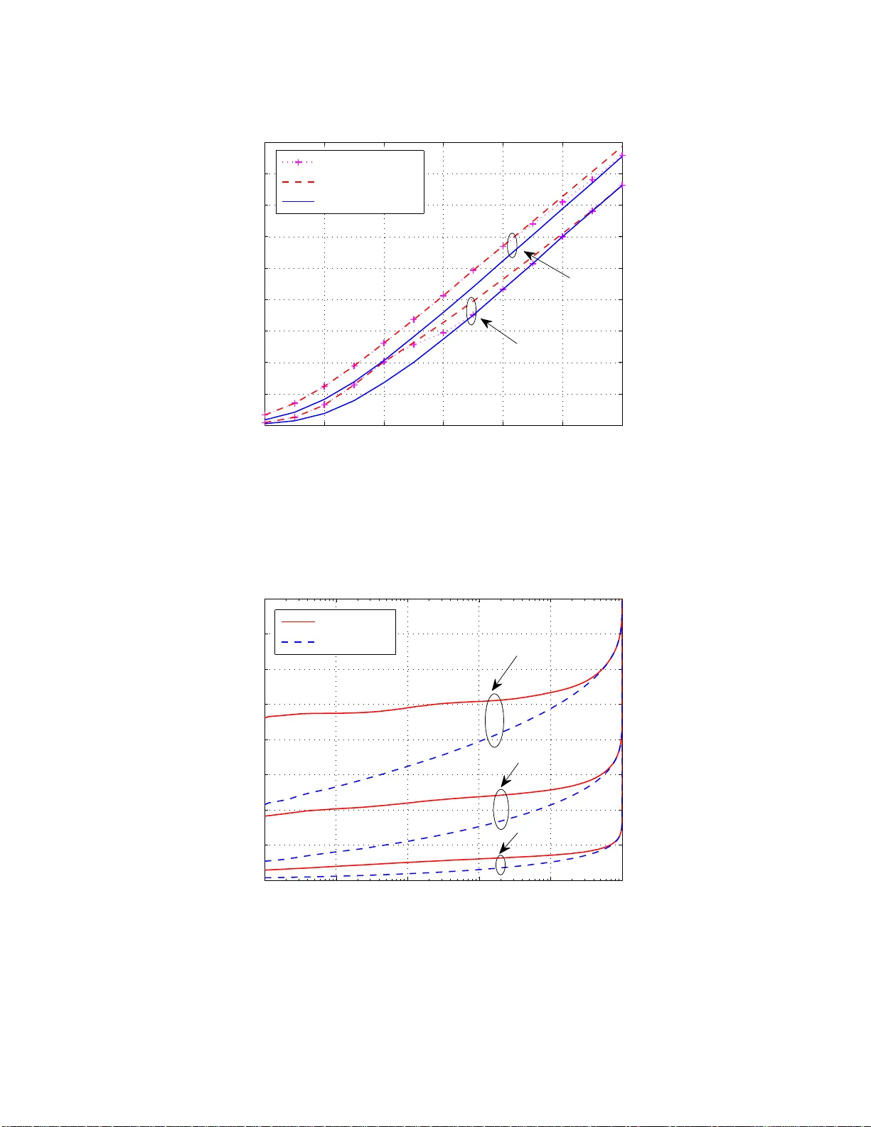
1 Performance of Hybrid-ARQ in Block-F ading Channels: A Fix ed Outage Probability Analysis Peng W u and Nihar Jindal Abstract This paper studies the perf ormance of hybrid -ARQ (automatic repeat request) in Rayleigh blo ck- fading channels. T he long- term av erage tran smitted rate is an alyzed in a fast-fading scena rio where th e transmitter only has knowledge of ch annel statistics, and, consistent with contem porary wire less systems, rate adaptatio n is per formed such that a target o utage prob ability (after a m aximum num ber of H -ARQ round s) is main tained. H-ARQ allows for ea rly ter mination on ce dec oding is possible, and thus is a coarse, a nd imp licit, mech anism fo r rate adaptation to the instantan eous chann el quality . Alth ough th e rate with H-ARQ is not as large as the ergodic capacity , which is achievable with rate adaptation to the instantaneou s chann el co nditions, even a few ro unds of H-ARQ make the gap to ergo dic capa city reasonably small f or op erating points o f interest. Fur thermor e, the rate with H- ARQ provid es a significant advantage compare d to systems that do not use H-ARQ and only adapt rate based on t he channel statistics. I . I N T RO D U C T I O N ARQ (automatic repeat reques t) is an extremely p owerful type o f fee dback-ba sed communica tion that is e xtensively used at dif feren t layers o f the network stack. The basic ARQ strategy a dheres to the pattern of t ransmission followed by feedba ck of an A CK/N A CK to indica te su ccess ful/unsucces sful dec oding. If simple ARQ or hybr id -ARQ (H-ARQ) with Ch ase combining (CC) [1] is use d, a N A CK leads to retransmission of the same p acket in the second ARQ round. I f H-ARQ with incremental r edunda ncy (IR) is used, the second transmission is not the same as the first and ins tead contains some “new” information regarding the mes sage (e.g., ad ditional pa rity bits). After the sec ond round the rece i ver again attempts to de code, b ased upon the s econd AR Q roun d alone (simple ARQ) or upon both ARQ rounds (H-ARQ, either CC or IR). The transmitter moves on to the next mes sage when the rece i ver correctly decode s a nd se nds bac k an A CK, or a max imum number of ARQ round s (per mess age) is reac hed. ARQ provides an ad vantage by allo wing for early termination once s ufficient information has been receiv ed. As a result, it is most u seful when there is co nsiderably uncertainty in the amou nt/quality The authors are with the Department of Electrical and Computer Engineering, Uni versity of Minnesota, Minneapolis, MN 55455, USA (email: pengwu@umn.edu; nihar@umn.edu). October 23, 2018 DRAFT 2 of information re ceiv ed. At the network layer , this might c orrespond to a s etting where the n etwork conges tion is unknown to the transmitter . At the phys ical laye r , which is the focus of this paper , this correspond s to a fading ch annel whos e instantaneo us quality is unk nown to the trans mitter . Although H-ARQ is widely used in co ntemporary wireless systems such as HSP A [2], W iMax [3] (IEEE 802 .16e) and 3 GPP L TE [4], the majority of res earch on this topic has focused o n code design , e.g., [5], [6], [7], while relatively litt le research has focuse d on performance analys is of H-ARQ [8]. Most relev ant to the pres ent work, in [9] Ca ire a nd T unine tti esta blished a relationsh ip b etween H-ARQ throughput an d mutua l information in the limi t of infinite block length. For multi ple antenna syste ms, the div ersity-multiplexing-delay trade off o f H-ARQ was studie d by El Gama l e t a l. [10 ], a nd the c oding scheme ac hieving the op timal trade off was introduced; C huang et al. [11] con sidered the optimal SNR exponent in the bloc k-fading MIMO (multiple-input multiple-output) H-ARQ chann el with disc rete input signal con stellation satisfying a sh ort-term power constraint. H-ARQ has also b een rec ently studied in quasi-static cha nnels (i.e., the cha nnel is fixed over all H-ARQ rounds) [12], [13] and sho wn to bring benefits to sec recy [14]. In this paper we build upon the results of [9] and perform a mutua l information-bas ed analys is of H- ARQ in block-fading ch annels. W e c onsider a scena rio where the fading is too fast to a llo w ins tantaneous channe l quality feedbac k to the transmitter , a nd thus the trans mitter only has knowledge of the chann el statistics, but nonetheles s each transmiss ion experiences on ly a limited d egree of ch annel selec ti vity . In this setting, rate ad aptation ca n o nly be pe rformed ba sed on chann el statistics and achieving a reason able error/outage probab ility generally requires a conservati ve choice of ra te if H-ARQ is not used . On the other hand , H-ARQ allows for implicit rate ada ptation to the instantan eous ch annel q uality beca use the receiv er terminates transmission once the c hannel conditions expe rienced by a codeword are goo d en ough to a llo w for deco ding. W e a nalyze the long-term average trans mitted rate achieved with H-ARQ, assuming that there is a maximum number of H-ARQ rounds and that a target o utage p robability a t H-ARQ termination cann ot be exc eeded. W e compare this rate to tha t a chieved withou t H-ARQ in the same se tting as w ell a s to the e r godic capacity , which is the a chiev a ble rate in the idealized setting where instantaneous cha nnel information is avail able to the transmitter . The main findings of the pap er a re that (a) H-ARQ gene rally provides a significant adv a ntage over systems that d o not use H-ARQ but ha ve an equi valent level of channe l s electivity , (b) the H-ARQ rate is reas onably close to the er go dic capacity in ma ny practical settings, an d (c) the rate with H-ARQ is much less s ensitiv e to the desired outage proba bility than an equiv a lent s ystem tha t does not us e H-ARQ. October 23, 2018 DRAFT 3 The prese nt work d if fers from prior literature in a n umber of important a spects. One key distinction is that we consider systems in whic h the r ate is adapted to t he av erage SNR such that a con stant tar ge t outage probability is maintained at all SNR’ s, whereas most prior work has cons idered e ither fixed rate (and thus decreas ing outage ) [11] or increas ing rate and de creasing ou tage as in the di versity-multiple xing trade off framew o rk [10][15]. The fixed outage paradigm is con sistent with contemporary wireless s ystems whe re an outag e lev e l ne ar 1 % is typ ical (see [16] for discu ssion), a nd certain con clusions depen d heavily on the outage ass umption. W ith respect to [9], no te tha t the focus of [9] is on multi-user issues, e .g., whether or not a system b ecomes interf erence-limited at high SNR in the regime of very large dela y , whereas we c onsider single-user s ystems and g enerally focus on p erformance with short delay constraints (i.e., maximum n umber of H-ARQ round s). In a ddition, we use the attempted transmission rate, rather than the suc cessful rate (which is used in [9]), as our p erformance metric. This is moti vated by applications such as V oice-over -IP (V oIP), where a packet is dropp ed (an d n ever retransmitted) if it cannot be decod ed after the maximum number of H-ARQ rounds and quality of service is maintained by achieving the target (post-H-ARQ) outage probability . On the other hand, reliable data c ommunication requires the use o f higher-l ayer retransmissions whenever H-ARQ outag es occur; in such a s etting, the relev ant metric is the succe ssful rate, which is the product of the a ttempted transmission rate and the s ucces s probab ility (i.e., one minus the post-H-ARQ outag e probability). If the post-H-ARQ o utage is fi xed to some target value (e.g., 1% ), then studying the a ttempted rate is effecti vely equiv a lent to s tudying the succ essful rate. 1 I I . S Y S T E M M O D E L W e co nsider a block-fading ch annel where the channel remains constant ov er a block b ut varies independ ently from one block to another . The t -th received symbol in the i -th b lock is given by : y t,i = √ SNR h i x t,i + z t,i , (1) where the index i = 1 , 2 , · · · indicates the block nu mber , t = 1 , 2 , · · · , T indexes c hanne l us es within a block, SNR is the average recei ved SNR, h i is the fading cha nnel coefficient in the i -th b lock, and x t,i , y t,i , and z t,i are the transmitted symbo l, re ceiv ed s ymbol, and ad diti ve noise, res pectiv ely . It is assume d that h k is complex Gaussian (circularly symmetric) with u nit variance and z ero me an, and that h 1 , h 2 , . . . are i.i.d.. T he no ise z t,i has the s ame d istrib u tion as h k and is indepen dent a cross c hanne l us es a nd bloc ks. 1 If th e post-H-ARQ outage probability can be optimized, then a careful balancing between the attempted rate and higher-layer retransmissions should be conducted in order t o maximize the successful r ate. Although this is beyon d the scope of the present paper , note that some results in this direction can be found in [17 ] [18]. October 23, 2018 DRAFT 4 The transmitted sy mbol x t,i is con strained to have unit average power; we co nsider Gaussian inputs, and thus x t,i has the same d istrib u tion a s the fading and the noise. Althou gh we foc us only on Rayleigh fading and single antenna systems, our basic insights can be extende d to inc orporate other fading distributions and MIMO a s discu ssed in Section IV (Remark 1). W e consider the setting where the receiv e r h as perfect c hannel state i nformation (CSI), while the transmitter is aware of the channel d istrib u tion b u t d oes no t k now the ins tantaneous c hannel qu ality . This models a s ystem in which the fading is too fast to a llo w for feedb ack of the instantane ous ch annel conditions from the receiver b ack to the transmitter , i.e ., the cha nnel co herence time is not much lar ger than the delay in the feedba ck loop. In cellular systems this is the case for moderate-to-high velocity users. This setting is often referred to as ope n-loop bec ause of the lac k o f instantaneou s channe l tracking at the transmitter , a lthough other forms of feedbac k, su ch a s H-ARQ, are permitted. The relevant performance metrics, n otably wh at we refer to as outage probability an d fixed ou tage transmitted rate, are spe cified at the beginning of the relev an t s ections. If H-ARQ is not used , we a ssume eac h cod ew o rd s pans L fading bloc ks; L is the refore the cha nnel selectivity expe rienced by ea ch codeword. Whe n H-ARQ is used, we ma ke the following as sumptions: • The chan nel is constan t within eac h H-ARQ round ( T symbols), but is indepen dent acros s H-ARQ rounds. 2 • A maximum of M H-ARQ round s are a llo wed. An outag e is dec lared if de coding is not po ssible after M rounds, an d this outage p robability c an be no lar ger than the con straint ǫ . Becaus e the ch annel is assu med to be independ ent across H-ARQ rounds, M is the ma ximum a mount of channe l selec ti v ity experienced by a co dew ord. Whe n comparing H-ARQ and no H-ARQ, w e set L = M such that maximum selec ti v ity is equalized. It is worth noting tha t the se assumptions on the ch annel v a riation are quite re asonab le for the fast- fading/open-loop sce narios. Transmission slots in modern systems are typically arou nd one millisecond, during which the channel is rough ly con stant even for fast fading. 3 An H-ARQ round generally cor - 2 An intuitiv e but some what misleading extension of the quasi-static fading model to the H-ARQ setting is to assume that the channel is constant for the duration of the H-ARQ rounds corresponding to a particular message/code word, but is drawn independe ntly across different messages. Because more H-ARQ rounds are needed to decode when the channel quality i s poor , such a model actually changes the underlying fading distribution by increasing the probability of poor states and reducing the probability of good channel states. In this light, it is more accurate model the channel across H-ARQ rounds according to a stationary and ergodic random process with a high degree of correlation. 3 Frequency -domain channel v ariation within each H-ARQ round is briefly discussed in Section IV -B. October 23, 2018 DRAFT 5 responds to a s ingle transmission slot, but su bseque nt ARQ rounds are sepa rated in time by at l east a few slots to a llo w for deco ding a nd A CK/NA CK feedba ck; thus the assu mption of inde penden t channe ls across H-ARQ rou nds is rea sonable. Moreover , a constraint o n the n umber of H-ARQ rounds limits complexity (the de coder must retain information rec eiv ed in prior H-ARQ rounds in memory) and delay . Throughou t the paper we use the notation F − 1 ǫ ( X ) to denote the solution y to the equ ation P [ X ≤ y ] = ǫ , where X is a rando m variable; this q uantity is well defined wh erev er it is us ed. I I I . P E R F O R M A N C E W I T H O U T H - A R Q : F I X E D - L E N G T H C O D I N G W e begin by s tudying the baseline scen ario where H-ARQ is not used and every c odeword spans L fading blocks. In this setting the o utage probability is the proba bility that mutual i nformation received over the L fading blocks is smaller than the transmitted rate R [19, eq (5.83)]: P out ( R, SNR ) = P " 1 L L X i =1 log 2 (1 + SNR | h i | 2 ) ≤ R # . (2) where h i is the channe l in the i -th fading block. The ou tage probability reasonably approximates the decoding error probability for a sys tem with strong cod ing [20] [21], a nd the achiev ability of this error probability h as been rigorously shown in the limit of infinite block length ( T → ∞ ) [22] [23]. Becaus e the outage proba bility is a non -decreasing function of R , by s etting the outage probability to ǫ a nd s olving for R we g et the following straightforward defi nition of ǫ -outage c apacity [24]: Definition 1: The ǫ -outa ge capacity with outage constraint ǫ and di versity order L , denoted by C L ǫ ( SNR ) , is the largest rate such tha t the ou tage probability in (2) is no larger than ǫ : C L ǫ ( SNR ) , max P out ( R, SNR ) ≤ ǫ R (3) Using no tation introduc ed earlier , the ǫ -outage capa city c an b e rewritt en as C L ǫ ( SNR ) = F − 1 ǫ 1 L L X i =1 log 2 (1 + SNR | h i | 2 ) ! (4) = log 2 SNR + F − 1 ǫ 1 L L X i =1 log 2  1 SNR + | h i | 2  ! . (5) For L = 1 , P out ( R, SNR ) can be written in closed form and in verted to yield C 1 ǫ ( SNR ) = log 2  1 + log e  1 1 − ǫ  SNR  [19]. For L > 1 the o utage probability cann ot be written in close d form nor in verted, and therefore C L ǫ ( SNR ) must b e numerically computed. Th ere are, however , two us eful approximations to ǫ -outag e capac ity . The fi rst one is the high-SNR af fine approximation [25], which ad ds a cons tant rate off set term to the sta ndard multiplexing gain characterization. October 23, 2018 DRAFT 6 Theorem 1: The high-SNR af fine app roximation to ǫ -outage capac ity is given by C L ǫ ( SNR ) = log 2 SNR + F − 1 ǫ 1 L L X i =1 log 2  | h i | 2  ! + o (1) , (6) where the no tation implies that the o (1) term vanishes a s SNR → ∞ . Pr oof: The proof is identical to that of the high-SNR of fse t c haracterization of MIMO channels in [26, Theorem 1], noting that single antenna bloc k fading is e quiv alen t to a MIMO chan nel wit h a diagonal cha nnel matrix. In terms of standard high SNR notation where C ( SNR ) = S ∞ (log 2 SNR − L ∞ ) + o (1) [25][27], the multiplexing gain S ∞ = 1 and the rate offset L ∞ = − F − 1 ǫ  1 L P L i =1 log 2  | h i | 2   . The rate of fse t is the difference be tween the ǫ -outage c apacity and the capa city of an A WGN chan nel with signa l-to-noise ratio SNR . Although a closed form expres sion for L ∞ cannot be found for L > 1 , from [28], P " 1 L L X i =1 log 2  | h i | 2  ≤ y # = 2 y L G L, 1 1 ,L +1  2 y L | 0 0 , 0 ,..., 0 , − 1  , (7) where G m,n p,q  x | a 1 ,...,a p b 1 ,...,b q  is the Meijer G-function [29, eq. (9.301)]. Bas ed o n (6), L ∞ therefore is the solution to 2 −L ∞ L G L, 1 1 ,L +1  2 −L ∞ L | 0 0 , 0 ,..., 0 , − 1  = ǫ . The rate offset L ∞ is plotted versus L in Fig. 1 for ǫ = 0 . 01 . As L → ∞ the offset c on verges to − E [log 2  | h | 2  ] ≈ 0 . 83 , the offset of the ergodic Rayleigh channe l [27 ]. While the affine approximation is acc urate at high SNR’ s, moti vated by t he Central Limit Theorem (CL T), an approximation that is more accurate for moderate and low SNR’ s is rea ched by a pproximating random variable 1 L P L i =1 log 2 (1 + SNR | h i | 2 ) by a Gauss ian random variable with the same mea n and variance [30][31]. The mean µ and variance σ 2 of log 2 (1 + SNR | h | 2 ) are given by [32][33]: µ ( SNR ) = E [log 2 (1 + SNR | h | 2 )] = log 2 ( e ) e 1 / SNR E 1 (1 / SNR ) , (8) σ 2 ( SNR ) = 2 SNR log 2 2 ( e ) e 1 / SNR G 4 , 0 3 , 4  1 / SNR | 0 , 0 , 0 0 , − 1 , − 1 , − 1  − µ 2 ( SNR ) , (9) where E 1 ( x ) = R ∞ 1 t − 1 e − xt dt , and at high SNR the standard deviation σ ( SNR ) con ver g es to π log 2 e √ 6 [33]. The mutua l information is thus a pproximated by a N ( µ ( SNR ) , σ 2 ( SNR ) L ) , and therefore P out ( R, SNR ) ≈ Q √ L σ ( SNR ) ( µ ( SNR ) − R ) ! , (10) where Q ( · ) is the tail p robability of a unit variance no rmal. Setting this quantity to ǫ and then s olving for R y ields an ǫ -outage capac ity a pproximation [30, eq . (26)]: C L ǫ ( SNR ) ≈ µ ( SNR ) − σ ( SNR ) √ L Q − 1 ( ǫ ) . (11) October 23, 2018 DRAFT 7 The ac curacy of this ap proximation d epends on how a ccurately the CDF of a Gau ssian ma tches the CDF (i.e., outage probability) of random variable 1 L P L i =1 log 2 (1 + SNR | h i | 2 ) . In F ig. 2 both CDF’ s are plotted for L = 2 and L = 10 , an d SNR = 0 , 10 , an d 20 dB. A s expec ted by the CL T , as L increa ses the approximation b ecomes more accurate. Furthermore, the match is less accurate for very small values of ǫ becaus e the tails of the Gaussian a nd the actual random variable d o not p recisely match. Finally , n ote tha t the match is not as acc urate at low SNR’ s: this is be cause the mu tual information random variable h as a density close to a c hi-square in this regime, and is thu s not well approx imated by a Gaus sian. Although not accura te in all regimes, numerical results confirm that the Gaussian approximation is reasona bly accurate for the range of i nterest for parameters (e.g. , 0 . 01 ≤ ǫ ≤ 0 . 2 and 0 ≤ SNR ≤ 2 0 dB). More importantly , this app roximation yields important ins ights. In Fig. 3 the true ǫ -outag e cap acity C L ǫ ( SNR ) a nd the affine and Gauss ian approximations are plotted versus SNR for ǫ = 0 . 01 a nd L = 3 , 10 . T he Gauss ian approximation is reaso nably accurate at moderate SNR’ s, and is more accurate for larger values of L . On the other h and, the affine a pproximation, which provides a correct high SNR off set, is as ymptotically tight at h igh S NR. A. Er go dic Capacity Gap When ev a luating the eff ect of the diversity order L , it is useful to c ompare the ergodic c apacity µ ( SNR ) and C L ǫ ( SNR ) . By Chebysh ev’ s ine quality , for any 0 < w < µ , P "      µ ( SNR ) − 1 L L X i =1 log 2 (1 + SNR | h i | 2 )      ≥ w # ≤ σ 2 ( SNR ) Lw 2 (12) By replacing w with µ ( SNR ) − R a nd equa ting the right h and side (RHS) with ǫ , we get µ ( SNR ) − σ ( SNR ) √ Lǫ ≤ C L ǫ ( SNR ) ≤ µ ( SNR ) + σ ( SNR ) √ Lǫ . (13) This implies C L ǫ ( SNR ) → µ ( SNR ) as L → ∞ , as intuiti vely expec ted; reasona ble values o f ǫ are smaller than 0 . 5 , and thus we expect con vergence to occ ur from below . In order to ca pture the speed at which this c on vergence occ urs, we d efine the quantity ∆ EC − FD as the dif ference between the ergodic and ǫ -outage capac ities. Based on (13) we ca n uppe r bound ∆ EC − FD as: ∆ EC − FD ( SNR ) = µ ( SNR ) − C L ǫ ( SNR ) ≤ σ ( SNR ) √ Lǫ . (14) This boun d shows that the rate g ap goes to zero at least as fast a s O  1 / √ L  . Althoug h we ca nnot rigorously claim tha t ∆ EC − FD is of order 1 / √ L , by (11) the Gauss ian a pproximation to this quantity is: ∆ EC − FD ( SNR ) ≈ σ ( SNR ) √ L Q − 1 ( ǫ ) , (15) October 23, 2018 DRAFT 8 which is also O  1 / √ L  . This approximation become s more acc urate as L → ∞ , by the CL T , a nd thu s is expe cted to correctly cap ture the sc aling w ith L . No te that (15 ) has the interpretation tha t the rate must be Q − 1 ( ǫ ) √ L deviations below the e r godic capacity µ ( SNR ) in order to ensure 1 − ǫ reliability . In Fig. 4 the actual c apacity g ap a nd the app roximation in (15) are plotted for ǫ = 0 . 01 and ǫ = 0 . 05 with SNR = 20 dB, an d a reaso nable match be tween the approx imation and the exact ga p is seen . I V . P E R F O R M A N C E W I T H H Y B R I D - A R Q W e no w move on to the a nalysis of hybrid-ARQ, which will be shown t o provide a significa nt performance advantage relative to the baseline of n on-H-ARQ performance . H-ARQ is clearly a variable- length code, in which c ase the average transmiss ion rate must be suitably defined. If each message contains b information bits an d ea ch A RQ round c orresponds to T channel symbols, the n the initial transmission rate i s R init , b T bits/symbol. If random v a riable X i denotes the number of H-ARQ rounds used for the i -th messag e, then a total of P N i =1 X i H-ARQ rounds are used and the average transmission rate (in bits/symbol or bps/Hz ) across those N mes sages is: N b T P N i =1 X i = R init 1 N P N i =1 X i . (16) W e are interes ted in the long-term average transmission ra te, i.e., the cas e where N → ∞ . By the law of lar ge numbers (no te that the X i ’ s are i.i.d. in our mod el), 1 N P N i =1 X i → E [ X ] and thus the rate con verges to R init E [ X ] bits/symbol (17) Here X is the random v a riable representing the number of H-ARQ rounds per message; this ran dom variable is de termined by the sp ecifics of the H-ARQ protocol. In the remainder of the pap er we focus on incremental redundancy (IR) H-ARQ becaus e it is the most powerful type of H-ARQ, although we compare IR to Chase co mbining in Sec tion IV -E. In [9] it is shown that mutual information is ac cumulated over H-ARQ rounds whe n IR is used, an d that dec oding is pos sible once the accu mulated mutual information is larger than the numb er of information bits in the messag e. Th erefore, the numb er of H-ARQ roun ds X is the smallest nu mber m such that: m X i =1 log 2 (1 + SNR | h i | 2 ) > R init . (18) The n umber of rounds is up per boun ded by M , a nd a n outag e occurs whe never the mutua l information after M round s is smaller than R init : P IR ,M out ( R init ) = P " M X i =1 log 2 (1 + SNR | h i | 2 ) ≤ R init # . (19) October 23, 2018 DRAFT 9 This is the s ame as the exp ression for outage proba bility o f M -order diversit y without H-ARQ in (2), except tha t mutual information is summed rather than averaged over the M rounds. This dif ference is a conseq uence o f the fact that R init is de fined for trans mission over o ne round rather tha n a ll M rounds; divi ding by E [ X ] in (17) to obtain the a verage trans mitted rate makes the exp ressions consistent. Due to this relations hip, if the initial rate is s et as R init = M · C M ǫ , where C M ǫ is the ǫ -outage capa city for M -order diversity withou t H-ARQ, then the outage at H-ARQ termination is ǫ . In order to simplify express ions, it is useful to defin e A k ( R init ) as the probability that the accumu lated mutual information after k rounds is smaller tha n R init : A k ( R init ) , P " k X i =1 log 2 (1 + SNR | h i | 2 ) ≤ R init # . (20) The expe cted number of H-ARQ rounds per mes sage is therefore gi ven by: E [ X ] = 1 + M − 1 X k =1 P [ X > k ] = 1 + M − 1 X k =1 A k ( R init ) . (21) The long-term average transmitted rate, which is denoted as C IR ,M ǫ , is defin ed by (17). W ith init ial rate R init = M · C M ǫ we have: 4 C IR ,M ǫ , R init E [ X ] =  M E [ X ]  C M ǫ . (22) Note that C IR ,M ǫ is the attempted long-term average transmission rate, as dis cussed in Section I. For the sake of brevit y this quantity is re ferred to as the H-ARQ rate; this is n ot to be c onfused with the initial rate R init . S imilarly , we refer to ǫ -outage cap acity C M ǫ as the no n-H-ARQ rate in the res t of the p aper . Becaus e E [ X ] ≤ M , the H-ARQ rate is at least as lar ge as the non -H-ARQ rate, i.e., C IR ,M ǫ ≥ C M ǫ , and the ad vantage with respect to the non -H-ARQ benc hmark is p recisely the multiplicati ve factor M E [ X ] . This diff erence is explained as follows. Be cause R init = M · C M ǫ , each mess age/pac ket co ntains C M ǫ M T information bits regardless of whether H-ARQ is us ed. W ithou t H-ARQ these bits are always transmitted over M T symbols, w hereas with H-ARQ an average of o nly E [ X ] T s ymbols are required. In Fig. 5 the average rates with ( C IR ,M ǫ ) and without H-ARQ ( C M ǫ ) are plotted versus SNR for ǫ = 0 . 01 and M = 1 , 2 and 6 ( M = 1 does no t allow for H-ARQ in ou r model). Ergodic ca pacity is also plotted as a referen ce. Base d on the figu re, we immediately notice: • H-ARQ with 6 rounds outperforms H-ARQ with 2 rounds. 4 All quantities in this expression except M are actually functions of SNR . For the sake of compactness, howe ver , dependence upon SNR is suppressed in this and subsequent expressions, excep t where explicit notation is necessary . October 23, 2018 DRAFT 10 • H-ARQ provides a significa nt a dvantage relative to non-H-ARQ for the same value of M for a wide range o f SNR’ s, but this a dvantage vanishes at high SNR. Increasing rate with M is to be expected, beca use lar g er M correspond s to more time di versity an d more early termination opportunities. The beha vior wit h respect t o SNR is perhap s les s intuiti ve. The remainder o f this section is dev o ted to quantifying and explaining the behavior se en in Fig. 5. W e begin by extending the Gaussian a pproximation to H-ARQ, then examine performance s caling with respect to M , SNR , and ǫ , a nd fin ally c ompare IR to Ch ase C ombining. A. Gaussian Approximation By the defi nition of A k ( · ) a nd (21)-(22), the H-ARQ rate c an be written as: C IR ,M ǫ = A − 1 M ( ǫ ) 1 + P M − 1 k =1 A k  A − 1 M ( ǫ )  , (23) where A − 1 M ( · ) refers to the in verse of function A M ( · ) . If we us e the approach of Section III and approximate the mutual information accu mulated in k rounds by a Gaussian with mean µk and variance σ 2 k , where µ and σ 2 are defi ned in (8) and (9 ), we have: A k ( R init ) ≈ Q  µk − R init σ √ k  . (24) Similar to (11), the initial rate R init = A − 1 M ( ǫ ) can be ap proximated a s M h µ − σ √ M Q − 1 ( ǫ ) i . App lying the approximation of A k ( R init ) to eac h term in (23 ) an d using the p roperty 1 − Q ( x ) = Q ( − x ) yields: C IR ,M ǫ ≈ M h µ − σ √ M Q − 1 ( ǫ ) i M − P M − 1 k =1 Q  M − k √ k µ σ − q M k Q − 1 ( ǫ )  . ( 25) This approximation is easier to compute than the actual H-ARQ rate and is reas onably a ccurate. Further - more, it is useful for the insights it can p rovide. B. Scaling with H-ARQ Rounds M In this section we study the depen dence of the H-ARQ rate on M . W e first show con vergence to the ergodic capacity as M → ∞ : Theorem 2: For any SNR , the H-ARQ rate c on verges to the ergodic capac ity a s M → ∞ : lim M → ∞ C IR ,M ǫ ( SNR ) = µ ( SNR ) (26) Pr oof: See Ap pendix A. October 23, 2018 DRAFT 11 T o quantify how fast this co n vergence is, similar to Se ction III-A we in vestigate the d if fere nce b etween the er godic c apacity an d the H-ARQ rate. Defin ing ∆ EC − IR , µ ( SNR ) − C IR ,M ǫ ( SNR ) w e have ∆ EC − IR = µ E [ X ]  E [ X ] − M · C M ǫ µ  ≈ µ E [ X ]  E [ X ] −  M − σ µ Q − 1 ( ǫ ) √ M  (27) where the approximation follo ws from C M ǫ ≈ µ − σQ − 1 ( ǫ ) √ M in (11). Becaus e E [ X ] is on the order of M (as established in the proof of T heorem 2), the key is the behavior of the term E [ X ] −  M − σ µ Q − 1 ( ǫ ) √ M  . T o better und erstand E [ X ] we a gain return to the Gaussian approximation. Whil e the CDF of X i s defined by P ( X ≤ k ) = 1 − A k ( R init ) (for k = 1 , . . . , M − 1 ), we use ˜ X to denote the random variable using the Gauss ian approximation and thus de fine its CDF (for integers k ) a s: P  ˜ X ≤ k  = Q µ ( M − k ) − √ M σ Q − 1 ( ǫ ) σ √ k ! (28) where we have use d A k ( R init ) ≈ Q  µk − R init σ √ k  ev alua ted with R init = M C M ǫ ≈ M µ − √ M σ Q − 1 ( ǫ ) . From this expression , we can immediately see tha t the median of ˜ X is l M − σ µ Q − 1 ( ǫ ) √ M m [34]. If this was equ al to the mean of X , then by (27) the rate difference would b e well app roximated by β µ M , where β is the difference betwee n l M − σ µ Q − 1 ( ǫ ) √ M m and  M − β µ Q − 1 ( ǫ ) √ M  and thu s is n o larger tha n one. By studying the characteristics o f ˜ X (and of X ) we can see that the med ian is in fact quite c lose to the mea n. A tedious c alculation in Appe ndix B giv e s the following ap proximation to E [ X ] : E [ X ] ≈ M − σ µ Q − 1 ( ǫ ) √ M + 0 . 5(1 − ǫ ) − σ µ √ M Z ∞ Q − 1 ( ǫ ) Q ( x ) dx, (29) which is reasona bly acc urate for large M . The mos t important factor is the te rm 0 . 5(1 − ǫ ) , which is due to the fact tha t o nly a n integer nu mber of H-ARQ rounds c an be use d. The factor − σ µ √ M R ∞ Q − 1 ( ǫ ) Q ( x ) dx exists beca use the rand om variable is truncated at the point where its CDF is 1 − ǫ . Applying this into (27), the rate d if feren ce can be a pproximated as: ∆ EC − IR ≈ µ  0 . 5(1 − ǫ ) − σ µ √ M R ∞ Q − 1 ( ǫ ) Q ( x ) dx  M − σ µ Q − 1 ( ǫ ) √ M − σ µ √ M R ∞ Q − 1 ( ǫ ) Q ( x ) dx + 0 . 5(1 − ǫ ) . (30) The de nominator increases with M at the order of M (more precisely a s M − √ M ), while the numerator actually dec reases with M and can even b ecome negativ e if M is extremely large. For reaso nable values of M , howev er , the nega ti ve term in the numerator is es sentially incons equential (for example, if ǫ = 0 . 01 and SNR = 10 dB, the n egati ve term i s much smaller than 0 . 5(1 − ǫ ) for M < 5000 ) a nd thus can be reasona bly neglected. By igno ring this negati ve term and replacing the den ominator with the leading order M term, we get a further app roximation of the rate gap : ∆ EC − IR ≈ 0 . 5(1 − ǫ ) µ M (31) October 23, 2018 DRAFT 12 Based on this ap proximation, we see that the rate gap decrea ses roughly on the orde r O (1 / M ) , rathe r than the O  1 / √ M  decreas e without H-ARQ. In Fig. 6 we plot the exact c apacity gap with a nd without H-ARQ, as well as the Gaussian approximation to the H-ARQ gap (30) and its simplified form in (31 ) for ǫ = 0 . 0 1 at SNR = 10 dB. Both a pproximations are seen to be reasonab ly ac curate especially f or lar ge M . In the ins et p lot, which is in log-log sca le, we see tha t the exact ca pacity ga p goe s to z ero at order 1 / M , co nsistent with the result ob tained from our approximation. The f as t conv er gence with H-ARQ c an be intuiti vely explained as follo ws. If transmission could be stopped precisely when e nough mu tual information has be en recei ved, the transmitted rate would be exactly matched to the insta ntaneous mutual information an d thus ergodic ca pacity would be achieved. When H-ARQ is used , howe ver , trans mission ca n only be terminated a t the end of a roun d as, oppos ed to within a round, and thus a small amount of the transmission can b e wasted. Th is ”rounding error”, which is reflected in the 0 . 5(1 − ǫ ) term in (30) and (31), is essentially t he only penalty incurred by using H-ARQ rather than explicit rate adaptation. Remark 1: Beca use the value o f H-ARQ depend s primarily on the mean an d variance of the mutual information in ea ch H-ARQ roun d, our basic insights can b e extended to multiple-antenn a channe ls and to c hannels w ith freque ncy (or time) div e rsity within eac h ARQ round if the c hange in mea n an d variance is ac counted for . For example, with order F frequen cy diversity the mutua l information in the i -th H- ARQ round become s 1 F P F l =1 log(1 + SNR | h i,l | 2 ) , wh ere h i,l is the chan nel in the i -th round on the l -th frequency chann el. The mean mutual information is unaffected, while the vari ance is decreas ed by a factor of 1 F . ♦ C. Scaling with SNR In this section we qua ntify the be havior of H-ARQ a s a function o f the average SNR. 5 Fig. 5 indicated that the be nefit of H-ARQ vanishes at high SNR, a nd the follo wing theorem makes this precise: Theorem 3: If SNR is taken to infinity wh ile keep ing M fixed, the expected number of H-ARQ rounds co n verges to M and the H-ARQ rate c on verges to C M ǫ ( SNR ) , the non-H-ARQ rate wit h the 5 Because constant ou tage corresponds to the full-multiple xing point, the results of [10] imply that C IR ,M ǫ cannot have a multiplexing gain/pre-log larger t han one (in [10] it is shown that H-ARQ does not increase t he full multiplexing point). Ho we ver , the DMT -based results of [10] do not provide rate-offset characterization as in Theorems 3 and 4. October 23, 2018 DRAFT 13 same selectivity: lim SNR →∞ E [ X ] = M (32) lim SNR →∞  C IR ,M ǫ ( SNR ) − C M ǫ ( SNR )  = 0 (33) Pr oof: See Ap pendix C. The intuition b ehind this res ult can be gathered from Fig. 7, where the CDF’ s of the accumulated mutual information a fter 2 a nd 3 rounds are p lotted for for SNR = 10 a nd 40 d B. If M = 3 the initial rate is set at the ǫ -point of the CDF of P 3 i =1 log(1 + SNR | h i | 2 ) . Becau se the CDF’ s overlap for M = 2 and M = 3 considera bly wh en SNR = 10 dB, there is a lar ge probability tha t s ufficient mutua l information is accumu lated a fter 2 rounds and thus early termination oc curs. Ho wever , the overlap between t hese CDF’ s disap pears as SNR increases , bec ause P k i =1 log(1 + SNR | h i | 2 ) ≈ k log SNR + P k i =1 log( | h i | 2 ) , and thus the ea rly termination probability vanishes . Although the H-ARQ advantage eventually vanishes, the a dvantage persists thr oughou t a lar ge SNR range an d the Gaussian approx imation (Sec tion IV -A) can b e used to quantify this. The probability o f terminating in strictly less than M roun ds is approximated by: P [ X ≤ M − 1] ≈ Q µ ( SNR ) − √ M σ ( SNR ) Q − 1 ( ǫ ) σ √ M − 1 ! (34) In orde r for this approximation to b e grea ter than one -half we require the numerator inside the Q -func tion to be less than z ero, which correspo nds to µ ( SNR ) σ ( SNR ) ≤ √ M Q − 1 ( ǫ ) or √ M ≥ µ ( SNR ) σ ( SNR ) Q − 1 ( ǫ ) (35) As SNR increases µ ( SNR ) increases without bou nd where as σ ( SNR ) c on verges to a co nstant. Th us µ ( S NR ) /σ ( SNR ) increases quickly with SNR , which makes the proba bility o f ea rly termination vanish. From this we se e that the H-ARQ advantage lasts longer ( in terms of SNR ) whe n M is larger . The second i nequality in (35) c aptures a n alternati ve viewpoint, which is roughly the minimum value of M required for H-ARQ to provide a sign ificant ad vantage. Moti vated b y na i ve intuition that the H-ARQ rate is mon otonically inc reasing in the initial rate R init , u p to this point we have chose n R init = M C M ǫ = A − 1 M ( ǫ ) s uch that outag e at H-ARQ termination is exactly ǫ . Howe ver , it turns out that the H-ARQ rate is not always monotonic in R init . In Fig. 8, the H-ARQ rate R init E [ X ] is plotted versus initial rate R init for M = 2 , 3 , and 4 for SNR = 10 dB (left) and 30 dB (right). At 10 dB, R init E [ X ] monotonically inc reases with R init and thus there is no ad vantage to optimizing the initial rate. At 30 dB, ho wev er , R init E [ X ] behaves non -monotonically wit h R init . W e t herefore define ˜ C IR ,M ǫ ( SNR ) October 23, 2018 DRAFT 14 as the max imized H-ARQ rate, where the maximization is performed over all values of initial rate R init such that the outage c onstraint ǫ is not violated: ˜ C IR ,M ǫ ( SNR ) , max R init ≤ A − 1 M ( ǫ ) R init E [ X ] (36) The local maxima s een in Fig. 8 appea r to preclud e a c losed form solution to this max imization. Although optimization of the initial rate provides a n advantage over a certain S NR rang e, the following theorem shows tha t it doe s not provide a n improvement in the h igh-SNR o f fset: Theorem 4: H-ARQ wi th an optimized initial rate, i.e ., ˜ C IR ,M ǫ ( SNR ) , ac hiev es the same h igh-SNR off set as un optimized H-ARQ C IR ,M ǫ ( SNR ) lim SNR →∞ h ˜ C IR ,M ǫ ( SNR ) − C IR ,M ǫ ( SNR ) i = 0 (37) Furthermore, the on ly initial rate (ignoring o (1) terms) that ach iev e s the c orrect o f fset is the uno ptimized value R init = M C M ǫ . Pr oof: See Ap pendix D. In Fig. 9, rates with and without optimization of the initial rate are plotted for ǫ = 0 . 01 and M = 2 , 6 . For M = 2 optimization begins to make a difference a t the point whe re the u noptimized curve abruptly decreas es t ow a rds C M ǫ around 25 dB, but this advantage v anishes around 55 d B. For M = 6 the advantage of initial rate optimization comes about at a much higher SNR, consistent with (35) . Con vergence of ˜ C IR , 6 ǫ ( SNR ) to C IR , 6 ǫ ( SNR ) d oes eventually o ccur , but is not visible in the figu re. D. Scaling with Outage Cons traint ǫ Another ad vantage of H-ARQ is that the H-ARQ rate is generally less s ensitiv e to the desired o utage probability ǫ than an equ i valent non-H-ARQ system. This advantage is clearly seen in Fig. 10, where the H-ARQ a nd non -H-ARQ rates are plotted versus ǫ for M = 5 at SNR = 0 , 10 a nd 20 d B. Whe n ǫ is large (e.g., rough ly around 0 . 5 ) H-ARQ provides almost no a dvantage: a large outag e corresp onds to a large initial rate, which in turn means early termination rarely o ccurs. However , for more r eason able values o f ǫ , the H-ARQ rate is roughly constant w ith res pect to ǫ whereas the non-H-ARQ rate d ecrease s sharply as ǫ → 0 . The transmitted rate must be de creased in order to ac hieve a sma ller ǫ (with or withou t H-ARQ), but with H-ARQ this decreas e is partially compe nsated by the accomp anying de creasing in the number o f round s E [ X ] . October 23, 2018 DRAFT 15 E. Chase Co mbining If Chase combining is us ed, a p acket is retransmitted whenever a NA CK is received and the rece i ver performs maximal-ratio-combining (MRC) on all rec eiv ed pac kets. As a res ult, SNR rather the mutua l information is acc umulated over H-ARQ round s and the o utage p robability is giv en by: P CC ,M out ( R init ) = P " log 2 1 + SNR M X i =1 | h i | 2 ! ≤ R init # . (38) For outage ǫ , the initial rate is R init = log 2  1 + F − 1 ǫ  P M i =1 | h i | 2  SNR  . Dif feren t from IR, the expec ted number of H-ARQ round s in CC is not depen dent on SNR an d thus the av erage rate for o utage ǫ can be written in closed form: C CC ,M ǫ ( SNR ) = R init E [ X ] = log 2  1 + F − 1 ǫ  P M i =1 | h i | 2  SNR  M − e − F − 1 ǫ ( P M i =1 | h i | 2 ) P M − 1 k =1 ( M − k ) ( F − 1 ǫ ( P M i =1 | h i | 2 )) k − 1 ( k − 1)! , (39) where the de nominator is E [ X ] . Acco rding to (39), we can get the h igh SNR affine approxima tion a s: C CC ,M ǫ ( SNR ) = 1 E [ X ] log 2 SNR + 1 E [ X ] log 2 F − 1 ǫ M X i =1 | h i | 2 !! + o (1) . (40) Becaus e E [ X ] > 1 for any positi ve outag e value, the p re-log factor (i.e., multiplexing gain) is 1 E [ X ] and thus is less than one. Th is impli es that CC p erforms poorly at high SNR. T his is to be expected becaus e CC is es sentially a repetition co de, which is spec trally inefficient at high SNR. As with IR, the performance of CC at high SNR can be improved through rate optimization. At h igh SNR, the pre-log is critical an d thu s the initial rate should be s elected s o that E [ X ] is close to on e and thereby av oiding H-ARQ altogethe r . Even with o ptimization, CC is far inferior to IR at moderate and high SNR’ s. On the other hand, CC p erforms rea sonably we ll a t low SNR. This is b ecaus e log (1 + x ) ≈ x for sma ll values of x , a nd thu s SNR-accumulation is nearly equi valent to mutual informati on-accumu lation. In Fig. 11 rate-optimized IR a nd CC are plotted for M = 2 , 4 and ǫ = 0 . 01 , and the results are con sistent with the above intuitions. V . C O N C L U S I O N In this paper we have studied the performance of hybrid-ARQ in the context o f an open-loop/fast- fading system in which the trans mission rate is a djusted as a func tion of the average SNR such that a tar get o utage probability is n ot exceede d. The general findings a re that H-ARQ provides a significant rate advantage relative to a sy stem not using H-ARQ at reasona ble SN R levels, and that H-ARQ provides a rate q uite close to the er godic c apacity even wh en the chan nel selectivity is limited. October 23, 2018 DRAFT 16 There appe ar to be s ome p otentially interes ting extensions of this work. Contempo rary ce llular s ystems utilize simple ARQ on top of H-ARQ, and it is no t full y unde rstood ho w to ba lance these reliabilit y mechanisms ; s ome results in this d irection are presented in [17]. Although we have assu med e rror -free A CK/N A CK fee dback , su ch errors can be quite important (c.f., [35]) and merit further co nsideration. Finally , while we have conside red only the mutual information o f Gaussian inputs, it is of interest t o extend the results to discrete constellations a nd po ssibly co mpare to the pe rformance of actua l codes . V I . A C K N OW L E D G M E N T S The autho rs gratefully ac knowledge Prof. Robe rt He ath for suggesting use of the Gauss ian a pproxi- mation, and Prof. Gerhard W under for s uggesting use of C hebysh ev’ s ine quality in Se ction III-A. A P P E N D I X I P RO O F O F T H E O R E M 2 Becaus e C IR ,M ǫ = M E [ X ] C M ǫ and lim M → ∞ C M ǫ = µ (Section III-A), we c an prove lim M → ∞ C IR ,M ǫ = µ by showing lim M → ∞ M E [ X ] = 1 . Bec ause E [ X ] ≤ M , we c an sh ow this simply b y showing E [ X ] is of order M . For notationa l con venience we de fine Y i , log 2 (1 + SNR | h i | 2 ) , a nd then have: E [ X ] ≥ 1 + M − 1 X k =1 P " k X i =1 Y i ≤ M  µ − σ √ M ǫ  # (41) ≥ 1 + ⌈ M − M 3 4 ⌉ X k =1 P " k X i =1 Y i ≤ M µ − σ r M ǫ # (42) ≥ 1 + ⌈ M − M 3 4 ⌉ · P   ⌈ M − M 3 4 ⌉ X i =1 Y i ≤ M µ − σ r M ǫ   , (43) where the first line holds becau se E [ X ] is increa sing in R init and R init = M C M ǫ ≥ M  µ − σ √ M ǫ  from (13), the s econd holds bec ause the summand s a re non-negative, and the las t line becaus e the summa nds are d ecreasing in k . A direct app lication of the CL T shows P  P ⌈ M − M 3 4 ⌉ i =1 Y i ≤ M µ − σ q M ǫ  → 1 a s M → ∞ , a nd thus , with some s traightforward algebra, we have lim M → ∞ M E [ X ] → 1 . A P P E N D I X I I P RO O F O F ( 2 9 ) Firstly , we relax the con straint on ˜ X (discreteness and finitenes s) to de fine a new c ontinuous random variable ˆ X , which is d istrib u ted along the whole real line. The CDF of ˆ X (for a ll real x ) is P  ˆ X ≤ x  = Q µ ( M − x ) − √ M σ Q − 1 ( ǫ ) σ √ x ! (44) October 23, 2018 DRAFT 17 Now if we conside r the distribution of ˆ X −  M − σ µ Q − 1 ( ǫ ) √ M  , we h av e P  ˆ X −  M − σ µ Q − 1 ( ǫ ) √ M  ≤ x  = Q   − µx σ q M − σ µ Q − 1 ( ǫ ) √ M + x   (45) where the eq uality follows from (44 ). Notice as M → ∞ , q M − σ µ Q − 1 ( ǫ ) √ M + x → √ M , so Q   − µx σ q M − σ µ Q − 1 ( ǫ ) √ M + x   → Q  − µx σ √ M  = Φ x σ µ √ M ! , (46) where Φ( · ) is the stand ard normal CDF with zero mean and u nit variance. So as M → ∞ , the limiting distrib ution o f ˆ X , d enoted by ˆ Φ( · ) , go es to N  M − σ µ Q − 1 ( ǫ ) √ M ,  σ µ  2 M  , which is ˆ Φ( x ) = Φ   x −  M − σ µ Q − 1 ( ǫ ) √ M  σ µ √ M   , for x ∈ R (47) Since E [ ˜ X ] is an ap proximation to E [ X ] , the n we focus on evaluating E [ ˜ X ] for large M : E [ ˜ X ] = M − 1 X k =0  1 − P [ ˜ X ≤ k ]  = M − M − 1 X k =1 ˜ Φ( k ) ( a ) = M − M − 1 X k =1 ˆ Φ( k ) ≈ M − Z M 1 ˆ Φ( x ) dx − M − 1 X k =1 ˆ Φ( k + 1) − ˆ Φ( k ) 2 ! ( b ) ≈ M −   Z M 1 Φ   x −  M − σ µ Q − 1 ( ǫ ) √ M  σ µ √ M   dx − 0 . 5(1 − ǫ )   = M − Z M M − 2 σ µ Q − 1 ( ǫ ) √ M Φ   x −  M − σ µ Q − 1 ( ǫ ) √ M  σ µ √ M   dx − Z M − 2 σ µ Q − 1 ( ǫ ) √ M 1 Φ   x −  M − σ µ Q − 1 ( ǫ ) √ M  σ µ √ M   dx + 0 . 5(1 − ǫ ) (48) where ( a) holds s ince ˜ Φ( k ) = ˆ Φ( k ) when k = 1 , 2 , · · · , M − 1 and (b) f ollows from ˆ Φ( M ) = 1 − ǫ and ˆ Φ(1) is negligible when M is large eno ugh. Actually , the first integral in (48) can be ev aluated as σ µ Q − 1 ( ǫ ) √ M becau se the expres sion inside the integral is s ymmetric with res pect to M − σ µ Q − 1 ( ǫ ) √ M and Φ( x ) + Φ( − x ) = 1 for a ny x ∈ R . For large M , the sec ond integral in (48) can be a pproximated as: σ µ √ M Z √ M µ σ Q − 1 ( ǫ ) Q ( x ) dx ( a ) ≈ σ µ √ M Z ∞ Q − 1 ( ǫ ) Q ( x ) dx − σ 2 . 5 µ √ M Z ∞ √ M µ σ e − x 2 2 x dx = σ µ √ M Z ∞ Q − 1 ( ǫ ) Q ( x ) dx − σ 5 µ √ M E 1  M µ 2 2 σ 2  ≈ σ µ √ M Z ∞ Q − 1 ( ǫ ) Q ( x ) dx (49) October 23, 2018 DRAFT 18 where (a) follows from [36]: when x is positi ve and l arge eno ugh, Q ( x ) ≈ e − x 2 2 2 . 5 x . The last line holds becaus e σ 5 µ √ M E 1  M µ 2 2 σ 2  ≈ 0 when M is s ufficiently large [37]. This finally y ields: E [ X ] ≈ E [ ˜ X ] ≈ M − σ µ Q − 1 ( ǫ ) √ M − σ µ √ M Z ∞ Q − 1 ( ǫ ) Q ( x ) dx + 0 . 5(1 − ǫ ) . (50) A P P E N D I X I I I P RO O F O F T H E O R E M 3 In orde r to prove the the orem, we first establish the following lemma: Lemma 1 : If the initial ra te R init has a pre-log of r , i.e. , lim SNR →∞ R init log 2 SNR = r , then lim SNR →∞ P " k X i =1 log 2 (1 + SNR | h i | 2 ) ≤ R init # = ( 1 , for k < r and k ∈ Z + (51a) 0 , for k > r and k ∈ Z + (51b) Pr oof: For notational co n venience we use γ i to denote the quantity SNR | h i | 2 . W e pro ve the firs t result b y using the fact that P k i =1 log 2 (1 + γ i ) ≤ k log 2 (1 + max i =1 ,...,k γ i ) which y ields: P " k X i =1 log 2 (1 + γ i ) ≤ R init # ≥ P  k log 2  1 + max i =1 ,...,k γ i  ≤ R init  = 1 − e − 2 R init k − 1 SNR ! k =  1 − e − 2 R init k − log 2 ( SNR ) + 1 SNR  k , (52) where the first e quality follo ws bec ause the γ i ’ s are i.i.d. expo nential with mean SNR . T he exponent R init k − log 2 ( SNR ) be haves as r − k k log 2 ( SNR ) . If k < r this expone nt goe s to infinity . Becau se the 1 SNR term vanishes, e is raised to a power c on verging to −∞ , and thu s (52) co n verges to 1 . This yields the res ult in (51b). T o prove (51b) we comb ine the prop erty P k i =1 log 2 (1 + γ i ) ≥ k log 2 (1 + min i =1 ,...,k γ i ) with the same argument as above: P " k X i =1 log 2 (1 + γ i ) ≤ R init # ≤ P  k log 2  1 + min i =1 ,...,k γ i  ≤ R init  = 1 − e − k „ 2 R init k − log 2 ( SNR ) − 1 SNR « If k > r , e is raised to a power tha t conv erges to 0 and thus we get (51b). W e now move on to the proof of the theorem. Us ing the express ion for E [ X ] in (21) we have: lim SNR →∞ E [ X ] = lim SNR →∞ 1 + P [log 2 (1 + γ 1 ) ≤ R init ] + . . . + P " L − 1 X i =1 log 2 (1 + γ i ) ≤ R init # . (53) Becaus e R init = M C M ǫ has a pre-log of M , the lemma implies that ea ch of the terms c on verge to one and thu s lim SNR →∞ E [ X ] = M . October 23, 2018 DRAFT 19 In terms of the high-SNR o f fset we have: lim SNR →∞ [ C IR ,M ǫ ( SNR ) − C M ǫ ( SNR )] = lim SNR →∞  R init C M ǫ ( SNR ) − E [ X ]  C M ǫ ( SNR ) E [ X ] ( a ) ≤ lim SNR →∞ [ M − E [ X ]] C M ǫ ( SNR ) = lim SNR →∞ [ M − E [ X ]] (log 2 ( SNR ) + O (1)) ( b ) = lim SNR →∞ [ M − E [ X ]] log 2 ( SNR ) , (54) where (a) holds beca use E [ X ] ≥ 1 and R init = M C M ǫ ( SNR ) , and (b) holds becau se E [ X ] → M and therefore the O (1) term does not effect the limit. Becaus e the ad diti ve terms d efining E [ X ] in (21) are decrea sing, w e lo wer boun d E [ X ] a s E [ X ] ≥ M P " M − 1 X i =1 log 2 (1 + γ i ) ≤ R init # ≥ M  1 − e − 2 R init M − 1 − log 2 ( SNR ) + 1 SNR  M − 1 , (55) where the last inequality follo ws from (52). Plugging this bound into (54) yields: lim SNR →∞ [ M − E [ X ]] log 2 ( SNR ) ≤ l im SNR →∞ M 1 −  1 − e − 2 R init M − 1 − log 2 SNR + 1 SNR  M − 1 ! log 2 ( SNR ) = l im SNR →∞ − M log 2 ( SNR ) M − 1 X j =1  M − 1 j   − e − 2 R init M − 1 − log 2 SNR + 1 SNR  j where the last line follows from the binomial expans ion. Becau se R init has a p re-log o f M , ea ch of the terms is o f the form α log 2 ( SNR ) e − SNR β for so me β > 0 a nd some cons tant α , and thus the RHS of the last line is ze ro. Be cause C IR ,M ǫ ( SNR ) ≥ C M ǫ ( SNR ) , this s hows lim SNR →∞ [ C IR ,M ǫ ( SNR ) − C M ǫ ( SNR )] = 0 . A P P E N D I X I V P RO O F O F T H E O R E M 4 In order to prove that rate optimization d oes no t inc rease the high-SNR offset, we n eed to consider all pos sible cho ices of the initial rate R init . W e begin by cons idering all choic es of R init with a pre-log of M , i.e., sa tisfying lim SNR →∞ R init log 2 SNR = M . Becaus e the proof of c on vergence of E [ X ] in the proof of Theorem 3 only requires R init to hav e a pre-log of M , we have E [ X ] → M . T o bound t he off set, we write the rate as R init = M C M ǫ ( SNR ) − f ( SNR ) where f ( SNR ) is strictly pos iti ve and sub -logarithmic (becaus e the pre-log is M ), a nd thus the rate offset is: M C M ǫ ( SNR ) − f ( SNR ) E [ X ] − C M ǫ ( SNR ) = ( M − E [ X ]) C M ǫ ( SNR ) E [ X ] − f ( SNR ) E [ X ] . (56) October 23, 2018 DRAFT 20 By the same argument a s in Appen dix C, the first term is upper bou nded b y zero in the limit. The refore: lim SNR →∞ R init E [ X ] − C M ǫ ( SNR ) ≤ lim SNR →∞ − f ( SNR ) E [ X ] . (57) Relati ve to C M ǫ ( SNR ) , the offset is either strictly negativ e (if f ( SNR ) is bounde d) or goes to negati ve infinity . In either c ase a strictly worse offset is achieved. Let us now c onsider pre-log f actors, denoted by r , strictly smaller than M (i.e., r < M ). W e first consider non -integer values o f r . By Lemma 1 the first 1 + ⌊ r ⌋ terms in the expres sion for E [ X ] con ver ge to one while the other terms go to zero. Th erefore E [ X ] → 1 + ⌊ r ⌋ = ⌈ r ⌉ . The long-term transmitted rate, gi ven by R init E [ X ] , therefore has pre-log equal to r ⌈ r ⌉ . This quantity is s trictly smaller than on e, and therefore a non -integer r yields average rate with a strictly su boptimal pre-log factor . W e finally co nsider i nteger values of r satisfying r < M . In this case we must s eparately consider rates of the form R init = r log SNR ± O (1) versus tho se of the form R init = r log SNR ± o (log SNR ) . He re we us e o (log SNR ) to den ote terms tha t are s ub-logarithmic and that go to positiv e infinity; no te that we also explicitly de note the s ign of the O (1) or o (log SNR ) terms. W e first c onsider R init = r log SNR ± O (1) . By Lemma 1 the terms correspond ing to k = 0 , . . . , r − 1 in the express ion for E [ X ] co n verge to on e, while the terms c orresponding to k = r + 1 , . . . , M − 1 go to on e. Fu rthermore, the term correspon ding to k = r c on verges to a strictly positiv e constant de noted δ : δ = l im SNR →∞ P " r X i =1 log 2 (1 + SNR | h i | 2 ) ≤ r log 2 ( SNR ) ± O (1) # = l im SNR →∞ P " r X i =1 log 2 ( SNR | h i | 2 ) ≤ r log 2 ( SNR ) ± O (1) # = P " r X i =1 log 2 ( | h i | 2 ) ≤ ± O (1) # (58) where the s econd equality follo ws from [26]. δ is strictly pos iti ve b ecaus e the suppo rt o f log 2 ( | h i | 2 ) , and thus of the sum, is the entire real line. As a res ult, E [ X ] → r + δ , wh ich is strictly larger than r . The pre-log o f the average rate is then r r + δ < 1 , and so this c hoice of initial rate is also sub-optimal. If R init = r log SNR + o (log SNR ) the terms in the E [ X ] expres sion behave largely the same as above except that the k = r term con verges to one b ecaus e the O (1) term in (58) is rep laced with a qu antity tending to positiv e infinity . Therefore E [ X ] → r + 1 , which also y ields a sub-optimal pre-log of r r +1 < 1 . W e a re thu s finally left with the ch oice R init = r log SNR − o (log SNR ) . T his is the same as the above case excep t that the k = r term c on verges to zero. Th erefore E [ X ] → r , and thus the a chieved pre-log is o ne. In this case we must explicitly cons ider the rate offset, wh ich is written a s: R init E [ X ] − C M ǫ = r log SNR − o (log SNR ) E [ X ] − C M ǫ = r log SNR E [ X ] − C M ǫ − o (log SNR ) E [ X ] . (59) October 23, 2018 DRAFT 21 Using es sentially the s ame proof as for Theo rem 3 , the diff erence b etween the firs t two terms is upp er bounde d by ze ro in the limit of SNR → ∞ . Th us, the rate off set goes to negativ e infin ity . Becaus e we have sh own each choice of R init (except R init = M C M ǫ ) achiev es either a strictly sub- optimal pre-log or the correct pre-log but a strictly negativ e offset, this proves both parts of the theorem. R E F E R E N C E S [1] D. Chase, “Class of algorithms for decoding block codes with channel measurement information, ” IEEE T rans. I nf. Theory , vol. 18, no. 1, pp. 170–182, 1972. [2] M. Sauter , Communications Systems for the Mobile Information Society . John Wiley , 2006. [3] J. G. Andre ws, A. Ghosh, and R. Muhamed , Fundamentals of W imax: Understandin g Br oadban d W ir eless Networking , 1st ed. Prentice Hall PTR, 2007. [4] L. Fav all i, M. Lanati, and P . Sav azzi, W ir eless Communications 2007 CNIT Thyrr enian Symposium , 1st ed. Springer , 2007. [5] S. S esia, G. Caire, and G. Vi vier , “Incremental redundancy hybrid ARQ schemes based on low-d ensity parity-check codes, ” IEEE T rans. Commun. , vol. 52, no. 8, pp. 1311–132 1, Aug. 2004. [6] D. Costello, J. Hagenauer , H. Imai, and S. Wicker , “ Applications of error-control coding, ” IEE E Tr ans. Inf. Theory , vol. 44, no. 6, pp. 2531–2560, Oct. 1998. [7] E. S oljanin, N. V arnica, and P . Whiting, “Incremental redundanc y hybrid ARQ wi th LDPC and raptor codes, ” submitted to IEEE T rans . Inf. Theory , 2005. [8] C. Lott, O. Milenko vic, and E . Soljanin, “Hybrid ARQ: theory , state of the art and future directi ons, ” IEEE Inf. T heory W orkshop , pp. 1–5, Jul. 2007. [9] G. Caire and D. Tun inetti, “The t hroughp ut of hybrid-ARQ protocols for the Gaussian collisi on channel, ” IEEE T rans. Inf. Theory , vol. 47, no. 4, pp. 1971–1988, Jul. 2001. [10] H. E . Gamal, G. Caire, and M. E. Damen, “The MIMO ARQ channel: div ersity-multiplexing -delay tradeoff, ” IEE E T rans. Inf. T heory , pp. 3601–3621 , 2006. [11] A. Chuang, A. Guill ´ en i F ` abreg as, L. K. Rasmussen, and I. B. Collings, “Optimal throughput-di versity-delay tradeoff in MIMO ARQ block-fading channels, ” IEEE Tr ans. Inf. Theory , vol. 54, no. 9, pp. 3968–3986, S ep. 2008. [12] C. Shen, T . Liu, and M. P . Fitz, “ Aggressi ve transmission with ARQ in quasi-static fading channels, ” Pro c. of IEEE Int’l Conf. in C ommun. (ICC’08) , pp. 1092–1097, May 2008. [13] R. Narasimhan, “Throughpu t-delay performance of half-duplex hybrid-ARQ r elay channels, ” Pro c. of IEEE Int’l Conf. in Commun. (ICC’08) , pp. 986–990, May 2008. [14] X. T ang, R . Li u, P . Spasojev ic, and H. V . Poor, “On t he T hroughpu t of Secure Hybrid-ARQ Protocols for Gaussian Block-Fading Channels, ” IE EE T rans. Inf. Theory , vol. 55, no. 4, pp. 1575–1 591, Apr . 2009. [15] L. Zheng and D. Tse, “Diversity and multi plexing : a fundamental tradeoff in multiple-antenna channels, ” IEEE T rans. Inf. Theory , vol. 49, no. 5, pp. 1073–1096, May 2003. [16] A. L ozano and N. Jindal, “Transmit div ersity v . spatial multiplexing in modern MIMO systems, ” submitted t o IEE E T rans. W ir eless Commun. , 2008. [17] P . W u and N. Jindal, “Coding V ersus ARQ in Fading Channels: How reliable should the PHY be?” submitted to Pr oc. of IEEE Globe Commum. C onf. (Globecom’09) , 2009. October 23, 2018 DRAFT 22 [18] T . A. Courtade and R. D. W esel, “ A cross-layer perspectiv e on rateless coding for wirelss channels, ” to appear at Pr oc. of IEEE Int’l Conf. in Commun. (ICC’09) , Jun. 2009. [19] D. Tse and P . V iswanath, Fundamentals of W ir eless Communications . Cambridge University , 2005. [20] G. Carie, G. T aricco, and E. B iglieri, “Optimum po wer control ov er fading channels, ” IE EE Tr ans. Inf. Theory , vol. 45, no. 5, pp. 1468–1489, Jul. 1999. [21] A. Guil l ´ en i F ` abregas and G. Caire, “ Coded m odulation in the bloc k-fading channel: coding theo rems and code construction, ” IEEE Tr ans. Inf. Theory , vol. 52, no. 1, pp. 91–114, Jan. 2006. [22] N. P rasad and M. K. V aranasi, “Outage theorems for MIMO block-fad ing channels, ” IEEE T rans. Inf. Theory , vol. 52, no. 12, pp. 5284–5 296, Dec. 2006. [23] E. Malkam ¨ aki and H. Leib, “Coded div ersit y on block-fading channels, ” IEEE Tr ans. Inf. Theory , vol. 45, no. 2, pp. 771–78 1, Mar . 1999. [24] S. V erd ´ u and T . S. Han, “A general formula for channel capacity, ” IEEE T rans. Inf. Theory , vol. 40, no. 4, pp. 1147–115 7, Jul. 1994. [25] S. S hamai and S . V erd ´ u, “The impact of frequenc y-flat fading on the spectral efficienc y of CDMA, ” IEEE T rans. Inf. Theory , vol. 47, no. 5, pp. 1302–1327, May 2001. [26] N. Prasad and M. V aranasi, “MIMO outage capacity in the high SNR regime, ” Pr oc. of IEEE Int’l Symp. on Inform. Theory (ISIT’05) , pp. 656–660, Sep. 2005. [27] A. Lozano, A. M. T ulino, and S. V erd ´ u, “High-SNR po wer offset in multiantenna communication, ” IEE E T rans. Inf. Theory , vol. 51, no. 12, pp. 4134–4151, Dec. 2005. [28] J. S alo, H. E. Sallabi, and P . V ainikainen, “The distribution of the product of independent R ayleigh r andom va riables, ” IEEE T rans. Antennas Prop ag . , vol. 54, no. 2, pp. 639–643, F eb . 2006. [29] I. S. Gradshteyn and I. M. Ryzhik, T able of Inte grals, Series, and Pr oducts , 5th ed. Academic, 1994. [30] G. Barriac and U. Madhow , “Characterizing outage rates for space-time communication ov er wideband channels, ” IEEE T rans. Commun. , vol. 52, no. 4, pp. 2198–2 207, Dec. 2004. [31] P . J. S mith and M. S hafi, “On a Gaussian approximation to the capacity of wireless MIMO systems, ” Pr oc. of IEE E Int’l Conf. in C ommun. (ICC’02) , pp. 406–410, Apr . 2002. [32] M. S . Alouini and A. J. Goldsmith, “Capacity of Rayleigh fading channels under different adapti ve tr ansmission and di versity-comb ining t echniques, ” IEE E T rans. V eh. T echno l. , vol. 48, no. 4, pp. 1165–1181 , Jul. 1999. [33] M. R. McKay , P . J. S mith, H. A. S uraweera, and I. B. Collings, “On the mutual i nformation distribution of OF DM-based spatial multiplexing: exact variance and outage approximation, ” IE EE T rans. Inf. Theory , vol. 54, no. 7, pp. 3260–3278, 2008. [34] B. Fristedt and L. Gray , A Modern A ppr oach to Pr obability Theory . Birkh ¨ auser Boston, 1997. [35] M. Meyer , H. W iemann, M. Sagfors, J. T orsner , and J.-F . Cheng, “ARQ concept for the UMTS l ong-term ev olution, ” P r oc. of IEEE V ehic. T echn ol. Conf. (VT C’2006 F all) , Sep. 2006. [36] N. Kingsbury , “ Approx imation formula for the Gaussian error integral, Q(x), ” http://cnx.org/conten t/m11067/latest/. [37] M. Abramo witz and I. A. Stegun, Handboo k of Mathematical Functions with F ormulas, Graphs, and Mathematical T ables . Dov er Publications, 1964. October 23, 2018 DRAFT 23 0 5 10 15 20 25 30 35 40 0 1 2 3 4 5 6 7 L L ∞ (bp s / Hz) 0.83 Fig. 1. High SNR rate offset L ∞ (bps/Hz) versus diversity order L for ǫ = 0 . 01 0 1 2 3 4 5 6 7 8 10 −2 10 −1 10 0 Mutual Information (bps/Hz) CDF Exact,L=2 Gaussian,L=2 Exact,L=10 Gaussian,L=10 SNR = 0 dB SNR = 10 dB SNR = 20 dB Fig. 2. CDF ’ s of mutual information ( 1 2 P 2 i =1 log 2 (1 + SNR | h i | 2 ) and 1 10 P 10 i =1 log 2 (1 + SNR | h i | 2 ) respectively ) for L = 2 and L = 10 at SNR = 0 , 10 , and 20 dB October 23, 2018 DRAFT 24 0 10 20 30 40 0 2 4 6 8 10 12 SNR (dB) C L ǫ (bps/Hz ) Exact Gaussian Approximation High SNR Affine Approximation L=3 L=10 Fig. 3. ǫ -outage capacity C L ǫ (bps/Hz) versus SNR (dB) for ǫ = 0 . 01 0 5 10 15 0 1 2 3 4 5 ∆ EC -F D (bps/Hz) L Exact Gaussian Approximation ǫ = 0 . 0 1 ǫ = 0 . 0 5 Fig. 4. Ergodic capacity - ǫ -outage capacity difference ∆ EC - FD (bps/Hz) versus div ersit y order L, at SNR = 20 dB October 23, 2018 DRAFT 25 0 10 20 30 40 50 60 0 5 10 15 20 SNR (dB) C M ǫ and C IR ,M ǫ (bps/Hz ) no H−ARQ H−ARQ Ergodic M=1 M=6 M=2 Fig. 5. Ergodic capacity , H-ARQ rate, and non-H-ARQ rate (bps/Hz) versus SNR (dB) for ǫ = 0 . 01 0 5 10 15 20 25 30 0 0.5 1 1.5 2 2.5 3 3.5 ∆ EC -IR a n d ∆ EC -FD (bp s/ Hz) M 10 0 10 1 10 2 10 3 10 −3 10 −2 10 −1 10 0 10 1 ∆ EC -IR and ∆ EC -F D (b ps /Hz) M Exact,H−ARQ Exact,no H−ARQ Guassian Approx.,H−ARQ Simplified Approx.,H−ARQ Fig. 6. E rgodic capacity - H-ARQ rate difference ∆ EC-IR (bps/Hz) and ergodic capacity - non-H-ARQ rate difference ∆ EC-FD (bps/Hz) versus M for ǫ = 0 . 01 at SNR = 10 dB October 23, 2018 DRAFT 26 0 10 20 30 40 50 0 0.2 0.4 0.6 0.8 1 Mutual Information (bps/Hz) CDF M=2 M=3 10 dB 40 dB Fig. 7. CDF’ s of accumulated mutual information over 2 and 3 rounds (random v ariables P 2 i =1 log 2 (1 + SNR | h i | 2 ) and P 3 i =1 log 2 (1 + SNR | h i | 2 ) , respectiv ely) at SNR = 10 and 40 dB 0 5 10 15 0 1 2 3 4 5 6 7 8 R init (bp s/Hz) R init E [ X ] (bp s/Hz) M=2 M=3 M=4 (a) SNR = 10 dB 0 10 20 30 40 0 5 10 15 20 R init (bp s/Hz) R init E [ X ] (bp s/ Hz) A 2 −1 (0.04) A 2 −1 (0.0001) M=2 M=3 M=4 (b) SNR = 30 dB Fig. 8. H-ARQ rate R init E [ X ] (bps/Hz) versus i nitial rate R init (bps/Hz) October 23, 2018 DRAFT 27 0 10 20 30 40 50 60 0 2 4 6 8 10 12 14 16 18 SNR (dB) C M ǫ , C IR ,M ǫ and ˜ C IR ,M ǫ (bps/Hz) unoptimized IR optimized IR no H−ARQ M=2 M=6 Fig. 9. H-ARQ rate with/without an optimized i nitial rate (bps/Hz) and non-H-ARQ rate (bps/Hz) versus SNR (dB) for ǫ = 0 . 01 10 −5 10 −4 10 −3 10 −2 10 −1 10 0 0 1 2 3 4 5 6 7 8 ǫ C IR , 5 ǫ and C 5 ǫ (bps/Hz) H−ARQ no H−ARQ SNR = 10 dB SNR = 0 dB SNR = 20 dB Fig. 10. H-ARQ rate (bps/Hz) and non-H-ARQ rate (bps/Hz) versus outage probability ǫ for M = 5 at SNR = 0 and 10 and 20 dB October 23, 2018 DRAFT 28 −5 0 5 10 15 20 0 0.5 1 1.5 2 2.5 3 3.5 4 4.5 5 SNR (dB) ˜ C IR ,M ǫ and ˜ C C C ,M ǫ (bps/Hz) Optimized CC Optimized IR M=4 M=2 Fig. 11. Optimized H-ARQ rate ˜ C IR ,M ǫ (bps/Hz) and ˜ C CC ,M ǫ (bps/Hz) versus SNR (dB) for ǫ = 0 . 01 October 23, 2018 DRAFT