Soliton and periodic wave solutions to the osmosis K(2, 2) equation

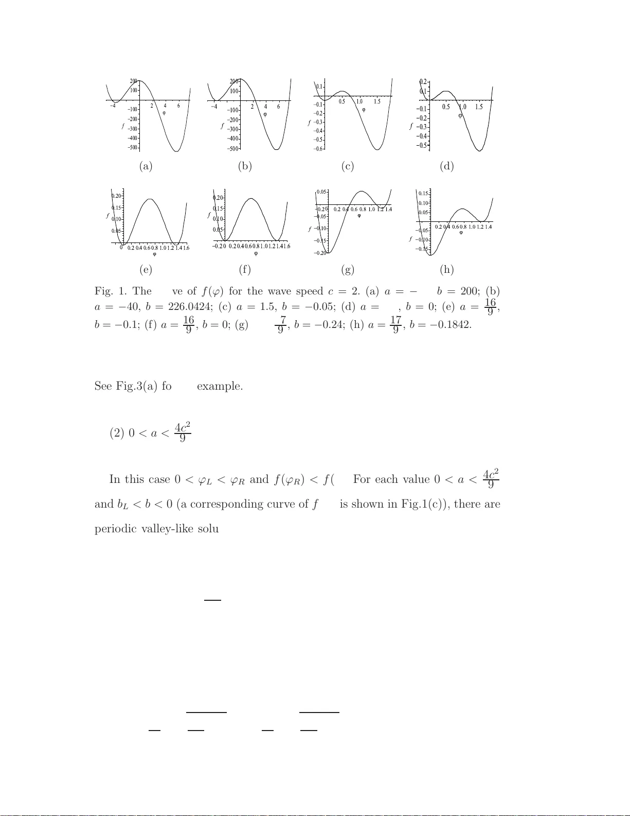
Soliton and p erio di c w a v e solutions t o the osmosis K(2, 2) equation Jiangb o Zhou ∗ , Lixin Tia n , Xinghua F an Nonline ar Scientific R ese ar ch Center, F aculty of Scienc e, Jiangsu Univ ersity, Zhenjiang, Jiangsu 212013, China Abstract In this pap er, t w o typ es o f trav eling w a v e sol utions to the osmosis K(2, 2) equation u t + ( u 2 ) x − ( u 2 ) xxx = 0 are inv estigated. They are c haracterized b y tw o p arameters. The expresssions for the solito n and p erio dic wa ve s olutions are obtained. Key wor ds: osmosis K (2, 2) equation, solito n, p er io dic w av e solution 1991 MSC: 35G25, 3 5G30, 35L05 1 In tro duction In 1 993, Rosenau and Hyman [ 1 ] in tro duced a gen uinely nonlinear disp er- siv e equation, a sp ecial ty p e of K dV equation, of the form u t + a ( u n ) x + ( u n ) xxx = 0 , n > 1 , (1.1) ∗ Corresp onding author. Email addr ess: zho ujiangbo@yaho o.cn (Jiangb o Zhou ). Preprint subm itte d to 12 No v ember 2018 where a is a constan t and b oth the con v ection term ( u n ) x and the disp er- sion effect term ( u n ) xxx are nonlinear. These equations arise in the pro cess of understanding the role of nonlinear disp ersion in the formation of structures lik e liquid drops. Rosenau and Hy man deriv ed solutions called compactons to Eq.( 1.1 ) and sho w ed that while compactons are the essence o f the fo cusing branc h where a > 0, spik es, p eaks, and cusps are the hallmark of the de fo cus- ing branc h where a < 0 whic h also supp orts the motion of kink s. F urther, the negativ e branc h, where a < 0, w as found to g iv e r ise to solita ry patterns having cusps or infinite slopes. Th e focusing branc h and the defocusing branc h repre - sen t t w o differen t mo dels , eac h leading to a different ph ysical struc ture. Man y p o w erful metho ds w ere applied to construct the exact solutions to Eq.( 1.1 ), suc h as Adomain metho d [ 2 ], homotopy p erturbation metho d [ 3 ], Exp-function metho d [ 4 ], v aria tional iteratio n metho d [ 5 ], v ar ia tional metho d [ 6 , 7 ]. In [ 8 ], W azw az studied a generalized forms of the Eq.( 1.1 ), that is mK ( n, n ) equa- tions and defined by u n − 1 u t + a ( u n ) x + b ( u n ) xxx = 0 , n > 1 , (1.2) where a, b are constants. He sho w ed how to construct compact and noncompact solutions to Eq.( 1.2 ) and discussed it in hig her dimensional spaces in [ 9 ]. Chen et al. [ 10 ] sho w ed ho w to construct the general solutions a nd some sp ecial exact solutions to Eq.( 1.2 ) in higher dimensional spatial domains. He et al. [ 11 ] considered the bifurcatio n b eha vior o f tra ve lling wa v e solutions to Eq.( 1.2 ). Under different parametric conditions, smo oth and non-smoo th p erio dic w av e solutions, solita r y wa ve solutions and kink and an ti-kink wa v e solutions were obtained. Y an [ 12 ] further extended Eq.( 1.2 ) t o b e a more general form u m − 1 u t + a ( u n ) x + b ( u k ) xxx = 0 , nk 6 = 1 , (1.3) 2 And using some direct ansatze, some abundan t new compacton solutions, solitary w a ve solutions and p erio dic w a v e solutions to Eq .( 1.3 ) w ere obtained. By using some transformations, Y an [ 13 ] obtained some Jacobi elliptic function solutions to Eq.( 1.3 ). Bisw as [ 14 ] obtained 1-soliton solution of equation with the generalized ev olution term ( u l ) t + a ( u m ) u x + b ( u n ) xxx = 0 , (1.4) where a, b ar e constan ts, while l , m and n are p ositiv e integers. Zh u et al. [ 15 ] applied the decomp osition metho d a nd sym b olic computation system to dev elop some new exact solitary w a v e solutions to the K (2 , 2 , 1) eq uation u t + ( u 2 ) x − ( u 2 ) xxx + u xxxxx = 0 , (1.5) and the K (3 , 3 , 1) equ ation u t + ( u 3 ) x − ( u 3 ) xxx + u xxxxx = 0 . (1.6) Recen t ly , Xu and Tian [ 16 ] in tro duced the osmosis K (2 , 2) equation u t + ( u 2 ) x − ( u 2 ) xxx = 0 , (1.7) w ere the p ositiv e con v ection term ( u 2 ) x means the conv ection mov es along the motion direction, a nd the negativ e disp ersiv e term ( u 2 ) xxx denotes the con tracting disp ersion. They obt a ined the p eak ed solitary w av e solution and the p erio dic cusp wa ve solution to Eq.( 1.7 ). In [ 17 ], the authors o bta ined the smo oth soliton solutio ns to Eq.( 1.7 ). In this pap er, following V akhnenk o and P ark es’s strategy [ 18 , 19 ] w e con tin ue to inv estigate the tra v eling w av e solutions to Eq.( 1.7 ) and obtain solito n and p erio dic w a v e solutions. O ur work in this pap er cov ers and extends the results in [ 16 , 17 ] a nd ma y help p eople to kno w 3 deeply t he described ph ysical pro ces s and possible applications of the osmosis K(2, 2) equation. The remainder of this pap er is o r g anized as follo ws. In Section 2, for com- pleteness and readabilit y , w e rep eat App endix A in [ 19 ], whic h discuss the solutions to a first-order ordinary differen tial equaion. In Section 3, w e show that, for trav elng wa ve solutions, Eq.( 1.7 ) may b e reduced to a first-order ordinary differen tial equation inv olving t w o arbitrary inte grat io n constants a and b . W e sho w that there are four distinct p erio dic solutions correspo nding to four different ranges of v alues of a and restricted ranges of v a lues of b . A short conclusion is give n in Section 4. 2 Solutions to a first-order ordinary differential equaion This s ection is due to V akhnenk o and Park es (see App endix A in [ 19 ]). F or completeness and readabilit y , w e state it in the f ollo wing. Consider solutions to the follow ing ordinary differential equation ( ϕϕ ξ ) 2 = ε 2 f ( ϕ ) , (2.1) where f ( ϕ ) = ( ϕ − ϕ 1 )( ϕ − ϕ 2 )( ϕ 3 − ϕ )( ϕ 4 − ϕ ) , (2.2) and ϕ 1 , ϕ 2 , ϕ 3 , ϕ 4 are ch osen to b e real constan ts with ϕ 1 ≤ ϕ 2 ≤ ϕ ≤ ϕ 3 ≤ ϕ 4 . 4 F ollow ing [ 20 ] w e introduce ζ defined b y dξ dζ = ϕ ε , (2.3) so that Eq.( 2.1 ) b ecomes ( ϕ ζ ) 2 = f ( ϕ ) . (2.4) Eq.( 2.4 ) has tw o p ossible forms o f solutio n. The first form is found using result 25 4.00 in [ 21 ]. Its para metric for m is                ϕ = ϕ 2 − ϕ 1 n sn 2 ( w | m ) 1 − n sn 2 ( w | m ) , ξ = 1 εp ( w ϕ 1 + ( ϕ 2 − ϕ 1 )Π( n ; w | m )) , (2.5) with w as the pa rameter, where m = ( ϕ 3 − ϕ 2 )( ϕ 4 − ϕ 1 ) ( ϕ 4 − ϕ 2 )( ϕ 3 − ϕ 1 ) , p = 1 2 q ( ϕ 4 − ϕ 2 )( ϕ 3 − ϕ 1 ) , w = pζ , (2.6) and n = ϕ 3 − ϕ 2 ϕ 3 − ϕ 1 . (2.7) In ( 2.5 ) sn( w | m ) is a Jacobian elliptic function, where the notation is as use d in Chapter 16 of [ 22 ]. Π( n ; w | m ) is the elliptic integral of the third kind and the notation is as used in Section 17.2.15 of [ 22 ]. The solution to Eq.( 2.1 ) is given in pa r a metric form by ( 2.5 ) with w as the parameter. With resp ect to w , ϕ in ( 2.5 ) is p erio dic with p erio d 2 K ( m ), where K ( m ) is the complete elliptic integral of the first kind. It follows from 5 ( 2.5 ) that the w av elength λ of the solution to ( 2 .1 ) is λ = 2 εp | ϕ 1 K ( m ) + ( ϕ 2 − ϕ 1 )Π( n | m ) | . (2.8) where Π( n | m ) is the complete elliptic integral of the third kind. When ϕ 3 = ϕ 4 , m = 1, ( 2.5 ) b ecomes                ϕ = ϕ 2 − ϕ 1 n tanh 2 w 1 − n tanh 2 w , ξ = 1 ε ( w ϕ 3 p − 2 tanh − 1 ( √ n tanh w )) . (2.9) The second form of t he solution to Eq.( 2.4 ) is found using result 25 5 .00 in [ 21 ]. Its parametric fo r m is                ϕ = ϕ 3 − ϕ 4 n sn 2 ( w | m ) 1 − n sn 2 ( w | m ) , ξ = 1 εp ( w ϕ 4 − ( ϕ 4 − ϕ 3 )Π( n ; w | m )) , (2.10) where m, p, w are as in ( 2.6 ), and n = ϕ 3 − ϕ 2 ϕ 4 − ϕ 2 . (2.11) The solution to Eq.( 2.1 ) is giv en in pa r ametric form by ( 2.10 ) with w as the parameter. The wa v elength λ of the solution to ( 2.1 ) is λ = 2 εp | ϕ 4 K ( m ) − ( ϕ 4 − ϕ 3 )Π( n | m ) | . (2.12) 6 When ϕ 1 = ϕ 2 , m = 1, ( 2.10 ) b ecomes                ϕ = ϕ 3 − ϕ 4 n tanh 2 w 1 − n tanh 2 w , ξ = 1 ε ( w ϕ 2 p + 2 tanh − 1 ( √ n tanh w )) . (2.13) 3 Solitary and p erio dic wa ve solutions to E q.( 1.7 ) Eq.( 1.7 ) can also b e written in the form u t + 2 u u x − 6 u x u xx − 2 uu xxx = 0 . (3.1) Let u = ϕ ( ξ ) + c with ξ = x − ct be a tra velin g w av e solution to Eq.( 3.1 ), t hen it follows that − cϕ ξ + 2 ϕ ϕ ξ − 6 ϕ ξ ϕ ξ ξ − 2 ϕϕ ξ ξ ξ = 0 , (3.2) where ϕ ξ is the deriv a t ive of function ϕ with resp ect to ξ . In tegrating ( 3.2 ) twic e with resp ect to ξ yields ( ϕϕ ξ ) 2 = 1 4 ( ϕ 4 − 4 c 3 ϕ 3 + aϕ 2 + b ) , (3.3) where a and b are t w o arbitrary in tegration constan ts. Eq.( 3.3 ) is in the f o rm of Eq.( 2.1 ) with ε = 1 2 and f ( ϕ ) = ( ϕ 4 − 4 c 3 ϕ 3 + aϕ 2 + b ). F or conv enience w e define g ( ϕ ) and h ( ϕ ) b y f ( ϕ ) = ϕ 2 g ( ϕ ) + b, where g ( ϕ ) = ϕ 2 − 4 c 3 ϕ + a, (3.4) f ′ ( ϕ ) = 2 ϕh ( ϕ ) , where h ( ϕ ) = 2 ϕ 2 − 2 cϕ + a, (3.5) 7 and define ϕ L , ϕ R , b L , and b R b y ϕ L = 1 2 ( c − √ c 2 − 2 a ) , ϕ R = 1 2 ( c + √ c 2 − 2 a ) , (3.6) b L = − ϕ 2 L g ( ϕ L ) = a 2 4 − 1 2 c 2 a + c 4 6 − 1 6 ( c 3 − 2 ac ) √ c 2 − 2 a, (3.7) b R = − ϕ 2 L g ( ϕ L ) = a 2 4 − 1 2 c 2 a + c 4 6 + 1 6 ( c 3 − 2 ac ) √ c 2 − 2 a. (3.8) Ob viously , ϕ L , ϕ R are the ro ots of h ( ϕ ) = 0. Without loss of generalit y , w e supp ose the w av e sp eed c > 0. In the fol- lo wing, supp ose that a < c 2 2 and a 6 = 0 for eac h v alue c > 0, suc h that f ( ϕ ) has three distinct stationary p oin ts: ϕ L , ϕ R , 0 and comprise t w o minim ums separated b y a maximum. Under this assumption, Eq.( 1.7 ) has p eriodic and solitary w av e solutions that ha v e differen t a nalytical fo rms dep ending on the v alues o f a and b as follow s: (1) a < 0 In this case ϕ L < 0 < ϕ R and f ( ϕ L ) > f ( ϕ R ). F or eac h v alue a < 0 and 0 < b < b L (a corresp onding curv e of f ( ϕ ) is sho wn in Fig.1(a)), there are p erio dic lo op-lik e solutions to Eq.( 3.3 ) giv en b y ( 2.10 ) so that 0 < m < 1, and with w av elength give n by ( 2.12 ). See Fig.2(a) for an example. The case a < 0 and b = b L (a corresp onding curv e of f ( ϕ ) is sho wn in Fig.1(b)) corresp onds to the limit ϕ 1 = ϕ 2 = ϕ L so that m = 1, and t hen the solution is a lo op-lik e solita ry w a v e give n by ( 2.13 ) with ϕ 2 ≤ ϕ < ϕ R and ϕ 3 = 1 2 √ c 2 − 2 a + c 6 − 1 3 q c 2 + 3 c √ 4 − 2 a, (3.9) ϕ 4 = 1 2 √ c 2 − 2 a + c 6 + 1 3 q c 2 + 3 c √ 4 − 2 a. (3.10) 8 4 K 4 2 4 6 f K 500 K 400 K 300 K 200 K 100 100 200 (a) 4 K 4 2 4 6 f K 500 K 400 K 300 K 200 K 100 100 200 (b) 4 0.5 1.0 1.5 f K 0.6 K 0.5 K 0.4 K 0.3 K 0.2 K 0.1 0.1 (c) 4 0.5 1.0 1.5 f K 0.5 K 0.4 K 0.3 K 0.2 K 0.1 0.1 0.2 (d) 4 0 0.2 0.4 0.6 0.8 1.0 1.2 1.4 1.6 f 0.05 0.10 0.15 0.20 (e) 4 K 0.2 0 0.2 0.4 0.6 0.8 1.0 1.2 1.4 1.6 f 0.05 0.10 0.15 0.20 (f ) 4 K 0.2 0 0.2 0.4 0.6 0.8 1.0 1.2 1.4 f K 0.20 K 0.15 K 0.10 K 0.05 0.05 (g) 4 0.2 0.4 0.6 0.8 1.0 1.2 1.4 f K 0.15 K 0.10 K 0.05 0.05 0.10 0.15 (h) Fig. 1. Th e cur v e of f ( ϕ ) for the wa ve sp eed c = 2. (a) a = − 40, b = 200; (b) a = − 40, b = 226 . 0424 ; (c) a = 1 . 5, b = − 0 . 05; (d) a = 1 . 5, b = 0; (e) a = 16 9 , b = − 0 . 1; (f ) a = 16 9 , b = 0; (g) a = 17 9 , b = − 0 . 24; (h) a = 17 9 , b = − 0 . 1842. See Fig.3(a) for an example. (2) 0 < a < 4 c 2 9 In this case 0 < ϕ L < ϕ R and f ( ϕ R ) < f (0) . F or eac h v alue 0 < a < 4 c 2 9 and b L < b < 0 (a cor r esp onding c urve of f ( ϕ ) is sho wn in F ig.1(c)), there are p erio dic v alley-lik e solutions to Eq.( 3.3 ) g iven by ( 2.1 0 ) so that 0 < m < 1, and with w a v elength given b y ( 2.12 ). See Fig .2(b) for an example. The case 0 < a < 4 c 2 9 and b = 0 (a corr esp onding curv e of f ( ϕ ) is sho wn in Fig.1(d)) corresp onds to the limit ϕ 1 = ϕ 2 = 0 so that m = 1, and then the solution can be give n b y ( 2.13 ) with ϕ 3 and ϕ 4 giv en by the ro ots of g ( ϕ ) = 0, namely ϕ 3 = 2 c 3 − s 4 c 2 9 − a, ϕ 4 = 2 c 3 + s 4 c 2 9 − a. (3.11) 9 In this case w e obtain a w eak solution, namely the p erio dic do wn w ard- cusp w a v e ϕ = ϕ ( ξ − 2 j ξ m ) , (2 j − 1) ξ m < ξ < (2 j + 1) ξ m , j = 0 , ± 1 , ± 2 , · · · , (3.12) where ϕ ( ξ ) = ( ϕ 3 − ϕ 4 tanh 2 ( ξ / 4)) cosh 2 ( ξ / 4) , (3.13) and ξ m = 4 tanh − 1 s ϕ 3 ϕ 4 . (3.14) See Fig.3(b) fo r an example. x K 10 K 5 0 5 10 4 0.5 1.0 1.5 2.0 (a) x K 10 K 5 0 5 10 4 0.3 0.4 0.5 0.6 0.7 (b) x K 10 K 5 0 5 10 4 0.4 0.6 0.8 1.0 (c) x K 20 K 10 0 10 20 4 0.6 0.7 0.8 0.9 1.0 1.1 (d) Fig. 2. Pe rio dic solutions to Eq.( 3.3 ) with 0 < m < 1 and the wa ve sp eed c = 2. (a) a = − 40, b = 200 so m = 0 . 8978; (b) a = 1 . 5, b = − 0 . 05 so m = 0 . 6893 ; (c) a = 16 9 , b = − 0 . 1 so m = 0 . 8254; (d) a = 17 9 , b = − 0 . 24 so m = 0 . 8412. (3) a = 4 c 2 9 In this case 0 < ϕ L < ϕ R and f ( ϕ R ) = f (0). F or a = 4 c 2 9 and eac h v alue b L < b < 0 (a corresp onding curv e of f ( ϕ ) is shown in Fig.1(e)), there are 10 x K 4 K 2 2 4 4 K 3 K 2 K 1 1 2 (a) x K 8 K 6 K 4 K 2 0 2 4 6 8 4 0.1 0.3 0.5 0.8 (b) x K 10 K 5 0 5 10 4 0.2 0.4 0.6 0.8 1.0 1.2 (c) x K 10 K 5 0 5 10 4 0.6 0.8 1.0 1.2 (d) Fig. 3. Solutions to Eq.( 3.3 ) with m = 1 and the wa ve sp eed c = 2. (a) a = − 40, b = 226 . 0 424; (b ) a = 1 . 5, b = 0; (c) a = 16 9 , b = 0; (d) a = 17 9 , b = − 0 . 1842. p erio dic v alley-lik e solutions to Eq.( 3.3 ) giv en b y ( 2.5 ) so tha t 0 < m < 1, and with w a v elength given b y ( 2.8 ). See Fig.2(c) for an example. The case a = 4 c 2 9 and b = 0 (a corresp onding curve of f ( ϕ ) is sho wn in Fig.1(f )) cor r esp onds to the limit ϕ 3 = ϕ 4 = ϕ R = 2 c 3 and ϕ 1 = ϕ 2 = 0 so that m = 1. In this case neither ( 2.9 ) nor ( 2.1 3 ) is appropriate. Instead we consider Eq.( 3.3 ) with f ( ϕ ) = 1 4 ϕ 2 ( ϕ − 2 c 3 ) 2 and note that the b ound solution has 0 < ϕ < 2 c 3 . On integrating Eq.( 3.3 ) a nd setting ϕ = 0 at ξ = 0 w e obtain a w eak solution ϕ = − 2 c 3 exp ( − 1 2 | ξ | ) + 2 c 3 , (3.15) i.e. a sin gle v a lley-lik e p eak ed solution with amplitude 2 c 3 . See Fig.3(c) fo r an example. (4) 4 c 2 9 < a < c 2 2 11 In t his case 0 < ϕ L < ϕ R and f ( ϕ R ) > f (0). F o r eac h v alue 4 c 2 9 < a < c 2 2 and b L < b < b R (a corresp onding curv e of f ( ϕ ) is show n in Fig .1(g)), there are p erio dic v alley-lik e solutions to Eq.( 3.3 ) g iv en b y ( 2.5 ) so that 0 < m < 1 , and with w a v elength given b y ( 2.8 ). See Fig.2(d) fo r an example. The case 4 c 2 9 < a < c 2 2 and b = b R (a corresp onding curv e of f ( ϕ ) is s hown in Fig.1(h) ) corresp onds to the limit ϕ 3 = ϕ 4 = ϕ R so that m = 1, and then the solution is a v elley-lik e solitary wa ve giv en b y ( 2.10 ) with ϕ L < ϕ ≤ ϕ 3 and ϕ 1 = c 6 − 1 2 √ c 2 − 2 a − 1 3 q c 2 − 3 c √ c 2 − 2 a, (3.16) ϕ 2 = c 6 − 1 2 √ c 2 − 2 a + 1 3 q c 2 − 3 c √ c 2 − 2 a. ( 3 .17) See Fig.3(d) fo r an example. 4 Conclusion In t his pap er, w e hav e found expressions for t w o types of t r a veling wa v e solutions to the osmosis K (2, 2) equation, that is, the soliton and p erio dic w a v e solutions. These solutions depend, in effect, on tw o pa r a meters a a nd m . F or m = 1, there are lo op-lik e ( a < 0), p eak on ( a = 4 c 2 9 ) and smo oth ( 4 c 2 9 < a < c 2 2 ) soliton solutions. F or m = 1 , 0 < a < 4 c 2 9 or 0 < m < 1 , a < c 2 2 and a 6 = 0, there are p erio dic w av e solutions. 12 References [1] P . Rosenau, J. M. Hyman, Compactons: solitons with finite wa ve lengths, Ph ys. Rev. Lett. 7 0 (1993) 564 -567. [2] A. M. W azw az, Compactons and solitary patterns structur es for v arian ts of the KdV and th e KP equatio ns, Ap pl. Math. Comput. 138 (2003) 309-3 19. [3] J. H. He, Homotop y p ertur b atio n m ethod f or bifurcation of nonlinear p r oblems, In t. J Nonlinea r Sci. Numer. Sim ulat. 6 (2005) 207- 208. [4] J. H. He, X. H. W u, Exp-fun ctio n metho d for nonlinear wa v e equations, Chaos, Solitons and F r act als 30 (2006) 700 -708. [5] J. H. He, X. H. W u, Construction of solitary solution and compacto n-like solution by v ariational iteratio n metho d, Chaos, Solitons and F ractals 29 (2006) 108-1 13. [6] J. H. He, Some asymp tot ic metho ds for strongly nonlinear equations, Int. J Mo dern Ph ys. B 20 (2006) 1141-1 199. [7] L. Xu, V ariational ap p roac h to solitons of nonlinear disp ers iv e equations, Ch ao s, Solitons and F r act als 37 (2008) 137 -143. [8] A. M. W azw az, General compacts s olit ary patterns solutions for mo dified nonlinear disp ersive equation in higher dimensional spaces, Math. Compu t. Sim ulat. 59 (200 2) 519-531. [9] A. M. W azw az, C ompact and n oncompact structures for a v arian t of KdV equation in higher dimens ions , Appl. Mat h. Compu t. 132 (2 002) 29-45. [10] Y. Chen, B. Li, H. Q. Zh ang, New exact solutions for mo dified nonlinear disp ersiv e equations in higher d imensions sp aces, Math. Comput. Sim ul. 64 (2004 ) 549-55 9. 13 [11] B. He, Q. Me ng, W. Rui, Y. Long, Bifurcations of tr a ve lling wa v e solutions for the equation, Commun. No nlinear Sci. Numer. Sim u lat. 13 (2008 ) 2114-2123. [12] Z . Y. Y an, Mo dified nonlinearly disp ersive mK ( m, n, k ) equations: I. New compacton solutions and solitary pattern solutions, Comput. Ph ys. Commun. 152 (20 03) 25-33. [13] Z . Y. Y an, Mo d ified nonlinearly disp ersiv e equ ations: I I. Jacobi elliptic fu n ctio n solutions, Comput. P h ys. Comm un . 153 (2003 ) 1-16. [14] A. Biswas, 1-solit on solution of the equation with generalized ev olution, Phys. Lett. A 372 (2008) 460 1-4602. [15] Y. G. Zhu, K. T on g, T. C. Lu, New exact solitary-w a ve solutions for the K (2 , 2 , 1) and K (3 , 3 , 1) equations, Chaos, S olito ns and F ractals 33 (2007) 1411- 1416. [16] C . H. Xu, L. X. T ian, Th e bifur cat ion an d p eak on for K (2 , 2) equation w ith osmosis disp ersion, Chaos, Solitons and F r act als 40 (200 9) 893-901. [17] J . B. Zhou, L. X. Tian, Soliton solution of the osmosis K(2, 2) equati on, Phys. Lett. A 372 (2008) 623 2-6234. [18] V. O. V akhnenko, E. J. P ark es, Explicit solutions of the Camassa-Ho lm equation, Chaos, S olit ons and F r act als 26 (2005) 130 9-1316. [19] V. O. V akhnenko, E. J. P ark es, P erio dic and solitary-w a v e solutions of the Degasp er is-Pr ocesi equation, Chaos, Solitons and F r act als 20 (2004) 1059- 1073. [20] E. J. P arke s, Th e stability of solutions of V akhn enk o’s equation, J . Ph ys. A Math. Gen. 26 (1993) 64 69-75. [21] P . F. Byrd, M. D. F riedm an , Hand b ook of elliptic in tegrals for engineers and scien tists, Springer, Berlin, 19 71. [22] M. Abr amo witz, I. A. Stegun, Handb o ok of mathematical functions, Dov er Publications, New Y ork, 197 2. 14