Worst case attacks against binary probabilistic traitor tracing codes

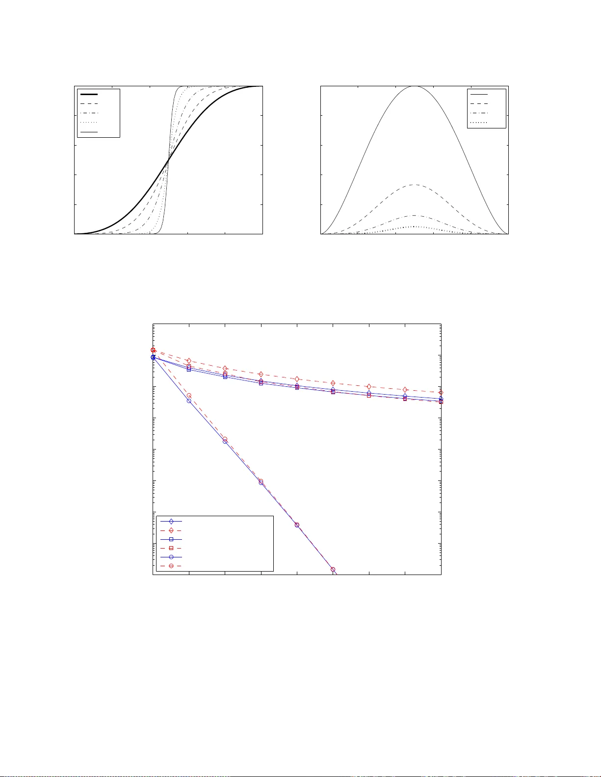
1 W orst case att acks against binary probabilistic traitor traci ng codes T eddy Furon and Luis P ´ erez-Freire Abstract An insightful vie w into the design of traitor tracing codes should necessarily consider t he worst case att acks that the colluders can lead. This paper takes an information-theoretic point of view where the worst case attack is defined as the collusion strate gy minimizing the achiev able rate of the trait or tracing code. T wo different decoders are en visaged , the joint decoder and the simple decoder , as recently defined by P . M oulin [1]. Sev eral classes of colluders are defined with increasing po wer . The worst case attack is deriv ed for each class and each decoder when applied to T ardos’ codes and a probabilistic version of the Boneh -Shaw construction. T his contextual study gi ves the real rates achie v able by the binary probabilistic traitor tracing codes. Attacks usually considered in literature, such as majority or minority votes, are indeed largely suboptimal. T his article also shows the utmost importance of the time-sharing concept in probabilistic codes. I . I NT RO D U C T I O N This article deals with traitor tr acing which is also known as acti ve fingerp rinting, co ntent serializatio n, user foren sics or transactional watermarking . A typical applicatio n is, for instance , as follows: A video on de mand server distributes personal copies of the same co ntent to n buyers. Some are dishone st users whose goal is to illegally redistribute a pirate copy . The rights ho lder is intere sted in iden tifying these d ishonest users. For th is pu rpose, a un ique user identifier consisting o n a sequence of m symbo ls is embed ded in each video co ntent thanks to a watermarking techniq ue, thu s producing n different (althoug h perceptu ally similar) copies. This allows tracing back wh ich user has illegally redistributed his copy . However , there might be a co llusion of c disho nest users, c > 1 . This collusion mixes their copies in order to f orge a pirated content which contains none of the identifiers b ut a mixture of them. The traitor tracin g code inv ented by Gab or T ardos in 2003 [2] beco mes more an d m ore popu lar . Th is cod e is a pr obabilistic weak traito r tr acing co de, wh ere the probab ility of accusing an innocent is not null. Its perform ance is usually ev aluated in terms of th e prob ability P F A of accusing an in nocent and the probab ility of missing all collud ers P F N . Most of the articles dealing with the T ardos code aim at findin g a tighte r lower bound on the len gth of the co de. In his seminal work, G. T ardos shows that, in ord er to guaran tee P F A < ǫ 1 and P F N < ǫ c/ 4 1 as defined in th e Boneh & Shaw prob lem [ 3], the code length must satisfy m > 100 c 2 log n/ǫ 1 . Many resear chers f ound th e constant 100 too ar bitrary . Better approxima tions 1 are 4 π 2 [4], 8 5 [5], and 1 6 [6]. A main improvement came from the symmetric d ecoding [7]. Other work s pr opose mor e practical implementatio ns of the T ardos code [8]. The reader will a lso find a pedagogic al presentatio n o f this code in [9]. Our ar ticle is very different than these past threads of studies a s we give the theo retical p erform ances of the code whatev er the accusation algorith m. In a nutshell, our work consists in app lying the results of [1]. In this article , P . Moulin gives the definition of cap acity for the tr aitor tracing pr oblem, providing exact cap acity expressions for the blind model, i.e. when the decoder doe s not know in advance neith er the numb er of collud ers nor the particular c ollusion strategy followed by them . So far , only bound s to the capacity had been deri ved by oth er au thors (see references in [ 1]). In w ords, capacity is defined as the m aximum (over all traitor tracing co des) of the minimum (over all strategies allowed b y the c ollusion mod el) o f an app ropriate mutual information func tional. Nevertheless, the p roblems of finding the best traitor tracing codes and the optimal collusion attacks are left op en, alth ough some important h ints are given in [1] and more recently in [10]. Ou r results are not in the direction of solvin g this g ame-theo retic problem. W e consid er specific binary fingerp rinting co des and seek for the collusion strategy minim izing the mutual info rmation. Ther efore, we can not speak of capacity o f a giv en collusion channel as in [1], but of the maximu m ach iev able rate of a given binary cod e. Our re sults are mainly aimed at pr oviding more insigh t into the binar y T ardos code, but the methodolo gy can b e easily extended, in general, to other cod e con structions based on the sam e p rinciples. I n fact, as explain ed in the sequel, our study also dea ls with a pr obabilistic version of the Boneh & Shaw code [3] . The g oal of o ur stud y is twofold. First, it seems that an inv ariance proper ty governs the design o f T ardos cod e [9]: the Markov lower bo unds on code length d erived in [2 ], [4], [5] inv olve m eans and variances of the inno cents and co lluders scores which are inv ariant with respect to the co llusion strategy . Theref ore, this nuisance parameter un known at the accusatio n side is no longer a problem since the bounds hold whate ver its value. A priori, there is no co llusion attack which is worse 1 Numbers are gi ven for the non symmetric decoding, where symbols ‘0’ are discarded as in the original T ardos setup. 2 than any othe rs. This is yet only true as far as the first and second o rder statistics of the scores are concer ned. Higher ord er statistics do not share this inv ariance prop erty . Fu rthermo re, this in variance property o nly hold s for the deco der o riginally suggested by G. T ardos. On co ntrary , the achiev able rate of the tra itor tracing cod e is an app ropriate measure to qu antify how d amageab le is a g iv en collusion process whatev er the decoding algorithm. Therefo re, we ar e lookin g f or the worst case collusion attack fo r a given numb er of co lluders m inimizing th is qu antity . T he cod e is dee med sound when ev er its rate is below this min imal m utual informatio n, hen ce the term m aximum achiev able rate. The se results clearly sh ow that classical assessment against, for instance, major ity o r minority attacks can largely ov erestimate the performan ce of the code because these are far f rom being the worst co llusion processes. The secon d goal of this article is to show the importan ce of time-sharing , which has been a lready high lighted in the theoretical deriv ations o f P . Mou lin [1], in practice when a b inary T ardos code is con sidered. Time-sharing is a concep t well known in mu ltiuser inf ormation theory [ 11], by which u sing two or mor e code s of different rates a n ew code can be constructed by using each code in disjoint fr actions of th e time. In the T ardos co de, the p robab ility of having a symbo l ‘1 ’ in a code sequence chan ges from o ne index i to another according to a given auxiliary r andom variable P , which is indeed the “time-sharing” v ariable th at selects the co de to be used in each index. T herefor e, th e achiev able rate of the codes studied in this paper is defined as an expecta tion o f a function over the time-sha ring random v ariable P . It is very interesting to plot this later f unction with respect to P . Some attacks succeed in can celing this f unction over a rang e. Theref ore, the suppor t and the values taken by the proba bility density functio n f ( P ) of the time-shar ing variable is of utmost impo rtance. An approp riate time-sharing leads to huge improvements, provided the time-sharin g sequence remains secret for the collu ders. Moreover , th is study also shows that even when this seque nce is disclosed, perfo rming traitor tracing is still possible in theory as the rate ne ver exactly can cels. An inte resting by prod uct of our analysis is that it indeed addresses the analysis of binary traitor tracing codes with out time-sharing, which has not been addressed before fr om the information -theoretic viewpoint, spec ially in th e case of the simple decoder . W e recently discovered that E. Amiri an d G. T ardo s [10], and ind epend ently Hu ang and Mo ulin [12], addr essed the same issues. Howe ver , relati vely few of their r esults cover exactly our propo sitions: • For the join t dec oder, they succeeded to derive in a game-th eoretic setting the capacity- achieving parameter f ( P ) . This is indeed a pr obability mass function (pm f - i.e. the time-sharin g variable is discrete) stro ngly de penden t on the collusion size. Howev er , in a real case scenario on e cannot for esee the exact numbe r of colluders: at most, a maximum collusion size can be anticipated . The code is guarantee d to perfor m well whenever the n umber of co lluders is below the predicted maximum ; ho wev er , fo r bigger collusion sizes the code bec omes unreliab le. Furthermor e, th e num erical computatio n o f the optimal f ( P ) seems not feasible fo r a large number of colluders [12]. This motiv ates th e interest in the study of th e pr obabilistic traitor trac ing cod e with a fixed con tinuous f ( P ) which, albeit sub optimal, do es reason ably well for any collusion size. Remarkably , the f ( P ) pro posed by T ardos which we study in this paper seems to be very close to the optimal f ( P ) when the numb er of colluders is very lar ge, acco rding to [12], and th e asym ptotic loss with respect to the capacity is only within a small factor . • For th e simple decoder, Amiri and T ardos [10] con sidered a scenario where all colluder identities were disclosed e xcept one, an d the d ecoder is loo king for the identity of th is unknown colluder . Our simp le decoder is the one defined by P . Moulin [1] which is very dif ferent and more realistic: no colluder is caught, and the goal of the decod er is to m ake a first accusation. Sec. II introdu ces all the mathema tical definition s and assumption s needed to derive the worst case a ttacks: th e type o f traitor tracing code we are dealin g with (Sec. II-B), the introduction of four different classes o f colluder s referred to as A, B, C and D ( Sec. II-C), and two possible ac cusation strategies b ased on the so-called join t and simple decoders (Sec. II-D). This p aper g iv es the worst case attacks tha t a giv en class of co lluders can lead a gainst a given family of d ecoders: joint decoder in Sec. III and simple d ecoder in Sec. IV. I I . M O D E L A. Notation First of all we summar ize the most important notational con ventions to b e used through out the p aper . Rando m v ariables and their realization s are d enoted by capital and lowercase letters, respectively . Boldface letter s deno te co lumn vector s. Calligraphic letters ar e re served for sets. Pr X [ x ] is the pro bability that the discrete rando m variable X takes the value x . The shorthand [ m ] will be used to d enote a sequence of indices { 1 , . . . , m } . H ( . ) deno tes entr opy of a discrete r andom variable. h b ( x ) = − x log ( x ) − (1 − x ) log (1 − x ) is th e b inary entro py . D K L ( Pr X || Pr Y ) is the Kullback -Leibler diver gence or relativ e entropy be tween the random variables X and Y . log , the logarithm to the base 2 , is preferab ly used in ord er to giv e all rates and entropies in bits, whereas ln is the natural logarithm. 3 B. B inary pr ob abilistic code wit h time-sharing W e briefly remind h ow the T ardos cod e is designed , as an examp le of a p robabilistic c ode with time -sharing. Th e b inary code X is composed of n seq uences of m bits. The seque nce X j = ( X ( j, 1) , · · · , X ( j, m )) T identifyin g u ser j is composed of m independen t binary symbols, with Pr X ( j,i ) [1] = p i , ∀ i ∈ [ m ] . The auxiliary rand om variables { P i } m i =1 are independent and iden tically distributed in the ran ge [0 , 1] acco rding to the probab ility density fun ction f ( p ) : P i ∼ f ( p ) . T ardos pd f f ( p ) =  π p p (1 − p )  − 1 is symmetric around 1 / 2 : f ( p ) = f (1 − p ) . It mean s that symbols ‘1’ a nd ‘0’ play a similar role with pr obability p or 1 − p . Both the code X and the time- sharing sequence p = ( p 1 , . . . , p m ) T must remain as secret parameters. In the original paper, the pdf is slightly different as it is defined in [ t, 1 − t ] where t > 0 is the cu t-off pa rameter fixed to 1 / 300 c . W e d o not consider this cut-off since the integrals are all well de fined over (0 , 1) . This d efinition mig ht en compass mo re finger printing codes than the T ardos one . Althoug h its con struction is very different, the Bon eh & Shaw cod e (BS) shares a similar statistical stru cture [3]. When n users are addressed, th e ratio P of symbol ‘1’ in the code symbo ls { X ( j, i ) } n j =1 for a given index i ∈ [ m ] can be considered as a discrete rand om v ariable whose prob ability mass functio n is given by Pr P [ k /n ] = 1 /n, ∀ k ∈ [ n ] . This m eans that the sequence identify ing user j is comp osed o f m binary sym bols, with Pr X ( j,i ) [1] = p i , ∀ i ∈ [ m ] , where p i ∈ { 1 / n , 2 /n, . . . , ( n − 1) /n , 1 } is ch osen e quipro bably . Therefo re, the resemblanc e with the T ardos con struction is clear: as n go es to in finity , this co de can b e constructed as a T ardos cod e but with a flat pdf over [0 , 1] : f ( p ) = 1 ∀ p ∈ [0 , 1] . Howe ver , the difference b etween the T ardos and the BS co des is that the rate of the latter is impo sed by construc tion. L et us define the rate R of a fin gerprin ting code by R = log ( n ) /m . In a BS co de, the r ate is known to be lo g( n ) /r ( n − 1) , where r is th e so-called “replication facto r” [3]. Howe ver , in ord er to per form a r eliable accusation, th e rate o f any code must be lower th an the cap acity of th e co llusion channel [1]. Finding the capacity in duced by a collusion process is a hard problem in ge neral. This paper on ly deals with the achiev able rate of T ardos-like co des (either with the T ardos pdf o r a flat p df to simulate a BS code), which is defined as the maximu m rate guaran teeing a r eliable decodin g for any collusion process in a gi ven c lass. C. Collusion pr ocess Denote the subset of collud er indices by C = { j 1 , · · · , j c } , and X C = { X j 1 , . . . , X j c } the restrictio n of the code to this subset. The c ollusion attack is th e pro cess of taking sequ ences in X C as inp uts and yieldin g the pirated seq uence Y as an output. T raitor tr acing cod es have b een first studied b y th e cryp tograp hic commun ity and a key-concept is the marking assumptio n introdu ced by Bo neh and Shaw [3]. It states that, in its n arrow-sense version , whatev er th e strategy of the collusion C , we have Y ( i ) ∈ { X ( j 1 , i ) , · · · , X ( j c , i ) } . In words, collud ers forge the pirated copy by assembling chunk s from their per sonal copies. It implies that if, at in dex i , the colluders’ symbols are identical, then this symb ol v alue is decoded at the i -th chu nk of the pirated copy . This is what waterma rkers have un derstood fro m the pioneerin g cryptog raphic work. Howe ver , this has led to miscon- ceptions. Another important thing is th e way cry ptograp hers have mo deled a host co ntent: it is a bin ary string where some symbols can be chang ed w ithout spoiling th e regular use of the co ntent. These loc ations ar e used to insert the co de seq uence symbols. Cryptograph ers assume tha t co lluders disclose codew ord sym bols from their identifying sequ ences comparing th eir personal copies symbol by sym bol. Th e colluders ca nnot spot a hidden sym bol if it is iden tical o n all copies, h ence the marking assumption. In a mu ltimedia application, for instance, th e content is typically divided into chunks. A chu nk can be a f ew second clip of audio or vid eo. Symbol X ( j, i ) is hidd en in the i -th chun k of the content with a watermark ing tech nique. This gi ves the i -th ch unk sent to th e j -th user . I n this p aper, we only ad dress collu sion processing wh ere the pira ted copy is fo rged by picking ch unks f rom th e colluders’ personal cop ies. W e do not cope with the mixing of several chu nks into one (we assume that the waterm arking technique is robust enoug h to handle this mixing collusion pr ocess). The marking assumption still h olds b ut for another re ason: as the co lluders ig nore the watermarking secret key , they cann ot create chunks of content watermarked with a symbol the y do not hav e. However , c ontrary to th e o riginal cryptograp hic model, this also implies that the colluders might not know which symbol is embedded in a chunk. 1) Mathem atical m odel: Our math ematical m odel of the collu sion is essentially ba sed on four m ain assum ptions. Th e first assumption is the m emoryle ss nature of the co llusion attack. Since the sy mbols of th e cod e are independent, it seems rele vant that the pirated sequen ce Y also sha res this property . Therefore, the value of Y ( i ) only depe nds o n { X ( j 1 , i ) , · · · , X ( j c , i ) } . The second assumption is the stationarity o f the collusion process. Excep t wh en the T ardos code is broken (this is explained in th e next section), we assume that the collusion strategy is in depend ent of the index i in the sequence. Ther efore, we can describe it forgetting th e index i in the sequel. The third assumption is that the colluders select the value o f the symbol Y 4 depend ing on the values of their symbols, but not on their order . That is, the collusion chann el is in variant to permutatio ns of { X ( j 1 , i ) , · · · , X ( j c , i ) } . Therefore, the input of the collusion process is ind eed the ty pe of th eir symbols. In th e binary case, this type is fu lly defined by the following sufficient statistic: the numb er Σ i of symbols ‘1’ : Σ i = P c j =1 X ( j, i ) . These three first assumptions greatly simp lify the an alysis of the pr oblem withou t restricting the power of the co lluders because they do no t pre vent them fro m implementing an o ptimal collusion attack (see sections 2 an d 3 of [1]). Hence, our approa ch does not im ply any loss o f generality . The fourth assump tion is that the collusion process ma y no t be deterministic, but ran dom. These fo ur assumptions yield that the collusion attack is f ully described by the f ollowing pa rameter vecto r: θ = ( θ 0 , . . . , θ c ) T , with θ σ = Pr Y [1 | Σ = σ ] . The fo llowing subsectio n gives examples of such co llusion attac ks, but we can already state that they all share the following prop erty: Th e marking assumption enforces that θ 0 = 0 a nd θ c = 1 . The authors of [10] also speak about ‘ eligible channel’. 2) Classes of collu ders: W e introdu ce f our classes of attacks with in creasing power . a) Class-A: The weakest kind of colluders decides the value of the symbol Y ( i ) without considering all th eir symbols. Before re ceiving the personal cop ies, these c dishonest users have alr eady agree d on how to forge the pira ted copy . This strategy amounts to set an assignation sequence ( M 1 , · · · , M m ) with M i ∈ C , such that Y ( i ) = X ( M i , i ) . W e a ssume that the colluders share th e risk, so that th e cardinality |{ i | M i = j } | ≈ m/ c , for all j ∈ C . The assigna tion sequence is random and indepen dent of the personal copies. Hence, for each collu sion size, Class-A has a sin gle collusion attack θ given by θ σ = σ / c , ∀ σ = 0 , . . . , c . For the sake of co herenc e with the subsequent n otation, we say that θ ∈ P A ( c ) , { c − 1 (0 , 1 , . . . , c − 1 , c ) T } . b) Class-B: This second class of colluder s differs fro m Class-A in the fact th at the assignatio n sequence is n ow a function o f th e p ersonal copies. Th ese co lluders ar e ab le to split their copies in chunk s and to co mpare them samp le by sample. Hence, for any index i , they are able to notice that, for instance, ch unks c j 1 i and c j 2 i are dif ferent o r identical. For binary em bedded symbols, they ca n constitute two stack s, each containing identical chunks. This allo ws ne w collusion processes such as majority v ote, minority v ote, coin flip [9]. The impor tant thing is that colluders can n otice differences between chun ks, but they canno t tell whic h chunk contain s symbol ‘ 0’. 2 Hence, symb ols ‘1’ an d ‘ 0’ play a sy mmetric ro le, wh ich strong ly lin ks the co ndition al prob abilities: Pr Y [1 | Σ = σ ] = Pr Y [0 | Σ = c − σ ] = 1 − Pr Y [1 | Σ = c − σ ] . There fore, Class-B collusion attacks are constrained in the following way: θ ∈ P B ( c ) , { θ : θ 0 = 0 , θ c = 1 , θ σ ∈ [0 , 1] fo r σ ∈ [ c − 1] , θ σ = 1 − θ c − σ , for σ ∈ [ c − 1] } . (1) Hence, a Class-B collusion attack has ⌊ ( c − 1) / 2 ⌋ degrees of freed om, and fo r ev en c we n ecessarily ha ve θ c/ 2 = 1 / 2 . Clearly , for c = 2 the only possible Cl ass-B collusion strategy is θ = { 0 , 0 . 5 , 1 } , wh ich is also the Class-A attack. Class-B collusion is rele vant fo r traitor tr acing in the multimed ia scen ario, wh ere each b it of the code is embed ded in a dif ferent chunk (fram e, group of fram es, etc.) of the multimedia signal b y means of a watermarking techn ique. The authors of [1 0] refer to this class as “strongly symmetric eligib le channel. ” c) Class-C: This is the classical collusion mo del u sed b y crypto graph ers sinc e Boneh and Shaw [ 3]. Th e bits are directly pasted in the ho st co ntent string, and thus the c olluders can compar e their co pies b itwise in order to d isclose th e location of the traitor tr acing code. Class-C collusio n attacks are no lon ger constrained like in Class B, an d new strategies are then possible such as the f ollowing: • All ‘1’ s. The colluders put the symbol ‘1’ whenever they can : θ σ = 1 , 0 < σ ≤ c , • All ‘0’ s. The colluders put the symbol ‘0’ whenever they can : θ σ = 0 , 0 ≤ σ < c , In general, a Class-C collusion strategy belon gs to th e following set: θ ∈ P C ( c ) , { θ : θ 0 = 0 , θ c = 1 , θ σ ∈ [0 , 1] , σ ∈ [ c ] } , (2) and therefor e it has c − 1 degrees of freedom . d) Class-D: This last class is quite spe cial because it no lon ger fulfills the stationarity assump tion introd uced in II-C1. No w , the k nowledge of the time-sharing sequence p is granted to the co lluders. Fr om a statis tical poin t of view , the condition al prob abilities d epend on Σ i and P i : Pr Y i [1 | Σ i , P i ] . The collusion mo del for this class is a set o f c + 1 fu nctions θ ( p ) = ( θ 0 ( p ) , . . . , θ c ( p )) T such that θ ( p ) ∈ P C ( c ) , ∀ p ∈ [0 , 1] , (3) The interest of Class-D is twofold: on one hand, it g iv es the rate achiev able by a code that d oes not perfo rm time-sharing (i.e. the value of p is fixed) an d on the other hand it shows the achiev able rate when the co de has been broken (i.e. the secret of the pro babilistic code has been disclosed), meanin g that the colluders know the value of p i for all index i ∈ [ m ] . Therefo re, th ey can adapt their strategy fo r each in dex chu nk according to its value p i . Notice that the attack is still assumed to be memoryless. 2 Note that in order this to be strict ly true, we need the probability distributio n of the time- sharing sequence to be symmetric, as it is the case in this paper . 5 D. Deco ding families The study of traitor tracing co des from an achievable rate stand point largely decou ples th eir per forman ces from a ny particular decoding algor ithm. Howev er , we consider two different families of decoder s: the simple decoder [1, Sec. 4] an d the joint decoder [1, Sec. 5]. The simple decod er c alculates the empirical mutual informatio n between each user cod ew ord and the p irated seque nce, wher eas the jo int d ecoder c alculates th e emp irical mutua l info rmation between each possible subset of c users and the pirated sequ ence. Due to their d ifferent nature, the two families have different achie vable rates. Briefly , the joint decod er rep resents what the accusation side cou ld do in an ide al world wh ere complexity is no t a matter , an d it has been sh own to be ca pacity-ach ieving. Howe ver , it has to tackle ( n c ) grou ps which seems h ardly affordable for large n . The simple decoder, suboptimal in general, represents the upper performance limit fo r more practical decoders. 1) Joint d ecoder: The a chiev able rate for th e joint deco der again st a given collusio n attack is based on the mu tual informa tion b etween Y , a symbol of the p irated sequence, an d X C , the symbols of the colluders’ code sequen ces [1, Sec. 5]. This h olds for any index thanks to th e symbol inde penden ce, and th is is taken in e xpectation over the time-shar ing ran dom variable P : R joint ( θ ) = 1 c E P [ I ( Y ; X C | P = p, Θ = θ )] = 1 c ( E P [ H ( Y | P = p, Θ = θ )] − E P [ H ( Y | X C , P = p, Θ = θ )]) = 1 c ( E P [ H ( Y | P = p, Θ = θ )] − E P [ H ( Y | Σ , P = p, Θ = θ )]) , (4) where Σ is the random variable defined as the number of ones in the set X C . Equality in (4) fo llows because of the assumption stated in Sec t. I I-C, namely that the outpu t of the collusion channe l only depen ds on the ty pe of X C , not on the ord er of its e lements. For the sake of clarity , we omit th e expression Θ = θ in the sequel, but all the probab ility , entropy or mutual informa tion expression s are given fo r a gi ven co llusion attack. Plugging the collusion m odel introduce d in II- C1, we h av e: Pr Y [1 | P = p ] = c X σ =0 θ σ Pr Σ [ σ | P = p ] , (5) Pr Y [1 | Σ = σ, P = p ] = θ σ , (6) with Pr Σ [ σ | P = p ] = ( c σ ) p σ (1 − p ) ( c − σ ) , known as the Bernstein polyno mials [13]. Therefo re, Eq . (4) can be r ewritten as: R joint ( θ ) = 1 c E P " h b c X σ =0 θ σ Pr Σ [ σ | P = p ] !# − c X σ =0 E P [ Pr Σ [ σ | P = p ]] h b ( θ σ ) ! . (7) A possible interp retation of (4) is th at the r ate can also be e xpressed in terms of the average discrim ination (or Kullback Leibler distance as [14]): R joint ( θ ) = E P [ D K L ( Pr Y , Σ || Pr Y Pr Σ | P = p )] /c, (8) = E P   X y ∈{ 0 , 1 } c X σ =0 Pr Σ [ σ | P = p ] Pr Y [ y | Σ = σ ] log  Pr Y [ y | Σ = σ ] Pr Y [ y | P = p ]    /c. (9) The usefulness of this expression will becom e p atent in Section III-B. 2) Simp le decoder: T he achiev able rate fo r the simple decoder against a given collusion attack is given in [1, Sec. 4]: R simple ( θ ) = E P [ I ( Y ; X | P = p )] = E P [ H ( Y | P = p )] − E P [ H ( Y | X , P = p )] (10) = E P [ D K L ( Pr X,Y || Pr X Pr Y | P = p )] (11) This links the notion of rate to th e inheren t cap ability of d istinguishing two hypothesis: • H 0 : User j is inn ocent, and his codew ord is in depend ent of Y gi ven P : Pr [ Y , X |H 0 ] = Pr [ Y ] Pr [ X ] , • H 1 : User j is gu ilty and Y ha s been created from his co dew ord: Pr [ Y , X |H 1 ] = Pr [ Y | X ] Pr [ X ] . The calculation of the rate needs the expr essions o f the conditiona l pr obabilities induced by the co llusion model: Pr Y [1 | X = 1 , P = p ] = c X k =1 θ k  c − 1 k − 1  p k − 1 (1 − p ) c − k , (12) Pr Y [1 | X = 0 , P = p ] = c − 1 X k =0 θ k  c − 1 k  p k (1 − p ) c − k − 1 . (13) 6 Pr o position 1: T wo simple considerations: • For the classes A, B and C, the following relationships h old: Pr Y [1 | X = 1 , P = p ] = Pr Y [1 | P = p ] + 1 − p c ∂ ∂ p Pr Y [1 | P = p ] , (14) Pr Y [1 | X = 0 , P = p ] = Pr Y [1 | P = p ] − p c ∂ ∂ p Pr Y [1 | P = p ] . (15) • For c = 2 , P A (2) = P B (2) . Pr o of: After some manipu lations, we have ∂ ∂ p Pr Y [1 | P = p ] = c ( Pr Y [1 | X = 1 , P = p ] − Pr Y [1 | X = 0 , P = p ]) . Moreover , Pr Y [1 | P = p ] = p Pr Y [1 | X = 1 , P = p ] + (1 − p ) Pr Y [1 | X = 0 , P = p ] . The second item is obvious. 3) Achievable r ate under Class-Z attack: For a gi ven d ecoding family an d size of collusion, the achiev able r ate of a code under Class- Z attack (with Z ∈ { A, B , C, D } ) is th e mutua l in formation pro duced b y the worst collu sion process in this class. For in stance, with straightforward notation: R Z simple ( c ) = min θ ∈P Z ( c ) R simple ( θ ) . (16) Since the collude rs are m ore and more powerful as we consider upcomin g classes , the following relationships hold for the simple decoder (and similarly for the jo int decode r): R D simple ( c ) ≤ R C simple ( c ) ≤ R B simple ( c ) ≤ R A simple ( c ) . (17) T o stre ss the importance of the time-sharing variable P , it is interesting to define the function r Z simple ( c, p 0 ) , I ( Y ; X | P = p 0 , Θ = θ ∗ ) , (18) where θ ∗ = ar g min θ ∈P Z ( c ) R simple ( θ ) . The strong non -conve xity of r Z simple ( c, p ) in p , in general, justifies the need of time -sharing [1], as will be seen. Obvio usly , R Z simple ( c ) = E P h r Z simple ( c, p ) i . The extension o f this definition to the joint decoder is straigh tforward. I I I . T H E J O I N T D E C O D E R A. Collu ders Class-A Pr o position 2: A Class-A c ollusion leads to pirated seq uence symbols whose pro bability is Pr Y [1 | P = p ] = p , fo r any collusion size. Hence, the achievable rates of the joint deco der ag ainst Class-A c ollusion is for the T ardos and the flat distribution: R A joint ( c ) = c − 1 E P [ h b ( P )] − c X σ =0 E P [ Pr Σ [ σ | P ]] h b ( σ /c ) ! . (19) Pr o of: Since we ha ve θ σ = σ / c , ∀ σ ∈ { 0 , . . . , c } , Pr Y [1 | P = p ] has a simple expression: Pr Y [1 | P = p ] = c − 1 E Σ [ σ | P = p ] = p. (20) The last equality comes fro m the fact that Σ is a random variable distributed as a binomial B ( c, p ) , so its expectation is cp . W ith the help of Ma thematica , th e e xpectation s find closed form expression s, and the achie vable rate in b its is for the T ard os pdf: R A joint ( c ) = c − 1 2 − log ( e ) − π − 1 c X σ =0 Γ( σ + 1 / 2)Γ( c − σ + 1 / 2 ) Γ( σ + 1)Γ( c − σ + 1) h b ( σ /c ) ! (21) whereas for the flat pdf (i.e. f or the proba bilistic BS code) : R A joint ( c ) = c − 1 log( e ) / 2 − ( c + 1 ) − 1 c X σ =0 h b ( σ /c ) . ! (22) The resulting achie vable rates are plotted in Fig . 1. These p lots suggest that they decrease as 1 /c 2 . This is confirmed by the next p roposition . 7 1 2 3 4 5 6 7 8 9 10 10 −5 10 −4 10 −3 10 −2 10 −1 10 0 c R joint (bits) Tardos, Class−A Probabilistic BS, Class−A Tardos, Class−B−C Probabilistic BS, Class−B−C Tardos, Class−D Probabilistic BS, Class−D Capacity, Class−B−C (Amiri & Tardos) Fig. 1. Achiev able rates for the joint decoder a gainst diffe rent c lasses of collusion, for T ardos and probabil istic BS code s. T he fingerprint ing ca pacity (accord ing to Amiri and T ardos) aga inst Class-B-C coll uders is plotted for compar ison. Pr o position 3: For any pdf f ( p ) : [0 , 1] → R + , we have (in natural units) lim c → + ∞ R A joint ( c ) − 1 2 ln(2) c 2 = 0 . (23) See Appendix A-A for the proof. Consider now the achievable rate as the expectation ov er P of the fu nction r A joint ( c, p ) defined accordin g to (18). This function , wh ich is p lotted in Fig. 2 for different values of c , is symmetr ic aro und p = 1 / 2 because h b ( σ /c ) = h b (( c − σ ) / c ) . For c = 2 and c = 3 , its ma ximum is in p = 1 / 2 . This sh ows th at the best pdf would be a Dirac’ s de lta in p = 1 / 2 . There would no longer be need for time-sharing variable P , and the code X would be comp osed of i.i. d. binary compon ents with Pr [ X j i = 1] = 1 / 2 . For c > 3 , the maximum is n o lon ger in p = 1 / 2 , but on two sym metric values depend ing o n c , so that th e ca pacity-ach ieving pdf is compo sed o f two Dirac’ s deltas. T his is a very special case whe re the capacity ca n b e numerically deri ved. Th e achie vable rates of the T a rdos and th e p robab ilistic BS co des ar e lower than the capacity , as can be seen in Fig . 1. T he next section sh ows ho wev er that the Dir ac’ s d elta pdf achie ving capacity in Class-A is a very da ngerou s choice under other collusion classes, and that time-sharing be comes a necessity . B. Collu ders Classes B a nd C 1) 2 c olluders: Thanks to Prop. 1, the ratio nale for Class-A also hold s for Class-B when c = 2 . T ardos code rate is R B joint (2) = 7 / 8 − log( e ) / 2 ≈ 0 . 154 bits, wher eas the rate fo r probab ilistic BS code ( i.e. flat p df) R B joint (2) = log( e ) / 4 − 1 / 6 ≈ 0 . 194 bits. The capacity is achieved with the Dirac’ s delta pdf, f ( p ) = δ ( p − 1 / 2) , and it is appro ximately 0 . 25 bits. W e found back th e same result as Amiri and T ardos (see lin e 2 of T able 1 in [10]). Howev er , this strategy is very risky if the number of colluders is actually b igger than 2 as we shall see in the n ext section. 2) More colluders: When c ≥ 3 , the analysis is much mo re complex and we hav e only succeeded to fin d out the worst collusion process and thus, the achie vable rate for a giv en p df f ( p ) . 8 0 0.2 0.4 0.6 0.8 1 10 −3 10 −2 10 −1 10 0 p c=2 c=3 c=5 c=10 P S f r a g r e p l a c e m e n t s r A joint ( c, p ) (bits) Fig. 2. Plot of r A joint ( c, p ) for the joint decoder unde r Class-A attack . W e resort now to th e expr ession (9) of the achiev able rate in terms of the relative entropy . The pr oblem of m inimizing (9) ca n be rewritten as a doub le minim ization, exactly like the Blahut-Ar imoto algo rithm f or th e co mputation of th e r ate- distortion function [14]. Th e m ain difference is th at o ur minimizatio n pr oblem cor respond s to a degener ate rate-distortio n problem where the only d istortion con straint is that θ ∈ P B − C ( c ) (in the sense th at θ ∈ P B ( c ) or θ ∈ P C ( c ) depend ing on the class o f colluders). The reade r is referred to [14] or [11, Chapt. 13] for a detailed presentatio n o f the Blahut-Ar imoto algorithm as we only e xplain its application to our model. In a slight abuse of notation, let us denote the rhs o f (9) by R ( Pr Y [ Y | P ] , θ ) . The worst collusio n pro cess is disclo sed by iterativ ely minim izing over each argument of this function, keeping the oth er con stant. T hus, each iteration is comprised of two steps: 1) In the first step of the k -th iter ation, for a fixed law Pr Y [1 | P = p ] = q ( k − 1) ( p ) wh ose expression complies with ( 5), we minim ize R ( q ( k − 1) ( p ) , θ ) over θ . Note that R ( q ( k − 1) ( p ) , θ ) is conve x in θ b ecause for fixed p 0 ∈ [0 , 1] , or equiv alently for fixed Pr Σ [ σ | P = p 0 ] , th e argument of the expec tation in (9) is conve x in θ [11, Th. 2.7.4 ], and the expectation o f this function over P is still con vex. Hence, the minimization of R ( q ( k − 1) ( p ) , θ ) amou nts to canceling the ( c − 1) partial derivati ves ( θ 0 and θ c are already fixed to 0 and 1, respectively). Notice that we also ha ve to imp ose the constraint θ ∈ P B − C ( c ) . Ignorin g tempo rarily this constraint, we ha ve ∂ ∂ θ σ R ( q ( k − 1) ( p ) , θ ) = 1 c E P  Pr Σ [ σ | P = p ]  log θ σ 1 − θ σ + log 1 − q ( k − 1) ( p ) q ( k − 1) ( p )  . (24) By setting the last expression to 0, we obtain θ ( k ) σ = 1 1 + B ( k ) ( σ ) , σ = 1 , . . . , c − 1 , (25) with B ( k ) ( σ ) = 2 ˆ   E P h Pr Σ [ σ | P = p ] log 1 − q ( k − 1) ( p ) q ( k − 1) ( p ) i E P [ Pr Σ [ σ | P = p ]]   . (26) Note that B ( k ) ( σ ) is well defined because: • q ( k − 1) ( p ) is a polynomial of degree c which equals 0 only for p = 0 ( resp. q ( k − 1) ( p ) = 1 o nly for p = 1 ) ; • Pr Σ [ σ | P = p ] is also a po lynom ial that goes to zero f or p = 0 and p = 1 . Hence, by continuity , th e n umerato r of (26) equals 0 for p = 0 and p = 1 ; 9 T ABLE I W O R S T C O L L U S I O N A T TAC K S , J O I N T D E C O D E R , T A R D O S P D F , C L A S S - C . c θ ∗ R B joint ( c ) in bits 2 (0 , 0 . 5 , 1) 0.153 3 (0 , 0 . 340 , 0 . 660 , 1) 0.071 4 (0 , 0 . 260 , 0 . 5 , 0 . 741 , 1) 0.041 5 (0 , 0 . 209 , 0 . 403 , 0 . 597 , 0 . 791 , 1) 0.026 6 (0 , 0 . 176 , 0 . 338 , 0 . 5 , 0 . 662 , 0 . 824 , 1) 0.019 7 (0 , 0 . 151 , 0 . 291 , 0 . 431 , 0 . 569 , 0 . 709 , 0 . 849 , 1) 0.014 8 (0 , 0 . 133 , 0 . 256 , 0 . 378 , 0 . 5 , 0 . 622 , 0 . 744 , 0 . 867 , 1) 0.011 9 (0 , 0 . 119 , 0 . 229 , 0 . 338 , 0 . 446 , 0 . 554 , 0 . 662 , 0 . 771 , 0 . 881 , 1) 0.008 • the denominato r of (26) doesn ’t cancel as there exist p ∈ ]0 , 1[ such that f ( p ) > 0 . Finally , Eq. (25) is alw ays between 0 and 1, sho wing that the c onstraint θ ∈ P B − C ( c ) is actually inactiv e. 2) The second step of the k - th iteration consists in updating the function Pr Y [1 | P = p ] in order to provide the next function q ( k ) ( p ) with respec t to the new collusion model θ ( k ) found in the first step. This is d one b y fin ding the function q ( k ) ( p ) minimizing the f unctiona l R ( q ( p ) , θ ( k ) ) . Let us de note by r ( q ( p )) the integrand of (9) fo r a fixed θ ( k ) . W e create an extension of the deriv ati ve r ( q ( p )) in q ( p ) by a T aylo r e xpansion of the difference R ( q ( p ) + ǫ ( p ) , θ ( k ) ) − R ( q ( p ) , θ ( k ) ) = E P  ∂ r ∂ q    q ( p ) ǫ ( p )  + E P [ o ( ǫ ( p ))] . The minimum is reached for a function q ( k ) ( p ) suc h that any perturbatio n ǫ ( p ) doesn ’t change the value o f th e fun ctional at least up to the first ord er . In o ther word s, it cance ls ∂ r ∂ q    q ( p ) . T his lea ds to th e following u pdate: q ( k ) ( p ) = c X σ =0 θ ( k ) σ Pr Σ [ σ | P = p ] . (27) V ery much like for the Blah ut-Arimoto algorithm, co n vergence to the worst co llusion ch annel is m onoton ic, i.e. e very step decreases the objectiv e fu nction. Since the optimization problem is conv ex, conv ergence to the optimal θ is assured . Fig. 1 sh ows the r esulting achievable rate R C joint ( c ) when this alg orithm is applied to the T ardos and probabilistic BS codes. W e o bserve two surp rising facts : Pr o position 4: For a symmetr ic f ( p ) (b eing it a continuou s pd f or a discrete pmf), the absolute minimum of the rate in θ ∈ P C ( c ) is achieved for a Class-B collusion attack (i.e. θ ∗ σ = 1 − θ ∗ c − σ , ∀ σ ∈ { 0 , . . . , c } ), hence R B joint ( c ) = R C joint ( c ) . Pr o of: See Appendix A-B. This proposition is co ntained in [10, Lemma 4 .1] (although its p roof is not given ther ein) wh ich states th at the capacity is achieved with a symmetric f ( p ) an d a “strongly symm etric channe l”, i.e. a Class-B attack . Y et, these author s were able to ‘ co mputation ally ’ find out the worst collusion attack only for the capacity- achieving p df f ( p ) whereas we provid e here a p owerful solving algor ithm for any pdf. On the other han d, they are able to find the capacity -achieving pdf. Y et, it is a discrete pmf with strong d ependen cy on th e collusion size, which is not kn own in practice. T he worst case attacks are given in T ab le I for small collusion sizes and th e T ardos pdf. The secon d fact is illustrated in Figu re 3(a) showing that th e difference θ ∗ σ − σ /c for the T ardos p df is very small, espe cially for large c . This mean s that the optim al Class-B-C strategy for the T ardos pdf is surpr isingly very close to the Class-A attack, a fact reflected in Figur e 1, where one can see that th e rate s un der Class-A-B-C attacks are indistinguishable for the T ardos p df. Inter estingly , it has b een mention ed in [1 2] that the Class-A attack seems to be asymptotically o ptimal whe n the optimal f ( p ) (which is asymp totically very close to th e T ard os f ( p ) ) is used. Nevertheless, this do es not mean that θ ∗ σ strictly converges to σ /c , neither fo r the T ard os f ( p ) nor for other arbitr ary time-sharin g pd fs. As sho wn in Figure 3(b) , for instance, the worst Class-B attack for th e p robab ilistic BS code di verges from Class-A a s c is inc reased. I ndeed, the achiev able r ates plotted in Figure 1 f or this code under Class A and Class -B-C are different. In conclusio n, this section lowers the importance of th e collud ers classification in troduc ed in Sec. II-C2 for the T ardos and p robabilistic BS co des. Surp risingly , there is no ne ed to distinguish Class-B an d Class-C, and experimentally , th e worst collusion attack again st the T ardos code seems to be very close to the Class-A. In the light o f Prop. 3, th is would mean that the achiev able rate un der Class-B of th e T ardos code is a symptotically conver ging to 2 ln(2) /c 2 , ju st like the capacity for many pirates g iv en in [10, Sec. 4.2 ], wh ich is also plotted in Fig. 1 for referenc e. In th is regard , it is worth recalling that the capacity-ach ieving time-sharing distribution d epends on the number of colluders, whereas the T ardos and flat pdf remain indepen dent of c . 10 0 0.2 0.4 0.6 0.8 1 −0.01 −0.008 −0.006 −0.004 −0.002 0 0.002 0.004 0.006 0.008 0.01 σ /c c=3 c=5 c=10 c=20 c=30 P S f r a g r e p l a c e m e n t s θ ∗ σ − σ /c (a) T ardos 0 0.2 0.4 0.6 0.8 1 −0.1 −0.05 0 0.05 0.1 0.15 σ /c c=3 c=5 c=10 c=20 c=30 P S f r a g r e p l a c e m e n t s θ ∗ σ − σ /c (b) Probabilistic BS Fig. 3. W orst Cla ss-B-C col lusion att ack agai nst the joint decoder . C. Collud ers Class-D Remember that Class D co lluders hav e disclosed th e exact values of { p i } i ∈ [ m ] , so that th eir strategy is, a prio ri, n o longer stationary , but on the contrary dependent on p . Th e co lluders m inimize the achiev able rate of the code by findin g the worst collusion attack θ ∗ ( p i ) minimizing I ( Y ; Σ | P = p i ) . Pr o position 5: Th e worst case collusion strategy minimizing the rate of the joint decoder is gi ven by θ ∗ ( p ) = [0 , θ ∗ ( p ) , . . . , θ ∗ ( p ) , 1 ] , with θ ∗ ( p ) = p c p c + (1 − p ) c . (28) Pr o of: See Appendix A-C. The worst case attack is n ot con stant alo ng the pirated seq uence if time-sharing h as bee n d one. Note also that it d epends on c , the number of collude rs. Inter estingly , as c g rows, the worst ca se attack amou nts to a simple dete rministic strategy , which depen ds on ly on whether p is larger or smaller th an 1 / 2 , as illu strated in Fig. 4(a). It summa rizes as selecting th e All ‘1 ’ (resp. All ‘0 ’) strategy when p > 1 / 2 (resp . p < 1 / 2 ) and th e ‘coin-flip’ stra tegy (cf. Sect. II- C2) when p = 1 / 2 . The resulting r D joint ( c, p ) is sh own in Fig. 4(b ) for different v alues of c as a functio n of p . Fig. 1 shows the achiev able rate R D joint ( c ) = E P h r D joint ( c, p ) i for T ardo s and pro babilistic BS c odes, where we can see that both r apidly decr ease with similar slope. It is very interesting to notice th at, altho ugh the colluders h av e disclosed the secret o f th e cod e, th ey cann ot set the rate to 0 . Nevertheless, the following propo sition shows that th e capacity vanishes expon entially fast as the n umber o f co lluders is increased. Pr o position 6: For any value of c ≥ 2 , capacity und er Class-D collusion is achieved with f ( p ) = δ ( p − 1 / 2 ) , and it is giv en in bits by C D ( c ) = 1 c 2 c − 1 . (29) Pr o of: See Appendix A-D According to [1], (2 9) is also the cap acity reached by a code which do es not perfo rm time-sharing. Thus, as far as a join t decoder is concern ed, time-sharing und er Class-D co llusion d oes no t bring any g ain in ter ms o f cap acity . The c omparison between this exponen tially vanishing ca pacity (with expon ent 1 − c ) and the achiev able rate u nder Class-A, which is o nly decreasing in 1 /c 2 , illustrates the dramatic benefits of k eeping secret the time-sharing sequence. 11 0 0.2 0.4 0.6 0.8 1 0 0.2 0.4 0.6 0.8 1 p θ * c =2 c =3 c =5 c =10 c =20 (a) 0 0.2 0.4 0.6 0.8 1 0 0.05 0.1 0.15 0.2 0.25 p c =2 c =3 c =4 c =5 P S f r a g r e p l a c e m e n t s r D joint ( c, p ) (bits) (b) Fig. 4. W orst ca se Class-D attac k against the joint decode r: paramet er of the wo rst case attac k (a), and r D joint ( c, p ) (b). 2 3 4 5 6 7 8 9 10 10 −8 10 −7 10 −6 10 −5 10 −4 10 −3 10 −2 10 −1 10 0 c R single (bits) Tardos, Class−A Probabilistic BS, Class−A Tardos, Class−B−C Probabilistic BS, Class−B−C Tardos, class−D Probabilistic BS, class−D Fig. 5. Achie v able rate s for the simple decod er against diffe rent cla sses of collusi on, for T ardo s and probabil istic BS codes. I V . T H E S I M P L E D E C O D E R A. Collu ders Class-A Pr o position 7: A Class-A collusion pro duces the fo llowing achievable rate: R A simple ( c ) = E P [ h b ( P )] − E P [ P h b ( P + (1 − P ) /c ) + (1 − P ) h b ( P (1 − 1 / c ))] (30) 12 0 0.2 0.4 0.6 0.8 1 10 −4 10 −3 10 −2 10 −1 10 0 p c=2 c=3 c=5 c=10 P S f r a g r e p l a c e m e n t s r A simple ( c, p ) (bits) Fig. 6. Plot of r A simple ( c, p ) for the simple decoder under Class-A attack. Pr o of: Prop. 1 and ( 20) yield that Pr Y [1 | X = 1 , P = p ] = p + (1 − p ) /c and Pr Y [1 | X = 0 , P = p ] = p − p / c . These expressions are then plu gged in (11). Fig. 5 shows th e a chiev able r ate (ob tained throu gh num erical integration) against the collusion size for the T ardos and the p robab ilistic BS cod es. As can be seen, the r ate for the p robab ilistic BS code against Class-A is highe r than that of the T ardos cod e. The reason is in the shape of r A simple ( c, p ) , which is plotted in Fig. 6 for different values of c . This figure suggests tha t r A simple ( c, p ) ac hieves its g lobal m aximum a t p = 1 / 2 . According to this, c apacity for the simple de coder ag ainst Class-A would be achie ved when f ( p ) = δ ( p − 1 / 2) . B. Collu ders Classes B a nd C W e do no t h av e any proof f or the Classes B and C. W e were only able to fin d the worst collusion attack thanks to a numerical optimizatio n too l which performs we ll only if the collusion size is not too big: c ≤ 15 . This was d one for the T ardos and probabilistic BS codes. For th e T ardos code, T able II sho ws the resulting worst collusion attacks for c < 10 . The rate achievable by T ardos an d pro babilistic BS codes und er the w orst Class B-C attacks is plo tted in Fig. 5, which suggests that the T ardos pdf is a better cho ice than the flat pd f as the n umber of c olluders increases (note that the rate for the flat pdf already becomes lo wer than that of th e T ardos pdf f or c = 8 ). The observation of the nume rical r esults allows us to form ulate the tw o following conjec tures ( without formal proof) . Conjectur e 1: For a symmetric f ( p ) , th e Class-C worst collusion attack indee d belongs to the Class-B su bset, i.e. θ ∗ σ = 1 − θ ∗ c − σ , ∀ σ ∈ [ c ] , and R B simple ( c ) = R C simple ( c ) . Conjectur e 2: For the T ardos p df f ( p ) = p p (1 − p ) /π , the worst collu sion attack surpr isingly makes the prob ability Pr Y [1 | P = p ] conv erging to q conv ( p ) = 2 ar csin( √ p ) /π , as the collusion size increases. 3 More specifically , Pr Y [1 | P = p ] is the orth ogon al pro jection of q conv ( p ) over the affine subspace spanned by the Bernstein polyno mials { Pr Σ [ σ | P = p ] } σ ∈ [ c − 1] and con taining the polynom ial Pr Σ [ c | P = p ] . In oth er word s, R 1 0 ( Pr Y [1 | P = p ] − q conv ( p )) Pr Σ [ σ | P = p ] dp = 0 , ∀ σ ∈ [ c − 1] . Fig. 7(a) illustrates how the pr obability Pr Y [1 | P = p ] quick ly con verges to q conv ( p ) (the thick solid line) as c is increased. Fig. 7(b) sho ws the resulting rates r C simple ( c, p ) . According to the second conjecture, in practice we can obtain the parameters of the worst case attack for the T ar dos pdf by perfo rming the p rojection of q conv ( p ) − Pr Σ [ c | P = p ] o nto the linear subspace span ned by the Bern stein po lynomials. The Durrmeyer-Se vy algorithm is an elegant way to per form this orthogo nal projection [13, Th. 2]. 3 Note that q conv ( p 0 ) is not hing but the inte gral in p of the T ardos pdf from 0 to p 0 . 13 0 0.2 0.4 0.6 0.8 1 0 0.1 0.2 0.3 0.4 0.5 0.6 0.7 0.8 0.9 1 p c=2 c=3 c=5 c=10 P S f r a g r e p l a c e m e n t s Pr Y [1 | P = p ] (a) 0 0.2 0.4 0.6 0.8 1 10 −2 10 −1 10 0 p c=2 c=3 c=5 c=10 P S f r a g r e p l a c e m e n t s r B simple ( c, p ) (bits) (b) Fig. 7. W orst Cla ss-C coll usion attack against the simple decode r and T ardos time-sha ring pdf: plot of Pr Y [1 | P = p ] (a), and plot of r C simple ( c, p ) (b). T ABLE II W O R S T C O L L U S I O N A T TAC K S , S I M P L E D E C O D E R , T A R D O S P D F , C L A S S - C . c θ ∗ R B simple ( c ) in bits 2 (0 , 0 . 5 , 1) 0.087 3 (0 , 0 . 652 , 0 . 348 , 1) 0.035 4 (0 , 0 . 488 , 0 . 5 , 0 . 512 , 1) 0.02 5 (0 , 0 . 594 , 0 . 000 , 1 . 000 , 0 . 406 , 1) 0.013 6 (0 , 0 . 503 , 0 . 175 , 0 . 500 , 0 . 825 , 0 . 497 , 1) 0.009 7 (0 , 0 . 492 , 0 . 000 , 0 . 899 , 0 . 101 , 1 . 000 , 0 . 508 , 1) 0.007 8 (0 , 0 . 471 , 0 . 000 , 0 . 689 , 0 . 500 , 0 . 310 , 1 . 000 , 0 . 529 , 1) 0.005 9 (0 , 0 . 440 , 0 . 000 , 0 . 698 , 0 . 230 , 0 . 770 , 0 . 302 , 1 . 000 , 0 . 560 , 1) 0.004 C. Collud ers Class-D The mutual informatio n between Y and X knowing the value of p is as follo ws: I ( Y ; X | P = p ) = H ( Y | P = p ) − H ( Y | X , P = p ) (31) = h b ( Pr Y [1 | P = p ]) − ph b ( Pr Y [1 | X = 1 , P = p ]) − (1 − p ) h b ( Pr Y [1 | X = 0 , P = p ]) (32) 1) 2 collu ders: For the case c = 2 , the collusion strategy ha s only one degree of fre edom, i.e. θ = [0 , θ 1 , 1] . Pr o position 8: Th e worst collusion strategy f or c = 2 is given by θ ∗ 1 = p 2 / ( p 2 + (1 − p ) 2 ) , exactly as for the jo int decoder (see Prop. 5). Pr o of: The step s are roughly the same as those follo wed in App endix A-C for the joint decoder . T aking th e deriv ati ve of (11) with respect to θ σ we obtain ∂ ∂ θ σ I ( Y ; X | P = p ) = Pr Σ [ σ | P = p ] log ( A ( θ , p )) , (33) where A ( θ , p ) =  1 − Pr Y [1 | P = p ] Pr Y [1 | P = p ]   Pr Y [1 | X = 1 , P = p ] 1 − Pr Y [1 | X = 1 , P = p ]  σ/c  Pr Y [1 | X = 0 , P = p ] 1 − Pr Y [1 | X = 0 , P = p ]  ( c − σ ) /c . (34) It only remains to searc h for the collusion strategy that makes A ( θ , p ) = 1 , taking into account that for c = 2 , θ = [0 , θ 1 , 1] . 14 2) More collud ers: Whe n c > 2 , ob taining a closed-for m expression for the worst case a ttack is not p ossible, in general. Howe ver , it is possible to red uce the com putation of the optimal collusion strategy to solving fo r a simp le line search o r linear equation. This is based on some f undam ental results given in Lemm a 1 and L emma 2 below . Lemma 1: Th e worst case collu sion strategy when 3 or mo re colluder s are in volved ach iev es n ull rate in the range p ∈ [ η c , 1 − η c ] , with η c the unique real root in the interval [1 /c, 2 /c ] of the follo wing polynomial: (1 − p ) c − 2 (1 − cp ) + p c − 1 . (35) Moreover , the value of η c asymptotically approach es 1 /c as c is increased. Pr o of: See Appendix B-A. Lemma 2: Let η c be the roo t given in Lemma 1. For p / ∈ [ η c , 1 − η c ] an d c ≥ 3 , there is at most one com ponen t of θ ∗ ( p ) which is not equal to zero or o ne: • If p < η c , the worst c ollusion is of the f orm θ a ( p ) = (0 , θ 1 ( p ) , 0 , . . . , 0 , 1) T . Furthermore, θ 1 ( p ) = 1 for p ∈ [1 / c, η c ] . • If p > 1 − η c , the worst collu sion is of the f orm θ b ( p ) = (0 , 1 , . . . , 1 , θ c − 1 ( p ) , 1 ) T . Further more, θ c − 1 ( p ) = 0 for p ∈ [1 − η c , 1 /c ] . Pr o of: See Appendix B-B. Using lemmas 1 and 2, the optimal collusion strategy is characterized by the following pro position. Pr o position 9: Th e worst Class-D collu sion strategy θ ∗ ( p ) for a simple decoder is gi ven by : 1) In the interval p ∈ [ η c , 1 − η c ] , θ ∗ ( p ) ∈ H c , where H c , { θ ∈ P D ( c ) : θ T ( q Σ1 − q Σ0 ) = 0 } , with q Σ1 = ( Pr Σ [0 | X = 1 , P = p ] , . . . , Pr Σ [ c | X = 1 , P = p ]) T (36) q Σ0 = ( Pr Σ [0 | X = 0 , P = p ] , . . . , Pr Σ [ c | X = 0 , P = p ]) T . (37) 2) For p / ∈ [ η c , 1 − η c ] , θ ∗ ( p ) is gi ven by L emma 2 with θ 1 ( p ) = 1 − θ c − 1 (1 − p ) = θ ∗ , which is defined as θ ∗ , arg min θ ( h b ( g 1 ( θ, c, p )) − ph b ( g 2 ( θ, c, p )) − (1 − p ) h b ( g 3 ( θ, c, p ))) , (38) where g 1 ( θ, c, p ) = θcp (1 − p ) c − 1 + p c , g 2 ( θ, c, p ) = θ (1 − p ) c − 1 + p c − 1 , g 3 ( θ, c, p ) = θ ( c − 1) p (1 − p ) c − 2 . Pr o of: Proving the first part of the pr oposition is straigh tforward: if p belo ngs to the interval define d in Lemm a 1, then it necessarily implies that the g lobal minimum of th e mutual information functional is achieved b y a vector θ ∈ P D ( c ) . In such case, according to the proof of Le mma 1, the optimal collusion strategy mu st fulfill the co ndition (50). For proving the secon d par t of the prop osition we re sort to Lemma 2, which states that for p / ∈ [ η c , 1 − η c ] th e optim al strategy h as only one degree o f freedom. W e have to consider two cases: 1) If p < 1 / 2 : W e have Pr Y [1 | P = p , Θ = θ a ( p )] = g 1 ( θ 1 ( p ) , c, p ) , Pr Y [1 | P = p , Θ = θ a ( p ) , X = 1] = g 2 ( θ 1 ( p ) , c, p ) , and Pr Y [1 | P = p , Θ = θ a ( p ) , X = 0] = g 3 ( θ 1 ( p ) , c, p ) . Hence, the par ameter θ 1 ( p ) of the optimal collusion strategy is the result of (38). 2) If p > 1 / 2 : Pr Y [1 | P = p, Θ = θ b ( p )] = 1 − g 1 (1 − θ c − 1 ( p ) , c, 1 − p ) , Pr Y [1 | P = p, Θ = θ b ( p ) , X = 1 ] = 1 − g 3 (1 − θ c − 1 ( p ) , c, 1 − p ) , an d Pr Y [1 | P = p, Θ = θ b ( p ) , X = 0] = 1 − g 2 (1 − θ c − 1 ( p ) , c, 1 − p ) . T aking in to acc ount the symmetry of the binary entropy function h b ( . ) , it is easy to see that for the optimum strategy θ c − 1 ( p ) = 1 − θ 1 (1 − p ) . Let us makes some co mments about the optimal Class -D attack. This attac k may seem somewhat coun terintuitive. The simplest strate gy when the colluders k now p would be to g enerate a n ew sequence indep endent from th e em bedded seque nces: θ σ ( p ) = p . Howe ver , wh en all the colluder s’ symbols ar e the same, they ca nnot generate the desired output. This is wh y this simple strate gy is indeed not the w orst. Fig. 8(a) sho ws the v alue of th e optima l paramete r θ 1 ( p ) fo r p / ∈ [ η c , 1 − η c ] . A corollary of Pro p. 9 is that r D simple ( c, p ) = r D simple ( c, 1 − p ) . Fig. 8(b) sh ows r D simple ( c, p ) for p ∈ [0 , 0 . 5] and a different num ber of colluders, and Fig. 5 shows the achiev able rate for th e T ardo s and flat pdf co mpared to the rates ach iev able under the othe r classes of attacks. Su rprisingly , 15 0.05 0.1 0.15 0.2 0.25 0.3 0.35 0.4 0.45 10 −20 10 −15 10 −10 10 −5 10 0 p c=3 c=5 c=7 c=10 P S f r a g r e p l a c e m e n t s θ ∗ (a) 0 0.1 0.2 0.3 0.4 0.5 10 −12 10 −10 10 −8 10 −6 10 −4 10 −2 p c = 3 c = 4 c = 5 c = 6 c = 7 P S f r a g r e p l a c e m e n t s r D simple ( c, p ) (bits) (b) Fig. 8. Simple decoder against worst Class-D collusion: plot of θ ∗ accordi ng to (38) (a), and plot of r D simple ( c, p ) (b). R D simple ( c ) is no t null, although its decrease seems to be e xpone ntially fast as f or the joint decod er . For e very c , the capacity- achieving p df is a symmetric two Dirac’ s deltas distrib ution in th e values of p maxim izing r D simple ( c, p ) . In the in terval p ∈ [ η c , 1 − η c ] , the optimal collusion strategy is given by any vector θ in the intersection between a hyperp lane and the feasible set P D ( c ) . Hen ce, the solutio n is not unique . Y et th e pro blem is conve x, all the solutions cancel the achiev able rate. Notice that th e min imum collusio n size fo r nullifying th e achievable rate is c = 3 . As proved in Append ix B-A, for c = 3 this can be a chieved only for the single ton p = 1 / 2 , and th e r esulting worst collusion is the minority collusion strategy . These re sults show the need for time -sharing if we want to be pro tected against malicious attack based on Class-D collusion strategies. For in stance, a cod ebook with a fixed value p = 1 / 2 is a bad idea sin ce c olluders can always nullify the rate as long as they are at least 3. V . C O N C L U S I O N In this paper we have carried out a perform ance a ssessment of prob abilistic traitor tracing codes from an inf ormation - theoretic point of v iew . From our inv estigation, co nsidering four dif ferent classes of attackers with increasing power a nd two different classes of decod ers, several important conclusions ca n be drawn. Let us first list the b ad news. No t knowing th e em bedded symb ols ( e.g. the Class-B, a.k.a. symmetric cha nnel [10], or multimedia scenario [9]) does no t make the collud ers less powerful (see Pro p. 4 for the joint deco der, and Con j. 1 fo r the simple decod er). The case of the join t decod er is e ven more hop eless: the simplest collu sion attack, Class-A, is asym ptotically optimal. A mixed result is the following: disclosing th e secret time- sharing sequence opens the door to a powerful collusion attack but, surp risingly , it does not render the code co mpletely useless since the achiev able rate is indeed strictly positive. The go ods news are seldom: the time-shar ing sequ ence plays a ke y role in the perfor mance of the pro babilistic traito r tracing code, offering a polynom ial decrea se of the achiev able rate instead of an exponential decay . The achiev able rate of the simple decoder is not so smaller th an the one o f the jo int decoder . Th is is good news becau se the co mplexity of th e simple decode r is in O ( n ) whereas the o ne of the join t decoder is almost in O ( n c ) , and in som e scenarios, n can be very large. On the oth er hand , we have focused in the stud y of two particular co des, but as we have seen, their perfo rmance is really close to th at of the op timal code (asympto tically the same), obtained in [10] for the joint dec oder . Furthermore, the codes studied here make use of a fixed time-sharing distribution, whereas for the cap acity-achieving codes it is strong ly depend ent on the nu mber o f colluder s. The pro blem o f find ing the optimal time-sharing d istribution for the simple decod er still remains op en. Howev er , the results of this paper suggest that no big imp rovement will be brought abou t over the existing T ardo s pdf , especially if a large number o f collud ers is concerned. Our fu ture works w ill invest igate the trade-off between the complexity and the efficiency of the decoder proposing ne w traitor tracing d ecoding algorithm s. 16 A C K N OW L E D G E M E N T S The authors are grateful to Dr . Arnaud Guy ader for his valuable ad vise wh ile pr eparing th e revised version of this paper . A P P E N D I X A P R O O F S O F T H E P RO P O S I T I O N S A B O U T T H E J O I N T D E C O D E R A. P r oo f of Pr op. 3 The expression ( 19) of the rate R A joint ( c ) can be rewritten in terms of a dou ble e xpectation : R A joint ( c ) = c − 1 E P [ E S c [ h b ( P ) − h b ( S c ) | P = p ]] , where S c is a random variable distributed as a binom ial B ( c, p ) but divided by c . Thus, its exp ectation equals p and its variance p (1 − p ) c − 1 . For a g iv en p ∈ (0 , 1) , we have: h b ( S c ) = h b ( p ) + ( S c − p ) h ′ b ( p ) + ( S c − p ) 2 h ′′ b ( p ) / 2 + o S c (( S c − p ) 2 ) , where o S c ( φ ( S c )) means that, statistically , the term φ ( S c ) is getting smaller an d s maller in the sense that ∀ ǫ > 0 , Pr S c [ | φ ( S c ) | > ǫ ] c → + ∞ → 0 . T ak ing the expectation co nditione d on P = p , and the natural logar ithm in h b ( · ) , we have: E S c [ h b ( P ) − h b ( S c ) | P = p ] = − E S c [ S c − p ] h ′ b ( p ) − E S c  ( S c − p ) 2  h ′′ b ( p ) / 2 − o ( E S c  ( S c − p ) 2  ) , = − p (1 − p ) 2 c h ′′ b ( p ) + o ( p (1 − p ) c − 1 ) (39) = 1 2 ln(2) c + p (1 − p ) o ( c − 1 ) . (40) Therefo re, we can write (in natural units) that R A joint ( c ) = 1 2 ln(2) c 2 + E P [ p (1 − p )] o ( c − 2 ) , and Prop. 3 follows. B. P r oo f of Pr op. 4 The proof uses the follo wing tw o lemmas: Lemma 3: Class-B collu sion attacks ha ve the following property: Pr Y [1 | P = p ] = 1 − Pr Y [1 | P = 1 − p ] . (41) This is easily proven with the change of v ariables p ′ = 1 − p and σ ′ = c − σ in (5). Lemma 4: If f ( p ) is symmetric, i.e. f ( p ) = f (1 − p ) , ∀ p ∈ (0 , 1) , and q ( k − 1) ( p ) = 1 − q ( k − 1) (1 − p ) , ∀ p ∈ [0 , 1] , then B ( k ) ( σ ) = 1 /B ( k ) ( c − σ ) . Again, the change of v ariables p ′ = 1 − p an d σ ′ = c − σ shows that: E P [ Pr Σ [ σ | P = p ]] = E P [ Pr Σ [ c − σ | P = p ]] (42) E P  Pr Σ [ σ | P = p ] log 1 − q ( k − 1) ( p ) q ( k − 1) ( p )  = − E P  Pr Σ [ c − σ | P = p ] log 1 − q ( k − 1) ( p ) q ( k − 1) ( p )  (43) Thus, B ( k ) ( σ ) = 1 /B ( k ) ( c − σ ) . These two lemmas show that the Class B is closed for the iteration defin ed in the prop osed algorithm, fo r any symmetric pdf f ( p ) . In other word s, if θ ( k ) ∈ P B ( c ) , then so is θ ( k +1) . Since the Blahut-Arimo to algor ithm co n verges to the minim um achiev able rate wh atev er the initial vector θ (0) , an d in particular, fo r θ (0) ∈ P B ( c ) , we can co nclude that Class-B collud ers can lead the worst case c ollusion. C. Pr oof of Pr o p. 5 W e compute the gradien t of the mutual infor mation with respect to the par ameters of the collusion m odel θ σ , σ ∈ [ c − 1] . For the first ter m in the rhs of (4): ∂ ∂ θ σ H ( Y | P = p ) = Pr Σ [ σ | P = p ] log  1 − Pr Y [1 | P = p ] Pr Y [1 | P = p ]  . (44) 17 For the co nditional entropy: ∂ ∂ θ σ H ( Y | Σ , P = p ) = c X σ =0 ∂ ∂ θ σ ( H ( Y | Σ = σ ) Pr Σ [ σ | P = p ]) = Pr Σ [ σ | P = p ] log  1 − θ σ θ σ  (45) By combinin g (44) and (45), we obtain the expression ∂ ∂ θ σ I ( Y ; Σ | P = p ) = Pr Σ [ σ | P = p ] log  (1 − Pr Y [1 | P = p ]) θ σ (1 − θ σ ) Pr Y [1 | P = p ]  . Hence, in order to can cel the gradient we need to fulfill Pr Y [1 | P = p ] = θ σ = θ ∗ , ∀ σ ∈ [ c − 1] . This condition can be written as θ ∗ = Pr Y [1 | P = p, Θ = θ ] = θ ∗ c − 1 X σ =1 Pr Σ [ σ | P = p ] + Pr Σ [ c | P = p ] = θ ∗ (1 − (1 − p ) c − p c ) + p c . (46) W o rking out this last expression, the Class-D worst case collusion results in the one stated in Prop. 5. D. Pr oof of Pr op . 6 According to Section II-D3, the rate can be written as R D j oint ( c ) = E P  r D ( c, P )  . Our o bjective here is to show that R D j oint ( c ) is maximized for f ( p ) = δ ( p − 1 / 2) . W e first insert (28) in (9) to obtain, after simplifications, r D ( c, p ) = 1 c  p c log  (1 − p ) c p c + 1  + (1 − p ) c log  p c (1 − p ) c + 1  , for p ∈ [0 , 1] . This function is not n egati ve and symmetric: r D ( c, p ) = r D ( c, 1 − p ) . Its deri vati ve in p can r eadily be sh own to be given, after pertinent simplications, by the follo wing e xpression: r D ′ ( c, p ) = ( p c − 1 + (1 − p ) c − 1 )  1 − θ ⋆ ( p ) 1 − p log(1 − θ ⋆ ( p )) − θ ⋆ ( p ) p log( θ ⋆ ( p ))  (47) This function clearly can cels in p ∈ { 0 , 1 / 2 , 1 } . W e only fo cus on the interval p ∈ (0 , 1 / 2) to show tha t it never cancels again. Then (1 − p ) − 1 < 2 and − p − 1 < − 2 . Sin ce log(1 − θ ⋆ ( p )) and log( θ ⋆ ( p )) have negative v alues, we hav e: r D ′ ( c, p ) > 2( p c − 1 + (1 − p ) c − 1 ) ( (1 − θ ⋆ ( p )) lo g(1 − θ ⋆ ( p )) − θ ⋆ ( p ) lo g( θ ⋆ ( p )) (48) Knowing that 0 < θ ⋆ ( p ) < 1 / 2 on the in terval p ∈ (0 , 1 / 2) and tha t (1 − x ) log(1 − x ) − x log( x ) is positive for 0 < x < 1 / 2 , it appears that the derivati ve is strictly positive over p ∈ (0 , 1 / 2) . This pr oves tha t r D ( c, p ) is strictly incre asing on this interval and reache s a u nique maximum in p = 1 / 2 . A P P E N D I X B P R O O F S O F T H E P RO P O S I T I O N S A B O U T T H E S I M P L E D E C O D E R A. P r oo f of Lemma 1 W e first redefine (12) and (13) as: Pr Y [1 | X = 1 , P = p ] = θ T q Σ1 , Pr Y [1 | X = 0 , P = p ] = θ T q Σ0 , (49) with q Σ1 and q Σ0 defined in (36) and (37). Th e σ -th compon ent of q Σ1 and q Σ0 is also gi ven by Pr Σ [ σ | P = p ] σ / ( cp ) and Pr Σ [ σ | P = p ]( c − σ ) / ( c (1 − p )) , respectively . A n ecessary and sufficient condition for achieving I ( Y ; X | P = p ) = 0 is that Pr Y [ y | X = 1 , P = p ] = Pr Y [ y | X = 0 , P = p ] . T aking into accoun t the id entities above, this can be expressed as J ( θ ) , θ T ( q Σ1 − q Σ0 ) = 0 . (50) 18 T ABLE III V A L U E S O F η c . c 3 4 5 6 10 15 20 η c − 1 /c 1 . 7 ∗ 10 − 1 7 . 8 ∗ 10 − 3 6 . 3 ∗ 10 − 4 4 . 5 ∗ 10 − 5 2 . 3 ∗ 10 − 10 < ǫ < ǫ Hence, we mu st find at least o ne vector θ ∈ P D ( c ) orthogon al to ( q Σ1 − q Σ0 ) , with P D ( c ) defined in (3). T aking into account the linea rity of th e scalar p roduc t, and that θ 0 = 0 , θ c = 1 by the marking assump tion, J ( θ , p ) can b e written as a conv ex conical combinatio n of scalar pro ducts: J ( θ , p ) = ρ c ( p ) + X i =1 ,...,c − 1 θ i · ρ i ( p ) , θ i ∈ [0 , 1] (51) where ρ i ( p ) = e T i +1 ( q Σ1 − q Σ0 ) = ( c i ) p i − 1 (1 − p ) c − i − 1 ( i/c − p ) , ∀ i ∈ [ c ] , (52) with e i the i th canonical vector . Note that, o n the inte rval [0 , 1 / c ] , only ρ 0 ( p ) ha s negative values, b ut this term is exclu ded from the sum since θ 0 = 0 . Hence, (50) can’t be satisfied on this interval. In the same way , ρ 1 ( p ) is the only term pr oducin g n egativ e values over the interval [1 /c, 2 /c ] . Therefo re, we have th e lo wer boun d: J ( θ , p ) ≥ J ( θ low , p ) = ρ 1 ( p ) + ρ c ( p ) , p ∈ [1 / c, 2 /c ] , (53) with θ low = (0 , 1 , 0 , . . . , 0 , 1 ) T . For c = 3 , J ( θ low , p ) = (2 p − 1 ) 2 ≥ 0 . Therefor e, it is not po ssible to find any vector θ ∈ P D ( c ) or thogo nal to ( q Σ1 − q Σ0 ) , except if p = 1 / 2 and then θ low = (0 , 1 , 0 , 1) T (i.e. a minor ity vote) cancels the mutual information. For c > 3 , J ( θ low , p ) = (1 − p ) c − 2 (1 − cp ) + p c − 1 is positive for p = 1 /c and negative for p = 2 /c . Therefo re, there exists some η c ∈ [1 /c , 2 /c ] such that, fo r p > η c , J ( θ low , p ) is negativ e. T he vector θ = (0 , . . . , 0 , 1) gives J ( θ , p ) = ρ c ( p ) > 0 ∀ p ∈ [0 , 1] . T herefo re, by co ntinuity , there exists at least o ne vector θ satisfying (50) and thu s canceling the mutual inform ation. Con versely , for p < η c , (50) canno t be satisfied. Moreover , J ( θ low , p ) can be shown to be negativ e in the whole interval [ η c , 1 / 2] , for which ρ c ( p ) is strictly positi ve. Hence, ( 50) can be satisfied in this whole interv al. As c increases, η c asymptotically ap proach es 1 /c (see T ab. III). Intu iti vely , this is expla ined as follows: the beh avior o f J ( θ low , p ) ov er [1 /c , 2 /c ] is dom inated b y the term ρ 1 ( p ) which is strictly decreasin g o n this in terval and equalin g zero in p = 1 /c . T his ju stifies why lim c →∞ η c − 1 /c = 0 . T o be more rigor ous, let us first denote u = cp with u ∈ [1 , 2] . I n the interval p ∈ [1 /c, 2 /c ] , the po lynomial J ( θ low , p ) in ( 53) can be expressed as J ( θ low , u ) = (1 − u/c ) c − 2 (1 − u ) + ( u/ c ) c − 1 . For u ∈ [1 , 2] , J ( θ low , u ) ≤ (1 − 2 /c ) c − 2 (1 − u ) + (2 /c ) c − 1 which cancels f or u c = 1 + ((2 /c ) c − 1 ) / (1 − 2 /c ) c − 2 , and lim c →∞ u c = 1 . Since 1 /c ≤ η c ≤ u c /c , then lim c →∞ η c − 1 /c = 0 . From the expresion o f u c , we can write η c = 1 / c + O (1 / c c ) = 1 /c + o (1 /c ) since c > 2 . The same rationale h olds on the interval [1 − 2 /c, 1 − 1 /c ] , wh ere all the scalar products h av e negative values except ρ c − 1 ( p ) , hence a lo wer bound for (51) is: J ( θ , p ) ≥ c − 2 X i =1 ρ i ( p ) + ρ c ( p ) . W e can simplify th e lo wer b ound into : p c − 2 (1 − c (1 − p )) + (1 − p ) c − 1 , wh ich is the symmetric version of the first bound. Hence, for p > 1 − η c , it is not possible to c ancel the mutual informa tion. B. P r oo f of Lemma 2 For the sake of simplicity , we rep lace the n otation P = p b y p and X = x by x in the sequel. This app endix concern s the worst case for v alues of p outside the interval [ η c , 1 − η c ] , i.e. Pr Y [1 | p ] 6 = Pr Y [1 | 0 , p ] 6 = Pr Y [1 | 1 , p ] necessarily . Denote by ∇ I ( Y ; X | p )( σ ) the der iv ati ve with respect to the parameter of the c ollusion model θ σ : ∇ I ( Y ; X | p )( σ ) = Pr Σ [ σ | p ] h ′ b ( Pr Y [1 | p ]) − p Pr Σ [ σ | 1 , p ] h ′ b ( Pr Y [1 | 1 , p ]) − (1 − p ) Pr Σ [ σ | 0 , p ] h ′ b ( Pr Y [1 | 0 , p ]) (54) with h ′ b ( x ) = lo g 1 − x x , the deriv ati ve of the binary entropy which is strictly d ecreasing. This simplifies in ∇ I ( Y ; X | p )( σ ) = Pr Σ [ σ | p ]  h ′ b ( Pr Y [1 | p ]) − σ c h ′ b ( Pr Y [1 | 1 , p ]) − c − σ c h ′ b ( Pr Y [1 | 0 , p ])  (55) = Pr Σ [ σ | p ] K 1 ( p, c )( σ − K 2 ( p, c )) (56) 19 with K 1 ( p, c ) = c − 1 ( h ′ b ( Pr Y [1 | 0 , p ]) − h ′ b ( Pr Y [1 | 1 , p ])) (57) K 2 ( p, c ) = c h ′ b ( Pr Y [1 | 0 , p ]) − h ′ b ( Pr Y [1 | p ]) h ′ b ( Pr Y [1 | 0 , p ]) − h ′ b ( Pr Y [1 | 1 , p ]) (58) For the pa rameters of the collusion attack θ ∗ (except θ 0 = 0 and θ c = 1 ) , there are th ree possibilities : • if θ ∗ σ ∈ ]0 , 1[ then ∇ I ( Y ; X | p )( σ ) = 0 , • if θ ∗ σ = 0 , then ∇ I ( Y ; X | p )( σ ) ≥ 0 , • if θ ∗ σ = 1 , then ∇ I ( Y ; X | p )( σ ) ≤ 0 . From now on, we detail the ca se of p ∈ [0 , η c ) , b ut the case of the inter val [1 − η c , 1] c an be deduced by symmetry . Append ix B-A shows th at J ( θ , p ) , whic h was defined in (50), is positi ve for p ∈ [0 , η c ) . Th is imp lies that Pr Y [1 | 0 , p ] < Pr Y [1 | p ] < Pr Y [1 | 1 , p ] . Since h ′ b ( x ) is strictly decreasing, 0 < K 1 ( p, c ) and 0 ≤ K 2 ( p, c ) ≤ c . Th erefore , if θ ⋆ σ = 1 (resp. 0) then σ ≤ K 2 ( p, c ) (resp. K 2 ( p, c ) ≤ σ ), and if θ ⋆ K 2 ( p,c ) ∈ [0 , 1] then K 2 ( p, c ) ∈ { 1 , 2 , ..., c − 1 } . In the sequel we look for closer bounds on K 2 ( p, c ) . Bound #1: 1 ≤ K 2 ( p, c ) ≤ c . Th is amounts to prove that (0 , . . . , 0 , 1) and (0 , 1 , . . . , 1) do not minimize I ( Y ; X | p ) . The first choice r aises a contr adiction: Pr Y [1 | 0 , p ] = 0 im plies th at ∇ I ( Y ; X | p )( σ ) < 0 and necessarily θ ⋆ σ = 1 . The second choice also leads to a contradiction: Pr Y [1 | 1 , p ] = 1 implies that ∇ I ( Y ; X | p )( σ ) > 0 and necessarily θ ⋆ σ = 0 . Bound #2: 1 ≤ K 2 ( p, c ) < 2 . L et us define A ( p ) , θ T ∇ I ( Y ; X | p ) . According to (54), it follows that: A ( p ) = g ( Pr Y [1 | p ]) − pg ( Pr Y [1 | 1 , p ]) − (1 − p ) g ( Pr Y [1 | 0 , p ]) , (59) with g ( x ) = xh ′ b ( x ) . As g ( x ) is strictly concave, A ( p ) > 0 for any p ∈ (0 , η c ) . With the help o f (56), A ( p ) can also be written as: A ( p ) = K 1 ( p, c )   c · p c + X 0 <σ ≤ K 2 ( p,c ) σ Pr Σ [ σ | p ] − K 2 ( p, c )   p c + X 0 <σ ≤ K 2 ( p,c ) Pr Σ [ σ | p ]     . (60) Since A ( p ) > 0 , th en K 2 ( p, c ) < B ( K 2 ( p, c ) , p, c ) with B ( K , p, c ) = c · p c + P 0 <σ ≤ K σ Pr Σ [ σ | p ] p c + P 0 <σ ≤ K Pr Σ [ σ | p ] (61) In the following we will make use of the next lemm a, which is proved at the end of the appendix . Lemma 5: For 1 ≤ K , B ( K , p, c ) ≤ B ( K + 1 , p, c ) . Therefo re, K 2 ( p, c ) < B ( c − 1 , p, c ) = c p/ (1 − (1 − p ) c ) . This last fun ction is increasing with p : K 2 ( p, c ) < B ( c − 1 , 3 / 2 c, c ) = 3 / 2(1 − (1 − 3 / 2 c ) c ) , ∀ p ∈ (0 , η c ] since η c is never big ger than 3 / 2 c . This fu nction is increasing with c and conv erges to 3 / 2(1 − e − 3 / 2 ) ≈ 1 . 9 3 . Thu s, combinin g this result with the Bou nd #1, we hav e 1 ≤ K 2 ( p, c ) < 2 for p ≤ η c , and θ ⋆ has the form (0 , θ 1 ( p ) , 0 , . . . , 0 , 1) T on th e interval (0 , η c ] , as expressed in the statement o f Lemma 2. The remaining of the proof deals with a refinement of th is result in the interval p ∈ [ c − 1 , η c ( c )] . Bound #3: K 2 ( p, c ) > cp when p ∈ [ c − 1 , η c ( c )] . At m ost, wh en θ 1 = 1 , Pr Y [1 | 1 , p ] = (1 − p ) c − 1 + p c − 1 which is a decreasing func tion over [0 , 1 / 2 ] . T aken in p = 1 /c , we have d ecreasing values with c which are a ll lower than 1 / 2 when c ≥ 4 . Therefo re, ∀ c ≥ 4 , ∀ p ∈ [ c − 1 , η c ] , Pr Y [1 | 1 , p ] , but also Pr Y [1 | p ] and Pr Y [1 | 0 , p ] , lies in the inter val [0 , 1 / 2] where the function h ′ b ( x ) is strictly con vex: h ′ b ( Pr Y [1 | p ]) < ph ′ b ( Pr Y [1 | 1 , p ]) + (1 − p ) h ′ b ( Pr Y [1 | 0 , p ]) . (62) Using (58 ) an d (62 ), it results that K 2 ( p, c ) > cp . Hence, we can co nclude that θ ⋆ = (0 , 1 , 0 , . . . , 0 , 1) T when p ∈ [ c − 1 , η c ] and c ≥ 4 . W e n ow add ress the case of c = 3 and we verify tha t θ ⋆ = (0 , 1 , 0 , 1) T when p ∈ [1 / 3 , 1 / 2 ] (recall from Ap- pendix B-A th at η 3 = 1 / 2 ). With this choice o f θ ⋆ , Pr Y [1 | 1 , p ] = 1 − Pr Y [1 | 0 , p ] , which yield s that K 2 ( p, 3) ≥ 1 if h ′ b ( Pr Y [1 | p ]) /h ′ b ( Pr Y [1 | 0 , p ]) ≤ 1 / 3 . Sinc e both der iv ati ves equ al 0 in p = η 3 = 1 / 2 , we apply l’H ˆ opital’ s rule twice to obtain: lim p → 1 / 2 h ′ b ( Pr Y [1 | p ]) h ′ b ( Pr Y [1 | 0 , p ]) = lim p → 1 / 2 d Pr Y [1 | p ] /dp d Pr Y [1 | 0 , p ] /dp = lim p → 1 / 2 d 2 Pr Y [1 | p ] /d 2 p d 2 Pr Y [1 | 0 , p ] /d 2 p = 0 . This sho ws that K 2 ( p, 3) ≥ 1 in an interval [ α, 1 / 2 ] . Remark ably , it appears that α = 1 / 3 . 20 Pr o of of Lemma 5 : F or fixed ( p, c ) , if K ≥ c , B ( K, p, c ) is constant. Otherwise, B ( K + 1 , p, c ) − B ( K , p, c ) h as the same sign as ∆ = K + 1 − ( cp c + P σ ≤ K σ Pr Σ [ σ | p ]) / ( p c + P σ ≤ K Pr Σ [ σ | p ]) . The successive der iv ations hold : ∆ = K + 1 − c p c p c + P σ ≤ K Pr Σ [ σ | p ] − P σ ≤ K σ Pr Σ [ σ | p ] p c + P σ ≤ K Pr Σ [ σ | p ] (63) > 1 − c p c p c + P σ ≤ K Pr Σ [ σ | p ] > 1 − c p c p c + cp (1 − p ) c − 1 > 0 (64) The last ineq uality h olds p rovided th at p < g ( c ) = 1 / (1 + (1 − 1 /c ) 1 / ( c − 1) . g ( . ) is a decreasing fu nction an d lim c →∞ g ( c ) = 1 / 2 . Thus, ∀ c ≥ 3 , we ha ve p ≤ η c ≤ g ( c ) , which proves the lemma. R E F E R E N C E S [1] P . Moulin, “Uni v ersal finge rprinti ng: cap acity and ra ndom-coding expone nts, ” IEEE T ransactions on Information Theory , January 2008, submitted. Preprint av aila ble at http:/ /arxiv.org/abs /0801.3837v2 . [2] G. T ardos, “Optimal probabilistic fingerprint codes, ” in Pr oc. of the 35th annual AC M symposium on theo ry of comput ing . San Diego, CA, USA: A CM, 2003, pp. 116–125 . [Online]. A v ai lable: http ://www .renyi.hu/ ∼ tardos/pu blicat ions.html [3] D. Boneh and J. Sha w , “Collu sion-secure fingerprint ing for digital dat a, ” IEEE T rans. Inform. Theory , vol . 44, pp. 1897–1905, September 1998. [4] B. ˇ Skori´ c, T . U. Vladi mirov a, M. Celik, and J. C. T alst ra, “T ardos fingerprinting is better tha n we thought , ” IEEE T ransact ions on Information Theory , vol. 54, no. 8, pp. 3663–3676, 2008. [5] O. Blaye r and T . T assa, “Improv ed v ersions of Tardos’ fingerprint ing scheme, ” Des. Codes Cryptogra phy , vol. 48, no. 1, pp. 79–103, 2008. [6] F . C ´ e rou, T . Furon, and A. Guya der , “Experimen tal assessment of the reli abili ty for wa termarking and fingerprin ting schemes, ” EURASIP J ournal on Informatio n Security , vol. 2008, no. doi:10.1155/2008/4 14962, 12 pages. [7] B. ˇ Skori´ c, S. Katzenbei sser , and M. Celik, “Symmetric T ardos fingerpri nting codes for arbitrary alphabet sizes, ” Designs, Codes and Cryptograp hy , vol. 46, no. 2, pp. 137–166, Februar y 2008. [8] K. Nuida, S. Fujitsu, M. Hagiwara, T . Ki taga wa, H. W atanabe, K. Ogawa, a nd H. Imai, “ An improve ment of T ardos’ s collusion -secure finger printing codes with v ery short len gths, ” in 17th Internati onal Symposium on Applied Algebr a, Algebr aic Algorithms and Err or-Correc ting Codes, AAECC-17 , ser . LNCS, vol. 4851, Bangalore, India, December 2007, pp. 80–89. [9] T . Furon, A. Guyader , and F . C ´ e rou, “On the design and optimization of Tardos probabil istic fingerprintin g code s, ” in Pro c. 10th International W orkshop on Information Hiding , IH’08 , Santa Barbara, Calif ornia, USA, May 19-21 2008. [10] E. Amiri and G. T ardos, “High rate fingerpri nting codes and the fing erprinti ng capacity , ” in Pr oc. of 20th Annual A CM-SIAM S ymposium on Disc re te Algorithms (SODA 2009) , January 2009. [11] T . M. Cove r and J. A. Thomas, Elements of Informati on Theory . W ile y series in T elecommunicat ions, 1991. [12] Y . -W . Huang and P . Moulin, “Saddle-poin t solution of the fingerprinting capac ity game under the m arking assumption, ” in IEEE International Symposium on Information Theory (ISIT 2009) , June 2009, av ailable online at http://arxiv.org/abs/09 05.1375 . [13] J. C. Se vy , “Lagrange and lea st-squares polynomials as limit s of linea r combinations of iterat es of Bernstei n and Durrmeyer polyn omials, ” J ournal of Approx imation T heory , vol. 80, pp. 267–271, 1995. [14] R. E. Blahut, “Co mputation of channel ca pacity and rate-distort ion functions, ” IEEE T ransacti ons on Information Theory , vol . 18 , no. 4, pp. 460–473, July 1972.