Entropy inference and the James-Stein estimator, with application to nonlinear gene association networks

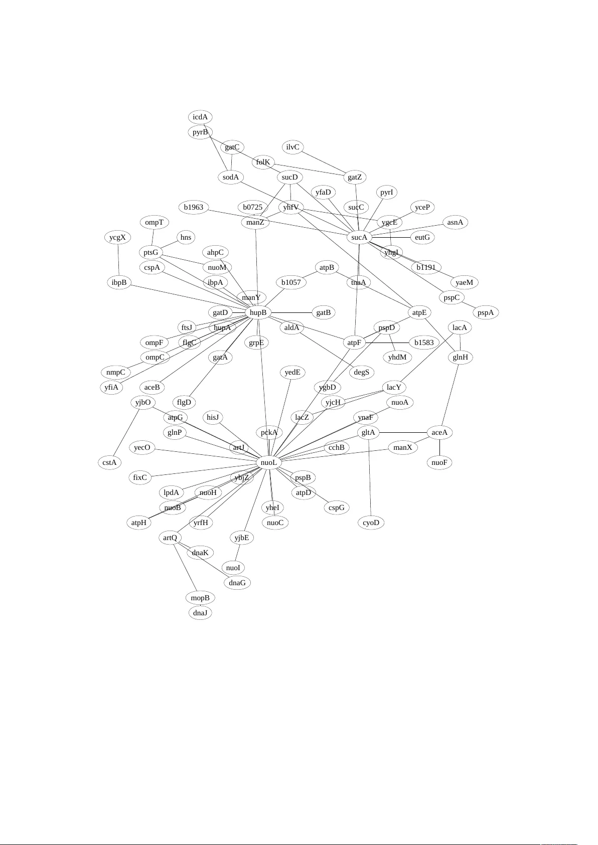
Entr opy infer ence and the James-Stein estimator , with application to nonlinear gene association networks Jean Hausser ∗ and Korbinian Strimmer † 5 October 2008; last revised 19 June 2009 Abstract W e present a pr ocedure for ef fective estimation of entropy and mutual infor - mation from small-sample data, and apply it to the problem of inferring high- dimensional gene association networks. Specifically , we develop a James-Stein-type shrinkage estimator , resulting in a pr ocedure that is highly efficient statistically as well as computationally . Despite its simplicity , we show that it outperforms eight other entropy estimation procedur es across a diverse range of sampling scenarios and data-generating models, even in cases of severe undersampling. W e illustrate the approach by analyzing E. coli gene expression data and computing an entr opy- based gene-association network from gene expression data. A computer program is available that implements the proposed shrinkage estimator . Keywords: Entropy , shrinkage estimation, James-Stein estimator , “small n , large p ” setting, mutual information, gene association network. Acknowledgments This work was partially supported by an Emmy Noether grant of the Deutsche Forschungsgemeinschaft (to K.S.). W e thank the anonymous referees and the editor for very helpful comments. ∗ Email: jean.hausser@unibas.ch; Addr ess: Bioinformatics, Biozentr um, University of Basel, Klingel- bergstr . 50/70, CH-4056 Basel, Switzerland † Email: strimmer@uni-leipzig.de; Address: Institute for Medical Informatics, Statistics and Epidemiol- ogy , University of Leipzig, Härtelstr . 16–18, D-04107 Leipzig, Germany 1 1 Introduction Entropy is a fundamental quantity in statistics and machine learning. It has a large number of applications, for example in astr onomy , cryptography , signal processing, statistics, physics, image analysis neuroscience, network theory , and bioinformatics— see, for example, Stinson (2006), Y eo and Bur ge (2004), MacKay (2003) and Strong et al. (1998). Here we focus on estimating entr opy from small-sample data, with applications in genomics and gene network inference in mind (Margolin et al., 2006; Meyer et al., 2007). T o define the Shannon entropy , consider a categorical random variable with alphabet size p and associated cell probabilities θ 1 , . . . , θ p with θ k > 0 and ∑ k θ k = 1. Throughout the article, we assume that p is fixed and known. In this setting, the Shannon entropy in natural units is given by 1 H = − p ∑ k = 1 θ k log ( θ k ) . (1) In practice, the underlying probability mass function are unknown, hence H and θ k need to be estimated from observed cell counts y k ≥ 0. A particularly simple and widely used estimator of entropy is the maximum likeli- hood (ML) estimator ˆ H ML = − p ∑ k = 1 ˆ θ ML k log ( ˆ θ ML k ) constructed by plugging the ML fr equency estimates ˆ θ ML k = y k n (2) into Eq. 1 , with n = ∑ p k = 1 y k being the total number of counts. In situations with n  p , that is, when the dimension is low and when there are many observation, it is easy to infer entropy reliably , and it is well-known that in this case the ML estimator is optimal. However , in high-dimensional pr oblems with n  p it becomes extremely challenging to estimate the entr opy . Specifically , in the “small n , large p ” regime the ML estimator performs very poorly and sever ely under estimates the true entr opy . While entropy estimation has a long history tracing back to more than 50 years ago, it is only recently that the specific issues arising in high-dimensional, undersampled data sets have attracted attention. This has lead to two recent innovations, namely the NSB algorithm (Nemenman et al., 2002) and the Chao-Shen estimator (Chao and Shen, 2003), both of which are now widely considered as benchmarks for the small-sample entropy estimation pr oblem (V u et al., 2007). Here, we introduce a novel and highly efficient small-sample entr opy estimator based on James-Stein shrinkage (Gruber, 1998). Our method is fully analytic and hence 1 In this paper we use the following conventions: log denotes the natural logarithm ( not base 2 or base 10), and we define 0 log 0 = 0. 2 computationally inexpensive. Moreover , our procedur e simultaneously provides esti- mates of the entr opy and of the cell frequencies suitable for plugging into the Shannon entropy formula (Eq. 1 ). Thus, in comparison the estimator we pr opose is simpler , very efficient, and at the same time more versatile than currently available entropy estimators. 2 Conventional Methods for Estimating Entropy Entropy estimators can be divided into two groups: i) methods, that rely on estimates of cell frequencies, and ii) estimators, that directly infer entr opy without estimating a compatible set of θ k . Most methods discussed below fall into the first group, except for the Miller-Madow and NSB appr oaches. 2.1 Maximum Likelihood Estimate The connection between observed counts y k and frequencies θ k is given by the multino- mial distribution Prob ( y 1 , . . . , y p ; θ 1 , . . . , θ p ) = n ! ∏ p k = 1 y k ! p ∏ k = 1 θ y k k . (3) Note that θ k > 0 because otherwise the distribution is singular . In contrast, there may be (and often are) zero counts y k . The ML estimator of θ k maximizes the right hand side of Eq. 3 for fixed y k , leading to the observed frequencies ˆ θ ML k = y k n with variances V ar ( ˆ θ ML k ) = 1 n θ k ( 1 − θ k ) and Bias ( ˆ θ ML k ) = 0 as E ( ˆ θ ML k ) = θ k . 2.2 Miller-Madow Estimator While ˆ θ ML k is unbiased, the corresponding plugin entropy estimator ˆ H ML is not. First order bias corr ection leads to ˆ H MM = ˆ H ML + m > 0 − 1 2 n , where m > 0 is the number of cells with y k > 0. This is known as the Miller-Madow estimator (Miller, 1955). 2.3 Bayesian Estimators Bayesian regularization of cell counts may lead to vast improvements over the ML estimator (Agresti and Hitchcock, 2005). Using the Dirichlet distribution with parameters a 1 , a 2 , . . . , a p as prior , the resulting posterior distribution is also Dirichlet with mean ˆ θ Bayes k = y k + a k n + A , 3 where A = ∑ p k = 1 a k . The flattening constants a k play the role of pseudo-counts (compar e with Eq. 2 ), so that A may be interpreted as the a priori sample size. Some common choices for a k are listed in T ab. 1 , along with r eferences to the corre- sponding plugin entropy estimators, ˆ H Bayes = − p ∑ k = 1 ˆ θ Bayes k log ( ˆ θ Bayes k ) . While the multinomial model with Dirichlet prior is standar d Bayesian folklor e (Gelman et al., 2004), there is no general agr eement r egarding which assignment of a k is best as noninformative prior —see for instance the discussion in T uyl et al. (2008) and Geisser (1984). But, as shown later in this article, choosing inappropriate a k can easily cause the resulting estimator to perform worse than the ML estimator , ther eby defeating the originally intended purpose. 2.4 NSB Estimator The NSB appr oach (Nemenman et al., 2002) avoids overr elying on a particular choice of a k in the Bayes estimator by using a more refined prior . Specifically , a Dirichlet mixture prior with infinite number of components is employed, constructed such that the r esulting prior over the entr opy is uniform. While the NSB estimator is one of the best entropy est imators available at present in terms of statistical pr operties, using the Dirichlet mixture prior is computationally expensive and somewhat slow for practical applications. 2.5 Chao-Shen Estimator Another recently proposed estimator is due to Chao and Shen (2003). This approach applies the Horvitz-Thompson estimator (Horvitz and Thompson, 1952) in combination with the Good-T uring correction (Good, 1953; Orlitsky et al., 2003) of the empirical cell probabilities to the problem of entr opy estimation. The Good-T uring-corrected frequency estimates are ˆ θ GT k = ( 1 − m 1 n ) ˆ θ ML k , a k Cell frequency prior Entropy estimator 0 no prior maximum likelihood 1/ 2 Jeffr eys prior (Jef freys, 1946) Krichevsky and T r ofimov (1981) 1 Bayes-Laplace uniform prior Holste et al. (1998) 1/ p Perks prior (Perks, 1947) Schürmann and Grassberger (1996) √ n / p minimax prior (T rybula, 1958) T able 1: Common choices for the parameters of the Dirichlet prior in the Bayesian estimators of cell frequencies, and corr esponding entr opy estimators. 4 where m 1 is the number of singletons, that is, cells with y k = 1. Used jointly with the Horvitz-Thompson estimator this results in ˆ H C S = − p ∑ k = 1 ˆ θ GT k log ˆ θ GT k ( 1 − ( 1 − ˆ θ GT k ) n ) , an estimator with remarkably good statistical pr operties (V u et al., 2007). 3 A James-Stein Shrinkage Estimator The contribution of this paper is to introduce an entropy estimator that employs James- Stein-type shrinkage at the level of cell frequencies. As we will show below , this leads to an entropy estimator that is highly effective, both in terms of statistical accuracy and computational complexity . James-Stein-type shrinkage is a simple analytic device to perform regularized high- dimensional inference. It is ideally suited for small-sample settings - the original es- timator (James and Stein, 1961) consider ed sample size n = 1. A general recipe for constructing shrinkage estimators is given in Appendix A . In this section, we describe how this approach can be applied to the specific problem of estimating cell frequencies. James-Stein shrinkage is based on averaging two very differ ent models: a high- dimensional model with low bias and high variance, and a lower dimensional model with larger bias but smaller variance. The intensity of the regularization is determined by the r elative weighting of the two models. Here we consider the convex combination ˆ θ Shrink k = λ t k + ( 1 − λ ) ˆ θ ML k , (4) where λ ∈ [ 0, 1 ] is the shrinkage intensity that takes on a value between 0 (no shrinkage) and 1 (full shrinkage), and t k is the shrinkage target. A convenient choice of t k is the uniform distribution t k = 1 p . This is also the maximum entropy tar get. Considering that Bias ( ˆ θ ML k ) = 0 and using the unbiased estimator d V ar ( ˆ θ ML k ) = ˆ θ ML k ( 1 − ˆ θ ML k ) n − 1 we obtain (cf. Appendix A ) for the shrinkage intensity ˆ λ ? = ∑ p k = 1 d V ar ( ˆ θ ML k ) ∑ p k = 1 ( t k − ˆ θ ML k ) 2 = 1 − ∑ p k = 1 ( ˆ θ ML k ) 2 ( n − 1 ) ∑ p k = 1 ( t k − ˆ θ ML k ) 2 . (5) Note that this also assumes a non-stochastic target t k . The resulting plugin shrinkage entropy estimate is ˆ H Shrink = − p ∑ k = 1 ˆ θ Shrink k log ( ˆ θ Shrink k ) . (6) Remark 1: There is a one to one correspondence between the shrinkage and the Bayes estimator . If we write t k = a k A and λ = A n + A , then ˆ θ Shrink k = ˆ θ Bayes k . This implies that the shrinkage 5 estimator is an empirical Bayes estimator with a data-driven choice of the flattening constants—see also Efron and Morris (1973). For every choice of A there exists an equivalent shrinkage intensity λ . Conversely , for every λ there exist an equivalent A = n λ 1 − λ . Remark 2: Developing A = n λ 1 − λ = n ( λ + λ 2 + . . . ) we obtain the appr oximate estimate ˆ A = n ˆ λ , which in turn r ecovers the “pseudo-Bayes” estimator described in Fienberg and Holland (1973). Remark 3: The shrinkage estimator assumes a fixed and known p . In many practical applications this will indeed be the case, for example, if the observed counts are due to discretization (see also the data example). In addition, the shrinkage estimator appears to be r obust against assuming a larger p than necessary (see scenario 3 in the simulations). Remark 4: The shrinkage approach can easily be modified to allow multiple tar gets with dif ferent shrinkage intensities. For instance, using the Good-T uring estimator (Good, 1953; Orlit- sky et al., 2003), one could setup a differ ent uniform target for the non-zero and the zero counts, respectively . 4 Comparative Evaluation of Statistical Properties In order to elucidate the relative strengths and weaknesses of the entropy estimators reviewed in the previous section, we set to benchmark them in a simulation study covering differ ent data generation pr ocesses and sampling regimes. 4.1 Simulation Setup W e compared the statistical performance of all nine described estimators (maximum likelihood, Miller -Madow , four Bayesian estimators, the proposed shrinkage estimator (Eqs. 4 – 6 ), NSB und Chao-Shen) under various sampling and data generating scenarios: • The dimension was fixed at p = 1000. • Samples size n varied from 10, 30, 100, 300, 1000, 3000, to 10000. That is, we inves- tigate cases of dramatic undersampling (“small n , lar ge p ”) as well as situations with a larger number of observed counts. The true cell probabilities θ 1 , . . . , θ 1000 were assigned in four different fashions, corre- sponding to rows 1-4 in Fig. 1 : 6 1. Sparse and heter ogeneous, following a Dirichlet distribution with parameter a = 0.0007, 2. Random and homogeneous, following a Dirichlet distribution with parameter a = 1, 3. As in scenario 2, but with half of the cells containing structural zer os, and 4. Following a Zipf-type power law . For each sampling scenario and sample size, we conducted 1000 simulation runs. In each run, we generated a new set of true cell frequencies and subsequently sampled observed counts y k from the corresponding multinomial distribution. The resulting counts y k were then supplied to the various entropy and cell frequencies estimators and the squar ed error ∑ 1000 i = k ( θ k − ˆ θ k ) 2 was computed. From the 1000 r epetitions we estimated the mean squar ed error (MSE) of the cell frequencies by averaging over the individual squared errors (except for the NSB, Miller -Madow , and Chao-Shen estimators). Similarly , we computed estimates of MSE and bias of the inferred entr opies. 4.2 Summary of Results from Simulations Fig. 1 displays the results of the simulation study , which can be summarized as follows: • Unsurprisingly , all estimators perform well when the sample size is large. • The maximum likelihood and Miller-Madow estimators perform worst, except for scenario 1. Note that these estimators are inappropriate even for moderately lar ge sample sizes. Furthermore, the bias corr ection of the Miller -Madow estimator is not particularly effective. • The minimax and 1 / p Bayesian estimators tend to perform slightly better than maximum likelihood, but not by much. • The Bayesian estimators with pseudocounts 1 / 2 and 1 perform very well even for small sample sizes in the scenarios 2 and 3. However , they are less ef ficient in scenario 4, and completely fail in scenario 1. • Hence, the Bayesian estimators can perform better or worse than the ML estimator , depending on the choice of the prior and on the sampling scenario. • The NSB, the Chao-Shen and the shrinkage estimator all are statistically very efficient with small MSEs in all four scenarios, r egar dless of sample size. • The NSB and Chao-Shen estimators ar e nearly unbiased in scenario 3. The three top-performing estimators ar e the NSB, the Chao-Shen and the prosed shrink- age estimator . When it comes to estimating the entropy , these estimators can be con- sidered identical for practical purposes. However , the shrinkage estimator is the only 7 0 200 400 600 800 0.0 0.2 0.4 0.6 Probability density bin number probability Dirichlet a=0.0007, p=1000 H = 1.11 10 50 500 5000 0.0 0.2 0.4 MSE cell frequencies sample size n estimated MSE ML 1/2 1 1/p minimax Shrink 10 50 500 5000 0 20 40 60 80 MSE entropy sample size n estimated MSE Miller−Madow Chao−Shen NSB 10 50 500 5000 0 2 4 6 8 Bias entropy sample size n estimated Bias 0 200 400 600 800 0.000 0.004 0.008 bin number probability Dirichlet a=1, p=1000 H = 6.47 10 50 500 5000 0.00 0.04 0.08 sample size n estimated MSE 10 50 500 5000 0 10 20 30 sample size n estimated MSE 10 50 500 5000 −6 −4 −2 0 sample size n estimated Bias 0 200 400 600 800 0.000 0.010 0.020 bin number probability Dirichlet a=1, p=500 + 500 zeros H = 5.77 10 50 500 5000 0.00 0.04 0.08 sample size n estimated MSE 10 50 500 5000 0 5 10 15 20 25 sample size n estimated MSE 10 50 500 5000 −5 −3 −1 0 1 sample size n estimated Bias 0 200 400 600 800 0.00 0.05 0.10 0.15 bin number probability Zipf p=1000 H = 5.19 10 50 500 5000 0.00 0.04 0.08 sample size n estimated MSE 10 50 500 5000 0 5 10 15 20 sample size n estimated MSE 10 50 500 5000 −4 −2 0 1 2 sample size n estimated Bias Figure 1: Comparing the performance of nine differ ent entropy estimators (maximum likelihood, Miller-Madow , four Bayesian estimators, the proposed shrinkage estimator , NSB und Chao-Shen) in four dif ferent sampling scenarios (r ows 1 to 4). The estimators are compared in terms of MSE of the underlying cell fr equencies (except for Miller- Madow , NSB, Chao-Shen) and according to MSE and Bias of the estimated entropies. The dimension is fixed at p = 1000 while the sample size n varies from 10 to 10000. 8 one that simultaneously estimates cell frequencies suitable for use with the Shannon entropy formula (Eq. 1 ), and it does so with high accuracy even for small samples. In comparison, the NSB estimator is by far the slowest method: in our simulations, the shrinkage estimator was faster by a factor of 1000. 5 Application to Statistical Learning of Nonlinear Gene Asso- ciation Networks In this section we illustrate how the shrinkage entropy estimator can be applied to the problem of inferring regulatory interactions between genes thr ough estimating the nonlinear association network. 5.1 From Linear to Nonlinear Gene Association Networks One of the aims of systems biology is to understand the interactions among genes and their products underlying the molecular mechanisms of cellular function as well as how disrupting these interactions may lead to different pathologies. T o this end, an extensive literatur e on the problem of gene regulatory network “r everse engineering” has developed in the past decade (Friedman, 2004). Starting from gene expression or proteomics data, differ ent statistical learning procedur es have been proposed to infer associations and dependencies among genes. Among many others, methods have been pr oposed to enable the infer ence of lar ge-scale corr elation networks (Butte et al., 2000) and of high-dimensional partial correlation graphs (Dobra et al., 2004; Schäfer and Strimmer, 2005a; Meinshausen and Bühlmann, 2006), for learning vector- autoregr essive (Opgen-Rhein and Strimmer, 2007a) and state space models (Rangel et al., 2004; Lähdesmäki and Shmulevich, 2008), and to reconstruct directed “causal” interaction graphs (Kalisch and Bühlmann, 2007; Opgen-Rhein and Strimmer, 2007b). The restriction to linear models in most of the literature is owed at least in part to the already substantial challenges involved in estimating linear high-dimensional dependency structur es. However , cell biology offers numerous examples of thr eshold and saturation effects, suggesting that linear models may not be sufficient to model gene regulation and gene-gene interactions. In order to relax the linearity assumption and to capture nonlinear associations among genes, entropy-based network modeling was recently pr oposed in the form of the ARACNE (Margolin et al., 2006) and MRNET (Meyer et al., 2007) algorithms. The starting point of these two methods is to compute the mutual information MI ( X , Y ) for all pairs of genes X and Y , where X and Y repr esent the expression levels of the two genes for instance. The mutual information is the Kullback-Leibler distance from the joint pr obability density to the product of the marginal pr obability densities: MI ( X , Y ) = E f ( x , y )  log f ( x , y ) f ( x ) f ( y )  . (7) 9 The mutual information (MI) is always non-negative, symmetric, and equals zero only if X and Y are independent. For normally distributed variables the mutual information is closely related to the usual Pearson corr elation, MI ( X , Y ) = − 1 2 log ( 1 − ρ 2 ) . Therefor e, mutual information is a natural measure of the association between genes, regar dless whether linear or nonlinear in nature. 5.2 Estimation of Mutual Information T o construct an entropy network, we first need to estimate mutual information for all pairs of genes. The entropy r epresentation MI ( X , Y ) = H ( X ) + H ( Y ) − H ( X , Y ) , (8) shows that MI can be computed from the joint and marginal entr opies of the two genes X and Y . Note that this definition is equivalent to the one given in Eq. 7 which is based on the Kullback-Leibler divergence. From Eq. 8 it is also evident that MI ( X , Y ) is the information shared between the two variables. For gene expression data the estimation of MI and the underlying entropies is challenging due to the small sample size, which r equires the use of a regularized entropy estimator such as the shrinkage approach we pr opose here. Specifically , we proceed as follows: • As a prerequisite the data must be discrete, with each measur ement assuming one of K levels. If the data are not already discr etized, we propose employing the simple algorithm of Freedman and Diaconis (1981), considering the measur ements of all genes simultaneously . • Next, we estimate the p = K 2 cell frequencies of the K × K contingency table for each pair X and Y using the shrinkage appr oach (Eqs. 4 and 5). Note that typically the sample size n is much smaller than K 2 , thus simple approaches such as ML are not valid. • Finally , from the estimated cell frequencies we calculate H ( X ) , H ( Y ) , H ( X , Y ) and the desired MI ( X , Y ) . 5.3 Mutual Information Network for E. Coli Stress Response Data For illustration, we now analyze data fr om Schmidt-Heck et al. (2004) who conducted an experiment to observe the stress response in E. Coli during expression of a recombinant protein. This data set was also used in previous linear network analyzes, for example, in Schäfer and Strimmer (2005b). The raw data consist of 4289 protein coding genes, on which measur ements were taken at 0, 8, 15, 22, 45, 68, 90, 150, and 180 minutes. W e 10 MI shrinkage estimates mutual information Frequency 0.6 0.8 1.0 1.2 1.4 1.6 1.8 0 200 400 600 800 ARACNE−processed MIs mutual information Frequency 0.0 0.5 1.0 1.5 0 1000 2000 3000 4000 5000 Figure 2: Left: Distribution of estimated mutual information values for all 5151 gene pairs of the E. coli data set. Right: Mutual information values after applying the ARACNE gene pair selection procedure. Note that the most MIs have been set to zero by the ARACNE algorithm. focus on a subset of G = 102 differ entially expressed genes as given in Schmidt-Heck et al. (2004). Discretization of the data according to Freedman and Diaconis (1981) yielded K = 16 distinct gene expression levels. From the G = 102 genes, we estimated MIs for 5151 pairs of genes. For each pair , the mutual information was based on an estimated 16 × 16 contingency table, hence p = 256. As the number of time points is n = 9, this is a strongly undersampled situation which requir es the use of a regularized estimate of entropy and mutual information. The distribution of the shrinkage estimates of mutual information for all 5151 gene pairs is shown in the left side of Fig. 2 . The right hand side depicts the distribution of mutual information values after applying the ARACNE procedure, which yields 112 gene pairs with nonzero MIs. The model selection provided by ARACNE is based on applying the information processing inequality to all gene triplets. For each triplet, the gene pair corresponding to the smallest MI is discarded, which has the effect to remove gene-gene links that correspond to indirect rather than direct interactions. This is similar to a procedur e used in graphical Gaussian models where correlations are transformed into partial correlations. Thus, both the ARACNE and the MRNET algorithms can be consider ed as devices to approximate the conditional mutual information (Meyer et al., 2007). As a result, the 112 nonzero MIs recovered by the ARACNE algorithm correspond to 11 a r t Q nuo L m o pB dna K dna G y j bE pc k A y j bO y j c H ps pB y bj Z y e c O y e dE y na F y r f H y he I a t pF hupB s uc A ps pD b1583 i bpA i bpB m a nZ o m pC pt s G o m pF m a nY y f i A s uc C s uc D y c e P y hg I y a e M y f a D t na A a r t J y g bD y hdM a t pH nuo H hupA y c g X nuo I a l dA de g S a t pE g l nH y hf V b1963 f i xC g a t D g a t Z i l v C g l t A l a c Z a c e A m a nX nuo F l a c A i c dA s o dA l a c Y a hpC a t pB b1057 b0725 c s t A c y o D dna J f l g D g a t A g a t B hi s J hns nm pC nuo M py r B c s pA ps pC a c e B a s nA a t pD a t pG b1 191 c c hB c s pG e ut G f t s J g l nP nuo A py r I f o l K y g c E nuo B nuo C f l g C g a t C g r pE l pdA o m pT ps pA Figure 3: Mutual information network for the E. coli data inferred by the ARACNE algorithm based on shrinkage estimates of entropy and mutual information. 12 statistically detectable direct associations. The corresponding gene association network is depicted in Fig. 3 . The most striking feature of the graph are the “hubs” belonging to genes hupB, sucA and nuoL. hupB is a well known DNA-binding transcriptional regulator , wher eas both nuoL and sucA are key components of the E. coli metabolism. Note that a Lasso-type procedur e (that implicitly limits the number of edges that can connect to each node) such as that of Meinshausen and Bühlmann (2006) cannot recover these hubs. 6 Discussion W e pr oposed a James-Stein-type shrinkage estimator for inferring entropy and mutual information from small samples. While this is a challenging problem, we showed that our appr oach is highly ef ficient both statistically and computationall y despite its simplicity . In terms of versatility , our estimator has two distinct advantages over the NSB and Chao-Shen estimators. First, in addition to estimating the entr opy , it also provides the underlying multinomial frequencies for use with the Shannon formula (Eq. 1 ). This is useful in the context of using mutual information to quantify non-linear pairwise dependencies for instance. Second, unlike NSB, it is a fully analytic estimator . Hence, our estimator suggests itself for applications in large scale estimation pr ob- lems. T o demonstrate its application in the context of genomics and systems biology , we have estimated an entropy-based gene dependency network from expression data in E. coli . This type of approach may prove helpful to overcome the limitations of linear models currently used in network analysis. In short, we believe the proposed small-sample entropy estimator will be a valuable contribution to the growing toolbox of machine learning and statistics pr ocedures for high-dimensional data analysis. Appendix A: Recipe For Constructing James-Stein-type Shrink- age Estimators The original James-Stein estimator (James and Stein, 1961) was proposed to estimate the mean of a multivariate normal distribution from a single ( n = 1!) vector observation. Specifically , if x is a sample from N p ( µ , I ) then James-Stein estimator is given by ˆ µ JS k = ( 1 − p − 2 ∑ p k = 1 x 2 k ) x k . Intriguingly , this estimator outperforms the maximum likelihood estimator ˆ µ ML k = x k in terms of mean squared err or if the dimension is p ≥ 3. Hence, the James-Stein estimator dominates the maximum likelihood estimator . 13 The above estimator can be slightly generalized by shrinking towar ds the component average ¯ x = ∑ p k = 1 x k rather than to zero, r esulting in ˆ µ Shrink k = ˆ λ ? ¯ x + ( 1 − ˆ λ ? ) x k with estimated shrinkage intensity ˆ λ ? = p − 3 ∑ p k = 1 ( x k − ¯ x ) 2 . The James-Stein shrinkage principle is very general and can be put to to use in many other high-dimensional settings. In the following we summarize a simple r ecipe for constructing James-Stein-type shrinkage estimators along the lines of Schäfer and Strimmer (2005b) and Opgen-Rhein and Strimmer (2007a). In short, there ar e two key ideas at work in James-Stein shrinkage: i) regularization of a high-dimensional estimator ˆ θ by linear combination with a lower-dimensional tar get estimate ˆ θ T arget , and ii) adaptive estimation of the shrinkage parameter λ from the data by quadratic risk minimization. A general form of a James-Stein-type shrinkage estimator is given by ˆ θ Shrink = λ ˆ θ T arget + ( 1 − λ ) ˆ θ . (9) Note that ˆ θ and ˆ θ T arget are two very different estimators (for the same underlying model!). ˆ θ as a high-dimensional estimate with many independent components has low bias but for small samples a potentially large variance. In contrast, the tar get estimate ˆ θ T arget is low-dimensional and therefor e is generally less variable than ˆ θ but at the same time is also more biased. The James-Stein estimate is a weighted average of these two estimators, where the weight is chosen in a data-driven fashion such that ˆ θ Shrink is improved in terms of mean squared err or relative to both ˆ θ and ˆ θ T arget . A key advantage of James-Stein-type shrinkage is that the optimal shrinkage intensity λ ? can be calculated analytically and without knowing the true value θ , via λ ? = ∑ p k = 1 V ar ( ˆ θ k ) − Cov ( ˆ θ k , ˆ θ T arget k ) + Bias ( ˆ θ k ) E ( ˆ θ k − ˆ θ T arget k ) ∑ p k = 1 E [( ˆ θ k − ˆ θ T arget k ) 2 ] . (10) A simple estimate of λ ? is obtained by r eplacing all variances and covariances in Eq. 10 with their empirical counterparts, followed by truncation of ˆ λ ? at 1 (so that ˆ λ ? ≤ 1 always holds). Eq. 10 is discussed in detail in Schäfer and Strimmer (2005b) and Opgen-Rhein and Strimmer (2007a). More specialized versions of it are treated, for example, in Ledoit and W olf (2003) for unbiased ˆ θ and in Thompson (1968) (unbiased, univariate case with 14 deterministic tar get). A very early version (univariate with zero target) even predates the estimator of James and Stein, see Goodman (1953). For the multinormal setting of James and Stein (1961), Eq. 9 and Eq. 10 reduce to the shrinkage estimator described in Stigler (1990). James-Stein shrinkage has an empirical Bayes interpr etation (Efron and Morris, 1973). Note, however , that only the first two moments of the distributions of ˆ θ T arget and ˆ θ need to be specified in Eq. 10 . Hence, James-Stein estimation may be viewed as a quasi- empirical Bayes appr oach (in the same sense as in quasi-likelihood, which also r equires only the first two moments). Appendix B: Computer Implementation The proposed shrinkage estimators of entropy and mutual information, as well as all other investigated entropy estimators, have been implemented in R (R Develop- ment Core T eam, 2008). A corresponding R package “entropy” was deposited in the R archive CRAN and is accessible at the URL http://cran.r- project.org/web/ packages/entropy / under the GNU General Public License. References Agresti, A. and Hitchcock, D. B. (2005). Bayesian inference for categorical data analysis. Statist. Meth. Appl. , 14:297–330. Butte, A. J., T amayo, P ., Slonim, D., Golub, T . R., and Kohane, I. S. (2000). Discovering functional relationships between RNA expr ession and chemotherapeutic susceptibility using relevance networks. Proc. Natl. Acad. Sci. USA , 97:12182–12186. Chao, A. and Shen, T .-J. (2003). Nonparametric estimation of Shannon’s index of diversity when there ar e unseen species. Environ. Ecol. Stat. , 10:429–443. Dobra, A., Hans, C., Jones, B., Nevins, J. R., Y ao, G., and W est, M. (2004). Sparse graphical models for exploring gene expression data. J. Multiv . Anal. , 90:196–212. Efron, B. and Morris, C. N. (1973). Stein’s estimation rule and its competitors–an empirical Bayes approach. J. Amer . Statist. Assoc. , 68:117–130. Fienberg, S. E. and Holland, P . W . (1973). Simultaneous estimation of multinomial cell probabilities. J. Amer . Statist. Assoc. , 68:683–691. Freedman, D. and Diaconis, P . (1981). On the histogram as a density estimator: L2 theory . Z. Wahrscheinlichkeitstheorie verw . Gebiete , 57:453–476. Friedman, N. (2004). Inferring cellular networks using probabilistic graphical models. Science , 303:799–805. 15 Geisser , S. (1984). On prior distributions for binary trials. The American Statistician , 38:244–251. Gelman, A., Carlin, J. B., Stern, H. S., and Rubin, D. B. (2004). Bayesian Data Analysis . Chapman & Hall/CRC, Boca Raton, 2nd edition. Good, I. J. (1953). The population frequencies of species and the estimation of population parameters. Biometrika , 40:237–264. Goodman, L. A. (1953). A simple method for improving some estimators. Ann. Math. Statist. , 24:114–117. Gruber , M. H. J. (1998). Improving Efficiency By Shrinkage . Marcel Dekker , Inc., New Y ork. Holste, D., Große, I., and Herzel, H. (1998). Bayes’ estimators of generalized entropies. J. Phys. A: Math. Gen. , 31:2551–2566. Horvitz, D. G. and Thompson, D. J. (1952). A generalization of sampling without replacement fr om a finite universe. J. Amer . Statist. Assoc. , 47:663–685. James, W . and Stein, C. (1961). Estimation with quadratic loss. In Proc. Fourth Berkeley Symp. Math. Statist. Probab. , volume 1, pages 361–379, Berkeley . Univ . California Press. Jeffr eys, H. (1946). An invariant form for the prior pr obability in estimation problems. Proc. Roc. Soc. (Lond.) A , 186:453–461. Kalisch, M. and Bühlmann, P . (2007). Estimating high-dimensional directed acyclic graphs with the PC-algorithm. J. Machine Learn. Res. , 8:613–636. Krichevsky , R. E. and T rofimov , V . K. (1981). The performance of universal encoding. IEEE T rans. Inf. Theory , 27:199–207. Lähdesmäki, H. and Shmulevich, I. (2008). Learning the structure of dynamic Bayesian networks from time series and steady state measur ements. Mach. Learn. , 71:185–217. Ledoit, O. and W olf, M. (2003). Improved estimation of the covariance matrix of stock returns with an application to portfolio selection. J. Empir . Finance , 10:603–621. MacKay , D. J. C. (2003). Information Theory , Inference, and Learning Algorithms . Cambridge University Press, Cambridge. Margolin, A., Nemenman, I., Basso, K., W iggins, C., Stolovitzky , G., Dalla Favera, R., and Califano, A. (2006). ARACNE: an algorithm for the reconstr uction of gene regulatory networks in a mammalian cellular context. BMC Bioinformatics , 7 (Suppl. 1):S7. Meinshausen, N. and Bühlmann, P . (2006). High-dimensional graphs and variable selection with the Lasso. Ann. Statist. , 34:1436–1462. 16 Meyer , P . E., Kontos, K., Lafitte, F ., and Bontempi, G. (2007). Information-theoretic inference of lar ge transcriptional regulatory networks. EURASIP J. Bioinf. Sys. Biol. , page doi:10.1155/2007/79879. Miller , G. A. (1955). Note on the bias of information estimates. In Quastler , H., editor , Information Theory in Psychology II-B , pages 95–100. Free Pr ess, Glencoe, IL. Nemenman, I., Shafee, F ., and Bialek, W . (2002). Entropy and inference, revisited. In Dietterich, T . G., Becker , S., and Ghahramani, Z., editors, Advances in Neural Information Processing Systems 14 , pages 471–478, Cambridge, MA. MIT Pr ess. Opgen-Rhein, R. and Strimmer , K. (2007a). Accurate ranking of differ entially expressed genes by a distribution-free shrinkage appr oach. Statist. Appl. Genet. Mol. Biol. , 6:9. Opgen-Rhein, R. and Strimmer , K. (2007b). From corr elation to causation networks: a simple approximate learning algorithm and its application to high-dimensional plant gene expression data. BMC Systems Biology , 1:37. Orlitsky , A., Santhanam, N. P ., and Zhang, J. (2003). Always Good T uring: asymptotically optimal probability estimation. Science , 302:427–431. Perks, W . (1947). Some observations on inverse probability including a new indiffer ence rule. J. Inst. Actuaries , 73:285–334. R Development Core T eam (2008). R: A language and environment for statistical computing . R Foundation for Statistical Computing, V ienna, Austria. ISBN 3-900051-07-0. Rangel, C., Angus, J., Ghahramani, Z., Lioumi, M., Sotheran, E., Gaiba, A., W ild, D. L., and Falciani, F . (2004). Modeling T-cell activation using gene expression profiling and state space modeling. Bioinformatics , 20:1361–1372. Schäfer , J. and Strimmer , K. (2005a). An empirical Bayes appr oach to inferring lar ge-scale gene association networks. Bioinformatics , 21:754–764. Schäfer , J. and Strimmer , K. (2005b). A shrinkage approach to large-scale covariance matrix estimation and implications for functional genomics. Statist. Appl. Genet. Mol. Biol. , 4:32. Schmidt-Heck, W ., Guthke, R., T oepfer , S., Reischer , H., Duerrschmid, K., and Bayer , K. (2004). Reverse engineering of the stress response during expression of a recombinant protein. In ?, editor , Proceedings of the EUNITE symposium, 10-12 June 2004, Aachen, Germany , volume ?, pages 407–412, ? V erlag Mainz. Schürmann, T . and Grassberger , P . (1996). Entropy estimation of symbol sequences. Chaos , 6:414–427. Stigler , S. M. (1990). A Galtonian perspective on shrinkage estimators. Statistical Science , 5:147–155. 17 Stinson, D. (2006). Cryptography: Theory and Practice . CRC Press. Strong, S. P ., Koberle, R., de Ruyter van Steveninck, R., and Bialek, W . (1998). Entropy and information in neural spike trains. Phys. Rev . Letters , 80:197–200. Thompson, J. R. (1968). Some shrinkage techniques for estimating the mean. J. Amer . Statist. Assoc. , 63:113–122. T rybula, S. (1958). Some problems of simultaneous minimax estimation. Ann. Math. Statist. , 29:245–253. T uyl, F ., Gerlach, R., and Mengersen, K. (2008). A comparison of Bayes-Laplace, Jeffreys, and other priors: the case of zero events. The American Statistician , 62:40–44. V u, V . Q., Y u, B., and Kass, R. E. (2007). Coverage-adjusted entropy estimation. Stat. Med. , 26:4039–4060. Y eo, G. and Burge, C. B. (2004). Maximum entr opy modeling of short sequence motifs with applications to RNA splicing signals. J. Comp. Biol. , 11:377–394. 18