Zero-state Markov switching count-data models: an empirical assessment

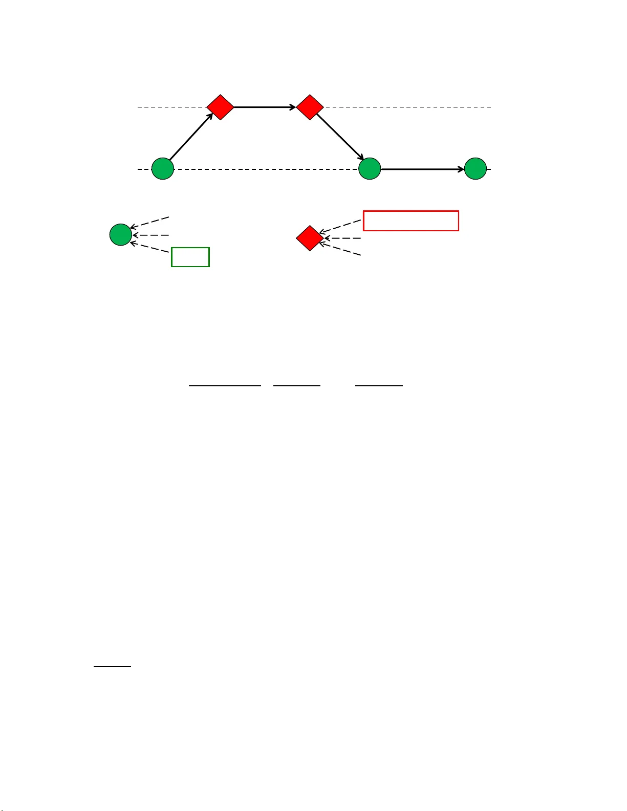
Zero-st ate Mark o v sw i tc hing count-data mo de ls: an empirical ass essmen t Natal iya V. Malyshkin a ∗ and F red L. Manner ing Scho ol of Civil Engine ering, 550 Stadium Mal l Drive, Pur due University, West L afayette, IN 47907, Unite d States Abstract In this study , a t w o-state Marko v switc hing count -d ata mo del is prop osed as an al ter- nativ e to ze ro-inflated mo dels to accoun t for the prep onderance of zeros so metimes observ ed in transp ortation count data, su c h as th e num b er of acciden ts o ccurr ing on a r oadw a y segmen t o ver some p erio d of time. F or this acciden t-frequency case, zero- inflated mo dels assume the existence of tw o states: one of th e states is a zero-acciden t coun t state, in whic h acciden t pr obabilities a re so lo w that they cann ot b e stat isti- cally distinguished f rom ze ro, and t he other stat e is a normal coun t state, in w hic h coun ts can b e non-negativ e in tegers that are generated by some counting pro cess, for example, a Poisson or negativ e b inomial. In con trast to zero-inflated m o dels, Mark o v switc hing mo dels allo w s p ecific r oadw a y segmen ts to sw itc h b et w een the t wo states ov er time. An imp ortan t adv antag e of this Marko v switc hing ap p roac h is that it allo ws f or the dir ect statistical esti mation of th e sp ecific roadw a y -segment state (i.e., zero or count state) whereas traditional zero-inflated mo dels d o not. T o demonstrate t he app licabilit y of this ap p roac h, a t wo-st ate Mark o v switc h ing neg a- tiv e b inomial mo del (estimated with Ba yesia n inference) and standard zero-inflated negativ e binomial mo d els are estimated using five-y ear accident frequ en cies on Ind i- ana interstate high w ay segmen ts. It is sho wn that t he Mark o v sw itc hing mo d el is a viable alternativ e and r esults in a sup erior statistical fit relativ e to th e zero-inflated mo dels. Key wor ds: Acciden t frequen cy count data models; zero-inflated mo dels; negativ e binomial; Mark o v switc h in g; Ba y esian; MCMC ∗ Corresp ond ing a uthor. Email addr esses: nmal yshk@purd ue.edu (Nataliy a V. Ma lysh kina), flm@ecn. purdue.ed u (F red L. Mannerin g). Preprint su bmitted to Acciden t Analysis and Prev en tion 31 Octob er 2018 1 In tr o duction The prep onderance of zeros observ ed in many coun t-data a pplications has lead researc hers to conside r the p ossibilit y that t w o states exis t ; one state that is a “zero” state (where all counts are zero) and the other that is a norma l count state that includes zeros and positive in tegers. This t wo-state assumption has led to the dev elopmen t of zero- inflated P oisson mo dels and zero-inflated neg- ativ e binomial mo dels to accoun t for p ossible ov erdisp ersion in the normal- coun t state. These zero-inflated mo dels hav e b een applied to a n umber of fields of study . F or example, Lam b ert (1992) used a zero-inflated Pois son mo del to study man ufacturing defects. Lam b ert argued that unobserv ed c hanges in the pro cess caused man ufacturing defects t o mo v e ra ndo mly b et w een a state that w as n ear p erfect (the zero state where defects were extremely rare) and an im- p erfect s tate whe r e defects w ere p ossible but not inevitable (t he normal coun t state). Lam b erts empirical assessmen t demonstrated that the zero-inflated mo deling approac h fit the data m uc h b etter than the standard P oisson. In other w ork, v an den Bro ek (1995) pro vided an application of the zero-inflated P oisson to the frequency of urinary tract infections in men diagnosed with the h uman immunodeficiency virus (HIV). In this case, it w as p o stulated that a zero-infection state existed fo r a p ortion o f the patien t p opulation a nd t ha t this state generated a larg e num b er of zeros in the frequency data, whic h w as supp orted by the statistical findings. Also, Bohning et al. (1999) successfully applied the zero-inflated P oisson to study the frequency of den tal deca y in P ortugal. The frequency o f v ehicle acciden ts on a section of highw a y or a t an inte rsection (o ver some time p erio d) often exhibit excess zeros. Similar to the literature discusse d ab ov e, the exces s of zeros observ ed in the data could p oten tia lly b e explained b y the existence of a tw o-state pro cess for acciden t data genera- tion (Shank ar et al., 1997; Carson and Mannering, 2001; Lee and Mannering , 2002). In this case, roadw ay se g men ts can belong t o one of t w o states: a zero-acciden t state (where zero acciden ts are exp ected) and a no r mal-coun t state, in whic h acciden ts can happ en and acciden t frequencies are generated b y s o me giv en counting pro cess (P oisson or negativ e binomial). T o account for the tw o-state phenomena, zero-inflated Poisson (ZIP) and zero-inflated nega- tiv e binomial (ZINB) mo dels hav e b een used in a n um b er o f roa dw ay saf ety studies (Miaou, 1994; Shank ar et al., 1997; W ashington et al., 200 3). Thes e mo dels explicitly accoun t for an existence of the t w o states for acciden t data generation and a llo w mo deling of the probabilities of b eing in these states. An application of ZIP and ZINB mo dels w as an empirical adv ance in statisti- cal mo deling of acciden t frequencies. Ho w ever, altho ug h zero-inflated mo dels ha ve b ecome p opular in a num b er of fields, they suffer from t w o imp ort an t dra wback s. First, these mo dels do not deal directly with the states of ro a d- 2 w ay segmen ts, instead they consider probabilities of b eing in these states. As a result, zero-inflat ed mo dels do not allow a direct statistical estimation of whether individual roadw ay segmen ts are in the zero or normal coun t state. F o r example, supp ose a giv en r o adw ay segmen t has zero acciden ts observ ed o ve r a giv en time interv al. This segmen t could truly b e in the zero-a cciden t coun t state, or it ma y be in the normal-coun t state and just happened to ha v e zero acciden ts o v er the considered time interv al (Shank ar et al., 1997). Distin- guishing betw een these t w o p ossibilities is not straightforw ard in z ero-inflated mo dels. The second draw back of zero-inflated mo dels is that, a lthough they allo w roadwa y segmen ts to b e in differen t states during different observ ation p erio ds, zero-inflated models do not explicitly conside r switc hing b y the road- w ay segmen ts b et w een the states ov er time. This switc hing is impo rtan t f rom the theoretical point of vie w b ecause it is unreas o nable to exp ect an y r o adw ay segmen t t o be in the zero-acciden t all the time and to hav e the long-term mean a cciden t frequency equal t o zero (Lord et a l., 2005). In this study , w e prop ose t w o-state Marko v switc hing coun t-data mo dels that consider the ze ro-acciden t state a nd the normal-coun t state of roadw ay safety . Similar to zero-inflated mo dels, Mark ov switc hing mo dels are in tended to ex- plain the prep onderance o f zeros observ ed in acciden t count data. How ev er, in con trast to zero-inflated mo dels, Marko v switc hing mo dels allo w a direct statistical estimation of the states roadwa y segmen ts a re in at sp ecific p oin ts in time and explicitly consider changes in these states ov er time. 2 Mo del sp ecification Tw o-state Mark ov switc hing count-data mo dels of acciden t frequencies w ere first presen ted in Malyshkina et al. (2009). F ollow ing that pap er, w e note that, although there are sev eral ma jor differences betw een Malyshk ina et al. (2009) and this study , man y ideas a nd statistical estimation metho ds dev elop ed in Malyshkina et al. (2009) apply in this study as w ell. In that pap er, t w o states w ere assumed to exist but b oth w ere true coun t states (i.e., a zero-count state did not exist). In the curren t pap er, w e tak e a differen t approach and consider the case where o ne of the states is a zero state and the other is a true coun t state and that individual roa dwa y segmen ts mo v e b etw een these t wo states ov er time. This differs f r o m Malyshkina et al. (2009) in that their mo del assumes t w o true-count states and that all roa dwa y segments are in the same state at the same time. T o sho w t his mo del, w e not e that Mark o v switc hing mo dels are parametric and can b e fully sp ecified by a lik eliho o d function f ( Y | Θ , M ), whic h is the conditional probability distribution of the v ector of all observ ations Y , given the v ector o f all parameters Θ o f mo del M . In our study , w e observ e the 3 n umber of acciden ts A t,n that o ccur on the n th roadw ay segmen t during time p erio d t . Th us Y = { A t,n } includes all acciden ts observ ed on all r oadw ay segmen ts ov er all time p erio ds. Here n = 1 , 2 , . . . , N and t = 1 , 2 , . . . , T , where N is the total n um b er of roadw ay segmen ts observ ed (it is assumed to b e constan t o v er time) and T is the total num b er of t ime perio ds. Mo del M = { M , X t,n } includes the mo del’s name M (f o r example, M = “ZIP” or “Z INB”) and the ve ctor X t,n of a ll roa dwa y segmen t c haracteristic v ariables (segmen t length, curv e c haracteristics, gra des, pa veme nt prop erties, and so on). T o define the likelihoo d function, we introduce an unobserv ed (laten t ) state v a riable s t,n , whic h determines the state of the n th roadw ay segmen t during time p erio d t . Without loss of g eneralit y , it is assumed assume tha t the state v a riable s t,n can tak e on the following tw o v alues: s t,n = 0 corresp onds to the zero- a cciden t state, and s t,n = 1 corresp onds to the normal-count state ( n = 1 , 2 , . . . , N and t = 1 , 2 , . . . , T ). It is further assumed that, for e ac h road- w ay segmen t n , the state v ariable s t,n follo ws a stationary tw o-state Mark ov c hain process in time, 1 whic h can b e sp ecified by time-indep enden t transition probabilities as P ( s t +1 ,n = 1 | s t,n = 0) = p ( n ) 0 → 1 , P ( s t +1 ,n = 0 | s t,n = 1) = p ( n ) 1 → 0 . (1) Here, for example, P ( s t +1 ,n = 1 | s t,n = 0) is the conditional probability of s t +1 ,n = 1 at time t + 1, g iv en that s t,n = 0 at time t . T ransition probabilities p ( n ) 0 → 1 and p ( n ) 1 → 0 are unknow n parameters to b e estimated f rom acciden t data ( n = 1 , 2 , . . . , N ). Th e stationary unconditional probabilities of states s t,n = 0 and s t,n = 1 are ¯ p ( n ) 0 = p ( n ) 1 → 0 / ( p ( n ) 0 → 1 + p ( n ) 1 → 0 ) and ¯ p ( n ) 1 = p ( n ) 0 → 1 / ( p ( n ) 0 → 1 + p ( n ) 1 → 0 ) resp ectiv ely . 2 If p ( n ) 0 → 1 < p ( n ) 1 → 0 , then ¯ p ( n ) 0 > ¯ p ( n ) 1 and, on a ve rage, f o r roadw ay segmen t n state s t,n = 0 o ccurs more frequen tly than state s t,n = 1. If p ( n ) 0 → 1 > p ( n ) 1 → 0 , then state s t,n = 1 o ccurs more frequen t ly for segmen t n . 3 Next, consider a tw o-state Mark ov switc hing negativ e binomial (MSNB) mo del that assumes a negative binomial (NB) data-generating pro cess in the normal- coun t state s t,n = 1. With this, the probabilit y of A t,n acciden ts o ccurring on roadw ay segmen t n during time p erio d t is 1 Mark o v prop erty means th at the probability distribution of s t +1 ,n dep end s only on the v alue s t,n at time t , but not on the previous history s t − 1 , s t − 2 , . . . . S tationarit y of { s t,n } is in the statist ical sense. 2 These can b e found from statio n arit y conditions ¯ p ( n ) 0 = [1 − p ( n ) 0 → 1 ] ¯ p ( n ) 0 + p ( n ) 1 → 0 ¯ p ( n ) 1 , ¯ p ( n ) 1 = p ( n ) 0 → 1 ¯ p ( n ) 0 + [1 − p ( n ) 1 → 0 ] ¯ p ( n ) 1 and ¯ p ( n ) 0 + ¯ p ( n ) 1 = 1. 3 Here, Eq. (1) is a significan t d eparture from Malyshkina et al. (2009) in that in- dividual roadwa y segmen ts can b e in different s tates at the same time (i.e., the state v ariable is subscrip ted by roadw ay segmen t n ). Also, in contrast to Malyshkina et al. (2009), here we d o n ot restrict state s t,n = 0 to b e more frequent th an state s t,n = 1. 4   0 s ) ( 1 0 n p o ) ( 0 1 ) ( 1 1 1 n n p p o o  ) ( 0 1 n p o ) ( 1 0 ) ( 0 0 1 n n p p o o  1 s ) , | ( ) 0 ( ) 0 ( , D ȕ n t A NB or ) | ( ) 0 ( , ȕ n t A P o r ) ( , n t A I ) , | ( ) 1 ( ) 1 ( , D ȕ n t A NB o r ) | ( ) 1 ( , ȕ n t A P o r ) ( , n t A I 1 , 2  n t s 0 , 3  n t s 1 , 1  n t s 0 , n t s 0 , 1  n t s Fig. 1. Graphical demonstration of a t w o-state Mark o v switc hing mo d el. P ( A ) t,n =      I ( A t,n ) if s t,n = 0 N B ( A t,n ) if s t,n = 1 , (2) I ( A t,n ) = { 1 if A t,n = 0 and 0 if A t,n > 0 } , (3) N B ( A t,n ) = Γ( A t,n + 1 /α ) Γ(1 /α ) A t,n ! 1 1 + αλ t,n ! 1 /α αλ t,n 1 + αλ t,n ! A t,n , (4) λ t,n = exp( β ′ X t,n ) , t = 1 , 2 , . . . , T , n = 1 , 2 , . . . , N . (5) Here, Eq. (3) is t he probability mass function that reflects the fact tha t acci- den ts neve r happ en in the zero-acciden t state s t,n = 0. 4 Eq. (4) is the standard negativ e binomial proba bilit y mass function, Γ( ) is the gamma function, and prime means transp ose (so β ′ is the tr a nsp ose of β ). P arameter v ector β and the ov er-dispersion parameter α ≥ 0 are unkno wn estimable mo del parame- ters. 5 Scalars λ t,n are the a cciden t rates in the normal- coun t state. W e set the first compo nent o f X t,n to unit y , and, therefore, the fir st comp onen t of β is the in tercept. A tw o-state Mark ov switc hing mo del of acciden t frequencies is gr aphically demonstrated in Figure 1 . In the tw o states s = 0 and s = 1 show n in the figure, the acciden t frequency data are generated b y t wo differen t pro cesse s, sho wn by the circles (for state s = 0) and the diamonds (fo r s = 1). In this study , we assume that acciden t frequency is generated according to the zero- acciden t distribution I ( A t,n ) in state s = 0, and according to the standard 4 Although Eq. (3) formally assumes s t,n = 0 to b e a ze r o-acciden t s tate, in whic h acciden ts nev er happ en, this state can b e view ed as an approximat ion for a nearly safe state, in whic h the a verage acciden t r ate is negligible ( λ t,n ≪ 1) and acciden ts are extremely rare (o v er the considered time p erio d ). 5 T o ens u re that α is non-negativ e, w e estimate its logarithm instead of it. 5 negativ e binomial distribution N B ( A t,n ) in state s = 1 (these t w o distributions are outlined b y the b o xes in Figure 1). The state v ariable s t,n follo ws a Mark ov pro cess o ve r time, with transition probabilities p ( n ) 0 → 0 , p ( n ) 0 → 1 , p ( n ) 1 → 0 and p ( n ) 1 → 1 , as sho wn in Figure 1. If acciden t ev en ts are assumed to b e indep enden t , the lik eliho o d function is f ( Y | Θ , M ) = T Y t =1 N Y n =1 P ( A ) t,n . (6) Here, b ecause the state v ariables s t,n are unobserv able, the v ector of all es- timable parameters Θ mus t include all states, in addition to all mo del param- eters ( β -s, α ) and transition probabilities. Th us, Θ = [ β ′ , α , p (1) 0 → 1 , . . . , p ( N ) 0 → 1 , p (1) 1 → 0 , . . . , p ( N ) 1 → 0 , S ′ ] ′ , where v ector S = [( s 1 , 1 , ..., s T , 1 ) , . . . , ( s 1 ,N , ..., s T ,N )] ′ has length T × N and con tains a ll state v alues. Eqs. (1)-(6) define the tw o-state Marko v switc hing negativ e binomial ( MSNB) mo del considered here. Note tha t in this mo del the estimable state v ariables s t,n explicitly sp ecify the states of a ll roadwa y segmen ts n = 1 , 2 , . . . , N during all time p erio ds t = 1 , 2 , . . . , T . In t his study , in addition to the MSNB mo del, w e also consider the standard zero-inflated negative binomial (ZINB) mo dels. In t his case, the probability of A t,n acciden ts o ccurring is (W ashington et al., 2003) P ( A ) t,n = q t,n I ( A t,n ) + (1 − q t,n ) N B ( A t,n ) , (7) q t,n = 1 1 + e − τ log λ t,n , (8) q t,n = 1 1 + e − γ ′ X t,n , (9) where w e use t w o differen t sp ecifications for the probabilit y q t,n that the n th roadw ay segmen t is in the ze ro-acciden t state during time p erio d t . The right- hand-side of Eq. (7 ) is a mixture of zero-acciden t dis tribution I ( A t,n ) giv en b y Eq. (3) and negat ive binomial distribution N B ( A t,n ) given by Eq. (4). Scalar τ and ve ctor γ are estimable mo del parameters. Acciden t rate λ t,n is given b y Eq. ( 5 ). W e call “ZINB- τ ” the mo del sp ecified b y Eqs . (7) and (8 ) . W e call “ZINB- γ ” the mo del sp ecified b y Eqs. (7) and (9) . Note that q t,n dep ends on the estimable mo del parameters and giv es the probabilit y of b eing in the zero-acciden t state s t,n = 0, but it is not an estimable pa rameter b y itself and do es not explicitly sp ecify the state v alue s t,n . 6 3 Mo del estimation metho ds Statistical estimation of Mark o v switc hing mo dels is complicated b y unobserv- abilit y of the state v ariables s t,n . 6 As a result, the traditio nal maxim um lik eli- ho o d estimation (MLE) procedure is of v ery limited use for Mark ov switc hing mo dels. Instead, a Bay esian inference approach is used. Giv en a mo del M with likelihoo d function f ( Y | Θ , M ), the Ba y es formula is f ( Θ | Y , M ) = f ( Y , Θ |M ) f ( Y |M ) = f ( Y | Θ , M ) π ( Θ |M ) R f ( Y , Θ |M ) d Θ . (10) Here f ( Θ | Y , M ) is the p osterior pro babilit y distribution of mo del parameters Θ conditional o n the observ ed data Y and mo del M . F unction f ( Y , Θ |M ) is the joint probability distribution of Y and Θ give n mo del M . F unction f ( Y |M ) is the marginal likelihoo d function – the pro babilit y distribution of data Y given mo del M . F unction π ( Θ |M ) is the prior probability distribution of parameters tha t reflects prior knowle dge ab out Θ . The intuition b ehind Eq. (10) is straightforw ard: g iv en mo del M , the p osterior distribution accoun ts for b oth the observ a tions Y a nd o ur prior kno wledge of Θ . In our study (and in most practical studies), the direct application of Eq. (10) is not feasible b ecause the parameter v ector Θ con ta ins to o many comp onen ts, making integration o v er Θ in Eq. (10 ) ex t r emely difficult. Ho w ev er, the p oste- rior distribution f ( Θ | Y , M ) in Eq. (10) is kn o wn up to its normalization con- stan t, f ( Θ | Y , M ) ∝ f ( Y | Θ , M ) π ( Θ |M ). As a result, we use Marko v Chain Mon te Carlo ( MCMC) sim ulations, whic h prov ide a con ven ien t a nd practi- cal computational metho dolog y for sampling from a probability distribution kno wn up to a constan t (the p osterior distribution in our case). Giv en a large enough p o sterior sample of parameter vec tor Θ , any p osterior expectation and v a riance can be f ound and Bay esian inference can b e readily applied. A reader in terested in details is referred to Malyshkina (2008), where w e comprehen- siv ely describe our c hoice of the prior distribution π ( Θ |M ) and the MCMC sim ulation alg orithm. 7 W e used MA TLAB language for prog ramming a nd running the MCMC sim ulations. F o r comparison of different mo dels we use a formal Bay esian approach. Let there b e t w o mo dels M 1 and M 2 with parameter v ectors Θ 1 and Θ 2 resp ec- tiv ely . Assuming t hat we ha v e equal preferences of these mo dels, their prior 6 Belo w we w ill h a ve fiv e time p erio ds ( T = 5) and 335 roadwa y segmen ts ( N = 335). In this case, there are 2 T N = 2 1675 p ossible com binations for v alue of ve ctor S = [( s 1 , 1 , ..., s T , 1 ) , . . . , ( s 1 ,N , ..., s T ,N )] ′ . 7 Our priors for α , β -s, p 0 → 1 and p 1 → 0 are fl at or nearly flat, while the prior f or the states S reflects the Mark o v pro cess prop erty , sp ecified b y Eq. (1). 7 probabilities are π ( M 1 ) = π ( M 2 ) = 1 / 2. In this case, the ratio of the mo dels’ p osterior probabilities, P ( M 1 | Y ) and P ( M 2 | Y ), is equal to the Ba y es fac- tor. The later is defined as the ratio o f the mo dels’ marginal lik eliho o ds (see Kass a nd Raft ery, 1995). Th us, w e hav e P ( M 2 | Y ) P ( M 1 | Y ) = f ( M 2 , Y ) /f ( Y ) f ( M 1 , Y ) /f ( Y ) = f ( Y |M 2 ) π ( M 2 ) f ( Y |M 1 ) π ( M 1 ) = f ( Y |M 2 ) f ( Y |M 1 ) , (11) where f ( M 1 , Y ) and f ( M 2 , Y ) ar e t he jo in t distributions of the mo dels and the data, f ( Y ) is the unconditional distribution of the data. As in Malyshkina et al. (2009), to calculate the margina l likelihoo ds f ( Y | M 1 ) and f ( Y |M 2 ), w e use the harmonic mean formula f ( Y |M ) − 1 = E [ f ( Y | Θ , M ) − 1 | Y ], where E ( . . . | Y ) means p osterior exp ectation calculated by using the p osterior dis- tribution. If the ratio in Eq. (11) is larger than one, then mo del M 2 is fa vored, if the ra t io is less than one, then mo del M 1 is f av ored. An adv a n tage of the use of Ba y es factors is that it has an inheren t p enalt y for including to o ma ny parameters in the mo del and guards ag ainst ov erfitting. T o ev aluate the perfo r ma nce of mo del {M , Θ } in fitting the observ ed data Y , w e carry o ut a χ 2 go o dness-of-fit test (Maher and Summersgill, 19 9 6; Co w an , 1998; W o o d, 2002; Press et al., 2007). W e p erform this test by Monte Carlo sim ulations to find the distribution o f the χ 2 quan tity , whic h measures the dis- crepancy b etw een the observ ations and the mo del predictions (Co wan, 1998). This distribution is then used to find the go o dness-of-fit p-v alue, whic h is the probabilit y tha t χ 2 exceeds the observ ed v alue of χ 2 under the hypothesis that the mo del is true (the observ ed v alue of χ 2 is calculated b y using the o bserv ed data Y ). F or additional details, please see Malyshkina (2008). 4 Empirical results Data are used from 5769 acciden ts that we r e observ ed on 335 in terstate hig h- w ay segmen ts in Indiana in 1 995-199 9. W e use ann ual time perio ds, t = 1 , 2 , 3 , 4 , T = 5 in t o tal. 8 Th us, for each roadw ay segmen t n = 1 , 2 , . . . , N = 335 the state s t,n can c hange ev ery y ear. F o ur t yp es of acciden t frequency mo dels are estimated: (1) First, for t he purp ose of explanatory v ariable selection, w e estimate an auxiliary standard negativ e binomial (NB) mo del, whic h is not rep orted here. W e estimate this mo del b y maxim um lik eliho o d estimation (MLE). T o obtain a standard NB mo del, w e c ho ose explanatory v ariables and 8 W e also considered quarterly time p eriod s and obtained qu alitativ ely similar re- sults (not rep orted here). 8 their dummies b y using the Ak aike Information Criterion (AIC) 9 and the 5% statistical significance lev el for the tw o-tailed t-test (for details on our v ariable selection metho ds, see Malyshkina, 20 06). In or der to mak e a comparison of explanatory v ariable effects in differen t mo dels straigh tfo rw ard, in a ll other mo dels, describ ed b elow, w e use only those explanatory v ariables that en ter the standard NB mo del. 10 (2) W e estimate the standard ZINB- τ mo del, sp ecified b y Eqs . (6)–(8). First, w e estimate this mo del by ma ximum lik eliho o d estimation (MLE) and use the 5% statistical significance lev el for ev aluation of the statistical significance of eac h β -para meter. Second, w e estimate the same Z INB- τ mo del b y the Ba yes ia n inference approach and MCMC sim ulations. As one exp ects, the Ba y esian-MCMC estimation results turned out to b e similar t o the MLE estimation results fo r the ZINB- τ mo del. (3) W e estimate the standard ZINB- γ mo del, sp ecified by Eqs. (6), (7) and ( 9). First, w e estimate this mo del b y MLE and use the 5% statistical sig- nificance level for ev aluation of the statistical significance of eac h β - parameter. Se cond, w e estimate the same ZINB- γ mo del b y the Ba yes ia n inference a pproac h and MCMC sim ulatio ns. The Bay esian-MCMC and the MLE estimation results for t he ZINB- γ mo del turned out to b e sim- ilar. (4) W e estimate the t wo-state Marko v switc hing negativ e binomial (MSNB) mo del, sp ecified by Eqs. (1)-(6), b y the Bay esian-MCMC metho ds. W e consecutiv ely construct and us e 60%, 85% and 95% Ba y esian credible in- terv a ls fo r ev aluation of the statistical significance of each β - parameter in the MSNB mo del. As a result, in the final MSNB mo del some com- p onen ts of β are restricted to zero. 11 No restriction is imp osed on t he o ve r-disp ersion para meter α , whic h turns out to b e significan t anyw a y . The mo del estimation results for acciden t frequencies are giv en in T able 1. Con tinuous mo del par a meters, β -s and α , are giv en together with their 95% confidence in terv als (if MLE) or 95% credible in terv als (if Bay esian-MCMC), refer to the sup erscript and subscript n umbers adjacen t t o parameter esti- mates in T able 1. 12 T able 2 giv es summary statistics of all ro adw ay segmen t 9 Minimization of AI C = 2 K − 2 LL , w ere K is the num b er of fr ee con tinuous mo del parameters and LL is the log-lik eliho o d, ensures an optimal choice of explanatory v ariables in a mod el and a voids o ve r fitting (Tsay, 2 002; W ashington et al., 200 3). 10 A formal Ba ye s ian approac h to mo del v ariable selection is b ased on ev aluation of mo d el’s marginal lik eliho o d and the Ba yes factor (11). Unfortun ately , b ecause MCMC sim u lations are compu tationally exp ensiv e, ev aluation of marginal like li- ho o ds for a large n u mb er of tr ial mo dels is not feasible in our study . 11 A β -parameter is restricted to zero if it is statistically insignifican t. A 1 − a credible in terv al is c hosen in suc h w ay that the p osterior probabilities of b eing b elo w and ab o ve it are both equal to a/ 2 (w e use significance leve ls a = 40% , 15% , 5%). 12 Note t h at MLE assumes asymptotic n orm alit y of th e estimates, resulting in con- fidence interv als b eing symmetric around the m eans (a 95% confidence in terv al is 9 c haracteristic v ariables X t,n (except t he interce pt). The estimation results sho w that the MSNB mo del is strongly fa vored b y the empirical data, a s compared t o the standard ZINB mo dels. Indeed, from T a- ble 1 we see that the MSNB mo del provides considerable, 335 . 6 9 and 263 . 1 2 , impro ve ments of the logarithm of the marginal lik eliho o d of the data as com- pared to the Z INB- τ and ZINB- γ mo dels. 13 Th us, from Eq. (11), w e find that, giv en the acciden t data, the p osterior probabilit y of the MSNB mo del is larg er than the probabilities of the ZINB- τ and ZINB- γ mo dels b y e 335 . 69 and e 263 . 12 resp ectiv ely . 14 Let us now consider the maxim um lik eliho o d estimation (MLE) o f the standard ZINB- τ and ZINB- γ mo dels and an imaginary MLE estimation of the MSNB mo del. Referring to T able 1, the MLE gav e maxim um log-like liho o d v alues − 2502 . 67 and − 2426 . 54 for the ZINB- τ and ZINB- γ mo dels. The maxim um log-lik eliho o d v alue observ ed during our MCMC simulations for the MSNB mo del is equal to − 2049 . 45. An imaginar y MLE, a t its con vergenc e, w ould giv e MSNB log-lik eliho o d v a lue tha t w ould b e eve n larger than this observ ed v a lue. Therefore, the MSNB mo del, if estimated by the MLE, would pro vide v ery large, at least 4 53 . 22 and 3 7 7 . 09, improv emen ts in the maxim um log- lik eliho o d v alue ov er the Z INB- τ and ZINB- γ mo dels. These impro vem ents w ould come with no increase or a decrease in the n um b er of free con t inuous mo del parameters ( β -s, α , τ , γ -s) that en ter the likelihoo d function. ± 1 . 96 standard d eviations around the mean). I n contrast, Ba y esian e stimation do es not requir e this assumption, and p osterior distributions of parameters and Bay esian credible in terv als are usu ally non-symmetric. 13 W e use the harmonic mean formula to calc ulate the v alues and the 95% confi dence in terv als of th e log-marginal-lik eliho o ds giv en in T able 1 . The confidence int er v als are calculated by b o otstrap simulatio ns. F or details, see Malyshkina et al. (2009) or Malyshkina (2008). 14 There are other frequen tly used mo del comparison criteria, for examp le, the de- viance information criterion, DIC = 2 E [ D ( Θ ) | Y ] − D ( E [ Θ | Y ]), w here deviance D ( Θ ) ≡ − 2 ln[ f ( Y | Θ , M )] (Rob ert , 200 1). Mo dels with smaller DIC are fa v ored to mo dels with large r DIC. W e find DIC v alues 5037 . 3 , 4891 . 4 , 4261 . 5 f or the Z I NB- τ , ZINB- γ and MSNB mod els resp ectiv ely . This means that th e MS NB mo del is fa- v ored o ve r the standard ZINB mo dels. How ev er, DIC is theoreticall y based on the assumption of asymptotic multiv ariate normalit y of the p osterior distribution, in whic h case DIC reduces to AIC (Spiegelhalter et al., 2002). As a r esu lt, we pr efer to rely on a mathematically r igorous and formal Ba ye s factor app roac h to mo del selection, as giv en by Eq. (1 1 ). 10 T able 1 Estimation results for mod els of acci d en t frequency (the sup ers cript a nd subscript n umb ers to the righ t of individu al parameter estimates are 95% co nfidence/credible inte rv als – see text for further explanation) V ariabl e ZINB- τ a ZINB- γ b MSNB c b y MLE b y MCMC by ML E b y MCMC b y MCMC β - and α -parameters in Eq. (5) In tercept (constan t term) − 15 . 0 − 12 . 5 − 17 . 5 − 15 . 2 − 13 . 0 − 17 . 4 − 11 . 6 − 8 . 32 − 14 . 8 − 11 . 6 − 8 . 29 − 14 . 6 − 17 . 3 − 13 . 0 − 21 . 3 Acciden t o ccurring on interstate s I-70 or I-164 (dummy) − . 683 − . 570 − . 797 − . 685 − . 575 − . 794 − . 715 − . 602 − . 829 − . 715 − . 593 − . 836 − . 734 − . 617 − . 850 Pa v emen t qualit y i ndex (PQI) a verage d − . 0122 − . 0189 − . 00550 − . 0122 − . 00562 − . 0188 − . 0140 − . 00627 − . 0217 − . 0143 − . 00643 − . 0221 − . 0163 − . 00850 − . 0240 Logarithm of road segmen t l ength (in m iles) . 791 . 832 . 751 . 791 . 829 . 754 . 929 . 978 . 880 . 939 . 993 . 886 . 887 . 929 . 845 Number of r amps on the viewing side p er l ane per mile . 226 . 300 . 153 . 227 . 306 . 149 . 298 . 387 . 209 . 304 . 394 . 214 . 317 . 404 . 230 Number of l anes on a roadw ay – – – – 1 . 19 2 . 04 . 386 Median config uration i s depressed (dummy) . 184 . 288 . 0795 . 183 . 282 . 0839 . 201 . 319 . 0820 . 202 . 325 . 0781 – Median barrier presence (dumm y) − 1 . 43 − 1 . 22 − 1 . 64 − 1 . 43 − 1 . 14 − 1 . 72 – – − 1 . 69 − 1 . 00 − 2 . 46 Width of the in terior shoulder i s less that 5 feet (dummy) . 323 . 443 . 202 . 323 . 434 . 211 . 435 . 572 . 297 . 437 . 569 . 307 . 374 . 505 . 243 Outside shoulder w i dth (in feet) − . 0480 − . 0196 − . 0764 − . 0478 − . 0207 − . 0749 − . 0532 − . 0176 − . 0887 − . 0532 − . 020 − . 0867 − . 0537 − . 0214 − . 0862 Outside barrier is absen t (dummy) – – − . 245 − . 117 − . 373 − . 245 − . 101 − . 389 − . 264 − . 124 − . 403 Ave r age ann ual daily traffic (AADT ) − 4 . 07 − 3 . 17 − 4 . 97 × 10 − 5 − 4 . 14 − 3 . 31 − 5 . 04 × 10 − 5 − 1 . 93 − 3 . 21 − 6 . 50 × 10 − 5 − 1 . 91 − 3 . 16 − 5 . 83 × 10 − 5 − 3 . 78 − 2 . 02 − 5 . 26 × 10 − 5 Logarithm of a verage ann ual dail y traffic 1 . 89 2 . 17 1 . 61 1 . 91 2 . 16 1 . 67 1 . 52 1 . 88 1 . 15 1 . 52 1 . 86 1 . 15 1 . 95 2 . 34 1 . 49 Number of br idges per mil e – – – – − . 0214 − . 00164 − . 0428 Maximum of recipro cal v alues of horizon tal curv e radii (in 1 / mile) − . 140 − . 0710 − . 209 − . 141 − . 0734 − . 208 − . 134 − . 0559 − . 213 − . 138 − . 0593 − . 217 − . 106 − . 0289 − . 183 Pe r cen tage of single unit trucks (daily a verage) 1 . 23 1 . 84 . 624 1 . 23 1 . 82 . 646 1 . 32 1 . 96 . 693 1 . 32 1 . 96 . 691 1 . 29 1 . 90 . 688 Number of changes per v ertical profile along a roadwa y segment . 0555 . 0930 . 0180 . 0562 . 0903 . 0226 – – – Ove r -disp ersion parameter α i n NB mo dels . 144 . 183 . 105 . 150 . 192 . 114 . 130 . 168 . 0925 . 142 . 185 . 105 . 114 . 147 . 0847 11 T able 1 (Con tinued) V ariabl e ZINB- τ a ZINB- γ b MSNB b y MLE by MCMC b y MLE by MC MC b y MCMC c τ - and γ -parameters in Eqs. (8) and (9) The model parameter τ in Eq. (8) − 1 . 72 − 1 . 45 − 2 . 00 − 1 . 73 − 1 . 50 − 1 . 98 – – – In tercept (constan t term) – – 23 . 1 41 . 3 4 . 99 26 . 5 47 . 0 10 . 9 – Logarithm of road segmen t l ength (in m iles) – – − 1 . 34 − . 942 − 1 . 73 − 1 . 4 − 1 . 03 − 1 . 83 – Median barrier presence (dumm y) – – 3 . 97 4 . 86 3 . 08 4 . 16 5 . 20 3 . 27 – Ave r age ann ual daily traffic (AADT ) – – 9 . 23 15 . 1 3 . 35 × 10 − 5 10 . 5 17 . 4 5 . 72 × 10 − 5 – Logarithm of a verage ann ual dail y traffic – – − 2 . 88 − . 901 − 4 . 86 − 3 . 28 − 1 . 59 − 5 . 57 – Mean acciden t r ate ( λ t,n for NB), av eraged ov er all v alues of X t,n – 3 . 38 – 3 . 42 3 . 88 Standard deviation of acciden t r ate ( p λ t,n (1 + αλ t,n ) f or NB), a veraged ov er all v alues of explanatory v ariables X t,n – 2 . 14 – 2 . 15 2 . 13 T otal num b er of free mo del parameters ( β -s, γ -s, α and τ ) 16 16 19 19 16 Po sterior a verage of the log-likelihoo d (LL) – − 2510 . 68 − 2506 . 13 − 2517 . 12 −− − 2436 . 34 − 2431 . 12 − 2443 . 54 − 2124 . 82 − 2096 . 30 − 2153 . 91 Max( LL ): estimated max. v alue of log-likelihoo d (LL) f or MLE; maximum observed v alue of LL f or Ba yesian-MCMC − 2502 . 67 (MLE) − 2503 . 21 (observ ed) − 2426 . 54 (MLE) − 2427 . 41 (observ ed) − 2049 . 45 (observ ed) Logarithm of marginal like l ihoo d of data (ln[ f ( Y |M )]) – − 2519 . 90 − 2516 . 95 − 2521 . 59 – − 2447 . 33 − 2443 . 93 − 2448 . 86 − 2184 . 21 − 2186 . 70 − 2169 . 56 Goo dness-of-fit p-v alue – 0 . 005 – 0 . 177 0 . 191 Maximum of the p oten tial scale reduction f actors (PSRF) e – 1 . 01006 – 1 . 02200 1 . 02117 Multiv ariate potent ial scale r eduction factor (MPSRF) e – 1 . 01023 – 1 . 02302 1 . 02189 a Standard (con ven tional) ZINB- τ mo del estimated b y maximum like l iho o d estimation (MLE) and M ar k ov Chain M on te Carlo (MCMC) si mulat i ons. b Standard ZINB- γ mo del estimated by maximum l ike liho od estimation (MLE) and M arko v Chain Mon te Carlo (MC M C) s imulations. c Two -state Marko v switching negative binomial (MSNB) model where all rep orted parameters are for the normal-count state s = 1. d The pa vemen t quali t y index (PQI) is a comp osite measure of ov erall pa vemen t quality ev aluated on a 0 to 100 s cale. e PSRF/MPSRF are calculated separately/join tly for all con tinuous model parameters. PSRF and MPSRF ar e close to 1 for conv erged MCMC chains. 12 T able 2 Summary statistics of roadw a y segmen t c haracteristic v ariables V ariabl e Mean Standard deviat ion Minimum Median Maximum Acciden t occurring on interstates I-70 or I-164 (dumm y) . 155 . 363 0 0 1 . 00 Pa v emen t quality index (PQI) av erage a 88 . 6 5 . 96 69 . 0 90 . 3 98 . 5 Logarithm of road segmen t length (in miles) − . 901 1 . 22 − 4 . 71 − 1 . 03 2 . 44 Number of ramps on the viewing side per lane p er mile . 138 . 408 0 0 3 . 27 Number of lanes on a roadw a y 2 . 09 . 286 2 . 00 2 . 00 3 . 00 Median configuration is depressed (dumm y) . 630 . 484 0 1 . 00 1 . 00 Median barrier presence (dumm y) . 161 . 368 0 0 1 Width of the inte r ior shoulder is less that 5 f eet (dumm y) . 696 . 461 0 1 . 00 1 . 00 Outside shoulder width (in feet) 11 . 3 1 . 74 6 . 20 11 . 2 21 . 8 Outside barrier absence (dumm y) . 830 . 376 0 1 . 00 1 . 00 Ave r age annu al daily traffic (AADT) 3 . 03 × 10 4 2 . 89 × 10 4 . 944 × 10 4 1 . 65 × 10 4 14 . 3 × 10 4 Logarithm of av erage annua l daily traffic 10 . 0 . 623 9 . 15 9 . 71 11 . 9 Number of bridges p er mile 1 . 76 8 . 14 0 0 124 Maximum of recipro cal v alues of horizontal curve radii (in 1 / mile) . 650 . 632 0 . 589 2 . 26 Pe r cen tage of single unit truc ks (daily av erage) . 0859 . 0678 . 00975 . 0683 . 322 Number of c hanges per vertical profile along a roadw ay segmen t . 522 . 908 0 0 6 . 00 a The pa vemen t quali t y i ndex (PQI) is a composite measure of ov erall pav ement qualit y ev al uated on a 0 to 100 scale. 13 T o ev aluate the g o o dness-of-fit for a mo del, w e use the p osterior (or MLE) estimates of a ll con tinuous mo del parameters ( β -s, α , p ( n ) 0 → 1 , p ( n ) 1 → 0 ) and g enerate 10 4 artificial data se ts under the h yp othesis that the mo del is true. 15 W e find the distribution of χ 2 and calculate the go o dness-of-fit p-v alue for the observ ed v a lue of χ 2 . F or details, see (Malyshkina et al., 2009). The resulting p-v alues for our mo dels are given in T able 1. F or the ZINB- γ and MSNB mo dels the p-v alues are sufficien tly large, around 20%, whic h indicates that these mo dels fit the data reasonably well. A t the same t ime, for the ZINB- τ mo del the go o dness-of-fit p- v a lue is only a r o und 0 . 5 %, whic h indicates a m uch p o orer fit. 16 The estimation results also sho w that the ov er-disp ersion parameter α is higher for the ZINB- τ and ZINB- γ mo dels, as compared to the MSNB mo del (refer T able 1). This suggests that ov er-disp ersed v olat ility of acciden t frequencies, whic h is often observ ed in empirical data , could b e in part due to the laten t switc hing b etw een the states of roadw ay safet y . No w, refer to Figure 2, made for the case o f the MSNB mo del. The four plots in this figure show fiv e-year time series of the p osterior probabilities P ( s t,n = 1 | Y ) of the normal-count state for four selec t ed roadwa y segmen ts. These plots represen t the following four categories o f roadw ay segmen ts: (1) F or roadw ay segme n ts from the first c a tegory w e hav e P ( s t,n = 1 | Y ) = 1 for all t = 1 , 2 , 3 , 4 , 5. Th us, we can say with absolute certaint y that these segmen ts w ere alw ays in the normal-count state s t,n = 1 during the considered fiv e-year time in terv a l. A roadw ay segmen t b elong s to this category if and only if it had at least one acciden t during eac h year ( t = 1 , 2 , 3 , 4 , 5). An example of suc h roadw a y segmen t is giv en in the top-left plo t in Figure 2. F or t his segmen t the p o sterior exp ectation of the long-t erm unconditional probability ¯ p 1 of b eing in the normal-coun t state is large, E ( ¯ p 1 | Y ) = 0 . 750. (2) F or roadwa y segmen ts from the second category P ( s t,n = 1 | Y ) ≪ 1 for all t = 1 , 2 , 3 , 4 , 5. Th us, w e can say with high degree of certaint y that these segmen ts w ere alwa ys in the zero-acciden t state s t,n = 0 during the considered fiv e-y ear t ime in terv al. A roadw ay segmen t n b elongs to this category if it had no a cciden ts o bserv ed o v er the five -y ear interv al despite the acciden t rates giv en b y Eq. ( 5) we re large, λ t,n ≫ 1 for all t = 1 , 2 , 3 , 4 , 5 . Clearly this segme nt w ould b e unlik ely to ha ve ze ro acciden ts 15 Note that the state v alues S are generated by us in g p ( n ) 0 → 1 and p ( n ) 1 → 0 . 16 It is worth to menti on that for the auxiliary stand ard n egativ e bin omial (NB) mo del, wh ic h w e do not rep ort here, the goo d ness-of-fit p-v alue w as also v ery po or, ≈ 0 . 3%. This is an exp ected result because o f a pr ep onderance of zeros in the data , not accoun ted for in the NB mo del. 14 1995 1996 1997 1998 1999 0 0.2 0.4 0.6 0.8 1 Date P(S t =1|Y) segment #1, E(p 1 |Y)=0.750 − 1995 1996 1997 1998 1999 0 0.2 0.4 0.6 0.8 1 Date P(S t =1|Y) segment #54, E(p 1 |Y)=0.260 − 1995 1996 1997 1998 1999 0 0.2 0.4 0.6 0.8 1 Date P(S t =1|Y) segment #274, E(p 1 |Y)=0.496 − 1995 1996 1997 1998 1999 0 0.2 0.4 0.6 0.8 1 Date P(S t =1|Y) segment #37, E(p 1 |Y)=0.510 − Fig. 2. Fiv e-yea r time series of the p osterior p robabilities P ( s t,n = 1 | Y ) of the normal-coun t state s t,n = 1 for four selected roadw ay segmen ts ( t = 1 , 2 , 3 , 4 , 5). observ ed, if it we r e not in the zero-acciden t state all the time. 17 An example of suc h roadw ay segmen t is given in the top-right plot in Figure 2. F o r this segmen t E ( ¯ p 1 | Y ) = 0 . 260 is small. (3) F or roadwa y segmen ts from t he t hird category P ( s t,n = 1 | Y ) is neither one nor close to zero for all t = 1 , 2 , 3 , 4 , 5. 18 F o r these segmen ts w e cannot determine with high certaint y what states these segmen ts w ere in during y ears t = 1 , 2 , 3 , 4 , 5 . A roadw ay segmen t n b elongs t o this category if it had no an y acciden ts observ ed ov er the considered fiv e- y ear time interv al and the acciden t rates w ere not large, λ t,n . 1 for all t = 1 , 2 , 3 , 4 , 5. In fact, when λ t,n ≪ 1, the p osterior probabilities of the t wo states are close to one-half, P ( s t,n = 1 | Y ) ≈ P ( s t,n = 0 | Y ) ≈ 0 . 5, and no inference ab o ut the v alue of the state v ariable s t,n can b e made. In this case of small acciden t frequencies, the observ ation of zero acciden ts is perfectly consisten t with b oth states s t,n = 0 and s t,n = 1. An e xample 17 Note that the zero-acciden t state ma y exist due to under-rep orting of minor, lo w-sev er ity acciden ts (Shank ar et al., 19 97 ). 18 If ther e were no Marko v switc hing, which in tro d uces time-dep en dence of states via Eq s . (1 ), th en, assumin g non-inform ativ e priors π ( s t,n = 0) = π ( s t,n = 1) = 1 / 2 for states s t,n , the p osterior probabilities P ( s t,n = 1 | Y ) w ould b e either exactly equal to 1 (wh en A t,n > 0) or necessarily b elo w 1 / 2 (w h en A t,n = 0). In other w ord s, we w ould ha ve P ( s t,n = 1 | Y ) / ∈ [0 . 5 , 1) for an y t and n . Ev en with Mark o v switc hing existent, in this study w e h a ve never found an y P ( s t,n = 1 | Y ) close but not equal to 1, refer to the top p lot in Figure 3. 15 0 0.1 0.2 0.3 0.4 0.5 0.6 0.7 0.8 0.9 1 0 20 40 60 80 100 120 E(p 1 (n) |Y) − segments 0 0.1 0.2 0.3 0.4 0.5 0.6 0.7 0.8 0.9 1 0 200 400 600 800 P(s t,n =1|Y) segments during all years Fig. 3. Histograms of the p osterior probabilities P ( s t,n = 1 | Y ) (the top plot) and of the p osterior exp ectations E [ ¯ p ( n ) 1 | Y ] (the b ottom plot). Here t = 1 , 2 , 3 , 4 , 5 and n = 1 , 2 , . . . , 335. of a roadw ay s egment from the third category is giv en in the bo ttom-left plot in Figure 2. F or this segmen t E ( ¯ p 1 | Y ) = 0 . 496 is ab out one-half. (4) Finally , the fourth category is a mixture of the three categor ies described ab ov e. Roadw a y segmen ts from this f o urth category hav e p osterior prob- abilities P ( s t,n = 1 | Y ) t ha t c hange in time b et w een the t hree p ossibil- ities given ab o ve . In pa rticular, for some roadwa y segmen ts we can sa y with high certain ty that they c hanged their states in time fr o m the zero- acciden t state s t,n = 0 to the normal-count state s t,n = 1 or vice v ersa. An example of a ro adw ay segmen t f rom the fourth category is giv en in the b ottom-rig ht plot in Fig ure 2. F or this segmen t E ( ¯ p 1 | Y ) = 0 . 510 is about one-half. Th us we find a direct empirical evidenc e that some roa dw ay segmen ts do c hange their states ov er time. Next, it is useful to consider roadw ay segmen t statistics b y state o f roa dw ay safet y . Referring to Figure 3, a case is made for the MSNB mo del. The t o p plot in this figure sho ws the histogram of the po sterior probabilities P ( s t,n = 1 | Y ) for all N = 335 roadw ay segments during all T = 5 y ears (1675 v alues of s t,n in total). F or example, w e find that during fiv e years roadwa y segmen ts had P ( s t,n = 1 | Y ) = 1 and w ere normal-count in 851 cases, and they had P ( s t,n = 1 | Y ) < 0 . 2 and w ere lik ely to b e zero-a cciden t in 212 cases. The b ottom plot in Figure 3 sho ws the histogram of the p osterior exp ectations E [ ¯ p ( n ) 1 | Y ], where ¯ p ( n ) 1 = p ( n ) 0 → 1 / ( p ( n ) 0 → 1 + p ( n ) 1 → 0 ) are the stationary unconditional probabilities of 16 the n ormal-coun t state (see Section 2 ). W e find that 0 . 2 ≤ E [ ¯ p ( n ) 1 | Y ] ≤ 0 . 8 for all segmen ts n = 1 , 2 , . . . , 335. This means that in the long run, a ll roadw ay segmen ts hav e significan t probabilities of visiting b o th the zero-acciden t and the no r mal-coun t states. Finally , it is also w orth men tio ning that, in addition to negativ e binomial mo dels, w e estimated P oisson mo dels fo r the same acciden t data and obtained similar results (Malyshkina , 20 0 8). In particular, we found that a tw o-state Mark ov switc hing Poisson ( MSP) mo del, whic h has t he P oisson lik eliho o d function instead of the NB lik eliho o d function in Eq. (4), is strongly fav ored b y the empirical da ta as compared to standard zero- inflated Poisson mo dels. 5 Conclusions A num b er of imp ortan t observ atio ns can b e made with regard to our empir- ical findings. First, Mark ov switc hing coun t-data mo dels provide a sup erior statistical fit for acciden t frequencies relative to standard zero-inflated mo d- els. Second, Mark o v switc hing mo dels, whic h explicitly consider tra nsitions b et wee n the zero-acciden t state and the normal-count state ov er time, per- mit a direct empirical estimation of what states roadw ay segmen ts are in at differen t time p erio ds. In particular, we found evidence that some roadw ay segmen ts changed their states ov er time (see the b ottom-rig h t plot in Fig- ure 2 ) . Third, note that the Marko v switc hing mo dels a void a theoretically implausible ass umption that some roa dw ay segmen ts are alwa ys ze ro-acciden t b ecause, in these mo dels, every segmen t has a non-zero pro ba bilit y of b e- ing in the normal-count state. Indeed, t he long-term unconditional mean of the acciden t rate for t he n th roadw ay segmen t is equal to ¯ p ( n ) 1 h λ t,n i t , where ¯ p ( n ) 1 = p ( n ) 0 → 1 / ( p ( n ) 0 → 1 + p ( n ) 1 → 0 ) is the stationary pr o babilit y of b eing in the normal- coun t state s t,n = 1 and h λ t,n i t is the time av erage of the acciden t rate in the normal-coun t state [refer to Eq. (5)]. This long-term mean is alw a ys abov e zero (see the b ottom plot in Figure 3 ), ev en f o r segmen ts tha t w ere lik ely to b e in the zero-acciden t state o ver the whole observ ed fiv e-year time inte rv al. Finally , w e conclude that tw o-state Mark o v switc hing count-data mo dels are lik ely to b e a b etter alternative to zero-inflated mo dels, in order to accoun t for excess of zeros observ ed in acciden t-frequency data. References Bohning, D., Dietz, E., Sc hlat t mann, P ., Mendonca L., Kirc hner, U., 1999: The zero-inflated Poisson mo del and the deca ye d, missing and filled teeth 17 index in dental epidemiology . Journal of Ro y al Statistical So ciet y A 162(2), 195209. v a n den Bro ek, J., 1995: A score test for zero-inflation in a P oisson distribution. Biometrics 51(2), 7387 4 3 Carson, J., Mannering, F . L., 2001. The effect of ice w arning signs on ice- acciden t frequencies and sev erities. Accid. Anal. Prev. 33(1), 99-109. Co w a n, G ., 1998. Statistical Data Analysis. Clarendon Press , Oxford Univ. Press, USA Kass, R. E., Ra ftery , A. E., 1995. Bay es F actors. J. Americ. Statist. Asso c. 90(430), 7 73-795. Lam b ert, D., 1992: Zero-inflated P oisson regression, with a n applicatio n to defects in man ufacturing . T ec hnometrics 34 ( 1 ), 114 . Lee, J., Mannering, F . L., 20 02. Impact of roadside features on t he frequency and sev erit y of run-off-roa dw ay acciden ts: an empirical analysis. Accid. Anal. Prev. 34(2), 149-16 1. Lord, D., W ashington, S., Iv an, J. N., 2005. P o isson, P oisson-ga mma and zero- inflated r egression mo dels of motor v ehicle crashes: balancing statistical fit and theory . Accid. Anal. Prev. 37(1) , 35- 46. Lord, D., W ashington, S., Iv an, J. N., 2007. F urther notes on the application of zero-infla t ed mo dels in high w ay safety . Accid. Anal. Prev. 39(1), 53-57. Maher M. J., Summersgill, I., 1996. A comprehensiv e metho dology for the fitting of predictiv e a cciden t mo dels. Accid. Anal. Prev. 28(3 ) , 281-29 6. Malyshkina, N. V., 200 6. Influence of sp eed limit o n roadw ay safety in Indiana. MS thesis, Purdue Univ ersit y . h ttp://arxiv.org/a bs/0803.3436 Malyshkina, N. V., 2008. Mark ov switc hing mo dels: an application to roadw a y safet y . PhD thesis in preparation, Purdue Univ ersit y . h ttp://a rxiv.org/abs/0808.144 8 Malyshkina, N. V., Mannering, F . L., T a r ko, A. P ., 2009. Marko v switc hing negativ e binomial mo dels: an a pplicatio n to v ehicle acciden t frequencies. Accid. Anal. Prev. 41(2), 217-226. Miaou, S. P ., 19 94. The relationship b et w een truck acciden ts and geometric design of road sections: P oisson v ersus negativ e binomial regres sions. Accid. Anal. Prev. 26(4), 471-48 2. Press, W. H., T euk olsky , S. A., V etterling, W. T., Fla nnery B. P ., 2007. Nu- merical Recip es 3rd Edition: The Art of Scien tific Computing. Cam bridge Univ. Press, UK. Rob ert, C. P ., 2001. T he Bay esian c hoice: from decision-theoretic foundations to computatio na l implemen tation. Springer-V erlag, New Y ork. Shank a r, V., Milton, J., Mannering, F., 1997. Mo deling acciden t f r equencies as zero-altered probability pro cesses: a n empirical inquiry . Accid. Anal. Prev. 29(6), 829 -837. Spiegelhalter, D. J., Best, N. G., Carlin, B. P ., v an der Linde, A., 2002. Ba ye sian measures of mo del complexit y and fit. J. Roy al Stat . So c. B, 64 , 583-639 . Tsa y , R. S., 2002. Analysis of financial time series: financial econometrics. 18 John Wiley & Sons, Inc. W ashington, S. P ., Karlaftis, M. G ., Mannering, F . L., 2003. Statistical and econometric metho ds for transp or tation data analysis. Chapman & Hall/CR C. W o o d, G. R., 2002. G eneralised linear acciden t mo dels and go o dness of fit testing. Accid. Anal. Prev. 34, 417- 427. 19