Speedup in the Traveling Repairman Problem with Unit Time Windows

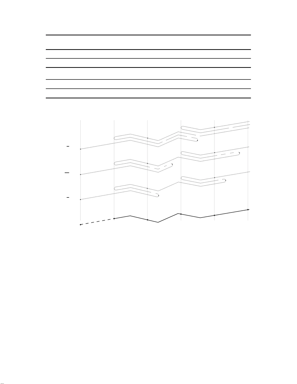
Sp eedup in the T ra v eling Repairman Problem wit h Unit Tim e Windo ws Greg N. F rederic kson Barry Wittman July 7, 2018 Abstract The input to the unro oted tra veling repairman problem is an undirected metric gra ph and a s ubset of no des, ea ch of which has a time window of unit leng th. Given that a repairma n can start at any lo cation, the goal is to plan a ro ute that visits as many no des as po ssible during their re s pective time windows. A p olynomial-time bicr iteria approximation algor ithm is prese nted for this problem, g aining an increas e d fraction of repairman vis its fo r increased sp eedup of repair man motion. F or s peedup s , we find a 6 γ / ( s + 1)-approximation for s in the range 1 ≤ s ≤ 2 and a 4 γ / s -approximation for s in the ra nge 2 ≤ s ≤ 4 , wher e γ = 1 on tree-shap ed net works and γ = 2 + ǫ on gener al metric graphs. 1 In tro duction When plann ing the route for an agen t w ho needs to dr op off supp lies, mak e repairs, deliv er imp or- tan t inf orm at ion, or other similar tasks, distance trav ele d ma y not b e the only imp ortan t metric. The usefulness of visiting a particular lo cation may b e hea vily d epend en t on time. Consider the example of a client wh o sc hedules a wind o w of time durin g which he or she w ill b e home. An appliance repairman will b e able to p erform repairs only d uring that time win d o w. In the last decade, the algorithms comm unity has ac hieve d muc h p r ogress with time-sensitiv e routing p roblems of this kind . These problems typical ly iden tify the lo cations to b e v isited and the cost of tra v eling b et w een th em as the n odes and edges, r espectiv ely , of a weigh ted, u n directed graph. F or example, th e orien teering problem [1, 2, 5 , 7, 9] seeks to find a path th at visits as man y no des as p ossible b efore a global time deadline. The deadline trav eling salesman pr oblem [2] generalizes this problem fu rther by allo wing eac h lo cation to hav e its own deadline. Th is problem can b e generalized ev en fu rther to the trav eling repairman problem [2 , 4, 8, 12, 16, 19] b y allo wing eac h lo cation to hav e a time windo w d u ring whic h it m ust b e visited to receiv e credit. In [12], we introdu ce d the fi r st p olynomial-time algorithms that giv e constant appro ximations to the tra v eling r ep airman problem with unit-time wind o ws when ever the un d erlying graph is a tree or a metric graph . In this v ersion of th e problem, a time wind o w is identified with eac h servic e r e quest whose lo cation is giv en by the no de with whic h it is asso ciat ed. Let a r epairman earn a sp ecified pr ofit for visiting a service request du ring its time window. A planned sequ ence of visits made by tra v eling at a giv en sp eed is called a servic e run . Th e goal of the tra ve ling repairman problem is to plan a service run that maximizes p rofit. Unlik e muc h of the preceding literature [2, 4 ], we considered th e unro oted ve rsion of th e problem, in which the repairman ma y start at any time from any lo catio n and stop similarly . Although the unr ooted problem is no hard er than the ro oted problem, w h ic h sp ecifies a starting p oint, it is a fascinating and difficult problem in its own righ t. Both p r oblems a re NP-hard w h en the graph is a tree [12] and APX-hard for a general metric graph [13]. 1 As a counterp oin t to the repairman problem, we also in tro duced the s p eedin g deliv eryman problem in [12, 13], with an alternativ e optimization paradigm, namely sp eedup . Th e input to the sp eeding deliv eryman pr oblem is the same as the inpu t to the tra ve ling repairman p roblem, but the goal is to find the min im um sp eed n ece ssary to visit al l service r equests dur ing their time windo ws and th us collect all profit. The deliv eryman problem is similarly hard, and in [12, 13] w e in tro duced p olynomial-time approximat ion algorithms for it. In b oth the repairman and delive rym an p roblems, o ur algorithms from [12, 13] rely on trimming windo ws so that the resulting time windows are pairw ise either identica l or non-ov erlapping. T o trim time w in do ws, we firs t mak e d ivisions in time eve ry . 5 time u nits, starting at time 0. W e call the time int erv al that starts at a particular division an d contin ues up to the next division a p erio d . Because w e allo w no wind o w to start on a p erio d b oundary , eac h time w indo w will completely o v erlap exactly one p erio d and partially o v erlap the tw o neighboring p erio ds. T rimming then remo v es those parts of eac h windo w that f all outside of the completely ov erlapp ed p erio d. This pro cess of trimming in curs a p enalt y in our approximati ons that is a reduction b y a factor of 1 / 3 in the num b er of requests serviced b y th e repairman and an incr ease b y a factor of 4 in the sp eedu p needed b y the d eliveryman. Y et one migh t exp ect that a sp ectrum of p erformance is p ossible b et wee n these tw o extremes. If we hav e any particular sp eedu p s greater than 1 but less than 4, w e exp ect an increase in the num b er of serviced requests, prop ortionate in some sense to s . Indeed, this is so, as w e show in this pap er. The concept of s p eedu p has b een used in the sc hedu lin g communit y since its in tro duction in [15]. S ubsequen t w ork in [18] refined th e tec hn ique an d ga v e it the name r esour c e augmentation as w ell as notation suitable for sc heduling. Results in [3] hav e made n ota ble strid es by pro ducing O (1)- sp eed O (1)-appro ximation algorithms for some kind s of scheduling problems. I n other words, b y increasing the sp eed of the mac hines on whic h the jobs are run by a constan t facto r, the resulting sc hedule can ac hiev e a measure of p erformance within a constan t factor of the optimal sc hedule run on machines at a baseline sp eed. Although w e do not u se the same tec hn iques or notation giv en in these pap ers, we note the connection b etw een sc hedu lin g and time-constrained routing and the v alue of resource augmentati on when fi nding approximati on algorithms for eac h class of p roblem. F or u n it-t ime win d o ws w e p resen t an algorithm th at finds app ro ximatio ns parameterized by sp eedup s and a factor γ , where γ = 1 for a tree and γ is no more than 2 + ǫ for a metric graph. These v alues for γ are explained in Sect. 2. F or s in the range 1 ≤ s ≤ 2, our algorithms fi nd a 6 γ / ( s + 1)-appro ximation. F or s in the range 2 ≤ s ≤ 4, our algorithms find a 4 γ /s -appro ximation. As long as un it sp eed is no greater than the sp eed needed for an optimal service r un to collect all p ossib le profit, ou r r esults will hold. W ere the unit sp eed considerab ly faster th an is needed to service all requests, the idea of offsetting the sub -optimal it y of an approximat ion by increasing sp eed b eyond that of an optimal r u n b ecomes meaningless. Our analysis dep ends up on the in teractions b et wee n sp eedup and trimmin g, bu t setting the starting p oint for p artiti oning p erio ds at time 0 as we d id in [12] may n ot result in the m ost profitable r un o v er tr im m ed windo ws. Esp ecially in the case of non-in teger sp eedups, careful stu dy suggests that some particular starting p oin t for p erio ds ma y b e better than others. If w e rep eatedly c ho ose different starting p oin ts, r un our repairman algorithm on trimmed windows, and alwa ys ke ep the b est answ er foun d so far, we can establish b etter b ounds on the fi nal appro ximation. Although there are an infinite num b er of p oint s to s ta rt partitioning p erio ds f rom, we can fi nd a c anonic al set of starting p oints that are representa tiv e of all p ossible starting p oin ts, and the size of th is set is linear in the num b er of service requests. Then, for eac h set of p erio ds we use, we tr im the windo ws and run a b asic repairman alg orithm. F or eac h set of trimmed windo ws, our analysis dep ends on an ensemble of runs, ea c h of whic h mo v es bac kw ard and f orw ard along the path of an optimal run. The ensemble is comp osed of a num b er 2 of runs tra v eling at a sp eedu p s faster than an optimal run trav els. While it is to o exp ensiv e to determine an actual optimal ru n unless P = NP, our analysis will r ely only on a defin iti on of eac h run in the ensem ble in terms of th e optimal run. On e run in the ensem ble might b e effectiv e in servicing requests s er v iced b y an optimal run ve ry early in th eir resp ectiv e win do ws. Another run migh t b e effectiv e in servicing requests serviced by an optimal run ve ry late in their r esp ec tive windo ws. T ogether, th ese r uns would service every request on trimmed wind o ws that an optimal run would service on untrimmed windows. An optimal r un on trimmed win d o ws, then, wo uld ac hiev e at least the a verag e service of the ensemble of run s taken as a whole. Lik ewise, the b est run from among all p ossible choice s of trimming wo uld ac hiev e at least the a verag e service tak en o v er all runs in the ensemble. Except for th e factor of γ that do es not come from trimming, our algorithm find s a ru n whic h p erforms as w ell as this a verag e. O ur analysis of an ensemble guaran tees that a certain f racti on of p rofit is alw a ys collec ted by the run p rod uced by our algorithm. Again, w e know the en s em ble of run s only symbolically , b ecause we cannot efficien tly kno w th e ins tantiat ion of th ese ru ns unless P = NP. The c hallenge has b een to devise ensem bles s o th at our analysis w ill establish a go o d p erformance f or our algorithm. Although w e are the firs t to extend time window problems into the realm of sp eedup, muc h other related w ork is b eing done with time w in do ws. F or general metric spaces and general time windo ws together in the ro oted problem, an O (log 2 n )-appro ximation is giv en in [2 ]. An O (log L )- appro ximation is give n in [6], for the case that all time wind o w s ta rt and end times are in tegers, where L is the length of the longest time wind o w. In constr ast, a constan t ap p ro ximation is giv en in [8], but only when there are a constan t num b er of differen t time wind o ws. F ollo wing the initial publication of our work in [12], an extension was giv en in [6] that giv es an O (log D )-a pp ro ximation to the un rooted problem w ith general time win do ws, where D is the ratio of the length of largest time windo w to the length of the smallest. P olylogarithmic appro ximation algorithms to the directed tra v eling salesman problem with time windows ha v e b een giv en in [7] and [17]. The repairman problem w ith time windows has also b een studied in the op erations researc h comm un it y , as in [10] and [11], where it is exhau s tiv ely solv ed to optimalit y . Note that the b icrite ria appr o ximatio n that we give will guaran tee the r epairman a greater fraction of th e optimal profit by sp eeding up beyond the sp eed of the optimal s er v ice ru n. Although w e are the fir st to iden tify tec hniques that allo w for a trade-off b etw een requests serv iced and sp eedup, th ere are other b icrite ria appro ximations for rep ai rm an problems. F or example, a bicriteria appro ximation is presente d in [2] that allo ws the repairman to serv ice more requests if the time windo ws are all lengthened b y some amoun t ǫ . If the time window for request s i starts at time t and ends at time t ′ , this lengthening w ould c hange eac h time window from [ t, t ′ ) to [ t, (1 + ǫ ) t ′ ). In contrast, the effect of run ning at sp eedu p s is equiv alen t to in creasing all times by some factor, c hanging time win d o w [ t, t ′ ) to [ st, st ′ ). Before we explain our bicriteria algorithms in depth, w e will summ arize in Sect. 2 our results from [12] as we ll as r ece nt improv emen ts. In Sect. 3, we will explain th e basic mec hanisms n ee ded for the av eragi ng analysis u sed in our ensem ble app roac h. In Sect. 4, we will int ro duce the concept of canonical sets needed to mak e our algorithms practical for arb itrary v alues of sp eedup s . In Sect. 5, we will giv e the analysis that p ro v es our app ro ximation results for s p eedu p s in th e range 2 ≤ s ≤ 4. Finally , in Sect. 6, we will give the more in v olv ed an alysis pro ving approxi mation results for sp eedup s in the range 1 ≤ s ≤ 2. 3 2 Algorithms for Repairman without Sp eedup W e contin ue to restrict our fo cus to the tra v eling repairman p roblem with u nit-time win do ws. F or this p roblem, our repairman appro ximation algorithms in [12, 13] trim the time w indo ws so that the r esulting wind o ws can b e p artiti oned into n on -ov erlapping p eriod s. T hese algorithms ident ify a v ariet y of go od paths within eac h separate p erio d and then use dynamic p rogramming to s elect and p aste th ese paths together into a v ariet y of longer go o d paths an d ultimately a goo d service run for the wh ole problem. Optimal paths within eac h p erio d can b e f ound in p olynomial time when the underlyin g graph is a tree, but only app ro ximately optimal paths are found on a metric graph. T o unify the notation b et wee n th ese approac hes, we describ e the approxima tion factor for finding paths with in eac h p erio d u sing γ , wh ere γ = 1 for a tree and γ = 2 + ǫ f or a metric graph. Results from [12] clearly show that γ ≤ 5 for a metric graph , b ut this result has b een impro ve d to 2 + ǫ b ecause of results in [7]. T o d escrib e th e run ning time for these repairman algorithms we b ound the time by Γ( n ), where Γ( n ) is O ( n 4 ) for a tree and O ( n O (1 / ǫ 2 ) ) for a metric graph, w here the tree b ound comes fr om r esults in [12] and the metric graph b ound can b e derive d by augmenting those results with tec hniques from [7]. A fu ll explanation of this imp r o v ed result is av ailable in [13]. 3 The Ensem ble Approac h for Analyzing P erformance The t wo results cited ab o v e giv e analysis for ru n s afte r trimming for the cases of no sp eedup ( s = 1 guaran teeing 1 / (3 γ ) of optimal profit) and fu ll sp eedup ( s = 4 guaran teeing 1 /γ of optimal profit ac hiev ed at the original sp eed). O ur analysis cann ot examine sp eeds lo w er than the r eference sp eed of 1 (i.e, slo wdown) b ecause there is no guarantee that a slow er run can ev er earn an y constan t fraction of the pr ofit of a faster ru n . Lik ewise, ab o v e a sp eedup of 4, the effects of trimming are completely offset. Th us, this range of sp eedups is the only range for whic h our bicriteria an alysis seems practical. F or this range 1 < s < 4, our analysis uses a n umb er of differen t s er v ice run s that are defined by mo ving b ac kw ard and forward along an optimal tour R ∗ . W e rely on a verag ing ov er a suitable ensemble of ru ns to establish that th e run R generated b y our algorithm d oes wel l. Let R ∗ b e an optimal service run at unit sp eed originally starting at time 0. In defining the service run s that we use in our an alysis, we use the term r acing to d escrib e mo v emen t, f orw ard and bac kw ard, along R ∗ at a sp eedup of s times the sp eed at wh ic h R ∗ tra v els. Please refer to Figure 1 for an example of runs racing at s = 2. F or conv enience, let δ = 1 / (2 s ), which is the time needed to tra v el at sp eed s the distance trav ele d in one p erio d at unit sp eed. One of the runs o ver w hic h we a verag e is serv ice run A , defined as follo ws. Start r un A at time 0 at the lo cati on that R ∗ has at time − . 5. Th en run A follo ws a pattern of racing forwa rd along R ∗ for 1 p erio d, racing bac kward along R ∗ for 1 − 2 δ p erio ds, and then racing forw ard along R ∗ for 2 δ p erio ds. The p ositions reac hed by r un A at the times 0, . 5, 1, 1 . 5, and 2 are ind ica ted in Figure 1. Note th at the p att ern of mo v emen t for r u n A rep eats ev ery 2 p erio ds. Define A R , the “ r e v erse ” of A , as follo ws. Start run A R at time 0 at the lo cation that R ∗ has at time . 5. Then run A R follo ws a rep eating pattern of racing forw ard along R ∗ for 2 δ p erio ds, racing bac kw ard along R ∗ for 1 − 2 δ p erio ds, and then r ac ing forward along R ∗ for 1 p erio d. Similarly , the p ositions reac hed by run A R at times 0, . 5, 1, 1 . 5, and 2 are indicated in the same fi gure. If a ser v ice request p is serviced by a run R dur ing the p erio d that the time w indo w of p has b een trimmed int o, w e sa y that R c overs p . W e partition the set of requests wh ose windows are trimmed in to a giv en p erio d into th r ee sets: Set T con tains those requests serviced by R ∗ in that same p erio d, set E co ntains those requ ests serviced by R ∗ in the preceding p erio d, and set L 4 con tains those requ ests serviced b y R ∗ in the follo wing p erio d. S ee Fig ure 1 for an example: Ru n A services requests in L for eac h p erio d, and it services requests in T for ev ery second p erio d. Note, for example, that requests serviced on R ∗ b et w een times 0 and . 5 are serv iced b y A durin g th at same p erio d. Run A R Optimal Run R ∗ Run A L T L L T L L E T E E T 0 . 5 1 1 . 5 − . 5 2 0 . 5 1 1 . 5 2 0 . 5 1 1 . 5 Figure 1: Runs A and A R with a sp eedup of 2 based on an optimal ru n. The pattern in A R p erfectly complemen ts A to giv e full co v erage. T imes are lab eled on the optimal ru n as we ll as runs A and A R . Segments of eac h run are also d esig nated L , T , and E dep end in g on whic h subs et of runs they add cov erag e to. Th e ligh t vertic al lines indicate sh ared p ositions on the run s, not id en tical times. W e n umb er the p erio ds − 1, 0, 1, 2, an d s o on b y th e in teger m ultiples of . 5 that giv e their starting times. The lab els L , T , and E in Figure 1 mak e it clear that every p erio d num b ered 1 and later has full co v erage. The combinatio n of run s A and A R ensures that the lo cati on of a giv en request is visited three times: d uring the same p erio d, the p revious p erio d, and the f ollo wing p erio d that the request w as visited b y R ∗ . Thus, we guarante e that our com bination of ru n s visits the request no matter wh ic h per io d its wind ow was trimmed in to. Ho w ev er, it app ears that p erio ds − 1 and 0 only hav e partial co v erage. This app aren t discrepan cy is an endp oint anomaly . In fact, p erio d − 1 n ee ds no co v erage b ecause no locations visited b y R ∗ are visited in this p erio d . Likewise, there are no requests in set E serv iced b y R ∗ during p erio d 0 b ecause suc h requests would ha v e b een trim m ed into p erio d − 1, w h ic h is imp ossible. Although there migh t b e some sup erficial r esem blance b et we en the L , T , and E sets and the small margin and large margin cases discussed in [2], the approac h in that pap er iterativ ely run s sp ecialize d algorithms that progressive ly redefin e the meaning of small margins and large margins. In con trast, th e thr ee sets that we use are fixed for an y giv en trimming sc heme, d o n ot ha v e separate algorithms tailored for eac h one, and are used p urely for accoun ting. Let S b e a su bset of service requests. Define the c over age of S b y a run R , wr itt en cov er R ( S ), to b e the num b er of r equests in S satisfied by R divided by the total num b er of requests in S . Define the co v erage of S by a set U of r uns, w ritten cov er U ( S ), to b e the a v erage of cov er R ( S ) for ev ery ru n R ∈ U . Prop osition 3.1 ( Av erage Co verage) L et { S 1 , S 2 , S 3 , ...S a } b e a c ol le ction of sets of servic e r e quests such that S i S i gives al l the r e quests servic e d by R ∗ on untrimme d windows. L et U b e a set of servic e runs. If min i { cov er U ( S i ) } = µ , then ther e is at le ast one servic e run ˆ R ∈ U suc h that pr ofit ( ˆ R ) ≥ µ · pr ofit ( R ∗ ) . The Av erage Co ve rage Prop osition formalizes the follo wing intuition. Let a group of service runs ac hiev e s ome co v erage ov er a set of r equests. Let u s also sa y that we hav e divided those 5 requests into many d ifferen t su bsets, some of whic h may o ve rlap, but the union of all th e subsets is the original set of requests. If we tak e the subset of r equests with the worst av erag e co ve rage, some service run in the group co v ers a fraction of total requests n o smaller than that w orst a v erage co v erage. Otherwise, the a v erage co v erage of all su bsets wo uld b e worse than th e co v erage of the w orst co vered subset, which is a cont radiction. Giv en a w a y of dividing r equests in to subsets, we wish to prov e that some set of service run s ac hiev es a particular lo we r b ound on a v erage cov erag e. F or the case of un it- length time windows, w e d ivide r equests in to subsets b ased on memb er s hip in L , T , or E sets (or smaller partitions of these three sets). Since our dynamic programming ap p roac h find s an optimal ru n on trimmed windo ws, to within a factor of γ , w e kn ow that this run m ust p erform at least as we ll as the b ound w e pr o v e. F or analyzing s = 2 and s = 3, we u se ensem bles of runs . W e a verag e the co v erage ov er sets L , T , and E b y summ ing the low est cov erag e for the requests in eac h set and dividing by the total n umb er of run s used. By the Averag e Co ve rage Prop osition, this a v erage giv es a lo w er b oun d on the p erformance of an optimal run on trimm ed in terv als. Theorem 3.1 R unning a r ep airman algorithm fr om [ 12] at a sp e e dup of s = 2 gives a 2 γ -appr oximation to r ep airman with unit- time windows in Γ( n ) time. Pr o of: T o analyze the p erformance of th e resulting service run , we consider run s A and A R , as defined ab o v e. Refer to Figure 1 f or an example. Run A co v ers all of the requests in set L and all of the requests in s et T whic h fall in eve n num b ered p erio ds with r esp ect to R ∗ . Run A R co v ers all of the requests in set E and all of the requests in set T whic h fall in o dd n umb ered p erio ds. F or eac h ru n, we record a 1 in eac h set for ev ery p erio d whic h is completed co ve red. Note th at L even is that subs et of requ ests in set L th at w ere serviced by R ∗ in ev en num b ered p erio d s and L o dd is that subset of requests in set L that we re serviced by R ∗ in o dd num b ered p erio ds, and similarly for T and E . W e su m these con tributions into yields and then divide the yields b y the total num b er of run s to get the av erage co v erage for designation. T able 1 illustrates this pro cess, in wh ic h w e get an a ve rage co v erage of 1/2. Let ˆ R b e th e service run p r odu ced by th e app ropriate repairman algorithm from [12]. By the Av erage Co ve rage Pr oposition, pr ofit ( ˆ R ) ≥ max { pr o fit ( A ), pr ofit ( A R ) } ≥ (1 / 2 ) pr ofit ( R ∗ ) /γ , giving a 2 γ -appro ximation. ✷ L even L o dd T even T o dd E even E o dd Run A 1 1 1 0 0 0 Run A R 0 0 0 1 1 1 Yield 1 1 1 1 1 1 Av erage Cov erag e 1/2 1/2 1/2 1/2 1/2 1/2 T able 1: Av eraging of runs A and A R with sp eedup s = 2. Theorem 3.2 R unning a r ep airman algorith m fr om [12] at a sp e e dup of s = 3 finds a 4 γ / 3 - appr oximation to r ep airman with unit-time windows in Γ( n ) time. Pr o of: T o analyze the p erformance, we use four run s: A , A R , ~ A , and ~ A R , where ~ A and ~ A R are shifted versions of A and A R . Run ~ A f oll o ws the same pattern as A but starts th e p attern at time 6 1 / 2 at the lo catio n R ∗ has at time 0. Run ~ A R follo ws the same pattern as A R but starts the p attern at time 1 / 2 at the lo cat ion R ∗ has at time 1. Ru n A , no w run ning with sp eedup s = 3, co v ers all of the requests in L and T b ut only half the requests in E . Run A R co v ers all of the r equests in T and E bu t only half the requests in L . T he shifted runs are copies of A and A R , co v ering all of T and the other half of the requests of E and L , resp ectiv ely . As b efore, we sum the con tribu tio ns and divide b y the total n umb er of runs to fin d the a v erage co v erages shown in T able 2. T h e w orst co ve rage for an y set, av erage d ov er ru ns A , A R , ~ A , an d ~ A R , is 3/4, corresp onding to sets L and E . Let ˆ R b e the service ru n p rod uced by the appropriate r epairman algorithm fr om [12]. By the Av erage Co v erage Prop osition, pr ofit ( ˆ R ) ≥ max { pr ofit ( A ), pr ofit ( A R ), pr ofit ( ~ A ), pr ofit ( ~ A R ) } ≥ (3 / 4) pr ofit ( R ∗ ) /γ , giving a 4 γ / 3-approxi mation. ✷ L even L o dd T even T o dd E even E o dd Run A 1 1 1 1 1 0 Run ~ A 1 1 1 1 0 1 Run A R 0 1 1 1 1 1 Run ~ A R 1 0 1 1 1 1 Yield 3 3 4 4 3 3 Av erage Cov erag e 3/4 3/4 1 1 3/4 3/4 T able 2: Av eraging of r u ns A , ~ A , A R , and ~ A R with sp eedup s = 3. 4 Canonical Collections and Their Use in Algorithms If sp eedup is a rational num b er, let s = q /r , wh er e q an d r are r ela tiv ely prime. Otherwise, if the sp eedup is an irr atio nal n umb er, we assum e r to b e infi nite. Let m b e the num b er of requests. Belo w w e will define algorithm SPEE DUP suc h that it runs a repairman algorithm on eac h set of p erio ds fr om among a collection of min { r , m } different sets of p erio ds. If s is rational and r ≤ m , w e create sets of p erio ds starting at r time instants sp read u niformly fr om time 0 up to time 1 / 2. If any window wo uld start on any p erio d or half p erio d b oundary , we sh ift th e p erio ds by a small amoun t to av oid this case. When r > m , SPEE DUP will use a canonical coll ection of sets of p eriods whic h is equally as effectiv e as the r sets (whenever r is finite) but has size just linear in m . The pro cedure CANONICAL defined b elo w “norm alizes” the b eginnings of all the time windows in to the range (0 , 1 / 2) and then pic ks a time b etw een eac h consecutiv e pair of b eginnings to b e the starting p oin t for a new set of p erio ds. Lemma 4.1 Any given set of p erio ds is e quivalent to one of the at most m sets of p erio d s in the c ano nic al c ol le ction, and this c ol le ction c an b e identifie d in O ( m log m ) time. Pr o of: Without loss of generalit y , w e assume that al l time win d o ws ha ve unique starting times after normalization. Lab el the norm ali zed starting times of the w in do ws h 1 , h 2 , h 3 , . . . , h m in ascending order as pro duced by the pro cedure CANONIC AL. The first p oin t c hosen by CANONICAL is 0. The second p oin t c hosen is ( h 1 + h 2 ) / 2, the third is ( h 2 + h 3 ) / 2, and so on. A starting p oin t uniquely d ete rmin es a s et of p erio ds, with eac h s uccessiv e p erio d starting at .5 time un its after the start of the previous one. Eac h set of p erio ds induces a trimming of time 7 CANONIC AL F or time window s i , Let t ( s i ) b e the s ta rting time of s i . Let a b e th e largest inte ger suc h that a/ 2 < t ( s i ). Set h i to b e t ( s i ) − a/ 2. Sort the h i v alues, relab eling them h 1 , h 2 , . . . , h m in increasing order. Let the first set of p erio ds start at time 0. F or i from 2 to m , Let the i th set of p erio ds start at time ( h i − 1 + h i ) / 2. windo ws according to the trimming pr o cedure give n b efore. Defin e an equiv alence relation on sets of p erio ds: Consid er t w o trimmings ind uced by tw o different sets of p erio ds. If the difference in starting times from one set of p erio ds to the n ext is the same for all time windo ws, th en those t wo sets are equiv a lent. Consider the time window starting at h i . Those sets of p erio ds are equ iv alen t that hav e starting times s tr ict ly b et ween h i and h i +1 . Only by mo ving the starting time earlier than h i will the tr im m ing of the earlier windo w (starting at h i ) c hange, and only by mo ving the starting time later than h i +1 will the trimming of the later windo w (starting at h i +1 ) c hange. Because our formulat ion of the trav eling repairman pr oblem do es not sp ecify a starting p osition or time, all equiv alen t sets of p eriod s are functionally iden tical. This equiv a lence relation p artiti ons all p ossible sets of p erio ds in to equiv al ence classes. By choosing a representati ve fr om eac h of these m equiv ale nce classes, we find a collection of m sets of p erio ds that co vers all p ossible trimmings. The r unning time for C ANONIC AL is O ( m log m ) b ecause the m starting times are sorted and all other wo rk is linear. ✷ With CANONIC AL d efined, the description of SP EEDUP using sp eedup s is straigh tforwa rd. W e assume that no w in do w starts on a p erio d b oundary as this situation can b e easily remedied. Let REP AIR b e a b asic repairman algorithm ru n after the trimming pr ocess has tak en place, suc h as th e algorithms in [12 ]. As s h o wn in [12], RE P AIR on a tr immed instance h as an appr oximati on ratio of at most γ and a runnin g time of Γ( n ). SPEEDUP If s is rational and s = q /r in reduced form, w h ere r < m , F or i from 1 to r , Let h i b e ( i − 1) /r . Otherwise, Let h 1 , h 2 , h 3 , . . . h m b e the p erio d starting times foun d b y CANONICAL. (Note that the total num b er of h i v alues is min { r, m } .) F or i from 1 to min { r , m } , Start a set of p erio ds at time h i and trim eac h wind o w into the p erio d it completely fills. Run REP AIR on the trimmed wind o ws and r eta in the b est resu lt so far. Since algorithm SPEEDUP runs REP AIR a tota l of m in { r, m } times, the runn ing time for SPEEDUP is O (min { r , m } Γ( n )). 8 Observ at ion 4.1 Algorithm SPEEDUP works for any r e al numb er 1 ≤ s ≤ 4 ; however, our analysis wil l assume that s is a r ational numb er such that s = q /r . In the c ase that s is irr ational, our analysis stil l holds b e c ause the fu nc tions of s with which we b ound p erform anc e ar e pie c ewise smo oth and c ontinuous. Thus, we c an cho ose r at ional numb ers arbitr a rily close to any r e al numb er, and our analysis wil l b e wel l-b ehave d in the limit. 5 Analysis of Sp eedup in the Range 2 ≤ s ≤ 4 In this section, w e describ e an ensemble of r uns and the cov erag e giv en b y suc h a set of r uns when sp eedups s is in the r an ge 2 ≤ s ≤ 4. Based on the a verag e cov erag e of th e ensem ble, the algorithm SPEEDUP pro duces a 4 γ /s -approximati on in this sp eedup range. W e assume that no time win do w s tarts at time i/ (2 r ) for an y integ er i . If any d o, we can p erturb all times sligh tly so that this is not th e case. Let [ w , w + 1) b e any time window. Let ω b e th e smallest int eger m ultiple of 1 / (2 r ) that is greater than w . W e d esignat e subinterv als [ w , ω ), [ ω , ω + 1 / (2 r )), [ ω + 1 / (2 r ) , ω + 2 / (2 r )), . . . , [ ω + (2 r − 1) / (2 r ) , w + 1) by w 0 , w 1 , w 2 , . . . , w 2 r . When a giv en time windo w is trimmed, some p ortion of the original w in do w w ill lie in an earlier p erio d, half of it in the p erio d it w as trimmed in to, and the remaining p ortion in the follo wing p erio d. As b efore, the goal is to u se an ensemble of run s to co v er ev ery p art of eac h time windo w so that we can show a lo w er b ound on p rofit with an av erag ing argum en t. Ho w ev er, using sets L , T , and E alone is too coarse-grained for general s . Instead, w e r ec ord the co ve rage of eac h sub in terv al w i . F or accoun ting pur p oses, we assign a 1 for any subinte rv al whic h is co v ered ev ery p erio d, a 1 / 2 for an y sub in terv al co v ered ev ery other p erio d, an d a 0 otherwise. This accounti ng sc heme implicitly a v erages r uns A and A R with their r espective shifted v ersions ~ A and ~ A R . Be cause the u nion of requests serviced dur ing these subinte rv als consists of all the requests serviced by an optimal p ath, the Av erage C o v erage Prop osition still applies. W e p artiti on sets L , T , and E in to sub sets: L 1 through L r , T 1 through T r , and E 1 through E r resp ectiv ely . If w e partition eac h p erio d into r equal-length divisions, then su bset L j , T j , or E j , for an y give n j , will consist of those service requ ests fr om set L , T , or E , resp ectiv ely , whic h we re serviced by the optimal run in the j th division of a p erio d. Note that, for a giv en p eriod starting time, the wind ow for a service r equ est can only ov erlap w ith 2 r + 1 of these divisions. Th us, w e can mak e a one-to-one mapping of th e 2 r + 1 sub in terv als of a windo w to 2 r + 1 of the 3 r s ubsets of L , T , or E . F or a given window, some s et of p erio ds m ap s all subinterv als of the wind o w to L 1 through L r , T 1 through T r , and E 1 . Another set of p erio ds maps all subinterv als of the windo w to L 2 through L r , T 1 through T r , and E 1 through E 2 . Eac h remaining set of p erio ds maps one fewer L i subset and one additional E j subset, w h ere j = i + 1 for set i . T able 3 sh o ws whic h su bsets are mapp ed to su bin terv als of some time w indo w d epen ding on the s et of p erio ds used. Figure 2 giv es th ree examples of t yp e A runs for v arious sp eedup s in the range 2 < s < 4. Note that all of the r u ns in this figure arr ive at the same p osition at the b eginning of ev ery second p erio d, namely at times 0 , 1 , 2 , and so on. P ortions of run s servicing requests in L , T , and E or v arious subsets are identi fied: subset E 1 b eing those service r equests of E serviced b y R ∗ in the first half of a p erio d for s = 7 / 2, sub sets T 1 , T 2 , T 3 , E 1 , E 2 , and E 3 b eing those service requests of T or E serviced by R ∗ in v ario us quarter p erio ds for s = 11 / 4, and s ubsets T 1 , T 2 , E 1 , and E 2 b eing those service requests of T or E serviced by R ∗ in v arious th irds of p erio ds f or s = 7 / 3. Algorithm SP E EDUP run s a repairman algorithm on min { r, m } different sets of p erio ds and tak es the b est run from those choice s. Theorem 5.1 F or any s in the r ange 2 ≤ s ≤ 4 , SP EEDUP finds a 4 γ /s -appr oximation to r ep airman with u nit-time windows in O (min { r , m } Γ( n )) time. 9 Set of Subinterv als P erio ds w 0 w 1 w 2 . . . w r w r +1 w r +2 . . . w 2 r − 2 w 2 r − 1 w 2 r 0 L 1 L 2 L 3 . . . T 1 T 2 T 3 . . . T r − 1 T r E 1 1 L 2 L 3 L 4 . . . T 2 T 3 T 4 . . . T r E 1 E 2 . . . . . . . . . . . . . . . . . . . . . . . . . . . . . . r − 2 L r − 1 L r T 1 . . . T r − 1 T r E 1 . . . E r − 3 E r − 2 E r − 1 r − 1 L r T 1 T 2 . . . T r E 1 E 2 . . . E r − 2 E r − 1 E r T able 3: Po ssible wa ys to map the su bin terv als of a time w indo w to subsets. Run A for s = 7 2 Run A for s = 11 4 Run A for s = 7 3 Optimal Run R ∗ 0 . 5 1 1 . 5 − . 5 2 0 . 5 1 1 . 5 2 0 . 5 1 1 . 5 2 0 . 5 1 2 L T E 1 T 1 L L T E 1 T 1 L L L T E 1 E 2 E 3 T 1 T 2 T 3 L L T E 1 E 2 E 3 T 1 T 2 T 3 L L L T E T L L E 1 E T L T L Figure 2: E xamples of t yp e A run s for three different sp eedups in the range 2 < s < 4, namely at 7 / 3, 11 / 4, and 7 / 2. Pr o of: F or an y win do w [ w , w + 1), on serv ice r un A , if a trimmed int erv al starts with sub in terv al w i , where 1 ≤ i ≤ r , then the windo w’s first q − 2 r + i subinterv als will b e co v ered eac h p erio d, and the n ext r su b in terv als after that will b e co v ered every other p erio d (but no f urther th an the last subinterv al). When s < 3, r un A completely co v ers sub sets L 1 through L r , co ve rs those requests in subsets T 1 through T r serviced b y R ∗ in h alf of the p erio ds, and co v ers those requests in sub sets T 1 through T q − 2 r and subsets E 1 through E q − 2 r serviced by R ∗ in the other half of the p erio ds. When s > 3, ru n A completely co vers su b sets L 1 through L r and subsets T 1 through T r , co v ers those r equests in sub sets E 1 through E q − 3 r serviced by R ∗ in half of the p erio ds, and cov ers those requests in su b sets E 1 through E r serviced b y R ∗ in the other half of the p erio ds. A similar analysis applies to ~ A , A R , and ~ A R . W e assign a 1 for any sub in terv al wh ic h is co vered ev ery p erio d and a 1 / 2 f or any su bin terv al co v ered ev ery other p erio d. F or runs A and ~ A together, w i earns a 1 for all r sets of p erio ds wh ere 0 ≤ i ≤ q − 2 r , giving a total of r for eac h suc h i . F or eac h i > q − 2 r , the total decreases by 1 / 2 from the total for i − 1. F or r uns A R and ~ A R together, w i gets 1 for all r sets of p eriod s where 10 2 r − ( q − 2 r ) ≤ i ≤ 2 r , giving a total of r for eac h suc h i . F or eac h i < 2 r − ( q − 2 r ), the total decreases b y 1 / 2 f r om the total f or i + 1. No w, w e tak e the total o v er all sets of p erio ds for b oth runs . F or ru ns A and ~ A together w e get a total of r for w 0 . F or r uns A R and ~ A R together w e get a total of r − (1 / 2) (2 r − ( q − 2 r )) = q / 2 − r . Summing these together, w e get a yield of q / 2 for w 0 . By symmetry , th e total for w 2 r is also q / 2. In the case that s < 3, th e con tribu tio ns for r uns A and ~ A together decrease by no more th an 1 / 2 as the cont rib u tions for runs A R and ~ A R together increase by 1 / 2 for eac h increment of i in the range 0 < i ≤ r . In th e case that s ≥ 3, contributions fr om A and ~ A together are constan t and contributions from A R and ~ A R together only in crease or sta y constan t for 0 < i ≤ r . Th us, the yield for all other w i in all cases is at least q / 2. S in ce r sets of p erio ds for the tw o pairs of ru ns cost a total of 2 r sets of p erio ds to a v erage o ve r, the yield for th e algorithm is at least q / 2 · 1 / (2 r ) = q / (4 r ) = s/ 4. Multiplying th e recipr o cal by γ giv es a 4 γ /s -appro ximation. By Observ ation 4.1, this result holds for all real v alues of s . Note that the d et ails of this p roof can also b e generated u sing the CR E A TE-T ABLE pro cedure giv en in Sect. 6. ✷ 6 Analysis of Sp eedup in the Range 1 ≤ s ≤ 2 A different analysis giv es us b etter p erformance as a fun cti on of s in the range 1 ≤ s ≤ 2. Based on the a verag e co v erage of the ensemble, the algorithm SPEEDUP pro duces a 6 γ / ( s + 1)-appro ximation in this s p eedu p range. W e consider fou r runs (and their shifts) and b ala nce their relativ e w eigh tings. F or the range 1 ≤ s ≤ 2, w e represent s p eedu p s as s = ( r + k ) /r with in tegers r ≥ 1 and 0 ≤ k ≤ r . Our analysis w ill r equire sev eral v ersions of A that h a v e different starting p oin ts. T o simplify notation, let a hop b e the distance tra vel ed in time 1 / (2 r ) at unit sp eed. L et A ∆ b e run A starting ∆ hops fu rther along and run A R ∆ b e r un A R starting ∆ hops fu rther bac k. Run A ∆ follo ws the same pattern of mo v emen t as ru n A but starts at t = 0 at the lo cat ion that R ∗ has at t = − 1 / 2 + ∆ / (2 r ). Its reverse A R ∆ follo ws the same pattern of mov emen t as A R but starts at t = 0 at the lo cation that R ∗ has at t = 1 / 2 − ∆ / (2 r ). Examples of run s A , A R , A r − k , and A R r − k are sho wn in Figure 3 f or s = 5 / 4 wh ere r = 4 and k = 1. P ortions of runs servicing requests in L , T , and E or v arious su bsets are id en tified: subsets L 4 , T 1 , T 2 , T 3 , T 4 , and E 1 b eing those service requests of L , T , and E serviced b y R ∗ in v arious quarter p erio ds. W e also define ~ A , ~ A R , ~ A r − k , and ~ A R r − k as in dicat ed earlier and implicitly av erag e the con tribu tions of these shifted runs w ith the con tributions of their uns hifted versions in T ables 5 and 6. In order to crea te these tables, we defin e a pro cedure called CRE A TE-T ABLE th at describ es the pro cess of d ete rmin ing cov erag e for a particular sp eedup s for a particular run mo v ed ∆ hops. Note that CREA TE-T ABLE is not an algorithm that is run in the pr o cess of finding an ap p ro ximation to a repairman problem w ith sp eedup. Rather, it p ro vides a template that can b e used to pro duce the tables used in analyzing the p erform ance of such approximati ons. Before CREA TE-T ABLE can b e completely d efined, it is necessary to explain the pattern of co v erage generated by a ru n. F or all t yp e A runs, this pattern tak es one of t w o forms. Let s b e a r ati onal num b er suc h th at s = q /r . T yp e A run s rep eat ev ery t w o p erio ds and thus can b e represent ed w ith a p attern of co ve rage that uses a 1 to signify a subinterv al co ve red every p erio d and a 1/2 to signify a sub in terv al co v ered ev ery other p erio d. Observe the mo v emen t of type A ru ns, n oti ng that su c h a run mo ves f orw ard in one p erio d the same d istance that run R ∗ mo v es in q subinterv als. During the next p erio d of time, a type A run mov es bac kw ard the same d istance th at run R ∗ mo v es du ring q − r sub in terv als and then forw ard the same distance that ru n R ∗ mo v es du ring r subinterv als. Then, the pattern rep eats. 11 Run A Run A R Run A r − k Run A R r − k Optimal Run R ∗ − . 5 0 . 5 1 1 . 5 2 0 . 5 1 1 . 5 0 . 5 1 1 . 5 2 0 . 5 1 0 . 5 1 1 . 5 2 T 2 T 3 T 4 E 1 T E 1 T 2 T 3 T 4 E 1 T L 4 T L 4 T 1 T 2 T 3 L 4 T L 4 T 1 T 2 T 3 L 4 E T 4 E E L T 1 L L T 1 L L Figure 3: Examples of r uns A , A R , A r − k , and A R r − k with a sp eedup of s = ( r + k ) /r = 5 / 4. When s < 2, ru n A d uring its first p erio d in the pattern co v ers q successiv e subinterv als as it mo v es forward, while in its second p erio d cov ers r su bin terv al s as it mov es forward. Note that those subinterv als co v ered as A mo v es bac kw ard add nothing add itio nal to the co v erage. Thus, this pattern of co v erage is repr esen ted as r rep etitio ns of 1 and q − r r epetitions of 1/2. CREA TE-T ABLE( hops ∆ ) Let the first elemen t of the co v erage pattern b e in dexed at 0. Let the subinterv als of interest b e num b ered 0 through 2 r . Define function C based on the co v erage p att ern, suc h that: C ( i ) =    1 if term i of the pattern is 1 1 / 2 if term i of the pattern is 1/2 0 otherwise Define function F on in tegers i , where 0 ≤ i ≤ 2 r : F ( i ) = P r − 1 j =0 C ( i + j − ∆). Define function F R on the same domain: F R ( i ) = F (2 r − i ). The final co v erage function defined by th e table is giv en by F ( i ) + F R ( i ). CREA TE-T ABLE defines f unctions F ( i ) and F ( i ) R suc h that the fin al co v erage that we define is F ( i ) + F ( i ) R for i = 0 , 1 , . . . , 2 r . Note that the functions F and F R are p iece wise linear func- tions with r anges dep end en t on th e fu ndamen tal pattern of cov erag e. Due to its constru ctio n, the com bination F ( i ) + F R ( i ) is also a piecewise linear fu nctio n and symm etrical. Thus, only the range 0 ≤ i ≤ r n eed b e listed in tables. Although CRE A TE-T ABLE giv es a pr o cedure for creating a table for a giv en sp eedup, we need 12 tables expressed sym b olically to p ro v e co v erage for a range of s p eedu ps. Ins te ad of using sp ecific n umb ers, we can lea ve the b asic p at terns of subinte rv al co v erage for a giv en st yle of run (suc h as t yp e A ru ns) with its shifted version in terms of q and r . B y shifting this pattern r times and summing the r esults together, w e account for the differen t alignments a time window might ha ve with resp ect to th e v arious su bin terv al s. This su m is the function F , wh ic h we can no w expr ess as a piecewise linear fun ctio n p aramet erized by q and r . F unction F R , whic h describ es type A R runs, can b e similarly describ ed. T o com bine the tw o fun ctio ns symbolically , w e sort the end p oint s of the subinte rv al ranges from b oth descriptions together. If, for the giv en range of s p eedu ps b eing considered, there are tw o end p oints wh ic h cann ot b e ordered, w e su bd ivide the r ange of sp eeds so that, in eac h n ew sp eed r ange , the t wo end p oints in question can b e ordered. Once the end p oin ts of eac h subinterv al range ha ve b een sorted, com bining the descriptions from the normal and rev ersed f unctions of the r uns is ac hiev ed by simply sum m ing eac h range. F ( i ) =      r − 1 2 i r + 1 2 k − i 1 2 r + 1 2 k − 1 2 i 0 ≤ i ≤ k k ≤ i ≤ r r ≤ i ≤ r + k F R ( i ) =      1 2 i − 1 2 r + 1 2 k 1 2 k − r + i 1 2 i r − k ≤ i ≤ r r ≤ i ≤ 2 r − k 2 r − k ≤ i ≤ 2 r T able 4: Separate co ve rage fu nctions for ru ns A and A R when 1 ≤ s ≤ 2. In T able 4 we use A ru n s to give an example of ho w sym b olic co ve rage works. W e are only in terested in the range 0 ≤ i ≤ r . In this range, th e sub -ranges 0 ≤ i ≤ k and k ≤ i ≤ r for F ov erlap with the su b-ranges 0 ≤ i ≤ r − k and r − k ≤ i ≤ r for F R . When k ≤ r − k , for k ≤ i ≤ r − k , F ( i ) + F R ( i ) = ( r + k/ 2 − i ) + 0 = r + k / 2 − i , as in T able 5. When k ≥ r − k , for r − k ≤ i ≤ k , F ( i ) + F R ( i ) = ( r − i/ 2) + ( i/ 2 − r / 2 + k / 2) = r / 2 + k / 2, as in T able 6 . Th e com bined co ve rages of runs A , A R , A r − k , A R r − k , and all of their resp ectiv e shifted v ersions are all giv en in T able 5 w hen k ≤ r − k and in T able 6 when k ≥ r − k . Com bined contributions for A and A R =      r − 1 2 i r + 1 2 k − i 1 2 r + k − 1 2 i 0 ≤ i ≤ k k ≤ i ≤ r − k r − k ≤ i ≤ r Com bined contributions for A r − k and A R r − k =      k + 3 2 i 1 2 k + 2 i 3 2 r − k + 1 2 i 0 ≤ i ≤ k k ≤ i ≤ r − k r − k ≤ i ≤ r T able 5: Com bined con tributions of run s A , A R , A r − k , A R r − k , and all of their resp ectiv e s h ifted v ersions, for 1 ≤ s ≤ 2 for the i th int erv al when k ≤ r − k . Does n ot include v alues for i > r b ecause those v alues are symm etric al. Lemma 6.1 When we weight the c ombine d c ontributions fr om A and A R twic e as much as the c ombine d c ontributions fr om A r − k and A R r − k , the yield for al l intervals is at le ast 2 r + k . 13 Com bined contributions for A and A R =      r − 1 2 i 1 2 r + 1 2 k 1 2 r + k − 1 2 i 0 ≤ i ≤ r − k r − k ≤ i ≤ k k ≤ i ≤ r Com bined contributions for A r − k and A R r − k =      k + 3 2 i 3 2 r − 1 2 k 3 2 r − k + 1 2 i 0 ≤ i ≤ r − k r − k ≤ i ≤ k k ≤ i ≤ r T able 6: Combined con tributions of the same run s as in T able 5, wh en k ≥ r − k . Pr o of: W e consider yields only for s ubin terv als w i with 0 ≤ i ≤ r b ecause the cases with r ≤ i ≤ 2 r are symmetrical. W e fi r st handle the case w hen k ≤ r − k , consu lting T able 5. If 0 ≤ i ≤ k , then the yield for w i is 2 r + k + i/ 2, whic h is at least 2 r + k , since i ≥ 0. If k ≤ i ≤ r − k , then the yield for w i is 2 r + 3 k / 2 , whic h is greater than 2 r + k . If r − k ≤ i ≤ r , then the yield f or w i is 5 r / 2 + k − i/ 2, w h ic h is at least 2 r + k , since i ≤ r . W e now hand le the case wh en k ≥ r − k , consulting T able 6. Th e algebra f or the cases w hen 0 ≤ i ≤ r − k and k ≤ i ≤ r give s exactly the same resu lts as the fi rst and th ird ranges fr om the previous p art of the pr oof. If r − k ≤ i ≤ k , then the yield for subinterv al i is 5 r / 2 + k / 2, which is at least 2 r + k , since r ≥ k . ✷ Theorem 6.1 F or sp e e dup s in the r ange 1 ≤ s ≤ 2 , algorithm SPEE DUP finds a 6 γ / ( s + 1) - appr oximation to r ep airman with unit-time windows in O (min { r , m } Γ( n )) time. Pr o of: B y Lemma 6.1, the yield is at least 2 r + k . Since we us e tw o copies eac h of A and A R and a single cop y eac h of A r − k and A R r − k a v eraged o v er r d ifferen t sets of p erio ds, we app ly the Av erage Cov erage Prop osition ov er 6 r ru ns. Thus, the approximat ion ratio is no more than 6 r γ / (2 r + k ) = 6 r γ / (( r + k ) + r ) = 6 γ / ( s + 1). By Observ ation 4.1, this resu lt h olds f or all real v alues of s . ✷ 7 Conclusion As sho wn in [13], the tec hniqu e of trimming p ro vides a p o we rf u l to ol in attac king route-planning problems with time windo ws. With trimmin g, it is p ossib le to simp lify the structur e of man y suc h problems and apply an ordering that allo ws d ynamic programming to work. F or un rooted pr ob - lems, th e cost of this additional order is at most a constan t redu ctio n in the profit a r un can earn . In this pap er w e hav e sho wn that this reduction in pr ofit can b e offset, in p art or in whole, b y allo wing some corresp ond ing in cr ease in sp eed ov er a h yp othetical optimal b enc hm ark . Although w e ha ve only giv en the tec hniques needed for unit-time windows here, the extension to th e more complicated case of wind o w lengths o ver a range of v alues is forthcoming in [14]. Ac kno wledgmen ts: W e thank Nelson Uhan for b ringing a related reference on sc heduling to our atten tion. 14 References [1] E. M. Ar kin, J . S. B. Mitc hell, and G. Narasimhan. Resource-co nstr ai ned geometric netw ork optimization. In Pr o c. 14th Symp. on Computationa l Ge ometry , p ag es 307–316, New Y ork, NY, USA, 1998. A CM. [2] N. Bansal, A. Blum, S. Cha wla, and A. Mey erson. Ap pro ximation algorithms for deadline-TSP and vehicle rou tin g with time-windo ws. In P r o c. 36th ACM Symp. on The ory of Computing , pages 166–17 4, 2004. [3] N. Bansal, H.-L. Chan, R. Khandek ar, K. Pru hs, C. Stein, and B. S c hieb er. Non-pr eemp tive min-sum sc heduling with resour ce augmen tation. In Pr o c. 48th IEEE Symp. on F oundations of Computer Scienc e , p ages 614–624, W ashington, DC, USA, 2007. IEEE Comp uter So ciet y . [4] R. Bar-Y eh uda, G. Eve n, and S. Shahar. O n app r o ximating a geometric prize-collec ting trav- eling salesman problem with time windo ws. J. Algorithms , 55(1):7 6–92, 2005. [5] A. Blum, S. Chawla , D. R. Karger, T. Lane, A. Mey erson, and M. Mink off. Appro ximation algorithms for orien teering and discount ed-reward TS P. SIAM J. Comput. , 37(2): 653–670, 2007. [6] C. Chekur i and N. Korula. Appr oximati on algorithms for orient eering with time windows. 2007, http://ar xiv.org/abs/0 711.4825v1 . [7] C. Ch ekuri, N. K orula, and M. P´ al. Improv ed algorithms for orientee rin g and r ela ted problems. In Pr o c . 19th ACM-SIAM Symp. on Discr ete Algorithms , pages 661–670 , Philadelph ia, P A, USA, 2008. SIAM. [8] C. Chekuri and A. Kumar. Maximum cov erage problem w ith group budget constraints and ap- plications. In 7th Int. Workshop on Appr oximat ion Algorithms for Combinato rial Optimization Pr oblems , volume 3122 of LN CS , pages 72–83. Springer, 2004. [9] K. Chen and S . Har-Pele d. Th e orientee ring problem in the p la ne revisited. I n Pr o c. 22nd Symp. on Computational Ge om etry , pages 247–25 4, New Y ork, NY, USA, 2006. ACM. [10] F. F o ca cci, A. Lo di, and M. Milano. Solving TSP with time windows with constrain ts. In Pr o c. 1999 Int. Conf. on L o gi c Pr o gr amming , p ag es 515–529. MIT, 1999. [11] F. F o ca cci, A. Lo di, and M. Milano. Em b edding relaxations in global constraints for s olving TSP and TSPTW. Annals of Mathematics and Ar tificial Intel ligenc e , 34(4):29 1–311, 2002 . [12] G. N. F r ederic kson and B. Wittman. Approxi mation algorithms for the tra v eling repairman and sp eeding deliv eryman p r oblems with unit-time windows. In AP PR OX-RANDOM , volume 4627 of LNCS , pages 119–133. S pringer, 2007. [13] G. N. F rederickso n and B. Wittman. Appro ximation algorithms for the tra ve ling re- pairman and sp eeding delive rym an p roblems. Journal v ersion, in submission, 2009 , http://a rxiv.org/abs/0 905.4444 . [14] G. N. F rederickso n and B. Wittman. Sp eedu p in the tra veli ng repairman prob lem with con- strained time windows. T o b e sub m itt ed, 2009. 15 [15] B. Kaly anasund aram and K . Pru h s. S p ee d is as p o werful as clairvo y ance. J . ACM , 47( 4):617– 643, 2000. [16] Y. Karu n o, H. Nagamo c hi, and T . Ib araki. Better app ro ximation ratios for the single-v ehicle sc heduling pr oblems on line-shap ed net wo rks. Networks , 39(4):203–2 09, 2002. [17] V. Nagara jan and R. Ravi. P oly-logarithmic app ro ximatio n algorithms f or directed v ehicle routing problems. In APPROX-RANDOM , volume 4627 of LNCS , pages 257–270. Spr inger, 2007. [18] C. A. Phillips, C. Stein, E. T orng, and J. W ein. Optimal time-critical scheduling via resour ce augmen tation. Algorithmic a , 32(2):1 63–200, 2002. [19] J. N. Tsitsiklis. Sp ecial cases of trav eli ng salesman and r ep ai rm an pr oblems with time windows. Networks , 22:263 –282, 1992. 16