A type of bounded traveling wave solutions for the Fornberg-Whitham equation

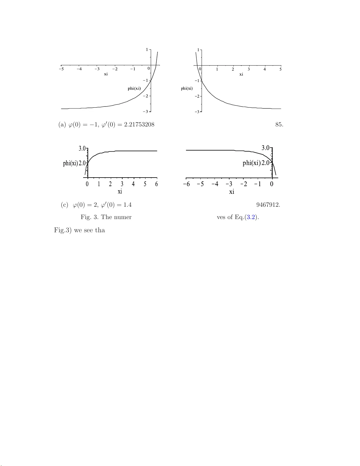
A t yp e of b ounded tra v eling w a v e soluti ons for the F orn b erg-Wh itham equation Jiangb o Zhou ∗ , Lixin Tian Nonline ar Scientific R ese ar ch Center, F aculty of Scie nc e, Jiangsu University, Zhenjiang, J ia ngsu, 2120 13, China Abstract In this pap er, by using bifurcation metho d, we successfully find the F orn b erg- Whitham equation u t − u xxt + u x = uu xxx − uu x + 3 u x u xx , has a t yp e of tra v eling wa ve solutions called kink-lik e wa ve solutions and an tikink- lik e w a ve so lutions. They are defined on some semifinal b ounded domains and p os- sess pr o p erties of kin k wa ves and an ti-kink w av es. T h ei r implicit expressions are obtained. F or some co ncrete d a ta, the graphs o f the implicit functions a re disp l ay ed, and the numerical simulation is made. T h e results sh o w that our th eoretical analysis agrees with the numerical sim ulation. Key wor ds: F orn b erg-Whitham equation, trav eling w a ve solution, bifur c ation metho d 1991 MSC: 34C25-2 8; 34C35; 35B65; 58F05 ∗ Corresp onding author. Email addr ess: zhou jiangbo@yahoo.cn (Jiangb o Z h o u ). Preprint submitted to Elsevier 27 Octob er 2018 1 In tro duction It is w ell kno wn that the exact solutions f or the nonlinear partial differen tial equations can help p eople know deeply the describ ed pro cess. So an imp ortan t issue of the nonlinear partial differen tial equations is to find their new exact solutions. T ra v eling w av e solution is an importa n t t yp e of solution for the nonlinear partial differen tial equations and many nonlinear part ial differen tial equations ha v e been found to ha ve a v ariet y of tr a ve ling w av e solutions. F or instances, the w ell-know n Kortew eg-de V ries equation u t − 6 uu x + u u xxx = 0 (1.1) has solitar y w a ve solutions and its solitary w av es are solitons [ 1 ]. A KdV-lik e equation u t + a (1 + bu n ) u n u x + δ u xxx = 0 (1.2) has some kink wa ve solutions [ 2 ]. Its kink w av e solution u ( ξ )( ξ = x − ct ) w as difined on ( −∞ , + ∞ ), and lim ξ →−∞ u ( ξ ) = A , lim ξ →∞ u ( ξ ) = B , where A and B are t w o constan ts and A 6 = B . The Camassa-Holm equation u t − u xxt + 3 u u x = 2 u x u xx + u u xxx (1.3) has p eak ons, cusp ons , stump ons, comp osite w av e solutions [ 3 ], it also has compactons [ 4 ]. The Degasp eris-Procesi equation u t − u xxt + 4 u u x = 3 u x u xx + u u xxx (1.4) 2 has a multitude of p eculiar w av e solutions: p e akons , cusp ons , comp osite w av es, and stump ons [ 5 ]. The Kuramoto- Siv ashinsky equation u t + u u x + u xx + u xxxx = 0 (1.5) has p erio dic and solitary solutions [ 6 ]. In [ 7 ], Liu, Li and Lin found a new t yp e of trav eling w av e solutions fo r the Camassa-Holm equation, whic h are defined on some semifinal b o un ded domains and p ossess pro p erties of kink w a v es or an ti-kink w av es. They called them kink-lik e w a v es and an tikink-lik e w av es. Later, Guo and Liu [ 8 ] found the CH − γ equation u t + c 0 u x + 3 u u x − α 2 ( u xxt + u u xxx + 3 u x u xx ) + γ u xxx = 0 , (1.6) p osse s kink-like w av es when α 2 > 0. T ang and Zhang [ 9 ] sho w ed the CH − γ equation ( 1.6 ) also has kink-lik e w av e solutions ev en when α 2 < 0. Chen and T ang [ 10 ] sho w ed that the D egasperis-Pro cesi equation ( 1.4 ) has suc h type of tra v eling w av e solutio ns. Recen t ly , Liu a n d Y ao [ 11 ] found the fo llo wing generalized Camass a- H olm equation u t + 2 k u x − u xxt + au u x = 2 u x u xx + u u xxx (1.7) also p osses kink-lik e w av e solutions. W e are motiv ated to seek kink-lik e w a ve and an tikink-lik e w av e solutions for the F ornberg-Whitham equation u t − u xxt + u x = u u xxx − uu x + 3 u x u xx . (1.8) T o our know ledge, suc h t yp e of trav eling w av e solution has nev er b een found for the F orn b erg-Whitham equation. Eq.( 1.8 ) w a s used to study the qualita- 3 tiv e b e haviours of w av e-breaking [ 12 ]. It admits a w a ve of greatest height, as a p eak ed limiting form of the trav eling wa ve solution [ 13 ], u ( x, t ) = A exp( − 1 2    x − 4 3 t    ), where A is a n arbitrary constan t. The remainder of the paper is o rganized a s follo ws. In Section 2, w e state the main results whic h ar e implicit expressions o f the kink -like w a v e and the an tikink-lik e wa ve solutions. In Section 3, we giv e the pro of of t he main re- sults. In Section 4, w e mak e the nume rical sim ulatio n of the kink-like a nd the an tikink-lik e w av es. A short conclusion is g iv en in Section 5. 2 Main results W e state our main result as follows . Theorem 1. F or giv en constan t c , let ξ = x − ct (2.1) ϕ ± 0 = c − 1 ± q ( c − 1) 2 − 2 g (2.2) g 1 ( c ) = ( c − 1 ) 2 2 (2.3) g 2 ( c ) = ( c − 1 ) 2 − 1 2 (2.4) (1) If g < g 2 ( c ), then Eq.( 1.8 ) has tw o kink-lik e w a v e solutions u = ϕ 1 ( ξ ) and u = ϕ 3 ( ξ ) and tw o an tikink-lik e w av e solutions u = ϕ 2 ( ξ ) and u = ϕ 4 ( ξ ). (2 q ϕ 2 1 + l 1 ϕ 1 + l 2 + 2 ϕ 1 + l 1 )( ϕ 1 − ϕ − 0 ) α 1 (2 √ a 1 q ϕ 2 1 + l 1 ϕ 1 + l 2 + b 1 ϕ 1 + l 3 ) α 1 = β 1 e − 1 2 ξ , ξ ∈ ( −∞ , ξ 1 0 ) (2.5) (2 q ϕ 2 2 + l 1 ϕ 2 + l 2 + 2 ϕ 2 + l 1 )( ϕ 2 − ϕ − 0 ) α 1 (2 √ a 1 q ϕ 2 2 + l 1 ϕ 2 + l 2 + b 1 ϕ 2 + l 3 ) α 1 = β 1 e 1 2 ξ , ξ ∈ ( − ξ 1 0 , ∞ ) (2.6) 4 (2 q ϕ 2 3 + m 1 ϕ 3 + m 2 + 2 ϕ 3 + m 1 )( ϕ 3 − ϕ + 0 ) α 2 (2 √ a 2 q ϕ 2 3 + m 1 ϕ 3 + m 2 + b 2 ϕ 2 + m 3 ) α 2 = β 2 e − 1 2 ξ , ξ ∈ ( − ξ 3 0 , ∞ ) (2.7) and (2 q ϕ 2 4 + m 1 ϕ 4 + m 2 + 2 ϕ 4 + m 1 )( ϕ 4 − ϕ + 0 ) α 2 (2 √ a 2 q ϕ 2 4 + m 1 ϕ 4 + m 2 + b 2 ϕ 4 + m 3 ) α 2 = β 2 e 1 2 ξ , ξ ∈ ( −∞ , ξ 3 0 ) (2.8) where l 1 = 2 3 (1 − 3 c − 3 q ( c − 1 ) 2 − 2 g ) (2.9) l 2 = 2 3 [1 − 4 c + 3 c 2 − 3 g + (3 c + 1) q ( c − 1 ) 2 − 2 g ] (2.10) l 3 = 4 3 [2 − 5 c + 3 c 2 − 6 g + (3 c + 2) q ( c − 1 ) 2 − 2 g ] (2.11) m 1 = 2 3 (1 − 3 c + 3 q ( c − 1 ) 2 − 2 g ) (2.12) m 2 = 2 3 [1 − 4 c + 3 c 2 − 3 g − (3 c + 1) q ( c − 1) 2 − 2 g ] (2.13) m 3 = 4 3 [2 − 5 c + 3 c 2 − 6 g − (3 c + 2) q ( c − 1) 2 − 2 g ] (2.14) a 1 = 4(1 − 2 c + c 2 − 2 g + q ( c − 1) 2 − 2 g ) (2.15) a 2 = 4(1 − 2 c + c 2 − 2 g − q ( c − 1 ) 2 − 2 g ) (2.16) b 1 = − 4 3 − 4 q ( c − 1 ) 2 − 2 g (2.17) b 2 = − 4 3 + 4 q ( c − 1 ) 2 − 2 g ( 2 .18) α 1 = − 1 + q ( c − 1 ) 2 − 2 g 2 r ( c − 1 ) 2 − 2 g + q ( c − 1 ) 2 − 2 g (2.19) 5 α 2 = − 1 + q ( c − 1 ) 2 − 2 g 2 r ( c − 1) 2 − 2 g − q ( c − 1 ) 2 − 2 g (2.20) β 0 1 = (2 √ c 2 + l 1 c + l 2 + 2 c + l 1 )( c − ϕ − 0 ) α 1 (2 √ a 1 √ c 2 + l 1 c + l 2 + b 1 c + l 3 ) α 1 (2.21) β 0 2 = (2 √ c 2 + m 1 c + m 2 + 2 c + m 1 )( c − ϕ + 0 ) α 2 (2 √ a 2 √ c 2 + m 1 c + m 2 + b 2 c + m 3 ) α 2 (2.22) β 1 = ln (2 √ a 2 + l 1 a + l 2 + 2 a + l 1 )( a − ϕ − 0 ) α 1 2 √ a 1 √ a 2 + l 1 a + l 2 + b 1 a + l 3 ) α 1 (2.23) β 2 = (2 √ b 2 + m 1 b + m 2 + 2 b + m 1 )( b − ϕ + 0 ) α 2 (2 √ a 2 √ b 2 + m 1 b + m 2 + b 2 b + m 3 ) α 2 (2.24) ξ 1 0 = 2 ln( β 1 /β 0 1 ) (2.25) ξ 3 0 = 2 ln( β 0 2 /β 2 ) (2.26) a and b are t wo constan ts satisfying ϕ 1 (0) = ϕ 2 (0) = a , ϕ 3 (0) = ϕ 4 (0) = b , and ϕ − 0 < a < c < b < ϕ + 0 . (2) If g 2 ( c ) ≤ g ≤ g 1 ( c ), then Eq.( 1.8 ) has a kink-like w av e solution u = ϕ 1 ( ξ ) of implicit form ( 2.5 ) and a a ntikink-lik e w av e solution u = ϕ 2 ( ξ ) of implicit form ( 2.6 ) . W e will give the pro of of this theorem in Section 3. No w w e tak e a set of data and emplo y Maple to displa y the graphs of u = ϕ i ( ξ )( i = 1 , 2 , 3 , 4). Example 1. T aking c = 1 and g = − 4 < g 2 ( c ) (correspo nd ing t o (1) of Theorem 1), it follows that ϕ − 0 = − 2 . 82 843, ϕ + 0 = 2 . 8 2843, l 1 = − 6 . 99019 and l 2 = 15 . 54 2 5, l 3 = 50 . 85 6 2, a 1 = 43 . 3137, b 1 = − 12 . 647 , α 1 = − 0 . 58171 2. F urther, choosing a = − 1 ∈ ( ϕ − 0 , c ), w e obta in ξ 1 0 = 0.387475. W e presen t the graphs of the solutions ϕ 1 ( ξ ) and ϕ 2 ( ξ ) in Fig.1 (a) and (b) resp ectiv ely . Mean while, w e get m 1 = 4 . 3 2352 and m 2 = 0.457528, m 3 = 13.1438, a 2 = 6 x K 6 K 5 K 4 K 3 K 2 K 1 0 f 1 K 3 K 2 K 1 1 (a) x 0 1 2 3 4 5 6 f 2 K 3 K 2 K 1 1 (b) x 0 1 2 3 4 5 6 f 3 1.5 2.0 2.5 3.0 (c) x K 6 K 5 K 4 K 3 K 2 K 1 0 f 4 1.5 2.0 2.5 3.0 (d) Fig. 1. Th e graphs of ϕ i ( ξ )( i = 1 , 2 , 3 , 4) wh e n c = 1, g = − 4, a = − 1, b = 2. 20.6863, b 2 = 9.98038, α 2 = 0.40201. F urther, choosing b = 2 ∈ ( c, ϕ + 0 ), w e get ξ 3 0 = 0.2747 8 7 . The gra phs of the solutions ϕ 3 ( ξ ) a nd ϕ 4 ( ξ ) a r e pr esen ted in Fig.1(c) and (d) resp en t ively . The graphs in Fig.1 show that ϕ 1 ( ξ ) and ϕ 3 ( ξ ) are kink-lik e w a ve s and ϕ 2 ( ξ ) and ϕ 4 ( ξ ) are antikink -like w av es. 3 Pro of of main results Let u = ϕ ( ξ ) with ξ = x − ct b e the solution for Eq.( 1.8 ), then it follo ws that − cϕ ′ + cϕ ′′′ + ϕ ′ = ϕϕ ′′′ − ϕϕ ′ + 3 ϕ ′ ϕ ′′ (3.1) In tegrating ( 3.1 ) once w e ha v e ϕ ′′ ( ϕ − c ) = g − cϕ + ϕ + 1 2 ϕ 2 − ( ϕ ′ ) 2 (3.2) 7 where g is the in tegral constan t. Let y = ϕ ′ , t hen w e get the follo wing planar system                dϕ dξ = y dy dξ = g − cϕ + ϕ + 1 2 ϕ 2 − y 2 ϕ − c (3.3) with a first in tegra l H ( ϕ, y ) = ( ϕ − c ) 2 [ y 2 − ( ϕ − c ) 2 4 − 2 3 ( ϕ − c ) − g − c + c 2 2 ] = h (3.4) where h is a constan t. Note that ( 3.3 ) has a singular line ϕ = c . T o a v oid the line temp orarily w e mak e transformation dξ = ( ϕ − c ) dζ . Under this transformation, Eq.( 3.3 ) b ecome s                dϕ dζ = ( ϕ − c ) y dy dζ = g − cϕ + ϕ + 1 2 ϕ 2 − y 2 (3.5) The Eq.( 3.3 ) and Eq.( 3.5 ) hav e the same first in tegral as ( 3.4 ). Consequen tly , system ( 3.5 ) has the same top ological phase p ortraits as system ( 3.3 ) except for the straight line ϕ = c . Ob viously , ϕ = c is an inv ar ian t straigh t-line solution f or system ( 3.5 ). No w w e consider the singular p oin ts of sys tem ( 3.5 ) a nd their pro perties . Note tha t for a fixed h , ( 3.4 ) determines a set of in v ar ia n t curv es o f ( 3.5 ). As h is v aried ( 3.4 ) determines differen t families of orbits of ( 3.5 ) hav ing differen t dynamical b eha viors. Let M ( ϕ e , y e ) b e the co efficien t matrix of the linearized 8 system of ( 3.5 ) at the equilibrium p oin t ( ϕ e , y e ), then M ( ϕ e , y e ) =         y e ϕ e − c ϕ e − ( c − 1) − 2 y e         and a t this equilibrium p o in t, w e hav e J ( ϕ e , y e ) = det M ( ϕ e , y e ) = − 2 y 2 e − ( ϕ e − c )[ ϕ e − ( c − 1 )] , p ( ϕ e , y e ) = tr ace ( M ( ϕ e , y e )) = − y e . By the theory of planar dynamical system (see [ 14 ]), for an equilibrium p oin t of a planar dynamical system, if J < 0, then this equilibrium p oin t is a saddle p oin t ; it is a cen ter p oin t if J > 0 a nd p = 0; if J = 0 a n d the P oinc´ are index of the equilibrium p o in t is 0, then it is a cusp. Since system ( 3.3 ) has the same top ological phase p ortraits as system ( 3.5 ) except for the straigh t line ϕ = c . By in v estigating the top ological dynamics of system ( 3.5 ), we can obta in the fo llowing prop erties for syste m ( 3 .3 ). (1) If g < g 2 ( c ), then system ( 3.4 ) has t w o equilibrium p oin ts ( ϕ − 0 , 0) a nd ( ϕ + 0 , 0). They are saddle p oin ts and there is inequalit y ϕ − 0 < c − 1 < c < ϕ + 0 . In this case, there are fo u r orbits connecting with ( ϕ − 0 , 0), w e use l 1 ϕ − 0 and l 2 ϕ − 0 to denote the t w o orbits lying on the righ t side of ( ϕ − 0 , 0) ( see Fig.2(a )). Mean while, there a re four o rbits connecting with ( ϕ + 0 , 0), w e employ l 1 ϕ + 0 and l 2 ϕ + 0 to denote the t w o orbits lying on the left side of ( ϕ + 0 , 0) (see Fig.2(a )). (2) If g 2 ( c ) ≤ g ≤ g 1 ( c ), then system ( 3.4 ) ha s t w o equilib rium p oin t s ( ϕ − 0 , 0), ( ϕ + 0 , 0). ( ϕ − 0 , 0) is a saddle p oin t and ( ϕ + 0 , 0) is a cen ter p oin t or a degenerate cen ter p oin t. ϕ − 0 and ϕ + 0 satisfy that ϕ − 0 < c − 1 < ϕ + 0 < c . l 1 ϕ − 0 and l 2 ϕ − 0 are 9 used t o denote the t w o orbits lying on the righ t side of ( ϕ − 0 , 0) (see Fig.2(b)) (3) If g 1 ( c ) < g , then system ( 3.4 ) has no equilibrium p oin t. c ! 1 0 " ! l 1 0 # ! l ! 2 0 # ! l ) ( 1 $ ! ) ( 3 ! $ ) ( 4 $ ! # 0 ! ) ( 2 $ ! " 0 ! 2 0 " ! l (a) g < g 2 ( c ) c ! 1 0 " ! l ) ( 1 # ! ) ( 2 # ! " 0 ! ! 2 0 " ! l (b) g 2 ( c ) ≤ g ≤ g 1 ( c ) Fig. 2. Th e sk etc hes of orbits connecting w ith saddle p oin ts. On the ϕ − y plane, the orbits l 1 ϕ − 0 , l 2 ϕ − 0 , l 1 ϕ + 0 and l 2 ϕ + 0 ha v e the follo wing expressions resp ectiv ely . l 1 ϕ − 0 : y = 1 2 ( ϕ − ϕ − 0 ) √ ϕ 2 + l 1 ϕ + l 2 c − ϕ (3.6) l 2 ϕ − 0 : y = 1 2 ( ϕ − 0 − ϕ ) √ ϕ 2 + l 1 ϕ + l 2 c − ϕ (3.7) l 1 ϕ + 0 : y = 1 2 ( ϕ + 0 − ϕ ) √ ϕ 2 + m 1 ϕ + m 2 ϕ − c (3.8) l 2 ϕ + 0 : y = 1 2 ( ϕ − ϕ + 0 ) √ ϕ 2 + m 1 ϕ + m 2 ϕ − c (3.9) where ϕ − 0 and ϕ + 0 are in ( 2.2 ), l 1 and l 2 are in ( 2 .9 ) and ( 2.10 ), m 1 and m 2 are in ( 2 .12 ) and ( 2.13 ). Assume that ϕ = ϕ 1 ( ξ ), ϕ = ϕ 2 ( ξ ), ϕ = ϕ 3 ( ξ ) and ϕ = ϕ 4 ( ξ ) on l 1 ϕ − 0 , l 2 ϕ − 0 , l 1 ϕ + 0 and l 2 ϕ + 0 resp e ctiv ely and ϕ 1 (0) = ϕ 2 (0) = a , ϕ 3 (0) = ϕ 4 (0) = b , where a and b are tw o constan ts, and a ∈ ( ϕ − 0 , c ), b ∈ ( c, ϕ + 0 ). Substituting ( 3.6 )-( 3.9 ) in to t he first equation of ( 3.3 ) and in tegrating alo n g the corresp onding orbits 10 resp e ctiv ely , w e ha v e ϕ 1 Z a c − s ( s − ϕ − 0 ) √ s 2 + l 1 s + l 2 ds = 1 2 ξ Z 0 ds (along l 1 ϕ − 0 ) (3.10) a Z ϕ 2 c − s ( ϕ − 0 − s ) √ s 2 + l 1 s + l 2 ds = 1 2 0 Z ξ ds (along l 2 ϕ − 0 ) (3.11) b Z ϕ 3 s − c ( ϕ + 0 − s ) √ s 2 + m 1 s + m 2 ds = 1 2 0 Z ξ ds (along l 1 ϕ + 0 ) (3.12) ϕ 4 Z b s − c ( s − ϕ + 0 ) √ s 2 + m 1 s + m 2 ds = 1 2 ξ Z 0 ds (along l 2 ϕ + 0 ) (3.13) Computing the ab o ve four in tegrals w e obtain the implicit expressions of ϕ i ( ξ ) as ( 2.5 )-( 2.8 ). Mean while, suppo s e that ϕ 1 ( ξ ) → c as ξ → ξ 1 0 , ϕ 2 ( ξ ) → c a s ξ → − ξ 2 0 , ϕ 3 ( ξ ) → c as ξ → − ξ 3 0 , ϕ 4 ( ξ ) → c as ξ → ξ 4 0 , t hen it follo w fr o m ( 3.10 ) - ( 3.13 ) that ξ 1 0 = ξ 2 0 = c Z a c − s ( s − ϕ − 0 ) √ s 2 + l 1 s + l 2 ds (along l 1 ϕ − 0 ) (3.14) ξ 3 0 = ξ 4 0 = c Z b s − c ( s − ϕ + 0 ) √ s 2 + m 1 s + m 2 ds (along l 2 ϕ + 0 ) (3.15) Computing the ab o v e t w o integrals, we get the expressions of ξ 1 0 and ξ 3 0 as in ( 2.25 ) a n d ( 2.26 ). The pro of is finished. 4 Numerical sim ulations In this section, we will sim ulat e the planar gra phs of the kink-lik e and the an tikink-lik e w av es. 11 F rom Section 3, w e see that in the parameter expressions ϕ = ϕ ( ξ ) and y = y ( ξ ) of the orbits of System ( 3.3 ), the graph of ϕ ( ξ ) and the in tegral curv e of Eq.( 3.2 ) are the same. In other words, the integral curv es of Eq.( 3.2 ) are the planar gra phs of the tra ve ling w av es of Eq.( 1.8 ). Therefore, w e can see the planar graphs of the kink-lik e and the antikink-lik e wa ves through the sim ulation of the in tegral curv es of Eq.( 3.2 ). Example 2. T ak e the same data as Example 1, tha t is c = 1, g = − 4, a = − 1, b = 2. Let ϕ = a = − 1 in ( 3.6 ) and ( 3 .7 ), then we can get y ≈ 2 . 2175320 85 or y ≈ − 2 . 217532 085. And let ϕ = b = 2 in ( 3.8 ) and ( 3 .9 ), then w e obta in y ≈ 1 . 4994 67912 or y ≈ − 1 . 499 4 67912. Th us w e tak e the initial conditions o f Eq.( 3.2 ) as follow s: (i) Corresp onding to l 1 ϕ − 0 w e tak e ϕ ( 0) = − 1 and ϕ ′ (0) = 2 . 21 7532085. (ii) Corresp onding to l 2 ϕ − 0 w e tak e ϕ (0) = − 1 and ϕ ′ (0) = − 2 . 21753 2085. (iii) Corresponding to l 1 ϕ + 0 w e tak e ϕ (0) = 2 and ϕ ′ (0) = 1 . 4 99467912. (iv) Corresp onding to l 2 ϕ + 0 w e ta k e ϕ (0) = 2 and ϕ ′ (0) = − 1 . 49946791 2 . Under each set of initial conditions w e use Maple to sim ulate the integrals curv e of Eq.( 3.2 ) as Fig.3. Comparing Fig.1 with Fig.3 , w e can see that the graphs of ϕ i ( ξ )( i = 1 , 2 , 3 , 4) are t he same as the sim ulatio n of in tegrals curv e of Eq.( 3.2 ). This implies that our theoretic results agree with the n umerical sim ulations. 5 Conclusion In this pap er, w e find new b ounded w a ve s for the F orn b erg-Whitham equa- tion ( 1.8 ). Their implicit expressions are obtained in ( 2.5 )-( 2.8 ). F r o m the graphs (see Fig.1) of the implicit functions and the n umerical sim ulations (see 12 xi K 5 K 4 K 3 K 2 K 1 0 phi(xi) K 3 K 2 K 1 1 (a) ϕ (0) = − 1, ϕ ′ (0) = 2 . 217 532085. xi 0 1 2 3 4 5 phi(xi) K 3 K 2 K 1 1 (b) ϕ (0) = − 1 , ϕ ′ (0) = − 2 . 2175 32085. xi 0 1 2 3 4 5 6 phi(xi) 2.0 3.0 (c) ϕ (0) = 2, ϕ ′ (0) = 1 . 499 467912. xi K 6 K 5 K 4 K 3 K 2 K 1 0 phi(xi) 2.0 3.0 (d) ϕ (0) = 2, ϕ ′ (0) = − 1 . 4994 67912. Fig. 3. The n um er ical simulat ions of integ ral cu rv es of Eq.( 3.2 ). Fig.3) w e see that these new b ounded solutions are defined on some semifinal b ounded domains and p osses s prop erties of kink wa ves and an ti-kink w a v es. References [1] J. Lenells, T ra ve ling w a v e solutions of the Camassa-Holm and Kortew eg-de V r ie s equations, J . Nonlinear Math. Phys. 11 (2004) 508-520. [2] B. Dey , Domain wall solutions of Kd V lik e equations with higher order nonlinearit y . J. Phys. A: Math. Gen. 19 (1986 ) L9-L12. [3] J. Lenells, T r a v eling wa ve solutions of the Camassa-Holm equation, J. Differen tial Equations 217 (2005) 393-43 0. [4] Z. Liu, C. C hen, Compactons in a general compr e ssib l e hyperelastic ro d, Chaos, Solitons an d F r a ctals 22 (2004) 627-64 0. 13 [5] J. Lenells, T ra ve ling wa v e solutions of the Degasp eris-Procesi equation, J . Math. Anal. Ap pl. 306 (2005) 72-82. [6] J. Nic kel , T rav elling wa ve solutions to the Kuramoto-Siv ashinsky equation, Chaos, Solitons and F ractals 33 (2007) 1376- 1382. [7] Z. Liu, Q. Li, Q . Lin, New b ounded tra veling wa v es of Camassa-Holm equation, In t. J. Bifurcat. C hao s 14 (2004 ) 3541- 3556. [8] B. Guo, Z . Liu, Two new t yp es of b ound ed w a ves of CH- γ equation, Science in China Ser. A: Mathematics 48 (2005 ) 1618- 1630. [9] M. T ang, W. Zhang, F our t yp es of b ounded wa v e solutions of CH- γ equation, Science in Chin a Ser. A: Mathematics 50 (2007) 132-152. [10] C. Chen, M. T ang, A n ew t yp e of b ound e d w av es for Degasp e ris-Pr ocesi equation, Ch a os, Solitons and F ractals 27 (2006 ) 698-7 04. [11] Z. Liu, L. Y ao, Compacton-lik e w a v e and kink-lik e wa v e of GCH equation, Nonlinear An a lysis: Real W orld Applications 8 (2007) 136-1 55. [12] G. B. Whitham, V ariational metho ds and applications to w ater wa ve, Pro c. R. So c. Lond. A 299 (1967) 6-25. [13] B. F ornberg, G. B. Whitham, A n umerical and theoretical stud y of certain nonlinear wa ve p henomena, Phil. T rans. R. So c. Lond. A 289 (1978) 373-404. [14] D. Lu o et al., Bifur c ation Theory and Met ho ds of Dynamical S yste ms, W orld Scien tific Publish i ng Co. Pvt. Ltd., London, 1997. 14