Distributed MIMO radar using compressive sampling

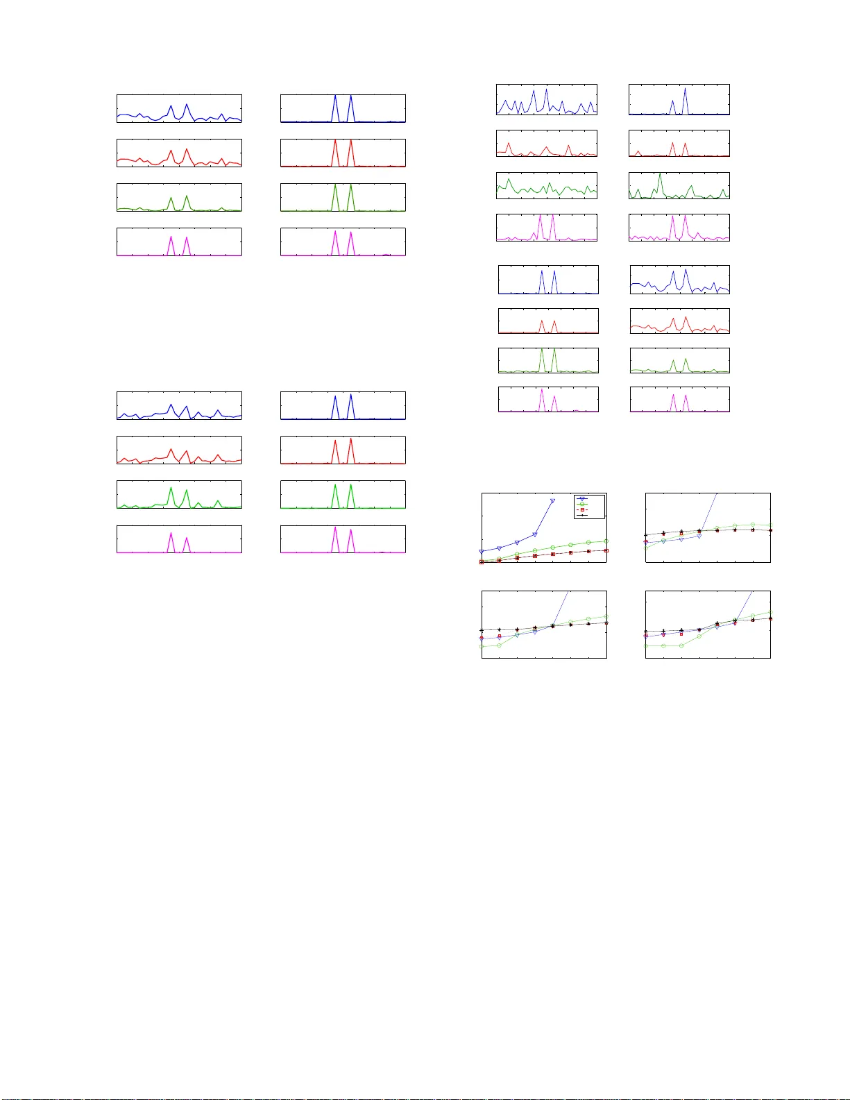
Distrib uted MIMO Radar Using Compressi v e Sampling Athina P . Petropulu, Y ao Y u and H. V ince nt Poor + Electrical & Computer E ngineer ing Departmen t, Drexel Univ ersity + School of Engineer ing and App lied Scien ce, Pr inceton Un iv ersity Abstract — A distributed MIMO radar is consider ed, in which the transmit and receiv e antennas belong to nodes of a small scale wireless network. The transmit wav ef orms could be u ncorrelated, or corr elated in order to achiev e a desirable beampattern. The concept of compres sive sampling is employ ed at th e recei ve nodes in order to perf orm direction of arriva l ( DO A) estimation. According to the theory of compressiv e samplin g, a signal that is sp arse in some domain can be recov ered b ased on far fewer samples than required by the Nyqu ist sampling theorem. Th e DO As of targ ets f orm a sparse vector in the angle space, and theref ore, compre ssiv e sampling can be applied for DOA esti- mation. Th e p roposed approach achieves the superior res olution of MIMO radar with far fewer samples t han other approaches. This is particul arly useful in a distributed scenario, in wh ich the results at each receiv e n ode need to be transmitted to a fusion center . K eywords: Compressi ve samplin g, M IMO Radar , DOA Esti- mation I . I N T RO D U C T I O N A multiple-inp ut multiple- outpu t (MIMO) radar system, as originally prop osed in [1]-[5] transmits mu ltiple ind ependen t wa vefo rms v ia its antennas. Consider a MIM O r adar equippe d with M t transmit and M r receive antennas that ar e close to each other r elativ e to th e target. The phase differences induced by tran smit and receive anten nas can be exploited to form a long virtua l array with M t M r elements. This enables the M IMO radar system to achieve super ior sp atial resolution as compa red to a traditio nal radar system. MIMO radar transmitting correlated signal waveforms in ord er to achieve a desired beamp attern has also been p ropo sed [ 10]- [12]. This is useful in cases wh ere th e rad ar system wishes to avoid c ertain d irections, be cause they either correspo nd to eav esdropp ers, or ar e kn own to b e o f no interest. Compressive sensing (CS) h as received considerable atten- tion recently , and has been app lied succe ssfully in d iv erse fields, e.g ., image p rocessing [6] and wireless commun ications [7]. Th e theory of CS states that a K -sparse signal x of length N can be recovered exactly with high probab ility from O ( K log N ) measuremen ts via linear pr ogramm ing. Let Ψ denote the basis matrix that sp ans this sparse space , an d let Φ den ote a measurement matr ix. The c onv ex optimization problem arising from CS is fo rmulated as follows: min k s k 1 , subject to y = Φ x = ΦΨ s (1) where s is a sp arse vector with K prin cipal elem ents and the remaining ele ments can be igno red; Φ is an M × N matrix incohere nt with Ψ and M ≪ N . In th is paper, we p ropose a distributed MIM O r adar system, where tr ansmit and receive antennas b elong to no des of a wireless network that are unifo rmly distributed on a disk or a certain ra dius. loca ted wireless network node s. The readin gs of the receive nodes are transmitted to a cen tral node f or DO A estima tion. Energy efficiency is an importan t issue in such a wireless n etwork as the no des op erate o n b attery . W e employ the idea of compressive sampling in order to save in energy consume d during d ata tra nsmission to the central n ode. Recently , the work of [8] considere d DO A estimation o f signal sources using CS. I n [ 8], the basis matrix Ψ is f ormed by the discretization of the angle space. The source signals wer e assumed to be u nknown, an d an appr oximate version of the basis matrix was obtained based on the sig nal received by a referenc e v ector . The signal at the ref erence sensor would hav e to be sampled at a very high rate in order to construct a good basis matrix . Her e, we extend th e idea of [8] to the problem of DO A estimation for MIM O radar . Since the n umber of targets is typically smaller than the num ber of sn apshots that can be obtained, DOA estimation can b e for mulated as the rec overy of a sparse vector using CS. Unlike the scenario consider ed in [8], in MI MO rad ar the tr ansmitted wav eforms are known at eac h receive an tennas. This enables each receiv e an tenna to construct the basis m atrix locally , without knowledge o f the received signal at a reference sen sor or any other antenna. W e consider the more general case of correlated signal wa vefo rms. W e provide analytical expressions for th e a verage signal-to - jammer ratio (SJR) fo r the pr oposed appro ach. Simulation results show that the pro posed approac h can accomplish the super-resolution of MIMO radar systems while using far fewer samples than existing methods, such as Capon, amplitude and phase estimation (APES) and generalized likelihood ratio te st (GLR T) [2]. I n particular, the propo sed ap proach can enab le each n ode to o btain a good DO A estimate in depend ently . Further, it results in mu ch less inform ation to be tra nsmitted to a fusion c enter, thus enab ling savings in ter ms of tran smission energy . I I . S I G N A L M O D E L F O R M I M O R A DA R W e c onsider a MIMO rad ar system with M t transmit node s and M r receive no des that are uniformly distributed o n a disk of radiu s r . For simp licity , we assume th at targets and nodes lie on the same plan e. Fur ther, we assume that each n ode in the network kn ows which are th e nodes that serve are tr ansmit and receive anten nas a nd what th eir coord inates ar e relative to a fixed p oint in th e network. Th is in formatio n can be provided by a hig her network la yer . Let us d enote the locatio ns in rectangu lar coo rdinates of the i -th tr ansmit and recei ve antenna by ( x t i , y t i ) an d ( x r i , y r i ) , respectively (see Fig.1). The location of the k - th target is denoted b y the po- lar coordina tes ( d k , θ k ) , where d k is the distance between this target and the or igin, and θ k is the azimuthal angle, which is the unknown parameter to be e stimated in this paper . Under the far-field assump tion d k ≫ p ( x t i ) 2 + ( y t i ) 2 and d k ≫ p ( x r i ) 2 + ( y r i ) 2 , the distance between the i th transmit/receive antenna and the k -th target d t ik / d r ik can be approx imated as d t/r ik ≈ d k − η t/r i ( θ k ) , where η t/r i ( θ k ) = x t/r i cos( θ k ) + y t/r i sin( θ k ) . Let x i ( n ) denote th e discrete-time wa veform tran smitted b y the i -th transmit antenna. Assuming the transmitted w av eforms are n arrowband and the p ropag ation is non- dispersive, the received baseband signal at the k - th target equals [4] y k ( n ) = β k M t X i =1 x i ( n ) e − j 2 π λ d t ik = β k e − j 2 π λ d k x T ( n ) v ( θ k ) k = 1 , . . . , K (2) where λ is the tra nsmitted signal wavelength, v ( θ k ) = [ e j 2 π λ η t 1 ( θ k ) , ..., e j 2 π λ η t M t ( θ k ) ] T (3) x ( n ) = [ x 1 ( n ) , ..., x M t ( n )] T . (4) Due to reflection by th e target, the l -th antenna element receives z l ( n ) = K X k =1 e − j 2 π λ d r lk y k ( n ) + ǫ l ( n ) , l = 1 , . . . , M r (5) where ǫ l ( n ) rep resents ind epende nt and identically distributed (i.i.d.) Ga ussian noise with variance σ 2 . On letting L d enote the n umber of snapshots, we have z l =    z l (0) . . . z l ( L − 1)    = K X k =1 e − j 2 π λ d r lk y k + e l = K X k =1 e − j 2 π λ (2 d k − η r l ( θ k )) β k Xv ( θ k ) + e l (6) where y k = [ y k (0) , . . . , y k ( L − 1)] T , e l = [ ǫ l (0) , . . . , ǫ l ( L − 1)] T and X = [ x (0) , . . . , x ( L − 1)] T . By discretizing the angle space as a = [ α 1 , . . . , α N ] , we can r ewrite (7) as z l = N X n =1 e j 2 π λ η r l ( α n ) s n Xv ( α n ) + e l (7) k The k -th target x y i i k t t i i ( , ) x y r r i i ( , ) x y Fig. 1. MIMO Radar System where s n =  e − j 4 π λ d k β k if ther e is ta rget at α n 0 other wise . I I I . C O M P R E S S I V E S E N S I N G F O R M I M O R A DA R Assuming that there exists a small numb er of targets, the DO As are spa rse in the an gle space , i.e., s = [ s 1 , . . . , s N ] is a sparse vector . A no n-zero element with index j in s in dicates that the re is a target at the angle α j . By CS th eory , we can constru ct a basis m atrix Ψ l for the l -th anten na as Ψ l = [ e j 2 π λ η r l ( α 1 ) Xv ( α 1 ) , . . . , e j 2 π λ η r l ( α N ) Xv ( α N )] . (8) Ignor ing the noise, we have z l = Ψ l s . T hen we m easure linear pro jections of the r eceived signal at the l -th an tenna as r l = Φ l z l = Φ l Ψ l s , (9) where Φ l is an M × L rando m Gaussian matrix which has small cor relation with Ψ l . Comb ining the o utput of N r receive antennas, we h ave r =    r 1 . . . r N r    =    Φ 1 Ψ 1 . . . Φ N r Ψ N r    | {z } Θ s , 1 ≤ N r ≤ M r . (10) Therefo re, we can recover s by applying the Dantzig selector to the c onv ex pro blem in (10) as in [9]: ˆ s = min k s k 1 s.t. k Θ H ( r − Θ s ) k ∞ < µ. (11) According to [ 9], we c an r ecover the sp arse vector s with very high p robability if we select µ = (1 + t − 1 ) p 2 lo g N σ 2 , whe re t is a p ositiv e scalar and σ 2 is the noise p ower . I V . P E R F O R M A N C E A N A L Y S I S I N T H E P R E S E N C E O F A JA M M E R S I G N A L In the p resence of a jam mer at location ( d, θ ) the signal received at the l -th receive antenna ca n b e represented as r l = Φ l K X k =1 e − j 2 π λ (2 d k − η r l ( θ k )) β k Xv ( θ k ) +Φ l e − j 2 π λ ( d − η r l ( θ )) β b + Φ l e l . (12) where β , b den ote respectively the r eflection amplitu de and wa vefo rm of this jammer . Since b is uncor related with the transmitted wav eforms X , the effect of the jammer signal is similar to tha t of addictive noise. Let A l = Φ H l Φ l and D l = X H A l X , wher e D ( i, j ) denotes the ( i, j ) th elem ent of D . W e assume that the T X/RX nod es are uniformly distributed on a d isk with the rad ius r . Thu s, the av erage p ower of the desirable signal P s ( l ) can be r epresented by P s ( l ) = E { K X k,k ′ =1 e j 2 π λ [2( d k − d k ′ ) − ( η r l ( θ k ) − η r l ( θ k ′ )) | {z } ρ l ( k,k ′ ) β ∗ k β k ′ × v H ( θ k ) X H A l Xv ( θ k ′ ) | {z } Q kk ′ } = E { K X k =1 | β k | 2 Q kk } + E { X k 6 = k ′ ρ l ( k , k ′ ) β ∗ k β k ′ Q kk ′ } (13) where Q kk ′ = P i,j D l ( i, j ) e j 2 πr λ ( η t j ( θ k ′ ) − η t i ( θ k )) . Follo wing [3] , we k now that f h ( h ) = 2 π √ 1 − h 2 , − 1 < h < 1 if h = ˜ r r sin (Ψ) , wher e f ˜ r ( ˜ r ) = 2 ˜ r r 2 , 0 < ˜ r < r and f ψ ( ψ ) = 1 2 π , − π < ψ < π . Then E { e j αh } = 2 J 1 ( α ) α , where J 1 ( · ) is the first-or der Bessel functio n of the first kind. Using this proper ty and lettin g a ij = η t/r j ( θ k ′ ) − η t/r i ( θ k ) , we have E { e j 2 πr λ a ij } =  η (4 sin( θ k ′ − θ k 2 )) i = j η 2 (2) i 6 = j (14) where η ( x ) = 2 J 1 ( x πr λ ) x πr λ . Therefo re, th e av erage power of th e desirable signal P s ( l ) taken over the positions of TX/RX no des can be fo und to be: P s ( l ) = K X k =1 | β k | 2 [ X i D l ( i, i ) + X i 6 = j D l ( i, j ) η 2 (2)] + X k 6 = k ′ β ∗ k β k ′ e j 4 π λ ( d k − d k ′ ) η (4 sin( θ k ′ − θ k 2 )) | {z } η kk ′ × [ η kk ′ X i D l ( i, i ) + X i 6 = j D l ( i, j ) η 2 (2)] . (15) Similarly , th e power of th e jamm er sign al is g iv en by P j ( l ) = ( e − j 2 π λ ( d − η r l ( θ )) β )( e − j 2 π λ ( d − η r l ( θ )) β ) ∗ × b H A l b = | β | 2 b H A l b . (16) The SJR giv e n the node locations is the ratio of the po we r of the signal over the power of the ja mmer . Since the deno minator does not depen d on n ode loc ations, the average SJR equ als the ratio o f ( 15) and (16). Since th e jammer sig nal is uncor related with th e transmitted signal, the SJR can be improved by correlatin g the jammer signal with the transmitted signal. Co mbining this with CS, the m easurement m atrix in (9 ) is modified a s ˜ Φ l = Φ l X H . (17) Moreover , since Φ l is a Gaussian rand om m atrix, ˜ Φ l is still Gaussian; ther efore it satisfies the restricted iso metry p roper ty (RIP) an d is in coheren t with Ψ l , thus gu aranteeing a stable solution to (1 1). Based on (17), th e average power of the desir- able sign al P s ( l ) is e qual to (15) except D l = X H XA l X H X . The a verag e power of the jammer signal using ˜ Φ l is re wr itten as P j ( l ) = | β | 2 b H XA l X H b . Approx imating X H X ∼ I M t and using b H b = 1 , the SJRs based o n Φ l and ˜ Φ l can b e appro ximated as M t P K k =1 | β k | 2 | β | 2 and L P K k =1 | β k | 2 | β | 2 , respectively . Theref ore, the SJR using ( 17) can be generally imp roved by a factor o f L / M t since L ≫ M t . the DO A estimates can be imp roved by the increase in L . Howe ver, the time d uration o f the rad ar pu lse might need to be lo nger as well. As simulation resu lts show (see Section V), the proposed method can yield good pe rforma nce even using a single re- ceiv e antenna. W ith a good initial estimate of DO A, the recei ve nodes can adaptively refine their estima tes by co nstructing a higher resolution b asis matrix Ψ l around that DO A. Restricting the candidate angle space, may redu ce the samples in the angle space that are r equired fo r constru cting the basis matrix, thus reducing the complexity of th e ℓ 1 minimization step . On the other hand, the resolutio n of target detection can b e im proved by takin g the de nser samples o f the ang le space aro und the intimal DOA estimate. Furthermo re, the transmit node c an design the corr elated wa veform s fo r transmit beamf orming as well based o n th e g ood initial estimate. V . S I M U L AT I O N R E S U LT S In this section, we con sider a MI MO radar system with the transmit/receive an tennas uniformly distributed on a disk of radius 10 m. The n umber of transmit nodes is fixed at M t = 50 . The carrier freq uency is 8.62 GHz. A m aximum of L = 51 2 snapshots are considered at the receiv e node. The received signal is corrupted by zero mean Gaussian noise. The SNR is set to 20 d B . There are two targets located at θ k = − 1 o , 1 o , with reflection coefficients β k = 1 , k = 1 , 2 . A jammer is lo cated at 15 o and transmits an unknown Gau ssian random wa vefor m and with am plitude 20 , i.e., 26 dB above the target r eflection coefficients β k . W e sample the angle space b y in crements of 0 . 5 o from − 8 o to 8 o , i.e., a = [ − 8 o , − 7 . 5 o , . . . , 7 . 5 o , 8 o ] . First, we compare the pe rforma nce o f DO A estimation using the pro posed method an d three ap proach es [2], i.e., th e Capon, APES and GLR T techniques. Fig. 2 and Fig. 3 show th e modulii of the estimated reflection coef ficients β k , as functions of the azimuthal angle fo r N r = 1 and 1 0 receive antennas, respectively . In Fig. 2, we use the uncor related QPSK wave- forms; while in Fig. 3, we use correlated wa veform s designed accordin g to the desired b eampattern P d ( α n ) as P d ( α n ) =  1 − 3 o ≤ α n ≤ 3 o 0 − 8 o ≤ α n < − 3 o and 3 o < α n ≤ 8 o . (18) Based on that beampattern, the method of [10] was follo wed to design R . Then th e transm itted wa vefo rms can b e constructed as x ( n ) = R 1 2 w , wher e w is a i.i.d rand om vector with zero mean and E { ww H } = I /L . In b oth (a) and (b), the top three c urves cor respond to the azimuthal estimates obtained via Capon, APES and GLR T , using 51 2 snapsho ts. The bottom curve is the result of the propo sed approach, obtained using 35 snapsho ts only . One can see that in the case of using only o ne receive n ode, the presence of the two targets is clearly e vident via the propo sed metho d b ased on 35 sna pshots only using bo th inde- penden t a nd correlated wa vefor ms. The other methods produce spurious pe aks away from the target locations. Whe n the measuremen ts o f multiple receive n odes ar e used at a fusion center, the propo sed ap proach can yield similar perf ormanc e to the o ther th ree me thods. Howe ver , the comparison me thods would hav e to tran smit to the fusion center 512 recei ved samples eac h, wh ile in the proposed appr oach, each node would ne ed to tran smit 35 sam ples each . The thr eshold µ in (11) affects DOA estimation fo r the propo sed method. Th e in crease in µ while keepin g M t and N t constant can red uce the rip ples of DO A estimates at the non- target azimu th an gles at the expense o f the accu racy of the target-reflection- coefficient estimates. Th e increase in µ can also reduce the com plexity of (11) bec ause the constrain t is looser than that o f smaller µ . If µ is to o large, howe ver, the ℓ 1 - norm min imization does not work . In Fig.2 and 3 , relatively large threshold s, i.e., µ = 1 2 , 1 0 , were used for the single receive node case. As a result, the CS method yielded less accurate estimates of the r eflection coefficients magnitud e than the Capon an d APE S, but with very f ew ripples. Finally , we discuss the effect o f L , N t and M t on the perfor mance of the Capon, APES, GLR T and CS. Fig. 4 compare s the perfo rmance o f these four approache s using indepen dent wa veform s for different combination s of N r and L , whose product is fixed at 5 12 . In order to qua ntify the perfor mance o f DO A estimation, we define the ratio of the square am plitude of the DO A estimate at the target azim uth angle to the sum of the square amplitud e of DOA estimates at other angles as th e peak- to-ripple ratio (PRR). Fig. 5 com pares PRR as a fu nction of L f or these fou r approach es using uncorr elated sign al wa vefo rms. W e consider the scenarios in which N r = 1 , 5 , 10 , 30 . For fixed N t and M t , the incr ease in L can im prove the per forman ce of these four method s. In the pr esence o f a moder ate jammer, APES and CS can yield relativ ely accurate DO A estimates even with a small L . For Capon and GLR T , N r must be greater than L in or der to obtain a nonsingular sam ple cov arian ce matrix of the r eceived sign al ˜ R . This is because Capon and GLR T need to calculate the in verse o f ˜ R . On the o ther hand, an incr ease in b oth M t and N r can also imp rove the p erform ance of th e Capon, APES, GLR T and CS wh ile L is fixed. If either M t or N r is too small, even a significant increase in the oth er parameter cann ot improve perfor mance of the first thr ee approac hes. Howe ver, CS can y ield the desired DOA estimates ev e n with a sing le receive antenn a with a sufficient L and N t . In the senecio s considered in our simulations wh ere L = 2 9 , f or instance, M t and N r are req uired to be greater than 8 to yield the desired DO A estima tes using the Capon, APES and GL R T . With a single r eceive n ode, CS require s at least 20 tran smit no des, while in the cases o f multiple receive no des, th e requirem ent of M t and N r for CS is the same as in the other three methods. V I . C O N C L U S I O N W e pro posed a distributed MI MO Radar system imple- mented by a small size random ly dispersed wireless network . There are several advantages in using th e pro posed d istributed approa ch as opposed to using a s tandard linear array . The radar system can be easily dep loyed; no pr e-existing infrastru cture is required . I n a high density network there are many degrees of freed om to design the b eampattern as de sired around the look dir ection, which is impor tant for c lutter r eduction or for redu ction of scanning time. By random izing the set of transmitters and r eceivers we ca n used the n etwork power efficiently . By selecting well separated nodes we can incre ase spatial di versity . T he resolution can be easily adjusted by employing mo re or less transmit nodes. The rad ar system is robust; shou ld some n odes be d eactiv ated the system perfo r- mance will not b e affected. For the p ropo sed MIMO radar system, a compressive sen s- ing meth od has b een exploited to e stimate the DO As of targets using both indep enden t and correlated waveforms. The DO A of targets can construct a spar se vector in the ang le space. Therefo re, we can solve for this s parse vector by ℓ l -norm mini- mization with many fe wer samples than con ventional methods, i.e. th e Capo n, APES and GLR T te chnique s. The pr oposed method is super ior to th ese conventional me thods when one receive antenna is active. If multiple receive antennas are used, the p roposed ap proach can yield similar perfor mance to the other thr ee me thods, but by using far fewer samples. Acknowledgment The au thors would like to thank Dr . Rabin der Madan of the Office of Nav al Research fo r bringing the possibility of using compressive sampling f or angle-o f-arrival estimation to the ir attention. R E F E R E N C E S [1] E. Fishler , A. Haimovic h, R. Blum, D. Chizhik, L. Cimini and R. V alenzue la, “ MIMO radar: An idea whose time has come, ” in Pr oc. IEEE R adar Conf. , Philadelph ia, P A, pp. 71-78, Apr . 2004. [2] L. Xu, J. Li and P . Stoica, “ Radar imaging via adapti ve MIMO techni ques, ” in Proc . Eur opean Signal Pr ocess. Conf. , Floren ce, Italy , Sep. 2006. [3] H. Ochiai , P . Mitran, H. V . Poor and V . T arokh, “Collaborat i ve beam- forming for distri bute d wireless ad hoc sensor networks, ” IEEE T rans. Signal Pr ocess. , vol. 53, no. 11, pp. 4110 - 4124, Nov . 2005. −8 −6 −4 −2 0 2 4 6 8 0 1 2 Capon Modulus of the estimated reflection coefficients −8 −6 −4 −2 0 2 4 6 8 0 0.5 1 Capon −8 −6 −4 −2 0 2 4 6 8 0 1 2 APES −8 −6 −4 −2 0 2 4 6 8 0 0.5 1 APES −8 −6 −4 −2 0 2 4 6 8 0 0.1 0.2 GLRT −8 −6 −4 −2 0 2 4 6 8 0 0.5 1 GLRT −8 −6 −4 −2 0 2 4 6 8 0 0.5 1 DOA (deg) CS −8 −6 −4 −2 0 2 4 6 8 0 0.5 1 DOA (deg) CS (a) µ =12 (b) µ =25 Fig. 2. DO A estimate s of two targe ts with 1 (left column) and 10 (right column) recei ve ante nna using independe nt wave forms. The top three curves were obtain ed using 512 snapshots. The bottom curve was obtaine d using 35 snapshots only . −8 −6 −4 −2 0 2 4 6 8 0 1 2 Modulus of the estimated reflection coefficients Capon −8 −6 −4 −2 0 2 4 6 8 0 0.5 1 Capon −8 −6 −4 −2 0 2 4 6 8 0 1 2 APES −8 −6 −4 −2 0 2 4 6 8 0 0.5 1 APES −8 −6 −4 −2 0 2 4 6 8 0 0.05 0.1 GLRT −8 −6 −4 −2 0 2 4 6 8 0 0.5 1 GLRT −8 −6 −4 −2 0 2 4 6 8 0 0.5 1 DOA (deg) CS −8 −6 −4 −2 0 2 4 6 8 0 0.5 1 DOA (deg) CS (a) µ =10 (b) µ =20 Fig. 3. DOA estimates of two ta rgets with close azimuthal angles using 1 (left column) and 10 (right column) recei ve anten na using independent wave forms. The top three curv es were obtai ned using 512 snapshots. The bottom curv e was obtained using 35 snapshots only . [4] J. Li, P . S toica, L. Xu and W . Roberts, “On parameter identifia bilit y of MIMO radar , ” IEE E Signal Proc ess. Lett. , vol. 14, no. 12, pp. 968 - 971, Dec. 2007. [5] C. Chen and P . P . V aidy anatha n, “MIMO radar space-time adapti ve processing using prolate spheroidal wa ve functio ns, ” IEEE T rans. Signal Pr ocess. , vol. 56, no. 2, pp. 623 - 635, Feb . 2008. [6] J.Romberg, “Imaging via compressiv e sampling [Intro duction to com- pressi ve sampling and recov ery via con vex programming], ” IEEE Signal Pr ocess. Mag. , vol. 25, no. 2, pp. 14 - 20, Mar . 2008. [7] W . Bajwa , J. Haupt, A. Sayeed and R. No wak, “Compressi ve wirele ss sensing, ” in Proc. IEEE Inform. Proce ss. in Sensor Networks , Nashville, TN, pp. 134 - 142, Apr . 2006. [8] A.C. Gurbuz, J.H. McClell an, V . Ce vher , “ A compressi ve beamforming method, ” in Proc. IE EE Int’l Conf . Acoust. Speec h Signal P r ocess , L as V egas, NV , pp. 2617 - 2620, Mar . - Apr . 2008. [9] E. Candes and T . T ao, “The Dantzi g Select or: Statistical estimation when p is much lar ger than n , ” Ann. Statist . , vol. 35, pp. 2313-2351, 2007. [10] P . Stoica, J. Li and Y . Xie, “On probing s ignal design for mimo radar , ” IEEE Tr ans. on Signal P r ocess. , vol. 55, pp. 4151-4161, Aug. 2007. [11] T . Aittomaki and V . Koi vunen, “Sig nal Cov ariance Matrix Optimizatio n for Transmit Beamforming in MIMO Radars, ” in Proc. 38th Asiloma r Conf . Signals, Syst. Comput. , pp.182-186, Nov . 2007 [12] D.R. Fuhrmann and G. San Anto nio, “Tr ansmit Beamforming for MIMO Radar Systems using Signal Cross-Correl ation , ” IEEE T rans. -8 -6 -4 -2 0 2 4 6 8 0 0.5 1 M o d u lu s o f th e e s ti m a te d r e f le c ti o n c o e f f ic i e n t s Capon -8 -6 -4 -2 0 2 4 6 8 0 0.5 1 1.5 Capon -8 -6 -4 -2 0 2 4 6 8 0 1 2 APES -8 -6 -4 -2 0 2 4 6 8 0 1 2 APES -8 -6 -4 -2 0 2 4 6 8 0 0.5 1 GLRT -8 -6 -4 -2 0 2 4 6 8 0 0.1 0.2 GLRT -8 -6 -4 -2 0 2 4 6 8 0 0.5 1 DOA (deg) CS -8 -6 -4 -2 0 2 4 6 8 0 0.5 1 CS (c) N r =10, L=51 , =85 (d) N r =1, L=512 , =12 -8 -6 -4 -2 0 2 4 6 8 0 2 4 6 x 10 -15 M o d u lu s o f t h e e s ti m a t e d re fl e c ti o n c o e f fi c i e n ts Capon -8 -6 -4 -2 0 2 4 6 8 0 0.5 1 1.5 x 10 -12 Capon -8 -6 -4 -2 0 2 4 6 8 0 1 2 APES -8 -6 -4 -2 0 2 4 6 8 0 2 4 GLRT -8 -6 -4 -2 0 2 4 6 8 0 20 40 GLRT -8 -6 -4 -2 0 2 4 6 8 0 0.5 1 DOA (deg) CS -8 -6 -4 -2 0 2 4 6 8 0 0.5 1 CS -8 -6 -4 -2 0 2 4 6 8 0 5 10 APES (a) N r =512, L=1, =15 (b) N r =51, L=10, =25 Fig. 4. DOA estimates with diffe rent sets of N r and L 4 8 16 32 64 128 256 512 10 −5 10 0 10 5 L (b) N r =5 4 8 16 32 64 128 256 512 10 −2 10 0 10 2 10 4 L Peak−to−ripple Ratio (PRR) (a) N r =1 4 8 16 32 64 128 256 512 10 −5 10 0 10 5 L (c) N r =10 4 8 16 32 64 128 256 512 10 −5 10 0 10 5 L N r =30 CS GLRT APES Capon Fig. 5. Peak-to-ripple Ratio vs. L with differe nt N r on Aer ospace and E lectr onic Systems , vo l. 44, pp. 171 - 186, January 2008.