Block-length dependent thresholds in block-sparse compressed sensing

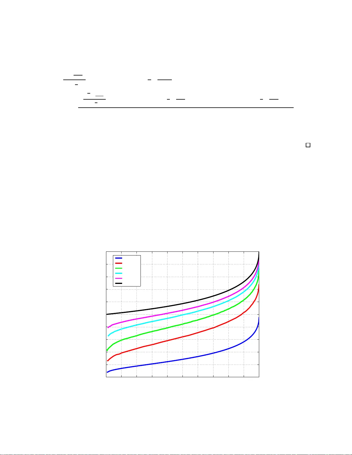
Block-len gth dependen t thresholds in block-sp arse compressed sensing M I H A I L O S T O J N I C School of Industrial Engineering Purdue Univ ersity , W est Lafa yette, IN 47907 e-mail: mstojnic@p urdue.edu July 2009 Abstract One of the most basic problems in compres sed sensing is solving an under -deter mined system of linear equati ons. Although this problem seems rather hard certain ℓ 1 -optimiz ation algorith m appears to be very succes sful in solvi ng it. The recent w ork of [1 4, 28] rigo rously prov ed (in a lar ge dimensio nal and statisti cal conte xt) that if the number of equations (measuremen ts in the compres sed sensing termino logy) in the sys- tem is pr oporti onal to the len gth of the un kno w n v ector th en there is a sp arsity (number of non -zero elements of the unkn o wn v ecto r) also propo rtional to the le ngth of the unkno wn v ector such t hat ℓ 1 -optimiz ation alg o- rithm succeed s in solving the system. In more recent papers [78, 81] we considered the setup of th e so-called block -spars e unkno wn vectors . I n a large dimensiona l and statistical conte xt, we determine d sharp lower bound s on the v alues of al lo wable spar sity for any g iv en number (proporti onal to the length of the u nkno w n vec tor) of equation s such that an ℓ 2 /ℓ 1 -optimiz ation algor ithm succe eds in solving the system. The results establ ished in [78, 81] assu med a fair ly lar ge block-le ngth of the block -spars e vectors. In this paper we c on- sider the block -length to be a para meter of the syste m. C onseq uently , we the n establish sharp lower bo unds on the v alues of the allo wable block-spars ity as functi ons of the bloc k-lengt h. Index T erms: Compress ed sensing; Block-sparse; ℓ 2 /ℓ 1 -optimizati on . 1 Introd uction In last se ve ral years the area of compress ed sensing has been the subject of ex tensi ve research . F inding the sparse st solution of an under -determined system o f lin ear equat ions turns o ut to be one of the fo cal poin ts of the entire area. R ecent phenomen al result s of [14] and [28] rig orously prov ed f or the ﬁrst time t hat in certain scenar ios one can solv e an under -determined system of linear equations by solving a linear program in polyn omial time. These break throug h results then as ex pected gen erated enor mous amount of research with possib le appli cations rangin g from high-d imension al geometry , image recons tructio n, single-p ixe l camera design , decod ing of linear codes, channel estimation in wireless communication s, to machine learning, 1 data-s treaming algorithms, DNA micro-arra ys, magneto-ence phalography etc. (more on the compressed sensin g problems, their importan ce, and wide spectrum of differ ent applica tions can be found in exce llent referen ces [4, 12, 15, 24, 37, 58, 60, 66, 68, 70, 71, 91, 93]). The interest of the present paper are the mathematical aspects of certain compres sed sensing probl ems. More precisely , we will be interested i n ﬁnding the spa rsest solution of an u nder -determined system of linear equati ons which, as mentione d abov e, is one of the most fundamenta l proble ms in the compres sed sensing. While the setu p of this problem is fa irly easy its solutio n is rather hard. Namely , the setup of the pro blem is as simple as the follo w ing: we would lik e to ﬁnd x such that A x = y (1) where A is an M × N ( M < N ) measureme nt matrix and y is an M × 1 measure ment vector . In usual compress ed sensing conte xt x is an N × 1 unkno wn K -spars e vector (see Figure 1). This assumes that x has at most K nonzero compone nts (we assume idea lly sparse si gnals; more on t he so -called approx imately sparse sign als can b e foun d in e.g. [21, 79, 84, 95]). In the rest of the p aper we will also assume the so -called linear regi me, i.e. we will assume that K = β N and that the number of the m easureme nts is M = αN where α and β are absol ute constants indepe ndent of N (more on the non-linea r reg ime, i.e. on the regime when M is lar ger than linea rly proport ional to K can be f ound in e.g. [22, 45, 46]). Since the pro blem giv en K N M = A x y Figure 1: Model of a linear system; vect or x is K -spa rse in (1) has been kno w n for a long time there is an extensi ve literatu re related to possible ways for solvin g it. If one has freedo m to design the measur ement matrix A then, clearly , a particular recov ery algo rithm for that design can be de ve loped as w ell. As sho wn in [3, 59, 65], the technique s from codin g theory (based on the coding/de coding of Reed-Solomon codes) can be employed to determine any K -sparse x in (1) for any α and any β ≤ α 2 in polynomial time. It is easy to see that β can not be greater than α 2 for x to be uniqu ely reco ver able. Therefore in terms of recov erabl e sparsity in polyn omial time results from [3, 59, 65] 2 are opti mal. The c omplex ity of algorithms from [3, 59, 65] is roughly O ( N 3 ) . If A is designed based on the techni ques related to the coding /decod ing of Expander codes then the comple xity of recov erin g x in (1) is O ( N ) (see e.g. [52, 53, 94] and referen ces therei n). Ho we ver , these algori thms do not allow for β to be as lar ge as α 2 . On the other hand, if there is no freedom in the choice of the matrix A the problem becomes NP- hard. T wo algorithms that traditio nally perform well and hav e been the subject of an extensi ve research in recent years are 1 ) Orthogo nal matchi ng pursu it - OMP and 2 ) Basis matchi ng pur suit - ℓ 1 -optimiza tion. Both of the algorithms ha ve adv antag es and disadv anta ges when applied to diffe rent problem scena rios. As exp ected a very exte nsi ve literature has been dev eloped (especial ly in last sev eral years) that cov ers vario us modiﬁcatio ns of both algorith ms so t o emphasize th eir st rength s and n eutrali ze their ﬂaws. Howe ver , a short assess ment of their dif feren ces would be that OMP is faster w hile BMP can reco v er highe r sparsity and is more resistant to system imperfections . Under certain probabil istic assumption s on the elements of the matrix A it can be sho wn (see e.g. [62, 63, 86, 88]) that if α = O ( β log ( 1 β )) OMP (or a sligh tly modiﬁed OMP) can reco ver x in (1) with comple xity of reco very O ( N 2 ) . On the other hand a stage-wise OMP from [36] reco vers x in (1) with comple xity of recov ery O ( N log N ) . Since the results of this paper wil l in some sens e be relat ed to ℓ 1 -optimiz ation (conside red in [1 4, 15, 28, 34]), below we brieﬂy recall on its deﬁnition. Basic ℓ 1 -optimiz ation algorith m (more on adapti ve versio ns of basic ℓ 1 -optimiz ation can be found in e.g. [16, 19, 76]) ﬁnds x in (1) by solv ing the follo wing problem min k x k 1 subjec t to A x = y . (2) (Instea d of ℓ 1 -optimiz ation one can employ ℓ q -optimiz ation, 0 < q < 1 , which essentiall y me ans that instead of norm 1 one c an use norm q in (1). Howe ver the resu lting pr oblem becomes non-co n vex . A good ov ervie w of that approac h can be found in e.g. [26, 43, 48–50, 75] and refere nces therei n.) Quite remarkab ly , in [15] the author s were able to sho w that i f α and N are gi ven , the matrix A is gi ven and satisﬁes a special p ropert y called the restri cted isometry property (RIP), then any unkno w n vector x with no more than K = β N (where β is an absolute cons tant dependent on α and expl icitly calculated in [15]) non-zero element s can be reco ver ed by solving (2). As expected , this assumes that y was in fact gene rated by that x and gi ve n to us. The case when th e a v ailable measuremen ts are noisy vers ions of y is also of interes t [14, 15, 51, 92]. W e mention in passing that the recent popu larity of ℓ 1 -optimiz ation in compresse d sensing is signiﬁcantly due to its robu stness with respec t to noisy measurements. (Of course, the main reaso n for its popularity is its 3 ability to solve (1) for a ve ry wide range of matrices A ; more on this remarkabl e uni v ersality phenomen on the interes ted reader can ﬁnd in [33].) Since the RIP condit ion played a crucial role in proving technique of [14, 15] hav ing the matrix A satisfy the RIP conditio n is fundamentall y importan t. (More on the importanc e of the RIP condition can be foun d in [13]). Design ing determini stic matrices for which the R IP condi tion would hold as well as checki ng if it holds for any giv en matrix is a v ery hard proble m. Ho we ver , for se ve ral class es of rando m matrices (e.g., matr ices with i.i.d. zero m ean Gaussian, Berno ulli or ev en general Sub-gauss ian co mponent s) it turns out that for certain dimension s of the system the RIP condi tion is satisﬁed with overwhe lming probab ility [1, 5, 15, 73]. O n the other hand, it should also be pointed out that the RIP is only a sufﬁc ient condit ion for ℓ 1 -optimiz ation to produce the solution of (1). In turn this means that an analys is of ℓ 1 - optimiza tion success is not requir ed to rely on it. In fa ct, the ﬁnal results and brilliant analysis of [27, 28] do not rely on the v alidity of the RIP cond ition. Namely , in [27, 28] the author consi ders polyt ope obtained by projecting the regula r N -dimensional cross- polyto pe using the matrix A . It turns out that a necessa ry and sufﬁ cient condi tion for (2) to produc e the soluti on of (1) for any giv en x is that this polytope associated with the matrix A is K -neig hborly [27–30]. Using the results of [2, 10, 72, 90], it is further sho wn in [28], that if the matrix A is a random m × n ortho- project or matrix then with ov erwhelmin g probability poly tope obtained projecting the stand ard N - dimensio nal cross-po lytope by A is K -neighb orly . The precis e relation between M and K in order for this to happ en is charac terized in [27, 28] as well. It shou ld be noted that one usually considers success of (2) in ﬁnding solution of (1) for any gi ven x . It is also of interest to consider success of (2) in ﬁ nding soluti on of (1) for almost any giv en x . T o make a distin ction between these two cases we will in the follo wing section recall on sev eral important deﬁnitions from [28, 29, 31]. Before proceed ing furthe r we ﬁrst in the follo wing section introduce the so-called block-spar se signals that will be the ce ntral topic of this paper . Immediately afterw ards we also describ e a polynomial algorithm for their ef ﬁcient reco ve ry . 2 Block-sparse signals and ℓ 2 /ℓ 1 -algorithm What we described in the pre vious sectio n is the standard compres sed sensin g setup. Such a setup does not assume any special struct ure on the unkno w n K -spars e signal x . Howe ver one may encounter applicatio ns when the signal x in add ition to being sparse has a certain structu re. T he so-called blo ck-spar se signals were 4 introd uced and its a pplicat ions and reco ver y algori thms were in ves tigated in [4 , 17, 38– 40, 44, 65, 78, 81, 83]. A related pro blem of reco veri ng jo intly sparse signals and its applicat ions were considered in [6, 9, 18, 23, 41, 61, 64, 85, 87, 89, 91, 97, 98] and referen ces therein ( more on d if ferent t ypes of a priori kn o wn si gnal stru cture can also be found in [55, 56, 96]). In all these cases one attempts to improv e the reco v erabilit y potential of the standard algorithms described in the pre vious section by incorporatin g the knowled ge of the signal structu re. In this paper we will be interest ed in f urther in vestig ating the so-cal led block-s parse compre ssed sen sing proble ms [4, 40, 65, 78, 81, 83]. T o intro duce block-spars e signals and fa cilitate the subsequ ent exposit ion we w ill assume that integers N and d are chosen such that n = N d is an integ er and it represents the total number of blocks that x cons ists of. Clearly d is the length of each block. Furthermore, we will assume that m = M d is an integer as well and that X i = x ( i − 1) d +1: id , 1 ≤ i ≤ n are the n blocks of x (see Figure 2). Then we will call any signal x k-block-spa rse if its at most k = K d blocks X i are non-zero (non-zero x 1 x id − d +1 x id − d +2 x id x nd − d +2 X i x 2 x d x nd − d +1 X n x nd X 1 y . . . . . . . . . } } } . . . . . . A 1 A n A i A 1 — columns 1 , 2 , . . . , d A i — columns id − d + 1 , id − d + 2 , . . . , id A n — columns nd − d + 1 , nd − d + 2 , . . . , nd = . . . y = A x = P n i =1 A i X i . . . Figure 2: Block-spa rse model block is a block that is not a zero block; zero block is a block that has all elements equal to zero) . S ince k -block-s parse signals are K -spa rse one could then use (2) to recov er the solution of (1). While this is possib le, it clear ly uses the block structu re of x in no way . T o exp loit the block structure of x in [83] the follo wing polynomial algorithm (essen tially a combination of ℓ 2 and ℓ 1 optimiza tions) was consi dered (see 5 also e.g. [4, 39, 89, 97, 98]) min n X i =1 k x ( i − 1) d +1: id k 2 subjec t to A x = y . (3) Extensi ve s imulation s in [83] demonstra ted that as d grows the a lgorith m in (3) signiﬁcantl y out performs th e standa rd ℓ 1 . The follo w ing was sho wn in [83] as well: let A be an M × N matrix with a ba sis of nul l-space comprise d of i.i.d. Gaussian elements; if α = M N → 1 then there is a consta nt d such that al l k -block-s parse signal s x with sparsity K ≤ β N , β → 1 2 , can be recov ered with ov erwhel ming probability by solvin g (3). The precise relati on between d and how fast α − → 1 and β − → 1 2 was quant iﬁed in [83] as well. In [78, 81] we extended the results from [83] and obtain ed the va lues of the recov erable block -sparsi ty for any α , i.e. for 0 ≤ α ≤ 1 . More precisely , for any giv en constant 0 ≤ α ≤ 1 we in [78, 81] determined a constant β = K N such that for a suf ﬁciently lar ge d (3) with ove rwhelming probab ility recov ers any k -block- sparse signal with sparsity less then K . (Und er over whelming probability we in this paper assume a prob ability that is no more than a number ex ponent ially decaying in N awa y from 1 .) Clearly , for any gi ven constan t α ≤ 1 there is a maximum allo wabl e val ue of the cons tant β such that (3) ﬁnds solut ion of (1) with ov erwhelmin g probabili ty for any x . This maximum allo wabl e valu e of the consta nt β is called the str ong thr eshold (see [27, 28]). W e will denote the va lue of the strong thresho ld by β s . S imilarly , f or any giv en constant α ≤ 1 one can deﬁne the sectional thr eshold as the ma ximum allo wable v alue of the constant β such that (3) ﬁnds the soluti on of (1) with ov erwhelming probabilit y for any x with a gi ven ﬁ xed locati on of non-zer o blocks (see [27, 28]). In a similar fash ion one can then denote the v alue of the sectional thresh old by β sec . Finally , for any giv en constant α ≤ 1 one can deﬁne the weak thr eshold as the maxi mum allo wable v alue of the constan t β such that (3) ﬁnds the s olution of (1) with o v erwhelming probab ility for any x with a giv en ﬁ xed location of non-zero blocks and giv en ﬁxed directions of non-zero block vect ors X i (see [27, 28]). In a similar fashi on one can then denote the value of the weak thresh old by β w . While [78, 81] provide d fairly sharp thresho ld v alues the y had done so in a some w hat asymptot ic sense. Namely , the analysi s p resent ed in [78, 81] ass umed fairl y lar ge v alues of block- length d . As such the analys is in [78, 81] then provid ed an ultimate performance limit of ℓ 2 /ℓ 1 -optimiz ation rather than its performanc e charac terizati on as a function of a particu lar ﬁxed block-lengt h. In this paper we extend the results from [78, 81] so that the thres hold values are no w func tions of a ﬁxed block-leng th d . Our analys is w ill use some ingredient s of the analysis presented in [78, 81]. Ho w e ver , signiﬁcantly more precise estimates of 6 certain quantities will be necessa ry to accoun t for a ﬁxed block-leng th. These estimates will be obtaine d in a fashion similar to the one presented in [82]. In addition to the strong threshol ds (which w ere the main concern of [78, 81]), we will also determine attaina ble val ues for the section al and weak threshol ds as functi ons of a ﬁxed blo ck-len gth d for the entire range of α , i.e. for an y 0 < α ≤ 1 . W e or ganiz e the rest of the pa per in the f ollo w ing way . In Section 3 we introdu ce two k ey theorems that will be the heart of our subsequ ent analys is. In Section 4 we determine the value s of the strong, sectio nal, and w eak thresho lds for a gi ven block-len gth d under the assumptio n that the null-spac e of the matrix A is uniformly distrib uted in the G rassmani an. In Section 5 we determine the asymptot ic value s of the strong , sectional, and weak threshold s assuming large block length d . In S ection 6 we present the resu lts of the conducted numerical experi ments and ﬁ nally , in S ection 7 we discuss obtained results and possibl e directi ons for future work. 3 Null-space and escape through a mesh theor ems In this sectio n we introduce two useful theor ems that will be of ke y importance in our subsequent analysis . First we recall on a null-space characte rizatio n of the matrix A w hich establish es a guarant ee that the solu- tions of (1) and (3) coincide. The follo wing theorem from [78, 81, 83] provide s this characteriz ation. S et K to be the set of all subsets of size k of { 1 , 2 , . . . , n } ; also if κ ⊂ K then κ c = { 1 , 2 , . . . , n } \ κ . Theor em 1. ( [83]) Assume that A is a dm × dn measur ement m atrix, y = A x and x is k -bloc k-sparse . Then the solutio ns of (3) and (1) coinside if and only if for all nonzer o w ∈ R dn wher e A w = 0 and all κ ∈ K X i ∈ κ || W i || 2 < X i ∈ κ c || W i || 2 (4) wher e W i = ( w ( i − 1) d +1 , w ( i − 1) d +2 , . . . , w id ) T , i = 1 , 2 , . . . , n . The follo wing three remarks seem to be in order . Remark 1: The follo wing simpliﬁcation of the pre vious theorem is also well-kno wn. Let w ∈ R n be such that A w = 0 . Further , let W ( norm ) = ( k W 1 k 2 , k W 2 k 2 , . . . , k W n k 2 ) T and let | W ( norm ) | ( i ) be the i -th smallest of the elements of W ( norm ) . Set ˜ W = ( | W ( norm ) | (1) , | W ( norm ) | (2) , . . . , | W ( norm ) | ( n ) ) T . If ( ∀ w | A w = 0) P n i = n − k +1 ˜ W i ≤ P n − k i =1 ˜ W i , where ˜ W i is the i -th element of ˜ W , then the solutions of (1) and (3) coincid e. Remark 2: Characteriza tion giv en in the pre vious theorem (and prov en in [83]) is a mere analogue to the simila r characteriz ations related to the equ iv alence of (1) and (2) from e.g. [32 , 35, 42, 57, 80, 83, 95, 99]. 7 If instead of ℓ 1 one, for example, uses an ℓ q -optimiz ation ( 0 < q < 1 ) in (2) then chara cteriza tions similar to the ones from [32, 35, 42, 57, 83, 95, 99] can be deri ved as w ell [48– 50]. In a similar fashion one could then deri ve an equ iv alent to the pre vious theorem for the ℓ 2 /ℓ q -optimiz ation, 0 < q < 1 . Remark 3: Checking if the cond ition gi ven in the abov e theor em is satisﬁed for a gi ven matrix A is a ver y importan t a nd difﬁcult problem. Although it is not the main topic of the presen t p aper , we do mention in passin g that a po ssible approxi mate way of s olving it wo uld be a gene ralizati on of resul ts from e.g. [2 5, 54]. Clearly , if one can cons truct the m atrix A such that (4) holds then the solution of (3) would be the soluti on of (1). If one a ssumes that m and k are proport ional to n (the cas e of ou r inte rest in thi s pap er) then the construc tion of the determini stic matrices A that would satisfy (4) is not an easy task. Howe v er , if one turns to random matrices this appears to be signiﬁcant ly easier . In the following sections we will show that this is indee d possibl e for a partic ular type of rando m matrices. More precise ly , as we hav e already hinted earlier , we will consider the random matrices A that hav e the null-s pace unifor mly distrib uted in the Grassmanian. The follo wing phenomenal result from [47] that relates to such matrices will be one of ke y ingre dients in the analy sis that will follo w . Theor em 2. ( [47] Escape thr ough a mesh) Let S be a subset of the unit Euclidean spher e S dn − 1 in R dn . Let Y be a ra ndom d ( n − m ) -dimensio nal subspace of R dn , distr ib uted unifor mly in the Grassmania n with r espect to the Haar measur e. Let w ( S ) = E sup w ∈ S ( h T w ) (5) wher e h is a rand om column vector in R dn with i.i.d. N (0 , 1) component s, w is a dn -dimension al column vector fr om S , and h T is the tra nspose of h . A ssume that w ( S ) <  √ dm − 1 4 √ dm  . Then P ( Y ∩ S = 0) > 1 − 3 . 5 e − „ √ dm − 1 4 √ dm − w ( S ) « 2 18 . (6) Remark : Gordon’ s origi nal consta nt 3 . 5 was substitu ted by 2 . 5 in [74]. B oth constants are ﬁne for our subseq uent analys is. 4 Pr obabilistic analysis of the null-space characterizations In this section we probabilisti cally analyze v alidity of the null-s pace characteriz ation gi ve n in Theorem 1. In the ﬁrst subsection of this section we w ill sho w how one can obtain the valu es of the strong threshold β s for the entire range 0 ≤ α ≤ 1 based on such an analysis. In the later two subsec tions we w ill extend the 8 strong thresh old analy sis and obtain the v alues of the section al and w eak thresh olds. 4.1 Str ong thr eshold As master ly noted in [74] Theorem 2 can be used to p robab ilistica lly analyze (4) (and as we will s ee lat er in the paper , many o f its v ariants ). Namely , let S in (5) be S s = { w ∈ S dn − 1 | n X i = n − k +1 ˜ W i ≤ n − k X i =1 ˜ W i } (7) where as earlier the notatio n ˜ W is used to denote the vecto r obtained by sorting the element s of W ( norm ) in non-de creasin g order (esse ntially , ˜ W is a ve ctor obtained by sorting magnitudes of blocks W i in non- decrea sing order). A lso, here and in an analogou s fashion in the later sections of the paper , we assume that k is suc h that there is a n α , 0 < α ≤ 1 , such that the so lution s of (1) an d (3) coin cide. L et Y be a d ( n − m ) dimensio nal subspa ce of R dn unifor mly distrib uted in Gras smanian. Furthermore, le t Y be th e n ull-spa ce of A . Then as long as w ( S s ) <  √ dm − 1 4 √ dm  , Y will miss S s (i.e. (4) wil l b e sati sﬁed) with p robabi lity no smaller than the one gi ve n in (6). More precisely , if α = m n is a constant (the case of interest in this paper) , n, m are lar ge, and w ( S s ) is smalle r than b ut proport ional to √ dm then P ( Y ∩ S s = 0) − → 1 . This in tur n is equi valen t to hav ing P ( ∀ w ∈ R dn | A w = 0 , n X i = n − k +1 ˜ W i ≤ n − k X i =1 ˜ W i ) − → 1 which accord ing to Theorem 1 (or more precisely accordin g to remark 1 after T heorem 1) means that the soluti ons of (1) and (3) coincide with probability 1 . For an y gi ven valu e of α ∈ (0 , 1) a thresh old v alue of β can then be determined as a maximum β such that w ( S s ) <  √ dm − 1 4 √ dm  . That maximum β w ill be exactly the va lue of the strong threshol d β s . If one is only concerned with ﬁnding a possib le v alue for β s it is easy to note that instead of computi ng w ( S s ) it is sufﬁcien t to ﬁnd its an upper bound. Ho wev er , to determin e as good v alues of β s as possible, the upper bound on w ( S s ) should be as tight as possibl e. The main contrib ution of this work will be a fairl y precise estimate of w ( S s ) . In the f ollo w ing subsec tions we present a way to get such an e stimate. T o simplify the expositio n we ﬁrst set w ( h , S s ) = max w ∈ S s ( h T w ) . In o rder to upper -bound w ( S s ) we will ﬁrst in S ubsect ion 4.1.1 determin e an upper bound B s on w ( h , S s ) . The expe cted va lue with respect to h of such an upper bound will be an upper bou nd on w ( S s ) . In Subs ection 4.1.2 we wil l compu te an upp er bound on th at ex pected v alue , i.e. we will compute an uppe r boun d on E ( B s ) . That quant ity will be an uppe r boun d on w ( S s ) since accord ing to 9 the follo w ing E ( B s ) is an upper bound on w ( S s ) w ( S s ) = E w ( h , S s ) = E ( max w ∈ S s ( h T w )) ≤ E ( B s ) . (8) 4.1.1 Upper -bounding w ( h , S s ) Let H i = ( h ( i − 1) d +1 , h ( i − 1) d +2 , . . . , h id ) T , i = 1 , 2 , . . . , n . From the deﬁnition of set S s gi ve n in (7) it easily follows that if w is in S s then an y vec tor obtain from w by rotating (essenti ally multip lying by orthog onal matrices) any subset of its blocks W i , 1 ≤ i ≤ n , in any direct ion is also in S s . The directions of vecto rs W i , 1 ≤ i ≤ n , can therefo re be chosen so that they match the directions of vecto rs H i , 1 ≤ i ≤ n of the corres pondin g block s in h . W e then easily ha ve w ( h , S s ) = m ax w ∈ S s ( h T w ) = max w ∈ S s n X i =1 | h i w i | = max w ∈ S s n X i =1 k H i k 2 k W i k 2 . (9) Let H ( norm ) = ( k H 1 k 2 , k H 2 k 2 , . . . , k H n k 2 ) . Further , let | H ( norm ) | ( i ) be the i -th smalles t of the elements of H ( norm ) . S et ˜ H = ( | H ( norm ) | (1) , | H ( norm ) | (2) , . . . , | H ( norm ) | ( n ) ) T . If w ∈ S s then a vecto r obtain ed by permutin g the block s of w in any possible way is also in S s . Then (9) can be rewri tten as w ( h , S s ) = m ax w ∈ S s n X i =1 ˜ H i k W i k 2 (10) where ˜ H i is the i -th element of vector ˜ H . Let ˆ w be the solution of the maximizatio n on the right-ha nd si de of (10). Further let ˆ W i = ( ˆ w ( i − 1) d +1 , ˆ w ( i − 1) d +2 , . . . , ˆ w id ) T , i = 1 , 2 , . . . , n . It then easily follo w s k ˆ W n k 2 ≥ k ˆ W n − 1 k 2 ≥ k ˆ W n − 2 k 2 ≥ · · · ≥ k ˆ W 1 k 2 . T o see this assume that there is a pair of inde xes n 1 , n 2 such that n 1 < n 2 and k ˆ W n 1 k 2 > k ˆ W n 2 k 2 . H o wev er , k ˆ W n 1 k 2 ˜ H n 1 + k ˆ W n 2 k 2 ˜ H n 2 < k ˆ W n 2 k 2 ˜ H n 1 + k ˆ W n 1 k 2 ˜ H n 2 and ˆ w wou ld not be the optimal solution of the maximization on the right-ha nd side of (10). Let y = ( y 1 , y 2 , . . . , y n ) T ∈ R n . Then one can simplify (10) in the follo wing way w ( h , S s ) = max y ∈ R n n X i =1 ˜ H i y i subjec t to y i ≥ 0 , 0 ≤ i ≤ n n X i = n − k +1 y i ≥ n − k X i =1 y i n X i =1 y 2 i ≤ 1 . (11) 10 One can add the sort ing constrai nts on the elements of y in the optimiza tion problem abov e. H o wev er , the y would be redunda nt, i.e. any solution ˆ y to the above optimization problem will automat ically satisfy ˆ y n ≥ ˆ y n − 1 ≥ · · · ≥ ˆ y 1 . T o determine an upper bound on w ( h , S s ) we will use the method of Lagrange dualit y . The deri vatio n of Lagran ge dual up per bou nd will closely foll o w a similar deri vati on from [8 2]. For the complet eness we reprod uce it here as w ell. Before deri ving the Lagrange dual we slightly modify (11) in the follo wing way − w ( h , S s ) = min y ∈ R n − n X i =1 ˜ H i y i subjec t to y i ≥ 0 , 0 ≤ i ≤ n n X i = n − k +1 y i ≥ n − k X i =1 y i n X i =1 y 2 i ≤ 1 . (12) T o further fac ilitate writing let z ∈ R n be a column vecto r such that z i = 1 , 1 ≤ i ≤ ( n − k ) and z i = − 1 , n − k + 1 ≤ i ≤ n . Further , let λ = ( λ 1 , λ 2 , . . . , λ n ) T ∈ R n . Follo w ing, e.g. [11], w e can write the dual of the optimiz ation proble m (12) and its optima l v alue w up ( h , S s ) as − w up ( h , S s ) = max γ ,ν ,λ min y − ˜ H T y + γ || y || 2 2 − γ + ν z T y − λ T y subjec t to ν ≥ 0 , γ ≥ 0 λ i ≥ 0 , 0 ≤ i ≤ n. (13) One can then trans form the objec ti ve function in the follo wing way − w up ( h , S s ) = max γ ,ν ,λ min y k √ γ y − λ + ˜ H − ν z 2 √ γ k 2 2 − γ − k λ + ˜ H − ν z k 2 2 4 γ subjec t to ν ≥ 0 , γ ≥ 0 λ i ≥ 0 , 0 ≤ i ≤ n. (14) After tri vially solving the inner minimization in (14) we obtain w up ( h , S s ) = min γ ,ν ,λ γ + k λ + ˜ H − ν z k 2 2 4 γ subjec t to ν ≥ 0 , γ ≥ 0 λ i ≥ 0 , 0 ≤ i ≤ n. (15) 11 Minimizati on ov er γ is straightf orward and one easily o btains t hat γ = k λ + ˜ H − ν z k 2 2 is optimal. Plugging t his v alue of γ back in the objec ti ve function of the optimization problem (15) one obtains w up ( h , S s ) = min ν,λ k λ + ˜ H − ν z k 2 subjec t to ν ≥ 0 λ i ≥ 0 , 0 ≤ i ≤ n. (16) By d uality , − w up ( h , S s ) ≤ − w ( h , S s ) w hich easily implies w ( h , S s ) ≤ w up ( h , S s ) . Therefore w up ( h , S s ) is an upper bound on w ( h , S s ) . (In fact one can easily s ho w that the strong duality holds and that w ( h , S s ) = w up ( h , S s ) ; ho we ve r , as exp lained earlier , for our analysis sho wing that w up ( h , S s ) is an uppe r bound on w ( h , S s ) is sufﬁcien t.) Along the same lines , one can easily spot that an y feasible v alues ν and λ in (16) will provide a val id up per b ound on w up ( h , S s ) and hence a v alid upper b ound on w ( h , S s ) . In what follows we will in fact determine the optimal val ues for ν and λ . Howe ver , since it is not necessary for our analysis we will not p ut too much ef fort into provi ng that these v alues are optimal . As we ha ve stat ed earlier , for our analys is it will be enough to sho w that the va lues for ν and λ that we will obtain are feasible in (16) . T o facilitate the expositio n in what follo ws instead of dealing with the objecti ve function giv en in (16) we will be deali ng with its squared v alue . Hence, we set f ( h , ν , λ ) = k λ + ˜ H − ν z k 2 2 . No w , let λ = ( λ 1 , λ 2 , . . . , λ c , 0 , 0 , . . . , 0) T , λ 1 ≥ λ 2 ≥ · · · ≥ λ c ≥ 0 where c ≤ ( n − k ) is a crucial parameter that will be determine d later . The optimizat ion ov er ν in (16) is then seemin gly strai ghtforw ard. S etting the deri vati ve of f ( h , ν, λ ) with res pect to ν to zero we ha ve d k λ + ˜ H − ν z k 2 2 dν = 0 ⇔ − 2( λ + ˜ H ) T z + 2 k z k 2 2 ν = 0 ⇔ ν = ( λ + ˜ H ) T z k z k 2 2 . (17) If ( λ + ˜ H ) T z ≥ 0 then ν = ( λ + ˜ H ) T z k z k 2 2 is inde ed the optimal in (16). For the time being let us assume that λ, h , c are such that ν = ( λ + ˜ H ) T z k z k 2 2 ≥ 0 . For ν = ( λ + ˜ H ) T z k z k 2 2 we ha ve f ( h , ( λ + ˜ H ) T z k z k 2 2 , λ ) = k ( λ + ˜ H ) T ( I − zz T z T z ) k 2 2 = ( λ + ˜ H ) T ( I − zz T z T z )( λ + ˜ H ) . (18) 12 Simplifying (18) furth er w e obtain f ( h , ( λ + ˜ H ) T z k z k 2 2 , λ ) = n X i =1 ˜ H 2 i + 2 c X i =1 λ i ˜ H i + c X i =1 λ 2 i − ( ˜ H T z ) 2 n − ( P c i =1 λ i ) 2 n − 2( P c i =1 λ i )( ˜ H T z ) n . (19) T o determine good v alues for λ w e proceed by setting the deri v ati ves of f ( h , ( λ + ˜ H ) T z k z k 2 2 , λ ) with respect to λ i , 1 ≤ i ≤ c to zero d f ( h , ( λ + ˜ H ) T z k z k 2 2 , λ ) dλ i = 2 λ i + 2 ˜ H i − 2 ( P c i =1 λ i ) n − 2 ( ˜ H T z ) n = 0 . (20) Summing the abo ve deri vati ves ov er i and equalling w ith zero we obtain c X i =1 d f ( h , ( λ + ˜ H ) T z k z k 2 2 , λ ) dλ i = 2( c X i =1 λ i + c X i =1 ˜ H i − c ( P c i =1 λ i ) n − c ( ˜ H T z ) n ) = 0 . (21) From (21) one then easily ﬁnds c X i =1 λ i = c ( ˜ H T z ) n − c − n P c i =1 ˜ H i n − c . (22) Plugging the v alue for P c i =1 λ i obtain ed in (22) in (20) we ha ve λ i = ( ˜ H T z ) n − ˜ H i + ( P c i =1 λ i ) n = ( ˜ H T z ) n − ˜ H i + c ( ˜ H T z ) n ( n − c ) − P c i =1 ˜ H i n − c and ﬁnally λ i = ( ˜ H T z ) − P c i =1 ˜ H i n − c − ˜ H i , 1 ≤ i ≤ c λ i = 0 , c + 1 ≤ i ≤ n. (23) Combining (17) and (22) we ha ve ν = ( λ + ˜ H ) T z k z k 2 2 = ˜ H T z + P c i =1 λ i n = ˜ H T z + c ( ˜ H T z ) n − c − n P c i =1 ˜ H i n − c n = ( ˜ H T z ) − P c i =1 ˜ H i n − c . (24) From (23) we then ha ve as ex pected ν = λ i + ˜ H i , 1 ≤ i ≤ c. (25) As long as we can ﬁnd a c such that λ i , 1 ≤ i ≤ c giv en in (23) are non-ne gati ve ν will be non-ne gativ e as 13 well and ν and λ will therefore be feasible in (16). This in turn implies w ( h , S s ) ≤ p f ( h , ν, λ ) (2 6) where f ( h , ν, λ ) is computed for the va lues of λ and ν gi v en in (23) and (25), respecti vely . (In fact deter - mining the larges t c such that λ i , 1 ≤ i ≤ c gi ven in (23) are non-ne gati v e will insure that p f ( h , ν, λ ) = w ( h , S s ) ; ho we ve r , as already stated earlier , this fac t is not of any speci al importance for our analys is). Let us now assu me that c is ﬁ xed such that λ and ν are as giv en in (23) and (25). Then combining (19), (22), and (25) we ha ve f ( h , ( λ + ˜ H ) T z k z k 2 2 , λ ) = n X i =1 ˜ H 2 i + 2 ν c X i =1 ˜ H i − 2 c X i =1 ˜ H 2 i + cν 2 − 2 ν c X i =1 ˜ H i + c X i =1 ˜ H 2 i − ( P c i =1 λ i + ˜ H T z ) 2 n . (27) Combining (22) and (24) we obtain ( c X i =1 λ i + ˜ H T z ) = nν. (28) Further , combining (27) and (28) we ﬁnd f ( h , ( λ + ˜ H ) T z k z k 2 2 , λ ) = n X i =1 ˜ H 2 i + cν 2 − c X i =1 ˜ H 2 i − ( nν ) 2 n = n X i =1 ˜ H 2 i + ( c − n ) ν 2 − c X i =1 ˜ H 2 i = n X i =1 ˜ H 2 i − c X i =1 ˜ H 2 i − (( ˜ H T z ) − P c i =1 ˜ H i ) 2 n − c . (29) Finally , combining (26) and (29) we ha v e w ( h , S s ) ≤ v u u t n X i =1 ˜ H 2 i − c X i =1 ˜ H 2 i − (( ˜ H T z ) − P c i =1 ˜ H i ) 2 n − c = v u u t n X i = c +1 ˜ H 2 i − (( ˜ H T z ) − P c i =1 ˜ H i ) 2 n − c . (30) Clearly , as long as ( ˜ H T z ) ≥ 0 there will be a c ≤ n − k (it is poss ible that c = 0 ) such that quantity on the most right hand side of (30) is an upper bound on w ( h , S s ) . T o facil itate the exposit ion in the followin g subsection we will make the upper boun d giv en in (30) slight ly more pessimis tic in the follo wing lemma. Lemma 1. Let h ∈ R dn be a vector w ith i.i.d. zer o-mean unit variance gaus sian components. Let H i = ( h ( i − 1) d +1 , h ( i − 1) d +2 , . . . , h id ) T , i = 1 , 2 , . . . , n and H ( norm ) = ( k H 1 k 2 , k H 2 k 2 , . . . , k H n k 2 ) . Furth er , 14 let | H ( norm ) | ( i ) be the i -th smalles t of the element s of H ( norm ) . Set ˜ H = ( | H ( norm ) | (1) , | H ( norm ) | (2) , . . . , | H ( norm ) | ( n ) ) T and w ( h , S s ) = max w ∈ S s ( h T w ) wher e S s is as deﬁne d in (7). L et z ∈ R n be a column vector suc h that z i = 1 , 1 ≤ i ≤ ( n − k ) and z i = − 1 , n − k + 1 ≤ i ≤ n . Then w ( h , S s ) ≤ B s (31) wher e B s =      q P n i =1 ˜ H 2 i if ζ s ( h , c s ) ≤ 0 q P n i = c s +1 ˜ H 2 i − (( ˜ H T z ) − P c s i =1 ˜ H i ) 2 n − c s if ζ s ( h , c s ) > 0 , (32) ζ s ( h , c ) = ( ˜ H T z ) − P c i =1 ˜ H i n − c − ˜ H c and c s = δ s n is a c ≤ n − k such that (1 − ǫ ) E (( ˜ H T z ) − P c i =1 ˜ H i ) n − c − F − 1 χ d  (1 + ǫ ) c n  = 0 . (33) F − 1 χ d ( · ) is the in vers e cdf of the chi random variable with d de gr ees of free dom, i.e. it is the in verse cdf of random variab le q P d i =1 Z 2 i wher e Z i , 1 ≤ i ≤ d ar e indepe ndent zer o-mean , unit variance G aussia n ran dom variable s. ǫ > 0 is an arbitrar ily small constan t indepen dent of n . Pr oof. Follo ws from the pre vious analys is and (30). 4.1.2 Computing an upper bound on E ( B s ) In th is subsectio n we will compute an upper boun d on E ( B s ) . Again, the deri v ation will closel y follo w that of [82]. (Ho we ver , due to a fe w block-stru cture related dif feren ces in the der i v ations of Lemmas 2 and 3 we includ e it here.) As a ﬁrst step we determin e a lower bou nd on P ( ζ s ( h , c s ) > 0) . W e start by a sequen ce of obv ious inequali ties P ( ζ s ( h , c s ) > 0) ≥ P ζ s ( h , c s ) ≥ (1 − ǫ ) E (( ˜ H T z ) − P c s i =1 ˜ H i ) n − c s − F − 1 χ d  (1 + ǫ ) c s n  ! ≥ P (( ˜ H T z ) − P c s i =1 ˜ H i ) n − c s ≥ (1 − ǫ ) E (( ˜ H T z ) − P c s i =1 ˜ H i ) n − c s and F − 1 χ d  (1 + ǫ ) c s n  ≥ ˜ H c s ! ≥ 1 − P (( ˜ H T z ) − P c s i =1 ˜ H i ) n − c s < (1 − ǫ ) E (( ˜ H T z ) − P c s i =1 ˜ H i ) n − c s ! − P  F − 1 χ d  (1 + ǫ ) c s n  < ˜ H c s  (34) 15 The rest of the analy sis assumes that n is lar ge so that δ s can be assumed to be real (of cour se, δ s is a propo rtionali ty constant indep endent of n ). Using the result s from [7] we obtain P  F − 1 χ d  (1 + ǫ ) c s n  < ˜ H c s  ≤ exp ( − n 2 (1+ ǫ ) c s n  c s n − (1 + ǫ ) c s n  2 ) ≤ exp  − nǫ 2 δ s 2(1 + ǫ )  . (35) W e will also n eed t he follo wing brilliant r esult from [ 20]. Let ξ ( · ) : R dn − → R be a Lipschitz functio n such that | ξ ( a ) − ξ ( b ) | ≤ σ k a − b k 2 . Let a be a vec tor comprised of i.i.d. zero- mean, unit varian ce Gaussian random v ariab les. Then P ((1 − ǫ ) E ξ ( a ) ≥ ξ ( a )) ≤ exp  − ( ǫE ξ ( a )) 2 2 σ 2  . (36) Let ξ ( h ) = ( ˜ H T z ) − P c s i =1 ˜ H i . T he follo wing lemma estimates σ (for simplicity w e assume c s = 0 ; the proof easily ex tends to the case when c s 6 = 0 ). Lemma 2. Let a , b ∈ R dn . L et A i = ( a ( i − 1) d +1 , a ( i − 1) d +2 , . . . , a id ) and B i = ( b ( i − 1) d +1 , b ( i − 1) d +2 , . . . , b id ) , i = 1 , 2 , . . . , n . Set A ( norm ) = ( k A 1 k 2 , k A 2 k 2 , . . . , k A n k 2 ) and B ( norm ) = ( k B 1 k 2 , k B 2 k 2 , . . . , k B n k 2 ) . Further , let | A ( norm ) | ( i ) , | B ( norm ) | ( i ) be the i -th smalles t of the elemen ts of A ( norm ) , B ( norm ) , r espectiv ely . Set ˜ A = ( | A ( norm ) | (1) , | A ( norm ) | (2) , . . . , | A ( norm ) | ( n ) ) T and ˜ B = ( | B ( norm ) | (1) , | B ( norm ) | (2) , . . . , | B ( norm ) | ( n ) ) T . Then | ξ ( a ) − ξ ( b ) | = | n − k X i =1 ˜ A i − n X n − k +1 ˜ A i − n − k X i =1 ˜ B i + n X n − k +1 ˜ B i | ≤ √ n v u u t dn X i =1 | a i − b i | 2 = √ n k a − b k 2 . (37) Pr oof. W e ha v e | n − k X i =1 ˜ A i − n X i = n − k +1 ˜ A i − n − k X i =1 ˜ B i + n X i = n − k +1 ˜ B i | ≤ | n − k X i =1 ( ˜ A i − ˜ B i ) | + | n X i = n − k +1 ( ˜ A i − ˜ B i ) | ≤ n − k X i =1 | ˜ A i − ˜ B i | + n X i = n − k +1 | ˜ A i − ˜ B i | ≤ n X i =1 | ˜ A i − ˜ B i | ≤ √ n v u u t n X i =1 | ˜ A i − ˜ B i | 2 ≤ √ n v u u t n X i =1 | ˜ A i | 2 + n X i =1 | ˜ B i | 2 − 2 n X i =1 ˜ A i ˜ B i = √ n v u u t dn X i =1 | a i | 2 + dn X i =1 | b i | 2 − 2 n X i =1 ˜ A i ˜ B i . (38) 16 Since the componen ts of ˜ A and ˜ B are positi v e and sorted in the same non-decre asing order we hav e n X i =1 ˜ A i ˜ B i ≥ n X i =1 k A i k 2 k B i k 2 . (39) By Cauchy-Sch wartz inequali ty we hav e n X i =1 k A i k 2 k B i k 2 ≥ n X i =1 d X j =1 a ( i − 1) d + j b ( i − 1) d + j = dn X i =1 a i b i . (40) From (39) and (40) we obtain − n X i =1 ˜ A i ˜ B i ≤ − dn X i =1 a i b i . (4 1) Combining (38) and (41) we ﬁnally ha ve | n − k X i =1 ˜ A i − n X i = n − k +1 ˜ A i − n − k X i =1 ˜ B i + n X i = n − k +1 ˜ B i | ≤ √ n v u u t dn X i =1 | a i | 2 + dn X i =1 | b i | 2 − 2 n X i =1 ˜ A i ˜ B i ≤ √ n v u u t dn X i =1 | a i | 2 + dn X i =1 | b i | 2 − 2 dn X i =1 a i b i = √ n v u u t dn X i =1 | a i − b i | 2 . (42) Connecti ng beg inning and end in (42) establishe s (37). For ξ ( h ) = ( ˜ H T z ) − P c s i =1 ˜ H i the pre vious lemma then giv es σ ≤ √ n (in fac t if there was n o assump- tion that c s = 0 one would rather handily obtain σ ≤ √ n − c s by merely recogniz ing that the lengt h of all rele v ant vectors would be σ ≤ √ n − c s instea d of n ). As shown in [77] (and as we will see later in this paper) , if n is lar ge and δ s is a constant independen t of n , E (( ˜ H T z ) − P c s i =1 ˜ H i ) = ψ s n where ψ s is inde- pende nt of n as well ( ψ s is of cours e dependent on β and δ s ). Hence (36) with ξ ( h ) = ( ˜ H T z ) − P c s i =1 ˜ H i gi ve s us P (( ˜ H T z ) − P c s i =1 ˜ H i ) n − c s < (1 − ǫ ) E (( ˜ H T z ) − P c s i =1 ˜ H i ) n − c s ! ≤ exp  − ( ǫψ s n ) 2 2 n  = exp  − ǫ 2 ψ 2 s n 2  . (43) 17 Combining (34), (35), and (43) we ﬁnally obtain P ( ζ s ( h , c s ) > 0) ≥ 1 − P (( ˜ H T z ) − P c s i =1 ˜ H i ) n − c s < (1 − ǫ ) E (( ˜ H T z ) − P c s i =1 ˜ H i ) n − c s ! − P  F − 1 χ d  (1 + ǫ ) c s n  < ˜ H c s  ≥ 1 − exp  − nǫ 2 δ s 2(1 + ǫ )  − exp  − ǫ 2 ψ 2 s n 2  . (44) W e now retu rn to computing an upper bound on E ( B s ) . By the deﬁnition of B s we ha ve E ( B s ) = Z ζ s ( h ,c s ) ≤ 0 v u u t n X i =1 ˜ H 2 i p ( h ) d h + Z ζ s ( h ,c s ) > 0 v u u t n X i = c s +1 ˜ H 2 i − (( ˜ H T z ) − P c s i =1 ˜ H i ) 2 n − c s p ( h ) d h (45) where p ( h ) is the joint pdf of the i .i.d. zero-mean unit v arianc e gaussian compon ents of vecto r h . Since the functi ons q P n i =1 ˜ H 2 i and p ( h ) are rotationa lly in varian t and since the re gion ζ s ( h , c s ) ≤ 0 takes up the same fraction of the surf ace area of sphere of any radius we ha ve Z ζ s ( h ,c s ) ≤ 0 v u u t n X i =1 ˜ H 2 i p ( h ) d h = E v u u t n X i =1 ˜ H 2 i Z ζ s ( h ,c s ) ≤ 0 p ( h ) d h ≤ v u u t E n X i =1 ˜ H 2 i Z ζ s ( h ,c s ) ≤ 0 p ( h ) d h . (46) Combining (44) and (46) we furthe r ha v e Z ζ s ( h ,c s ) ≤ 0 v u u t n X i =1 ˜ H 2 i p ( h ) d h ≤ v u u t E n X i =1 ˜ H 2 i  exp  − nǫ 2 δ s 2(1 + ǫ )  + exp  − ǫ 2 ψ 2 s n 2  . (47) It also easil y follo ws Z ζ s ( h ,c s ) > 0 v u u t n X i = c s +1 ˜ H 2 i − (( ˜ H T z ) − P c s i =1 ˜ H i ) 2 n − c s p ( h ) d h ≤ Z h v u u t n X i = c s +1 ˜ H 2 i − (( ˜ H T z ) − P c s i =1 ˜ H i ) 2 n − c s p ( h ) d h = E v u u t n X i = c s +1 ˜ H 2 i − (( ˜ H T z ) − P c s i =1 ˜ H i ) 2 n − c s ≤ v u u t E n X i = c s +1 ˜ H 2 i − ( E ( ˜ H T z ) − E P c s i =1 ˜ H i ) 2 n − c s . (48) Finally , combining (45), (47), and (48) we obtain the follo wing lemma. 18 Lemma 3. Assume the setup of Lemma 1. Let further ψ s = E (( ˜ H T z ) − P c s i =1 ˜ H i ) n .Then E ( B s ) ≤ √ n  exp  − nǫ 2 δ s 2(1 + ǫ )  + exp  − ǫ 2 ψ 2 s n 2  + v u u t E n X i = c s +1 ˜ H 2 i − ( E ( ˜ H T z ) − E P c s i =1 ˜ H i ) 2 n − c s . (49) Pr oof. Follo ws from the pre vious discus sion. If n is large the ﬁrst term on the right hand side of (49) goes to zero. In a fashion similar to the one presen ted in [82] from (6), (8), and (49) it then easily follo ws that for a ﬁxed α one can determine β s as a maximum β such that αd > E P n i = c s +1 ˜ H 2 i n − ( E ( ˜ H T z ) − E P c s i =1 ˜ H i ) 2 n ( n − c s ) . (50) As earlier k = β n and z ∈ R n is a column vector such that z i = 1 , 1 ≤ i ≤ ( n − k ) and z i = − 1 , n − k + 1 ≤ i ≤ n ( β is therefore hidden in the abov e equatio n in z ). As in [82], ﬁnding β s for a giv en ﬁ xed α is equi valent to ﬁnding minimum α such that (50) holds for a ﬁxed β s . Let β max s be β s such that minimum α that satisﬁes (50) is 1 . Our goal is then to determine minimum α that satisﬁes (50) for any β s ∈ [0 , β max s ] . In the rest of this subsectio n we sho w ho w the left hand side of (50) can be computed for a randomly chosen ﬁxed β s . A s in [82] we do so in two step s: 1. W e ﬁrst determine c s 2. W e then compute lim n →∞  E P n i = c s +1 ˜ H 2 i n − ( E ( ˜ H T z ) − E P c s i =1 ˜ H i ) 2 n ( n − c s )  with c s found in step 1 . Step 1: From Lemma 1 we ha ve c s = δ s n is a c such that (1 − ǫ ) E (( P n − β s n i =1 ˜ H i − P n i = n − β s n +1 ˜ H i ) − P c i =1 ˜ H i ) n − c − F − 1 χ d  (1 + ǫ ) c n  = 0 ⇔ (1 − ǫ )( E P n i = δ s n +1 ˜ H i − 2 E P n i = n − β s n +1 ˜ H i ) n (1 − δ s ) − F − 1 χ d  (1 + ǫ ) δ s n n  = 0 (51) where as in Lemma 1 ˜ H i = | H ( norm ) | ( i ) and | H ( norm ) | ( i ) is the i -th smallest magni tude of blocks H i of h . W e also recall that h ∈ R dn is a vector with i.i.d. zero-mean unit v arianc e Gaussian random v ariables and ǫ > 0 is an arbitrari ly small constan t. Set θ s = 1 − δ s . Follo w ing [8, 77] we hav e lim n →∞ E P n i =(1 − θ s ) n +1 ˜ H i n = Z ∞ F − 1 χ d (1 − θ s ) tdF χ d ( t ) , (52) 19 where we recall that F χ d ( · ) is the cdf of any of k H i k 2 . Clearly , k H i k 2 is a chi-di strib uted rando m v ariable with d degr ees of freedom. W e then ha ve for its pdf dF χ d ( t ) = 2 1 − d 2 Γ( d 2 ) t d − 1 e − t 2 2 , t ≥ 0 (53) where Γ( · ) stands for the gamma function . The follo wing integ ration then giv es us F − 1 χ d (1 − θ s ) . Namely , 2 1 − k 2 Γ( d 2 ) Z F − 1 χ d (1 − θ s ) 0 t d − 1 e − t 2 2 dt = 1 − θ s = ⇒ F − 1 χ d (1 − θ s ) = r 2 γ − 1 inc (1 − θ s , d 2 ) (54) where γ − 1 inc (1 − θ s , d 2 ) stands for the in verse of the incomplete gamma function with d 2 deg rees of freedom e v aluate d at (1 − θ s ) . W e fu rther then ﬁnd Z ∞ F − 1 χ d (1 − θ s ) tdF χ d ( t ) = 2 1 − k 2 Γ( d 2 ) Z ∞ F − 1 χ d (1 − θ s ) t d e − t 2 2 dt = √ 2Γ( d +1 2 ) Γ( d 2 ) 1 − γ inc ( ( F − 1 χ d (1 − θ s )) 2 2 , d 2 ) ! (55) where γ inc ( ( F − 1 χ d (1 − θ s )) 2 2 , d 2 ) stands for the in complete g amma f unctio n with d 2 deg rees of freedom ev aluated at ( F − 1 χ d (1 − θ s )) 2 2 . From (54) and (55) we obtain Z ∞ F − 1 χ d (1 − θ s ) tdF χ d ( t ) = √ 2Γ( d +1 2 ) Γ( d 2 )  1 − γ inc ( γ − 1 inc (1 − θ s , d 2 ) , d + 1 2 )  . (56) Combinatio n of (51) and (56) prod uces lim n →∞ E P n i =(1 − θ s ) n +1 ˜ H i n = √ 2Γ( d +1 2 ) Γ( d 2 )  1 − γ inc ( γ − 1 inc (1 − θ s , d 2 ) , d + 1 2 )  . (57) In a completel y analo gous way we obta in lim n →∞ E P n i =(1 − β s ) n +1 ˜ H i n = √ 2Γ( d +1 2 ) Γ( d 2 )  1 − γ inc ( γ − 1 inc (1 − β s , d 2 ) , d + 1 2 )  . (58) 20 Similarly to (54) we easily deter mine 2 1 − k 2 Γ( d 2 ) Z F − 1 χ d ((1+ ǫ ) δ s ) 0 t d − 1 e − t 2 2 dt = (1 + ǫ ) δ s = ⇒ F − 1 χ d ((1 + ǫ ) δ s ) = r 2 γ − 1 inc ((1 + ǫ ) δ s , d 2 ) = r 2 γ − 1 inc ((1 + ǫ )(1 − θ s ) , d 2 ) (59) Combinatio n of (51), (57), (58), and (59) gi ve s us the follo wing equation for computing θ s (1 − ǫ ) √ 2Γ( d +1 2 ) Γ( d 2 )  (1 − γ inc ( γ − 1 inc (1 − θ s , d 2 ) , d +1 2 )) − 2(1 − γ inc ( γ − 1 inc (1 − β s , d 2 ) , d +1 2 ))  θ s − r 2 γ − 1 inc ((1 + ǫ )(1 − θ s ) , d 2 ) = 0 . (60) Let ˆ θ s be the solut ion of (60). Then δ s = 1 − ˆ θ s and c s = δ s n = (1 − ˆ θ s ) n . This concludes step 1 . Step 2 : In this step we compute lim n →∞  E P n i = c s +1 ˜ H 2 i n − ( E ( ˜ H T z ) − E P c s i =1 ˜ H i ) 2 n ( n − c s )  with c s = (1 − ˆ θ s ) n . Using the results from step 1 we easily ﬁnd lim n →∞ ( E ( ˜ H T z ) − E P c s i =1 ˜ H i ) 2 n ( n − c s ) =  √ 2Γ( d +1 2 ) Γ( d 2 ) ((1 − γ inc ( γ − 1 inc (1 − ˆ θ s , d 2 ) , d +1 2 )) − 2(1 − γ inc ( γ − 1 inc (1 − β s , d 2 ) , d +1 2 )))  2 ˆ θ s . (61) Eff ecti ve ly , what is left to compute is lim n →∞ E P n i = c s +1 ˜ H 2 i n . Using an approach similar to the one used in step 1 and follo w ing [8, 77] we ha ve lim n →∞ E P n i =(1 − ˆ θ s ) n +1 ˜ H 2 i n = Z ∞ F − 1 χ 2 d (1 − ˆ θ s ) tdF χ 2 d ( t ) (62) where F χ 2 d ( · ) is the cdf of the chi-square random v ariab le with d degr ees of freedom and naturally F − 1 χ 2 d ( · ) is the in verse cdf of the chi-squa re random v ariabl e with d degree s of freedom. W e then ha ve dF χ 2 d ( t ) = 2 − d 2 Γ( d 2 ) t d 2 − 1 e − t 2 , t ≥ 0 (63) where as earlier Γ( · ) sta nds for the gamma function. The followin g integrat ion then gi ve s us F − 1 χ 2 d (1 − ˆ θ s ) . 21 Namely , 2 − d 2 Γ( d 2 ) Z F − 1 χ 2 d (1 − ˆ θ s ) 0 t d 2 − 1 e − t 2 dt = 1 − ˆ θ s = ⇒ F − 1 χ 2 d (1 − ˆ θ s ) = 2 γ − 1 inc (1 − ˆ θ s , d 2 ) , (64) where as earlie r γ − 1 inc ( · , · ) is the in verse incomplete gamma functi on. W e then ﬁnd Z ∞ F − 1 χ 2 d (1 − ˆ θ s ) tdF χ 2 d ( t ) = 2 − k 2 Γ( d 2 ) Z ∞ F − 1 χ 2 d (1 − ˆ θ s ) t d +2 2 − 1 e − t 2 dF χ 2 d ( t ) = 2Γ( d +2 2 ) Γ( d 2 )   1 − γ inc   F − 1 χ 2 d (1 − ˆ θ s ) 2 , d + 2 2     (65) where as earlie r γ inc ( · , · ) stands for the incomplet e gamma func tion. F rom (64) and (65) we obtain Z ∞ F − 1 χ 2 d (1 − ˆ θ s ) tdF χ 2 d ( t ) = 2Γ( d +2 2 ) Γ( d 2 )  1 − γ inc ( γ − 1 inc (1 − ˆ θ s , d 2 ) , d + 2 2 )  . (66) Combinatio n of (62) and (66) prod uces lim n →∞ E P n i =(1 − ˆ θ s ) n +1 ˜ H 2 i n = 2Γ( d +2 2 ) Γ( d 2 )  1 − γ inc ( γ − 1 inc (1 − ˆ θ s , d 2 ) , d + 2 2 )  . (67) W e summarize the results from this section in the follo wing theorem. Theor em 3. (Str ong thr eshold) Let A be a dm × dn measur ement matri x in (1) with the n ull-sp ace un iformly distrib uted in the Grassman ian. Let the unknown x in (1) be k -bloc k-sparse with the length of its bloc ks d . Let k , m, n be lar ge and let α = m n and β s = k n be constants indepen dent of m and n . L et γ inc ( · , · ) be the incomple te gamma funct ion and let γ − 1 inc ( · , · ) be the in verse of the incomple te gamma functi on. Further , let ǫ > 0 be an arbitr arily small constant and ˆ θ s , ( β s ≤ ˆ θ s ≤ 1 ) be the solu tion of (1 − ǫ ) √ 2Γ( d +1 2 ) Γ( d 2 )  (1 − γ inc ( γ − 1 inc (1 − θ s , d 2 ) , d +1 2 )) − 2(1 − γ inc ( γ − 1 inc (1 − β s , d 2 ) , d +1 2 ))  θ s − r 2 γ − 1 inc ((1 + ǫ )(1 − θ s ) , d 2 ) = 0 . (68) 22 If α and β s furthe r satis fy αd > 2Γ( d +2 2 ) Γ( d 2 )  1 − γ inc ( γ − 1 inc (1 − ˆ θ s , d 2 ) , d + 2 2 )  −  √ 2Γ( d +1 2 ) Γ( d 2 ) ((1 − γ inc ( γ − 1 inc (1 − ˆ θ s , d 2 ) , d +1 2 )) − 2(1 − γ inc ( γ − 1 inc (1 − β s , d 2 ) , d +1 2 )))  2 ˆ θ s (69) then the soluti ons of (1) and (3) coinc ide with ov erwhelming pr obability . Pr oof. Follo ws from the pre vious discus sion combining (6), (8), (31), (49), (50), (60), (61), and (67). The result s for the strong threshol d obtain ed from the abov e theorem for dif feren t block-l engths d are presen ted on Figure 3. The case of lar ge d was consider ed in [78, 81 ] and is gi ven for compariso n as d → ∞ on F igure 3 as well. (In Section 5 we will sho w how the results gi ve n in [78, 81] follo w from the abo ve presented analys is.) Increasing the block-length introduce s so to say more structur e on the unkno wn signal s. One would then ex pect that reco vera ble thres holds should be higher as d increases. Figure 3 hints th at ℓ 2 /ℓ 1 -optimiz ation algorithm from ( 3) po ssibly inde ed reco ve rs higher blo ck-spa rsity as the bl ock length increa ses. 0 0.1 0.2 0.3 0.4 0.5 0.6 0.7 0.8 0.9 1 0 0.05 0.1 0.15 0.2 0.25 0.3 0.35 0.4 0.45 0.5 α β / α Block−sparse strong thresholds as a function of block length d d = 1 d = 5 d = 15 d = 50 d = 150 d → ∞ Figure 3: Block-spa rse str ong thresholds as a funct ion of bloc k-leng th d ; ℓ 2 /ℓ 1 -optimiz ation 23 4.2 Sectional thr eshold In this subsectio n we determine the sectio nal threshold β sec . Before proceed ing further we quickly recall on the deﬁnition of the section al threshol d. Namely , for a gi ven α , β sec is the maximum value of β such that the solutions of (1) and (3) coincid e for any gi ven β n -block- sparse x with a ﬁxed location of nonzero blocks . S ince the analysis that will follo w will clearly be irrele v ant with respe ct to what particular locatio n of nonzero blocks are chosen, we can for the simpli city of the expos ition and without loss of generali ty assume that the blocks X 1 , X 2 , . . . , X n − k of x are equal to zero (i.e. they are zero blocks). Under this assumpti on we ha ve the follo wing coroll ary of Theorem 1. Cor ollary 1 (Nonzero part of x has a ﬁxed locati on) . A ssume that a dm × dn measur ement matrix A is given. Let x be a k -bloc k-spa rse vecto r . Also let X 1 = X 2 = · · · = X n − k = 0 . Further , assume that y = A x and tha t w is a dn × 1 vect or . Then (3) will pr oduce the solutio n of (1) if ( ∀ w ∈ R dn | A w = 0) n X i = n − k +1 k W i k 2 < n − k X i =1 k W i k 2 . (70) Follo wing the procedure of Subsection 4.1 we set S sec S sec = { w ∈ S dn − 1 | n X i = n − k +1 k W i k 2 < n − k X i =1 k W i k 2 } (71) and w ( S sec ) = E sup w ∈ S sec ( h T w ) (72) where as earlier h is a random column vector in R dn with i.i.d. N (0 , 1) compone nts and S dn − 1 is the unit dn -dimensio nal sphere. As in Subsection 4.1 our goal will be to compute an upper bound on w ( S sec ) and then equal that u pper boun d to  √ dm − 1 4 √ dm  . In the foll o wing subsecti ons we pre sent a way to g et such an upper bound. As earlie r , we set w ( h , S sec ) = max w ∈ S sec ( h T w ) . Follo wing the strategy of the previo us sectio ns in S ubsect ion 4.2.1 we determin e an upper boun d B sec on w ( h , S sec ) . In S ubsect ion 4.2.2 we will compute an upper bound on E ( B sec ) . That quantity will be an upper bound on w ( S sec ) since accordin g to the follo w ing E ( B sec ) is an upper bound on w ( S sec ) w ( S sec ) = E w ( h , S sec ) = E ( max w ∈ S sec ( h T w )) ≤ E ( B sec ) . (73) 24 4.2.1 Upper -bounding w ( h , S sec ) The follo wing sequenc e of equali ties is analog ous to (9) w ( h , S sec ) = m ax w ∈ S sec ( h T w ) = max w ∈ S sec n X i =1 | h i w i | = m ax w ∈ S sec n X i =1 k H i k 2 k W i k 2 . (74) Let H ( n − k ) ( norm ) = ( k H 1 k 2 , k H 2 k 2 , . . . , k H n − k k 2 ) . Further , let | H ( n − k ) ( norm ) | ( i ) be the i -th smallest of the ele- ments of H ( n − k ) ( norm ) . Set ˆ H = ( | H ( n − k ) ( norm ) | (1) , | H ( n − k ) ( norm ) | (2) , . . . , | H ( n − k ) ( norm ) | ( n − k ) , k H n − k +1 k 2 , k H n − k +2 k 2 , . . . , k H n k 2 ) T . (75) If w ∈ S sec then a vector obtained by permuti ng the block s of w in an y possible way is also in S sec . Then (74) can be re written as w ( h , S sec ) = m ax w ∈ S sec n X i =1 ˆ H i k W i k 2 (76) where ˆ H i is the i -th element of vect or ˆ H . Let y = ( y 1 , y 2 , . . . , y n ) T ∈ R n . Then one can simplify (76) in the follo w ing way w ( h , S sec ) = max y ∈ R n n X i =1 ˆ H i y i subjec t to y i ≥ 0 , 0 ≤ i ≤ n n X i = n − k +1 y i ≥ n − k X i =1 y i n X i =1 y 2 i ≤ 1 . (77) One can then proceed in a fashi on similar to the one from Subsecti on 4.1.1 and compute an upper bound based on dualit y . The only dif ference is that we no w hav e ˆ H instead of ˜ H . A fter repeating litera lly ev ery step of the deri vatio n from Subsection 4.1.1 one obtains the follo wing analogu e to the equatio n (30) w ( h , S sec ) ≤ v u u t n X i =1 ˆ H 2 i − c X i =1 ˆ H 2 i − (( ˆ H T z ) − P c i =1 ˆ H i ) 2 n − c = v u u t n X i = c +1 ˆ H 2 i − (( ˆ H T z ) − P c i =1 ˆ H i ) 2 n − c (78) where c ≤ ( n − k ) is such that (( ˆ H T z ) − P c i =1 ˆ H i ) ≥ 0 . As earlier , as long as ( ˆ H T z ) ≥ 0 there will be a c (it is possib le that c = 0 ) such that quantity on the most right hand side of (78) is an upper bound on w ( h , S sec ) . 25 Using (78) we then establ ish the follo wing analogu e to Lemma 1. Lemma 4. Let h ∈ R n be a v ector with i.i.d. zer o-mean unit variance gau ssian componen ts. Further let ˆ H be as deﬁned in (75) and w ( h , S sec ) = max w ∈ S sec ( h T w ) wher e S sec is as d eﬁned in (71 ). Let z ∈ R n be a column vecto r suc h that z i = 1 , 1 ≤ i ≤ ( n − k ) and z i = − 1 , n − k + 1 ≤ i ≤ n . Then w ( h , S sec ) ≤ B sec (79) wher e B sec =      q P n i =1 ˆ H 2 i if ζ sec ( h , c sec ) ≤ 0 q P n i = c sec +1 ˆ H 2 i − (( ˆ H T z ) − P c sec i =1 ˆ H i ) 2 n − c sec if ζ sec ( h , c sec ) > 0 , (80) ζ sec ( h , c ) = ( ˆ H T z ) − P c i =1 ˆ H i n − c − ˆ H c and c sec = δ sec n is a c ≤ n − k such that (1 − ǫ ) E (( ˆ H T z ) − P c i =1 ˆ H i ) n − c − F − 1 χ d  (1 + ǫ ) c n − k  = 0 . (81) F − 1 χ d ( · ) is the i n verse cdf of th e chi r andom variable with d de gr ees of fr eedom. ǫ > 0 is an arbitr arily small consta nt indepe ndent of n . Pr oof. Follo ws direct ly from the deri vation before Lemma 1. 4.2.2 Computing an upper bound on E ( B sec ) Follo wing step-b y-step the d eri v ation o f Lemma 3 (with a trivi al adj ustment in ﬁnd ing Lip schitz co nstant σ ) we can establis h the secti onal threshold analogue to it. Lemma 5. Assume the setup of Lemma 4. Let further ψ sec = E ( ˆ H T z ) − P c sec i =1 ˆ H i ) n .Then E ( B sec ) ≤ √ n  exp  − nǫ 2 δ sec 2(1 + ǫ )  + exp  − ǫ 2 ψ 2 sec n 2  + v u u t E n X i = c sec +1 ˆ H 2 i − ( E ( ˆ H T z ) − E P c sec i =1 ˆ H i ) 2 n − c sec . (82) Pr oof. Follo ws direct ly from the deri vation before Lemma 3. Similarly to (50), if n is larg e, for a ﬁxed α one can determine β sec as a maximum β such that αd > E P n i = c sec +1 ˆ H 2 i n − ( E ( ˆ H T z ) − E P c sec i =1 ˆ H i ) 2 n ( n − c sec ) . (83) 26 In th e rest of th is sub section we s ho w h o w the left han d side of (83) can b e comp uted for a randomly chosen ﬁxed β sec . W e again, as earlier , do so in two s teps: 1. W e ﬁrst determine c sec 2. W e then compute lim n →∞  E P n i = c sec +1 ˆ H 2 i n − ( E ( ˆ H T z ) − E P c sec i =1 ˆ H i ) 2 n ( n − c sec )  with c sec found in step 1 . Step 1: From Lemma 4 we ha ve c sec = δ sec n is a c such that (1 − ǫ ) E (( P n − β sec n i =1 ˆ H i − P n i = n − β sec n +1 ˆ H i ) − P δ sec n i =1 ˆ H i ) n − c − F − 1 χ d  (1 + ǫ ) c n (1 − β sec )  = 0 ⇔ (1 − ǫ )( E P n − β sec n i =1 ˆ H i − E P n i = n − β sec n +1 k H i k 2 − E P δ sec n i =1 ˆ H i ) n − c − F − 1 χ d  (1 + ǫ ) c n (1 − β sec )  = 0 (84) where as earlier ˆ H i = | H ( n − k ) ( norm ) | ( i ) , 1 ≤ i ≤ ( n − β sec n ) , is the i -th smallest magnitu de of blocks H i , 1 ≤ 1 ≤ 1 : ( n − β sec n ) . W e also recall that k H i k 2 , n − β sec n + 1 ≤ i ≤ n , are the magnitudes of the last β sec n blocks of vec tor h (these magnitude s of last β sec n blocks of vec tor h are not sorte d). As earlier , all compone nts of h are i.i.d. ze ro-mean unit varia nce Gaussian random v ariable s and ǫ > 0 is an arbitrarily small c onstant . Then sinc e k H i k 2 is a chi-dist rib uted rando m va riable with d degrees of freedom we c learly ha ve E k H i k 2 = √ 2Γ( d +1 2 ) Γ( d 2 ) , n − β sec n + 1 ≤ i ≤ n . Then from (84) (1 − ǫ ) E (( P n − β sec n i =1 ˆ H i − P n i = n − β sec n +1 ˆ H i ) − P δ sec n i =1 ˆ H i ) n − c − F − 1 χ d  (1 + ǫ ) c n (1 − β sec )  = 0 ⇔ (1 − ǫ )( E P n − β sec n i = δ sec n +1 ˆ H i − √ 2Γ( d +1 2 ) Γ( d 2 ) β sec n ) n (1 − δ sec ) − F − 1 χ d  (1 + ǫ ) δ sec n n (1 − β sec )  = 0 . (85) Set θ sec = 1 − δ sec . Follo w ing the deri v atio n of (57) we ha ve lim n →∞ E P (1 − β sec ) n i =(1 − θ sec ) n +1 ˜ H i n (1 − β sec ) = √ 2Γ( d +1 2 ) Γ( d 2 )  1 − γ inc ( γ − 1 inc ( 1 − θ sec 1 − β sec , d 2 ) , d + 1 2 )  . (86) Similarly to (59) we easily deter mine F − 1 χ d  (1 + ǫ )(1 − θ sec ) 1 − β sec  = s 2 γ − 1 inc ( (1 + ǫ )(1 − θ sec ) 1 − β sec , d 2 ) (87) 27 Combinatio n of (84), (85), (86), and (87) gi ve s us the follo wing equation for computing θ sec (1 − ǫ ) (1 − β sec ) √ 2Γ( d +1 2 ) Γ( d 2 )  1 − γ inc ( γ − 1 inc ( 1 − θ sec 1 − β sec , d 2 ) , d +1 2 )  − √ 2Γ( d +1 2 ) Γ( d 2 ) β sec θ sec − s 2 γ − 1 inc ( (1 + ǫ )(1 − θ sec ) 1 − β sec , d 2 ) = 0 . (88) Let ˆ θ sec be the solution of (88). T hen δ sec = 1 − ˆ θ sec and c sec = δ sec n = (1 − ˆ θ sec ) n . This concl udes step 1 . Step 2 : In this step we compute lim n →∞  E P n i = c sec +1 ˆ H 2 i n − ( E ( ˆ H T z ) − E P c sec i =1 ˆ H i ) 2 n ( n − c sec )  with c sec = (1 − ˆ θ sec ) n . Using results from step 1 we easily ﬁnd lim n →∞ ( E ( ˆ H T z ) − E P c sec i =1 ˆ H i ) 2 n ( n − c sec ) =  (1 − β sec ) √ 2Γ( d +1 2 ) Γ( d 2 ) (1 − γ inc ( γ − 1 inc ( 1 − ˆ θ sec 1 − β sec , d 2 ) , d +1 2 )) − √ 2Γ( d +1 2 ) Γ( d 2 ) β sec  2 ˆ θ sec . (89) What is left to comput e is lim n →∞ E P n i = c sec +1 ˆ H 2 i n . W e ﬁrst observ e E P n i = c sec +1 ˆ H 2 i n = E P (1 − β sec ) n i = c sec +1 ˆ H 2 i n + E P n i =(1 − β sec ) n +1 ˆ H 2 i n = E P (1 − β sec ) n i =(1 − ˆ θ sec ) n +1 ˆ H 2 i n + β sec d. (90) Follo wing the deriv ation of (67) we also ha ve lim n →∞ E P (1 − β sec ) n i =(1 − ˆ θ sec ) n +1 ˆ H 2 i n (1 − β sec ) = 2Γ( d +2 2 ) Γ( d 2 ) 1 − γ inc ( γ − 1 inc ( 1 − ˆ θ sec 1 − β sec , d 2 ) , d + 2 2 ) ! . (91) Combining (90) and (91) we ﬁnd lim n →∞ E P n i = c sec +1 ˆ H 2 i n = (1 − β sec ) 2Γ( d +2 2 ) Γ( d 2 ) 1 − γ inc ( γ − 1 inc ( 1 − ˆ θ sec 1 − β sec , d 2 ) , d + 2 2 ) ! + β sec d. (92) W e summarize the results from this section in the follo wing theorem. Theor em 4. (Sectiona l thr eshold) Let A be a dm × dn measur ement matrix in (1) w ith the null-spa ce unifor mly distrib uted in the Grassmania n. Let the unknown x in (1) be k -bloc k-spa rse with the length of its bloc ks d . Further , let the location of nonzer o bloc ks of x be arbitrar ily chos en but ﬁxed. Let k , m, n be lar ge and let α = m n and β sec = k n be constants indep endent of m and n . Let γ inc ( · , · ) and γ − 1 inc ( · , · ) be the incomple te gamma function and its in verse, res pective ly . Further , let ǫ > 0 be an arbitr arily small constan t 28 and ˆ θ sec , ( β sec ≤ ˆ θ sec ≤ 1 ) be the solutio n of (1 − ǫ ) (1 − β sec ) √ 2Γ( d +1 2 ) Γ( d 2 )  1 − γ inc ( γ − 1 inc ( 1 − θ sec 1 − β sec , d 2 ) , d +1 2 )  − √ 2Γ( d +1 2 ) Γ( d 2 ) β sec θ sec − s 2 γ − 1 inc ( (1 + ǫ )(1 − θ sec ) 1 − β sec , d 2 ) = 0 . (93) If α and β sec furthe r satis fy αd > (1 − β sec ) 2Γ( d +2 2 ) Γ( d 2 ) 1 − γ inc ( γ − 1 inc ( 1 − ˆ θ sec 1 − β sec , d 2 ) , d + 2 2 ) ! + β sec d −  (1 − β sec ) √ 2Γ( d +1 2 ) Γ( d 2 ) (1 − γ inc ( γ − 1 inc ( 1 − ˆ θ sec 1 − β sec , d 2 ) , d +1 2 )) − √ 2Γ( d +1 2 ) Γ( d 2 ) β sec  2 ˆ θ sec (94) then the soluti ons of (1) and (3) coinc ide with ov erwhelming pr obability . Pr oof. Follo ws from the pre vious discus sion combining (6), (73), (79), (82), (83), (88), (89), and (92). The res ults for th e sect ional thres hold obtained from the ab ov e theor em for dif ferent block-l engths d are presen ted on Figure 4. W e also sho w on Figure 4 the results from [78, 81] when d → ∞ . (These results were deriv ed for the strong thresho ld; ho we ver , any lower bound on the strong threshol d is automatically a lo wer boun d on the sectio nal thres hold as well.) In the followin g section we will exp licitly sho w ho w the results sho w n on Figure 4 for d → ∞ follo w from the deriv ation gi ven abo ve. 4.3 W eak thr eshold In this subsection w e determin e the weak threshold β w . Before proceedi ng further we again quic kly re- call on the deﬁnition of the weak threshol d. Namely , for a giv en α , β w is the maximum val ue of β such that the solutions of (1) and (3) coin cide for any β n -block-sp arse x w ith a giv en ﬁ xed locatio n of non- zero blocks and giv en ﬁxed direction s of non-zero block vectors X i . As in S ubsecti on 4.2 w e can for the simplicity of the exp osition and w ithout loss of genera lity assu me that the bloc ks X 1 , X 2 , . . . , X n − k of x are equal to zero and that that vectors X n − k +1 , X n − k +2 , . . . , X n ha ve ﬁxed directi ons. F urther - more, since all probab ility distrib utions of interest will be rotatio nally in vari ant we will later assume that X i = ( k X i k 2 , 0 , 0 , . . . , 0) , n − k + 1 ≤ i ≤ n . W e ﬁrst hav e the follo wing corollary of Theorem 1. Cor ollary 2. (Nonzer o bloc ks of x have ﬁxed di r ections and loc ation) Assume that a dm × dn measur ement matrix A is given. L et x be a k -bloc k-sparse vector . Also let X 1 = X 2 = · · · = X n − k = 0 . L et the dir ections of vector s X n − k +1 , X n − k +2 , . . . , X n be ﬁxed . Further , assume that y = A x and that w is a 29 0 0.1 0.2 0.3 0.4 0.5 0.6 0.7 0.8 0.9 1 0 0.05 0.1 0.15 0.2 0.25 0.3 0.35 0.4 0.45 0.5 α β / α Block−sparse sectional thresholds as a function of block length d d = 1 d = 5 d = 15 d = 50 d → ∞ Figure 4: Block-spa rse sectiona l threshol ds as a functio n of block length d , ℓ 2 /ℓ 1 -optimiz ation dn × 1 vector . Then (3) will pr oduce the solution of (1) if ( ∀ w ∈ R dn | A w = 0) − n X i = n − k +1 X T i W i k X i k 2 < n − k X i =1 k W i k 2 . (95) Pr oof. The proof clos ely follo w s the proo f of Theorem 1 gi ven in [83]. Let ¯ x be the solut ion of (1) and let ˆ x be the solution of (3). Also, assume ¯ x 6 = ˆ x , i.e. ass ume P n i =1 || ˆ X i || 2 ≤ P n i =1 || ¯ X i || 2 where ¯ X i = ( ¯ x ( i − 1) d +1 , ¯ x ( i − 1) d +2 , . . . , ¯ x id ) T and ˆ X i = ( ˆ x ( i − 1) d +1 , ˆ x ( i − 1) d +2 , . . . , ˆ x id ) T , for i = 1 , 2 , . . . , n . Then we can write n X i =1 || ˆ X i || 2 = n X i =1 || ˆ X i − ¯ X i + ¯ X i || 2 = n X i = n − k +1 || ˆ X i − ¯ X i + ¯ X i || 2 + n − k X i =1 || ˆ X i − ¯ X i + ¯ X i || 2 = n X i = n − k +1 || W i + ¯ X i || 2 + n − k X i =1 || W i || 2 ≥ n X i = n − k +1 |k ¯ X i k 2 + ¯ X T i W i k ¯ X i k 2 k ¯ W i k 2 k ¯ W i k 2 | + n − k X i =1 || W i || 2 ≥ n X i = n − k +1 k ¯ X i k 2 + n X i = n − k +1 ¯ X T i W i k ¯ X i k 2 + n − k X i =1 || W i || 2 = n X i =1 k ¯ X i k 2 + n X i = n − k +1 ¯ X T i W i k ¯ X i k 2 + n − k X i =1 || W i || 2 . (96) 30 If (95) holds t hen from ( 96) P n i =1 || ˆ X i || 2 > P n i =1 || ¯ X i || 2 which contradict s the assumptio n P n i =1 || ˆ X i || 2 ≤ P n i =1 || ¯ X i || 2 . Therefore, ¯ x = ˆ x . This conclude s the proof. Follo wing the procedure of Subsection 4.2 we set S ′ w = { w ∈ S dn − 1 | − n X i = n − k +1 X T i W i k X i k 2 < n − k X i =1 k W i k 2 } (97) and w ( S ′ w ) = E sup w ∈ S ′ w ( h T w ) (98) where as earlier h is a random column vector in R dn with i.i.d. N (0 , 1) compone nts and S dn − 1 is the unit dn -dimensio nal s phere. Let Θ i be the orthog onal matri ces such that X T i Θ i = ( k X i k 2 , 0 , . . . , 0) , n − k + 1 ≤ i ≤ n . Set S w = { w ∈ S dn − 1 | − n X i = n − k +1 w ( i − 1) d +1 < n − k X i =1 k W i k 2 } (99) and w ( S w ) = E sup w ∈ S w ( h T w ) . (100) Since H T i and H T i Θ i ha ve the same distrib ution we hav e w ( S w ) = w ( S ′ w ) . As in Subsection s 4.1 and 4.2 our goal w ill then again be to compute an upper bound on w ( S w ) and subseq uently equal that upper bound to  √ dm − 1 4 √ dm  . Follo wing the strategy of the prev ious section s in Subsection 4.3.1 we will deter mine an upper bound B w on w ( h , S w ) . In S ubsecti on 4.3.2 we will comput e an upp er bound on E ( B w ) . T hat quanti ty will be an upper boun d on w ( S w ) since according to the follo wing E ( B w ) is an upper bound on w ( S w ) w ( S w ) = E w ( h , S w ) = E ( max w ∈ S w ( h T w )) ≤ E ( B w ) . (101) 4.3.1 Upper -bounding w ( h , S w ) Let H ∗ i = ( h ( i − 1) d +2 , h ( i − 1) d +3 , . . . , h id ) T , W ∗ i = ( w ( i − 1) d +2 , w ( i − 1) d +3 , . . . , w id ) T , i = n − k + 1 , 2 , . . . , n . One then writes in a way analogo us to (9) w ( h , S w ) = max w ∈ S w ( h T w ) = max w ∈ S w ( n X i = n − k +1 h ( i − 1) d +1 w ( i − 1) d +1 + n X i = n − k +1 k H ∗ i k 2 k W ∗ i k 2 + n − k X i =1 k H i k 2 k W i k 2 ) . (102) 31 W e recall one more time that H ( n − k ) ( norm ) = ( k H 1 k 2 , k H 2 k 2 , . . . , k H n − k k 2 ) and that | H ( n − k ) ( norm ) | ( i ) is the i -th smallest of the elements of H ( n − k ) ( norm ) . Set ¯ H = ( | H ( n − k ) ( norm ) | (1) , | H ( n − k ) ( norm ) | (2) , . . . , | H ( n − k ) ( norm ) | ( n − k ) , − h ( n − k +1) d +1 , − h ( n − k +2) d +1 , . . . , − h ( n − 1) d +1 , k H ∗ n − k +1 k 2 , k H ∗ n − k +2 k 2 , . . . , k H ∗ n k 2 ) T . (103) Let ¯ y = ( y 1 , y 2 , . . . , y n + k ) T ∈ R n + k . Then one can simplify (102) in the follo w ing way w ( h , S w ) = max ¯ y ∈ R n + k n + k X i =1 ¯ H i ¯ y i subjec t to ¯ y i ≥ 0 , 0 ≤ i ≤ n − k , n + 1 ≤ i ≤ n + k n X i = n − k +1 ¯ y i ≥ n − k X i =1 ¯ y i n + k X i =1 ¯ y 2 i ≤ 1 (104) where ¯ H i is the i -th element of ¯ H . Let ¯ z ∈ R n + k be a v ector such that ¯ z i = 1 , 1 ≤ i ≤ n − k , ¯ z i = − 1 , n − k + 1 ≤ i ≤ n , a nd ¯ z i = 0 , n + 1 ≤ i ≤ n + k . One can then proc eed in a f ashio n similar to the one from Subsect ion 4.1.1 and compu te an upper bound based on duality . Howe ver , there will be two impor tant dif feren ces. First, we no w ha ve ¯ H instead of ˜ H . Second we ha ve ¯ z instead of z . One should, howe ver , note that k ¯ z k 2 = k z k 2 . A fter repeating literally e ve ry step of the deriv ation from Subsection 4.1.1 one obtain s the follo w ing analogue to equation (30) w ( h , S w ) ≤ v u u t n + k X i =1 ¯ H 2 i − c X i =1 ¯ H 2 i − (( ¯ H T ¯ z ) − P c i =1 ¯ H i ) 2 n − c = v u u t n + k X i = c +1 ¯ H 2 i − (( ¯ H T ¯ z ) − P c i =1 ¯ H i ) 2 n − c (105) where c ≤ ( n − k ) is such that (( ¯ H T ¯ z ) − P c i =1 ¯ H i ) ≥ 0 . As earlier , as long as ( ¯ H T ¯ z ) ≥ 0 there will be a c (it is possible that c = 0 ) such that quantity on the most right hand side of (105) is an upper bound on w ( h , S w ) . Using (105) we then establis h the follo wing analog ue to Lemmas 1 and 4. Lemma 6. Let h ∈ R dn be a vector with i.i.d. zer o-mean unit variance gaus sian components. Further let ¯ H be as deﬁned in (103) and w ( h , S w ) = max w ∈ S w ( h T w ) wher e S w is as deﬁned in (99). Let ¯ z ∈ R n + k be a vector suc h that ¯ z i = 1 , 1 ≤ i ≤ n − k , ¯ z i = − 1 , n − k + 1 ≤ i ≤ n , and ¯ z i = 0 , n + 1 ≤ i ≤ n + k . 32 Then w ( h , S w ) ≤ B w (106) wher e B w =      q P n + k i =1 ¯ H 2 i if ζ w ( h , c w ) ≤ 0 q P n + k i = c w +1 ¯ H 2 i − (( ¯ H T ¯ z ) − P c w i =1 ¯ H i ) 2 n − c w if ζ w ( h , c w ) > 0 , (107) ζ w ( h , c ) = ( ¯ H T ¯ z ) − P c i =1 ¯ H i n − c − ¯ H c and c w = δ w n is a c ≤ n − k such that (1 − ǫ ) E (( ¯ H T ¯ z ) − P c i =1 ¯ H i ) n − c − F − 1 χ d  (1 + ǫ ) c n − k  = 0 . (108) F − 1 χ d ( · ) is the i n verse cdf of th e chi r andom variable with d de gr ees of fr eedom. ǫ > 0 is an arbitr arily small consta nt indepe ndent of n . Pr oof. Follo ws direct ly from the deri vation before Lemma 1. 4.3.2 Computing an upper bound on E ( B w ) Follo wing step-b y-step the d eri v ation o f Lemma 3 (with a trivi al adj ustment in ﬁnd ing Lip schitz co nstant σ ) we can establis h the weak thresh old analo gue to it. Lemma 7. Assume the setup of Lemma 6. Let further ψ w = E ( ¯ H T ¯ z ) − P c w i =1 ¯ H i ) n .Then E ( B w ) ≤ √ n  exp  − nǫ 2 δ w 2(1 + ǫ )  + exp  − ǫ 2 ψ 2 w n 2  + v u u t E n + k X i = c w +1 ¯ H 2 i − ( E ( ¯ H T ¯ z ) − E P c w i =1 ¯ H i ) 2 n − c w . (109) Pr oof. Follo ws direct ly from the deri vation before Lemma 3. Similarly to (50) and (83), if n is larg e, for a ﬁxed α one can determine β w as a maximum β such that αd > E P n + k i = c w +1 ¯ H 2 i n − ( E ( ¯ H T ¯ z ) − E P c w i =1 ¯ H i ) 2 n ( n − c w ) . (11 0) In the rest of this subs ection we sho w how the left hand side of (110 ) can be computed for a randomly chosen ﬁxed β w . W e again, as earlier , do so in two step s: 1. W e ﬁrst determine c w 33 2. W e then compute lim n →∞  E P n + k i = c w +1 ¯ H 2 i n − ( E ( ¯ H T ¯ z ) − E P c w i =1 ¯ H i ) 2 n ( n − c w )  with c w found in step 1 . Step 1: From Lemma 6 we ha ve c w = δ w n is a c such that (1 − ǫ ) E (( P n − β w n i =1 ¯ H i − P n + k i = n − β w n +1 ¯ H i ) − P δ w n i =1 ¯ H i ) n − c − F − 1 χ d  (1 + ǫ ) c n (1 − β w )  = 0 ⇔ (1 − ǫ )( E P n − β w n i =1 ¯ H i − E P n i = n − β w n +1 ¯ H i − E P δ w n i =1 ¯ H i ) n − c − F − 1 χ d  (1 + ǫ ) c n (1 − β w )  = 0 ⇔ (1 − ǫ )( E P n − β w n i =1 ¯ H i + E P n i = n − β w n +1 h ( i − 1) d +1 − E P δ w n i =1 ¯ H i ) n − c − F − 1 χ d  (1 + ǫ ) c n (1 − β w )  = 0 ⇔ (1 − ǫ )( E P n − β w n i =1 ¯ H i − E P δ w n i =1 ¯ H i ) n − c − F − 1 χ d  (1 + ǫ ) c n (1 − β w )  = 0 ⇔ (1 − ǫ ) E P n − β w n i = δ w n +1 ¯ H i n − c − F − 1 χ d  (1 + ǫ ) c n (1 − β w )  = 0 (111) Set θ w = 1 − δ w . Then combini ng (111) and (86) we obtain the follo wing equatio n for computing θ w (1 − ǫ )(1 − β w ) √ 2Γ( d +1 2 ) Γ( d 2 )  1 − γ inc ( γ − 1 inc ( 1 − θ w 1 − β w , d 2 ) , d +1 2 )  θ w − s 2 γ − 1 inc ( (1 + ǫ )(1 − θ w ) 1 − β w , d 2 ) = 0 . (11 2) Let ˆ θ w be the solut ion of (112 ). Then δ w = 1 − ˆ θ w and c w = δ w n = (1 − ˆ θ w ) n . This conclu des step 1 . Step 2 : In this step we compute lim n →∞  E P n + k i = c w +1 ¯ H 2 i n − ( E ( ¯ H T ¯ z ) − E P c w i =1 ¯ H i ) 2 n ( n − c w )  with c w = (1 − ˆ θ w ) n . Using results from step 1 we easily ﬁnd lim n →∞ ( E ( ¯ H T ¯ z ) − E P c w i =1 ¯ H i ) 2 n ( n − c w ) =  (1 − β w ) √ 2Γ( d +1 2 ) Γ( d 2 ) (1 − γ inc ( γ − 1 inc ( 1 − ˆ θ w 1 − β w , d 2 ) , d +1 2 ))  2 ˆ θ w . (113) 34 Eff ecti ve ly , what is left to compute is E P n + k i = c w +1 ¯ H 2 i n . W e ﬁrst observe E P n + k i = c w +1 ¯ H 2 i n = E P (1 − β w ) n i = c w +1 ¯ H 2 i n + E P n i =(1 − β w ) n +1 ¯ H 2 i n + E P n + β w n i = n +1 ¯ H 2 i n = E P (1 − β w ) n i =(1 − ˆ θ w ) n +1 ¯ H 2 i n + E P n i =(1 − β w ) n +1 h 2 ( i − 1) d +1 n + E P n + β w n i = n +1 k H ∗ i k 2 2 n = E P (1 − β w ) n i =(1 − ˆ θ w ) n +1 ¯ H 2 i n + β w n n + β w n ( d − 1) n = E P (1 − β w ) n i =(1 − ˆ θ w ) n +1 ¯ H 2 i n + β w d. (114) Combining (114) and (91) we ﬁnd lim n →∞ E P n + k i = c w +1 ¯ H 2 i n = (1 − β w ) 2Γ( d +2 2 ) Γ( d 2 ) 1 − γ inc ( γ − 1 inc ( 1 − ˆ θ w 1 − β w , d 2 ) , d + 2 2 ) ! + β w d. (115) W e summarize the results from this section in the follo wing theorem. Theor em 5. (W eak thr eshold) Let A be a dm × dn measur ement matrix in (1) with the null- space unifo rmly distrib uted in the Grassman ian. Let the unknown x in (1) be k -bloc k-sparse with the length of its bloc ks d . Further , let the loca tion and the dir ections of nonzer o bloc ks of x be arb itra rily cho sen b ut ﬁxed. Let k, m, n be la r g e and let α = m n and β w = k n be co nstant s independ ent of m and n . Let γ inc ( · , · ) and γ − 1 inc ( · , · ) be the incomple te gamma function and its in verse, res pective ly . Further , let ǫ > 0 be an arbitr arily small constan t and ˆ θ w , ( β w ≤ ˆ θ w ≤ 1 ) be the solutio n of (1 − ǫ )(1 − β w ) √ 2Γ( d +1 2 ) Γ( d 2 )  1 − γ inc ( γ − 1 inc ( 1 − θ w 1 − β w , d 2 ) , d +1 2 )  θ w − s 2 γ − 1 inc ( (1 + ǫ )(1 − θ w ) 1 − β w , d 2 ) = 0 . (11 6) If α and β w furthe r satisfy αd > (1 − β w ) 2Γ( d +2 2 ) Γ( d 2 ) 1 − γ inc ( γ − 1 inc ( 1 − ˆ θ w 1 − β w , d 2 ) , d + 2 2 ) ! + β w d −  (1 − β w ) √ 2Γ( d +1 2 ) Γ( d 2 ) (1 − γ inc ( γ − 1 inc ( 1 − ˆ θ w 1 − β w , d 2 ) , d +1 2 ))  2 ˆ θ w (117) then the soluti ons of (1) and (3) coinc ide with ov erwhelming pr obability . Pr oof. Follo ws from the pre vious discussi on combining (6), (101), (106), (109), (110 ), (112 ), (113) , and 35 (115). The results for the weak thres hold obtained from the abov e theore m for dif ferent block-le ngths d are presen ted on Figure 5. W e also sho w on Figure 5 the results for d → ∞ that we will discuss in more detail in the follo wing section . 0 0.1 0.2 0.3 0.4 0.5 0.6 0.7 0.8 0.9 1 0 0.1 0.2 0.3 0.4 0.5 0.6 0.7 0.8 0.9 1 α β / α Block−sparse weak thresholds as a function of block length d d = 1 d = 5 d = 15 d = 50 d → ∞ Figure 5: Block-spa rse weak thresh olds as a funct ion of bloc k length d , ℓ 2 /ℓ 1 -optimiz ation 5 d → ∞ When the block length is large one can simplify the condition s for ﬁnding the thresh olds obtained in the pre viou s section . Hence, in this section we establish attainable strong , section al, and weak thresh olds when d → ∞ , i.e. we establis h attainabl e ultimate beneﬁt of ℓ 2 /ℓ 1 -optimiz ation from (3) when used in block- sparse reco very (1). Througho ut this section we choose d → ∞ in order to simplify the expositio n. H o wev er , as it will become ob vious, the analogou s simpliﬁed expres sions can in fa ct be obtained for any v alue of d . 5.1 d → ∞ – str ong thr eshold Follo wing the deri v atio n of S ection 4.1.1 and its connection to Theorem 3 it is not that difﬁcul t to see that choos ing ˆ θ s = 1 in (69) would prov ide a v alid thres hold conditi on as well ( ˆ θ s = 1 is in genera l not optimal 36 for a ﬁxe d v alue d , i.e. when d is not lar ge a better choi ce for ˆ θ s is the on e giv en in Theorem 3) . The choice ˆ θ s = 1 gi ves us the foll o wing corollary of Theorem 3. Cor ollary 3 . (Str ong thr eshold, d → ∞ ) Let A be a dm × dn measur ement matrix in (1) w ith the nul l-space unifor mly distr ib uted in the Grassmani an. Let the unknown x in (1) be k -block -spar se with the length of its bloc ks d → ∞ . L et k , m, n be lar ge and let α = m n and β ∞ s = k n be constants independe nt of m and n . Assume that d is indepen dent of n . If α and β ∞ s satisfy α > 4 β ∞ s (1 − β ∞ s ) (118) then the soluti ons of (1) and (3) coinc ide with ov erwhelming pr obability . Pr oof. Let ˆ θ s = 1 in (69). Then from (69) we hav e α > 2Γ( d +2 2 ) d Γ( d 2 ) −  √ 2Γ( d +1 2 ) Γ( d 2 ) (1 − 2(1 − γ inc ( γ − 1 inc (1 − β s , d 2 ) , d +1 2 )))  2 d = 1 −  (1 − 2(1 − γ inc ( γ − 1 inc (1 − β s , d 2 ) , d + 1 2 )))  2  √ 2Γ( d +1 2 ) Γ( d 2 )  2 d . (119) When d → ∞ we ha ve lim d →∞ γ inc ( γ − 1 inc (1 − β s , d 2 ) , d +1 2 )) = 1 − β s and lim d →∞ 1 d  √ 2Γ( d +1 2 ) Γ d 2  2 = 1 . Then from (119) we obtai n the follo wing conditi on α > 1 − (1 − 2(1 − (1 − β s ))) 2 = 4 β s (1 − β s ) . (120) Since (120) is exac tly the same as (118) this conclude s the proof. The result s obtai ned in the pre vious corollar y precisel y match those obtain ed in [78, 81]. 5.2 d → ∞ – sectional thr eshold Follo wing the deri v atio n of S ection 4.1.1 and its connection to Theorem 4 it is not that difﬁcul t to see that choos ing ˆ θ sec = 1 in (94) would provid e a vali d thresh old condi tion as w ell (again, ˆ θ sec = 1 is in general not optimal for a ﬁ xed v alue d , i.e. when d is not lar ge a better choice for ˆ θ sec is the one gi ve n in T heorem 4). Choosing ˆ θ sec = 1 in (94) giv es us the follo wing coroll ary of Theore m 4. 37 Cor ollary 4. (Sectional thr esho ld, d → ∞ ) Let A be a dm × dn measu r ement matrix in (1) with the null- space u niformly distr ib uted in the Grassma nian. Let the unknown x in (1) be k -bloc k-spa rse with the le ngth of its bloc ks d → ∞ . Furthe r , let the location of nonzer o bloc ks of x be arbitr arily chose n but ﬁxed. Let k , m, n be lar ge and let α = m n and β ∞ sec = k n be cons tants indep endent of m and n . Assume that d is indepe ndent of n . If α and β ∞ sec satisfy α > 4 β ∞ sec (1 − β ∞ sec ) (121) then the soluti ons of (1) and (3) coinc ide with ov erwhelming pr obability . Pr oof. Let ˆ θ sec = 1 in (94). Then from (94) we hav e α > (1 − β sec ) d + β sec d d −  (1 − β sec ) √ 2Γ( d +1 2 ) Γ( d 2 ) − √ 2Γ( d +1 2 ) Γ( d 2 ) β sec  2 d = 1 − (1 − 2 β sec ) 2 1 d √ 2Γ( d +1 2 ) Γ( d 2 ) ! 2 . (122) When d → ∞ we ha ve lim d →∞ 1 d  √ 2Γ( d +1 2 ) Γ( d 2 )  2 = 1 . Then from (122) we easily obtain the condit ion α > 4 β sec (1 − β sec ) which is the same as the condit ion stated in (121 ). This therefo re concludes the pro of. Remark: Of course, the statemen t of Corollary 4 could ha ve been dedu ced tri vially from Corollary 3. Namely , any attainable val ue of t he strong thresho ld is an atta inable v alue for the sectiona l thresho ld as well. 5.3 d → ∞ – weak thr eshold Reasonin g as in the tw o pre viou s subsect ions w e ha ve tha t ˆ θ w = 1 in (117) would pro vide a v alid condit ion for computing the weak threshold. In turn choos ing ˆ θ w = 1 in (117) gi ves us the follo wing corollar y of Theorem 5. Cor ollary 5. (W eak thr eshold, d → ∞ ) Let A be a dm × dn measur ement matrix in (1) with the null-s pace unifor mly distr ib uted in the Grassmani an. Let the unknown x in (1) be k -block -spar se with the length of its bloc ks d → ∞ Further , let the locati on and the dir ections of nonzer o block s of x be arbitrari ly ch osen but ﬁxed. Let k , m, n be lar ge and let α = m n and β ∞ w = k n be constants indep endent of m and n . Assume that 38 d is indepe ndent of n . If α and β ∞ w satisfy α > β ∞ w (2 − β ∞ w ) (123) then the soluti ons of (1) and (3) coinc ide with ov erwhelming pr obability . Pr oof. Let ˆ θ w = 1 in (117). Then from (117) we ha ve α > (1 − β w ) d + β w d d −  (1 − β w ) √ 2Γ( d +1 2 ) Γ( d 2 )  2 d = 1 −  (1 − β w ) √ 2Γ( d +1 2 ) Γ( d 2 )  2 d . (1 24) As earlier , when d → ∞ we hav e lim d →∞ 1 d  √ 2Γ( d +1 2 ) Γ( d 2 )  2 = 1 . Then from (124) w e easily obtain the condit ion α > β w (2 − β w ) which is the same as the condit ion stated in (123 ). This therefo re concludes the pro of. The results for the strong, sectional, and weak threshold obtaine d in the three abo ve corollari es are sho wn on ﬁgures in earlier section s as curv es denoted by d → ∞ . It is interesting to note that (119), (122), and (124) can be used instead of (69), (94), and (117) to determin e attaina ble v alues of the thresho lds for an y ﬁx ed d . Gi ven that (11 9), (122), an d (12 4) are obtain ed for a subopt imal choice of ˆ θ the thresho ld value s that the y pro duce trail those p resent ed on Figures 3, 4, and 5 and we ther efore do not i nclude them in this pap er . Howe ve r , we do men tion that the y a re relati vely easier to comput e and a fa irly good approximatio n of the results presented on Figures 3, 4, and 5. 6 Numerical experiments In this section we brieﬂy discu ss the results that we obtained from numerical experimen ts. In all our nu- merical experi ments we ﬁxed n = 100 and d = 15 . W e then generated matrices A of size dm × dn with m = (10 , 20 , 30 , . . . , 90 , 99) . The compone nts of the measuremen t matrices A were generated as i.i.d. zero-mea n unit v ariance Gaussian random va riables . For each m we generated k -block-spa rse signals x for se ve ral dif ferent v alues of k from the transi tion zone (the loca tions of non-ze ro blocks of x were chose n randomly ). For each combin ation ( k , m ) we generated 100 diffe rent problem instanc es and recorded the 39 T able 1: T he simulat ion resul ts for recov ery of block-spar se signals; n = 100 , d = 15 m 10 20 3 0 40 50 60 70 80 90 99 k / # of errors 7 / 100 12 / 100 18 / 100 22 / 76 29 / 80 37 / 94 46 / 95 57 / 98 71 / 97 92 / 89 k / # of errors 6 / 100 11 / 98 17 / 1 00 22 / 76 29 / 80 36 / 6 4 45 / 7 1 55 / 60 69 / 7 0 90 / 5 2 k / # of errors 5 / 9 5 10 / 9 3 16 / 8 9 21 / 39 28 / 43 35 / 26 44 / 38 53 / 11 67 / 27 89 / 27 k / # of errors 4 / 1 4 9 / 21 15 / 36 20 / 5 27 / 11 34 / 6 43 / 11 52 / 2 66 / 11 88 / 12 k / # of errors 3 / 0 8 / 0 14 / 8 19 / 0 25 / 0 32 / 0 42 / 6 50 / 0 65 / 6 87 / 3 number of times ℓ 2 /ℓ 1 -optimiz ation algorith m from (3) failed to recov er the correct k -block-spar se x . All dif feren t ( k , m ) combination s as well as t he correspo nding numbers of failed expe riments are giv en in T able 1. The interpo lated dat a from T able 1 are presen ted g raphica lly o n Figure 6. The color of any point on Figure 6 shows the probabilit y of ha ving ℓ 2 /ℓ 1 -optimiz ation succe ed for a combinat ion ( α, β ) that corresponds to that poi nt. T he color s are mapped to prob abiliti es accordi ng to the sc ale on the righ t hand side of the ﬁgu re. The simulated resul ts can naturally be compared to the weak thres hold theor etical predicti on. Hence, we also show on Figure 6 the theoretical value for the weak threshold calculated according to Theorem 5 (and sho wn on Figure 5). W e observe that the simulation results are in a good agree ment with the theoretical calcul ation. 0 0.1 0.2 0.3 0.4 0.5 0.6 0.7 0.8 0.9 1 0.1 0.2 0.3 0.4 0.5 0.6 0.7 0.8 0.9 0 0.1 0.2 0.3 0.4 0.5 0.6 0.7 0.8 0.9 1 α β / α Experimentally recoverable block−sparsity, n=100, d=15 l 2 /l 1 − optimization fails l 2 /l 1 − optimization succeeds d = 15 − theoretical threshold Figure 6: Experimenta lly reco ver able block-spars ity , ℓ 2 /ℓ 1 -optimiz ation 40 7 Discussion In this paper we consid ered recov ery of b lock-s parse sig nals from a reduced n umber of l inear measurements. W e provid ed a theoretic al performanc e analys is of a polynomial ℓ 2 /ℓ 1 -optimiz ation algor ithm. Under the assumpti on that the m easureme nt matrix A has a basis of the null-spac e distrib uted unifo rmly in the G rass- manian, we deri v ed lower bou nds on the value s of the recov erable strong, sectional, and weak thresholds in the so-ca lled linear regime , i.e. in the regi me when the recov erable sparsity is propo rtional to the length of the u nkno wn vector . W e al so con ducted the numerica l exp eriments and observ ed a solid agreement b etween the simulated and the theore tical w eak thresho ld. The main subject of this paper was the reco ver y of the so-ca lled ideal ly block-s parse signals. Howe v er , the presented analysis frame work admits vari ous generalizatio ns. Namely , it can be extend ed to include computa tions of thresh old v alues for reco ver y of approximately block-sp arse signals as well as those with noisy measuremen ts. Also, in this paper we were mostly concern ed with the succe ss of ℓ 2 /ℓ 1 -optimiz ation. Ho wev er , as w e ha ve mentione d earlier instead of ℓ 2 /ℓ 1 -optimiz ation one could use an ℓ 2 /ℓ q -optimiz ation ( 0 < q < 1 ). While the resulting proble m would not be con vex it could still be solv ed (not necessari ly in polyn omial time) w ith variou s techniqu es from the litera ture. One could then poten tially ﬁnd an interest in generalizing the result s of the present paper to the case of ℓ 2 /ℓ q -optimiz ation ( 0 < q < 1 ) as w ell. O n a completely dif ferent note, carefu lly follo wing our expositi on one could spot that the results present ed in this paper assu me large dimensio ns of the syst em. Obtaining their equi v alents for systems of moderate dimensio ns is anoth er possib le generalizati on. All these gener alizatio ns w ill be part of a futu re work. W e woul d like to reemphasiz e that our analy sis hea vily relied on a particul ar probabilit y distrib ution of the null-space of the measuremen t matrix . On the other hand our extensi ve numerical experimen ts (res ults of some of them are presente d in [83]) indicate that ℓ 2 /ℓ 1 -optimiz ation works equally well for many dif feren t statist ical mea surement matrices A (e.g. Bernoulli ). It wil l be interesti ng to see if the analysis presen ted here can be genera lized to these cases as w ell. F urthermo re, as in [33], one can raise the question of identifying class of statist ical matrices for which ℓ 2 /ℓ 1 -optimiz ation works as well as in the c ase pr esente d in this paper . Ho wev er , we do belie ve that answeri ng this questi on is not an easy task. As far as the technic al contri b ution goes , we should m ention that our analys is made a critica l use of an ex cellent work [47] which on the other hand massiv ely relied on phenomena l result s [20, 67] relate d to the estimates of the normal tail distri b utions of Lipshitz funct ions. In a very recent work related to the matrix-ra nk optimization the authors in [69] success fully conducted a theoretica l anal ysis applying result s of [20, 67] witho ut relying on the conclusions o f [47]. It will certainly b e interesting to see what performanc e 41 guaran tees the direct application of the result s of [20, 67] would produce in the problems consi dered in this paper . Lastly , it is relati v ely easy to note that the signal struc ture imposed in this paper is very simple, i.e. almost ideal. For ex ample, we assumed that all blocks are of the same length. Just slightly modifying that assumptio n so that the blocks are not of equal length signi ﬁcantly compli cates the problem. It will be interes ting to see if algorit hms similar to ℓ 2 /ℓ 1 -optimiz ation can be used for signa ls with these (or possib ly e ven some completely differ ent) struct ures and if an analysis similar to the one present ed in this paper can be de velo ped for them as well. Refer ences [1] R. Adamczak, A. E. L itv ak, A. Pajor , and N. T omczak-Jae germann. R estricte d isometry property of matrices with indep endent columns and neigh borly polytop es by random sampling. Prep rint , 2009. a v ailable at arXiv :0904 .4723. [2] F . Afentrang er and R . S chneid er . Random projections of regular simplices. Discr ete Comput. G eom. , 7(3):2 19–226 , 1992. [3] M. Akcakaya and V . T arokh. A frame construct ion and a uni vers al distortion boun d for sparse repre- sentat ions. IEEE T ra ns. on Signal Pr ocessing , 56(6), June 2008. [4] R. Bara niuk, V . Cevh er , M. Duarte , and C. H egd e. Model-based compres si ve sens ing. a v ailab le online at http: //www .dsp.ece.ric e.edu/cs /. [5] R. Baraniuk, M. D a ven port, R. DeV ore, and M. W akin. A simple proof of the restrict ed isom- etry property for random matrices. Construc tive Appr oximation , 28(3), 2008. a v ailabl e online at http:// www .dsp.ece.rice .edu/cs/ . [6] D. Baron, M. W akin, M. Duarte, S . Sarv otham, and Richard Baraniu k. Distrib uted compressed sensing. Allerton , 2005 . [7] A. Barvinok. Approximati ng orthogon al matrices by permutation matrices. P ur e and Applied Mathe- matics Quarterl y , 2:943 –961, 2006. [8] A. Barvinok and A . Samorodnitsk y . Random weighting, asymptotic count ing, and in verse isoperime- try . Israe l J ourna l of Mathematic s , 158:1 59–19 1, 2007. [9] T . Blumensath and M. E . Davi es. Sampling theorems for signals from the union of ﬁnite-dimension al linear subspa ces. IEE E T ran sactio ns on Informati on Theory , 55(4):1 87–18 82, 2009 . [10] K. Borocky and M. H enk. Random projec tions of regula r polytop es. Ar ch . Math. (Basel) , 73(6) :465– 473, 1999. [11] S. Boyd and L. V andenbe r ghe. Con vex Optimizat ion . Cambridge Univ ersit y P ress, 2003. [12] E. Candes. Compressi ve sampling. Pr oc. Inter nation al Congr ess of Mathemati cs , pages 1433–1 452, 2006. 42 [13] E. Candes. The restrict ed isometry proper ty and its implications for compressed sensing . Compte Rendus de l’Academie des Scien ces, P aris, Series I, 346 , pages 589–59 , 2008. [14] E. Candes, J. Romber g, and T . T ao. Robus t uncertainty principles: exact signal recon structio n from highly incomplete frequenc y info rmation. IEE E T rans. on Information Theory , 52:489–50 9, December 2006. [15] E. Candes and T . T ao. Deco ding by linear programming. IEEE T ra ns. on Informatio n The ory , 51:4203– 4215, Dec. 2005. [16] E. C andes, M. W akin, and S. Boy d. Enhancing sparsity by rewei ghted l1 m inimizat ion. J. F ourie r Anal. Appl. , 14:87 7–905, 2008. [17] V . Cevher , P . Indyk , C. Hegd e, and R. G. Baraniuk . Recov ery of cluster ed spars e signals from com- pressi ve measurements. SAMPT A, Internatio nal Confer ence on Sampling T heory and Applicati ons , 2009. Marseille, F rance. [18] J. Chen and X. Huo. Theoretica l results on sparse repres entatio ns of multiple-measur ement vectors . IEEE T rans. on Si gnal P r ocessing , Dec 2006. [19] S. Chretien. An altern ating ell-1 appro ach to the compresse d sensing problem. 2008. av ailable online at http: //www .dsp.ece.ric e.edu/cs /. [20] B. S. Cirelson, I. A. Ibragimov , and V . N. S udak ov . Norms of gaussian sample functio ns. Lect. N otes Math. , 50, 1976 . [21] A. Cohen, W . Dahmen, and R. DeV ore. Compressed sensing and best k-term approximat ion. Jou rnal of the American Mathemat ical Socie ty , 22(1), January 2009 . [22] G. C ormode and S. Muthukrish nan. C ombinato rial algorithms for compressed sensing . SIR OCCO, 13th Colloqu ium on Struc tura l Informatio n and Communicatio n Comple xity , pages 280–294 , 2006. [23] S. Cotter , B . Rao, K. Engan, and K. Kreutz-Delgad o. S parse solution s to linear in verse problems with multiple measuremen t ve ctors. IEEE T rans . on Signal P or cessing , July 2005. [24] S. F . Cotter and B. D . Rao. Sparse chann el estimatio n via matching pursuit with applicati on to equal- ization . IEE E T ra ns. on Communicatio ns , 50(3), 2002. [25] A. D’Aspremont and L. El Ghaoui . T esting the nulls pace property using semideﬁnit e programming. Pr eprin t , 2008. a v ailable at arXiv:0 807.352 0. [26] M. E. Davie s and R. Gribon val. R estrict ed isometry constants where ell-p sparse recov ery can fail for 0 < p ≤ 1 . av ailable online at http://www . dsp.ece.ri ce.edu/c s/. [27] D. D onoho . Neighborly poly topes and sparse solutio ns of underdetermin ed linea r equations . 2004. T echni cal report, Department of S tatisti cs, Stanford Univ ersity . [28] D. Donoho. High-dimen sional central ly symmetric polytopes with neighb orlines proportio nal to di- mension . Disc. C omput. Geometry , 35(4):617– 652, 2006. [29] D. Donoho and J. T anner . N eighbo rliness of randomly-proj ected simplices in high dimensions. Pr oc. National Academy of Scien ces , 102(27 ):9452 –9457, 2005. 43 [30] D. Donoho and J. T anner . Sparse nonne gati ve soluti ons of underdete rmined linear equations by linear progra mming. Pr oc. Nation al A cademy of Scienc es , 102(2 7):944 6–9451, 2005 . [31] D. Donoho and J. T anner . Thresh olds for the recov ery of sparse solut ions via l 1 minimizatio n. Pr oc. Conf. on I nformatio n Sciences and Systems , March 2006. [32] D. Donoho and J. T anner . Coun ting the face of randomly projected hypercubes and orthants with applic ation. 2008. av ailable online at http://www .dsp.ece.ric e.edu/cs /. [33] D. Donoho and J. T anner . Observ ed uni ver sality of phase transi tions in high-dimens ional geome- try , with implica tions for modern data analysis and signal process ing. Pr eprint , 2009. av ailab le at arXi v:090 6.2530. [34] D. L. Donoho. Compressed sensin g. IEEE T rans. on Infor mation T heory , 52(4) :1289– 1306, 2006 . [35] D. L . Donoho and X. Huo. Uncertainty principl es and ideal atomic decompo sitions . IEEE T rans. Inform. Theory , 47(7): 2845–2 862, Nov ember 200 1. [36] D. L. Donoh o, Y . Tsaig , I. Drori, and J.L. Starc k. Sparse s olution of unde rdetermin ed linear equations by stage w ise orthogo nal matching pursuit. 2007 . av ailable onlin e at http:// www .dsp.ece.rice.e du/cs/. [37] M. Duarte, M. Dav enpo rt, D. T akhar , J. L aska, T . Sun, K. Kelly , and R. Baraniuk. Single-pix el imag ing via compress iv e sampling. IEEE Signal Pr oces sing Magazin e , 25(2), 2008. [38] Y . C. Eldar and H. Bolcsk ei. Block-spars ity: Coherence and ef ﬁcient recov ery . ICASSP , In ternati onal Confer ence on A coustic s, Signa l and Speech Pr oces sing , April 2009. [39] Y . C. E ldar , P . Kuppin ger , and H. Bolcskei. C ompresse d sensing of block-spars e signa ls: Uncertai nty relatio ns and ef ﬁcient reco v ery . Submitte d to the IEEE T rans. o n Sign al Pr ocessing , 2009. av ailable at arXi v:090 6.3173. [40] Y . C. E ldar and M. M ishali. Rob ust recov ery of signals from a structured union of subspaces. 2008. a v ailable at arXiv :0807 .4581. [41] Y . C . E ldar and H. Rauhut. A ve rage case analysis of m ulticha nnel sparse reco ver y using con ve x relaxa tion. preprint, av ailable at arXi v:090 4.0494. [42] A. F euer and A. Nemirovski. On sparse repres entatio n in pairs of bases. IEE E T ra ns. on Informatio n Theory , 49:15 79–158 1, June 2003 . [43] S. Foucar t and M . J. L ai. Sparsest solutio ns of underde termined linear systems via ell-q minimization for 0 < q ≤ 1 . a v ailab le online at http:/ /www .dsp.ece.rice .edu/cs/. [44] A. Ganesh, Z. Zhou, and Y . Ma. Separat ion of a subspace-s parse sign al: Algorithms and condi tions. IEEE Internatio nal Confer ence on Acoustics, Speec h and Signal Pr ocess ing , page s 3141–3 144, April 2009. [45] A. Gilbert, M. J. S trauss, J. A. Tropp , and R. V ershy nin. A lgorith mic linear dimensio n reduct ion in the l1 norm for spar se vec tors. 44th Annual Allerton Confer ence on Comm unicat ion, Contr ol, and Computing , 2006. [46] A. Gilbert, M. J. Strauss, J. A. Tro pp, and R. V ershy nin. One sket ch for all: fast algorit hms for compress ed sensin g. ACM ST O C , pages 237–24 6, 2007 . 44 [47] Y . Gordon. On Milman’ s inequality and random subspaces which escape through a mesh in R n . Geometric Aspect of of funct ional analys is, Isr . Semin. 1986-8 7, Lect. Notes Math , 1317, 1988. [48] R. Gribon v al and M. Nielsen. Sparse representa tions in unions of bases . IEEE T rans. Infor m. Theory , 49(12 ):3320– 3325, D ecember 2003 . [49] R. Gribon val and M. N ielsen. On the stron g uniquen ess of high ly sparse ex pansio ns from redun dant dictio naries. In Pr oc. Int Conf . Indepen dent Component Analysis (ICA’ 04) , LN CS. S pringe r -V erlag, September 2004 . [50] R. Gri bon v al and M. Nielsen. Highly s parse re present ations from diction aries are uniqu e and inde pen- dent of the spars eness measure. Appl. Comput. H arm. Anal. , 22(3 ):335– 355, May 2007. [51] J. Haupt and R. Now ak. Signal reconstru ction fr om noisy random projectio ns. IE EE T rans. Information Theory , pages 4036–4 048, September 2006. [52] P . Indyk and M. Ruzic. Fast and effect i ve sparse recov ery using sparse random matrices. 2008. a vialab le on arxi v . [53] S. Jaf arpour , W . Xu, B. Hassibi, and R. C alderb ank. Efﬁcient compressed sensing using high-quali ty exp ander graphs. a v ailabl e online at http:// www .dsp.ece.rice .edu/cs/. [54] A. Judits ky and A. S. Nemiro vski. On ve riﬁable suf ﬁ cient conditio ns for sparse signal reco ve ry via ℓ 1 minimizatio n. Pre print . av ailab le at arXiv :0809.26 50. [55] M. A. Khajehne jad, A. G. Dimakis, W . Xu, and B. Hassibi. Sparse recov ery of positiv e signals with minimal exp ansion. Pr eprint , 2009. av aila ble at arXi v:09 02.4045 . [56] M. A. Khajehneja d, W . Xu, S. A ves timehr , and B. Hassibi. W eighted ℓ 1 minimizatio n for sparse reco ver y w ith prior informati on. Pr eprint , 2009. a v ailab le at arXi v:090 1.2912. [57] N. Linial a nd I. No vik. Ho w ne ighbo rly can a c entrall y symmetric polytop e be? Discr ete and Compu- tation al Geometry , 36:2 73–28 1, 2006. [58] J. Mairal, F . Bach, J. Ponce, Guillermo Sapiro, and A. Z isserman . Discriminati ve learned dictionarie s for local image analys is. IEEE Conf. on Computer V ision and P attern Recog nition (CVP R) , 20 08. [59] I. Mara vic and M. V etterli. S ampling and re constru ction of signals with ﬁnite rate of inn ov ation in the presen ce of noise . IEEE T rans. on Signal Pr ocessing , 53(8):278 8–280 5, August 2005. [60] O. Mil enk ovic , R. Baraniu k, and T . Simun ic-Rosing . Compressed sens ing meets bionfor matics: a ne w DN A micro array architectur e. Informati on Theory and Applicatio ns W orkshop , 2007. [61] M. Mishali and Y . Eldar . Reduce and boost: Reco ver ing arbitra ry sets of jointl y sparse vectors. IEEE T rans. on Sig nal Pr ocessi ng , 56(10):469 2–4702, Oct. 2008. [62] D. N eedell and J. A. Tropp . C oSaMP: Iterati ve signal recov ery from incomple te and inaccu rate sam- ples. A pplied and Computa tional Harmonic Analysi s , 26(3) :301–3 21, 2009. [63] D. Needell and R. V ershynin. U nifrom uncertain ly principle s and signal recov ery via reg ularize d orthog onal matching pursui t. F ounda tions of Computati onal Mathematics , 9(3):317–3 34, 2009 . [64] S. Negahban and M. J. W ainwright. Simultaneous suppo rt recov ery in high dimensions: Beneﬁts and perils of block ℓ 1 /ℓ ∞ -reg ulariza tion. Pr eprin t , 2009 . av ailable at arXi v:09 05.0642 . 45 [65] F . Parvar esh and B. Hassibi. Explicit measurements with almost optimal threshol ds for compres sed sensin g. IEEE ICA SSP , Mar -A pr 2008. [66] F . Parvar esh, H. V ikalo, S. Misra, and B. Hassibi. R eco verin g sparse signals using sparse measur e- ment matrices in compressed dna microarr ays. IEEE Journ al of Selected T opics in Signa l Pr ocessing , 2(3):2 75–285 , June 2008. [67] G. Pisier . P robabil istic methods in the geometry of banach spac es. Springer Lectur e N otes , 1206, 1986. [68] B. Recht, M. Fazel, and P . A. Parril o. Guar anteed minimum-rank solutio n of linear matrix equations via nuclea r norm minimizatio n. 2007. a v ailable online at http://www .dsp.ece.rice.edu /cs/. [69] B. Recht, W . Xu, and B. Hassibi. Necessary and suf ﬁcient cond itions for success of the nuclear norm heuris tic for rank minimizatio n. 2008. a vialab le on arxi v . [70] F . Rodr iguez and G. Sapiro . Sparse re presen tations for ima ge clas siﬁcation : L earnin g discrimin ati ve and recons tructi ve non- parametri c dicti onaries . 2008. a v ailabl e on line at http:// www .dsp.ece.rice .edu/cs/ . [71] J. Romberg . Imagin g via compressi ve sampling. IEE E Signal P r ocessing Mag azine , 25(2):14–2 0, 2008. [72] H. Ruben. On the geometrica l moments of ske w regular simplices in hypers pheric al space; with some applic ations in geomet ry and mathematic al statistics. Acta. Math. (Uppsala) , 103:1–2 3, 1960. [73] M. Rudelso n and R. V ershyni n. G eometric approa ch to error correcting codes and reconstruc tion of signal s. Internatio nal Mathematical Resear ch Notices , 64:40 19 – 4041 , 2005. [74] M. Rudelson and R. V ershy nin. On spars e reconstru ction from Fourier and Gaussian measuremen ts. Comm. on Pur e and Applied Math. , 61(8 ), 2007 . [75] R. Saab, R. Chartrand, and O. Y ilmaz. Stable sparse approxi mation via noncon vex optimiza tion. ICASSP , IEEE Int . Conf. on Acoustic s, Speec h, and Signal Pr ocessing , A pr . 2008 . [76] V . Saligrama and M. Zhao. Thre sholde d basis pursuit: Quantizing linear progr amming solutions for optimal supp ort reco ver y and approximation in compressed sensing. 2008. a v ailable on arxi v . [77] S. M. Stigler . The asymptoti c distrib ution of the trimmed mean. Analysis of Statist ics , 1:472–4 77, 1973. [78] M. Stojnic. ℓ 2 /ℓ 1 -optimiz ation in block- sparse compress ed sensing and its strong thresh olds. IEE E J ourna l of Selecte d T opics in Signa l P r ocessing , 2009. accep ted. [79] M. Stojnic. E xplici t th reshol ds for appro ximately sp arse compressed sensing vi a ℓ 1 -optimiz ation. ISIT , Intern ationa l Symposium on Infor mation T heory , July 2009 . [80] M. Stojnic. A simple performance analys is of ℓ 1 -optimiz ation in compress ed sensing. ICA SSP , Inte r - nation al Confer ence on A coustic s, Signa l and Speech Pr oces sing , April 2009. [81] M. S tojnic . Strong thresh olds for ℓ 2 /ℓ 1 -optimiz ation in block-s parse compressed sensing . IC ASSP , Intern ationa l Confer ence on A cousti cs, Signal and Speech Pr ocessing , April 2009. 46 [82] M. Stojnic. V arious threshold s for ℓ 1 -optimiz ation in compressed sens ing. submitted to IEEE T rans. on Informati on Theory , 2009. av ailab le at arXi v:090 7.3666. [83] M. Stojnic, F . Parvar esh, an d B. Hassi bi. On t he reconst ruction of block-s parse signals with a n optimal number of measuremen ts. IEEE T r ans. on Signa l Pr ocessing , August 2009. [84] M. S tojnic, W . Xu, and B. Hassibi. Compressed sensing of approximately sparse signal s. ISIT , Inter - nation al symposiu m on information theory , July 2008 . [85] V .N. T emlyakov . A remark on simultan eous greedy approximatio n. East J. Appr ox. , 100, 2004. [86] J. T ropp and A. Gilbert. Signal reco v ery from ran dom measureme nts via ortho gonal matching purs uit. IEEE T rans. on In formation T heory , 53(12 ):4655 –4666 , 2007. [87] J. T ropp, A. C. Gilbert, and M. Strauss. Algorithms for simultane ous spar se approximatio n. part i: Greedy pursu it. Signal Pr ocess ing , Aug 2005 . [88] J. A. T ropp. Greed is good: algorithmic res ults f or sparse approximation s. IEEE T rans. on Inf ormation Theory , 50(10 ):2231– 2242, 2004. [89] E. v an den Berg and M. P . Friedland er . Joint-sp arse recov ery from multiple measure ments. Pre print , 2009. av ailab le at arXi v:09 04.2051 . [90] A. M. V ershik and P . V . Sporysh e v . Asymptoti c beha vior of the number of faces of random polyhe dra and the neighb orlines s probl em. Selecta Mathematica Soviet ica , 11(2), 1992. [91] H. V ikalo, F . Parv aresh, and B. Hassibi. On spa rse reco v ery of comp ressed dna micr oarrays . Asilomor confer ence , Nov ember 2007 . [92] M. J. W ainwright. Sharp threshol ds fo r high-dimensi onal and noisy reco very of sparsity . Pr oc. Allerton Confer ence on C ommunicati on, C ontr ol, and Computing , September 2006. [93] J. Wright and Y . Ma. Dense error correction via ell-1 minimization . a v ailable online at http:// www .dsp.ece.rice .edu/cs/ . [94] W . Xu and B. Hassibi. E fﬁci ent compressi v e sensing with determinstic guaran tees using ex pander graphs . IEE E Inf ormation Theory W orksh op , September 2007. [95] W . Xu and B. Hassibi. C ompresse d sensing over the gras smann manifold: A uniﬁed analytical frame- work. 2008. av ailable online at http://www .dsp.ece.ri ce.edu/c s/. [96] W . X u, M . A. Khajehnejad, S . A vesti mehr , and B. Hassibi. Breaking through the thresho lds: an analys is for iterati ve re weighte d ℓ 1 minimizatio n via the grassmann angle frame wor k. Prep rint , 2009. a v ailable at arXiv :0904 .0994. [97] A. C. Zelinski, V . K. Goyal, and E. Adalstein sson. Simultaneous ly sparse solutions to linear in verse proble ms with multiple system matrices and a single observ atio n vecto r . Pr eprint , 2009. av ailab le at arXi v:090 7.2083. [98] A. C. Zel inski, L. L. W ald, K. Sets ompop, V . K. Go yal, and E. A dalstei nsson. Sparsity-enfo rced slice- selecti ve mri rf excitati on pulse design . IEEE T ran s. on Medical Imagin g , 27(9) :1213– 1229, S ep. 2008. [99] Y . Zhang . When is missing data recov erab le. av ailab le online at http:// www .dsp.ece.rice .edu/cs/. 47

Block-length dependent thresholds in block-sparse compressed sensing

Original Paper

Comments & Academic Discussion

Leave a Comment

Original Paper

Related Papers

Comments & Academic Discussion

Leave a Comment