Distribution Fitting 1. Parameters Estimation under Assumption of Agreement between Observation and Model

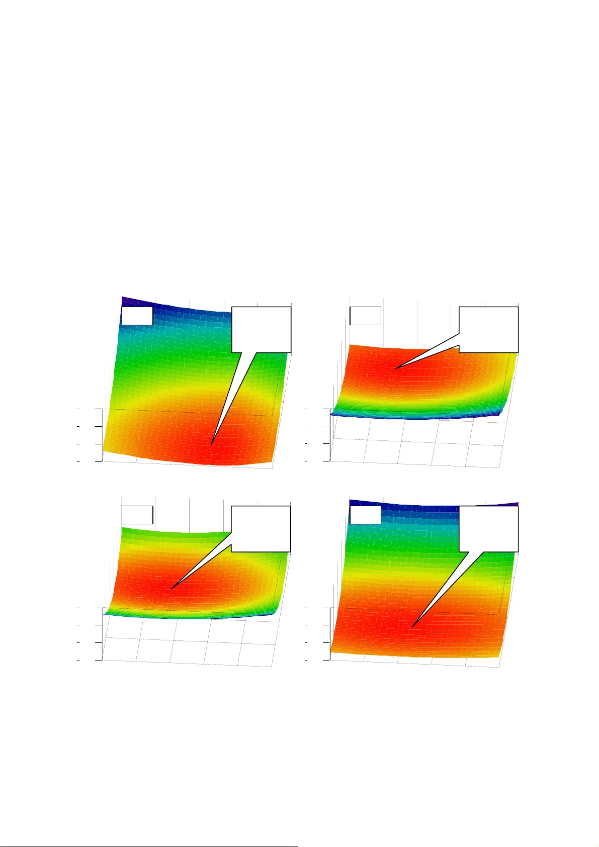
Distribution Fitting 1. Parameters Estima tion under Assumption of A greement between Observation and Model Lorentz JÄNTSCHI Technical University of Cluj -Napoca, 400641 Cluj, Romania; http://lori.a cademicdirect.org Abstract. The methods for parameter estim ation under assumption of agreement between observation and model are reviewed. Th e distribution parameters are obtained for one set of experimental data by using different estimation m ethods under assumption of Gauss-Laplace theoretical di stribution. The results are presented and discussed. Keywords : parameters estim ation; moments; maximum likelihood; minimization of experimental error; Ga uss-Laplace distribution INTRODUCTION Let be Y = (Y 1 , …, Y n ) and X = (X 1 , …, X n ) series of pair observations and the objective be finding of a function f(x; a 1 , …, a m ) for which Ŷ = f(X) is the best possible solution of the approximation Ŷ ~ Y . Reaching this objective suppose finding of the expression of the f function and of the values of a 1 , …, a m parameters. Under assumption of agreement between observation and model the expression of the function f is supposed to be known (or at least supposed, when a search from a given set of a lternative expressions is conducted). Thus, it is remaining to obtain the values of a 1 , …, a m parameters. In order to have a unique solution for the values of the a 1 , …, a m parameters at least m ≤ n is required to be assured. A s er i e s o f alternatives are available for Y ~ f(X) approximation, that ones cons idered most important being revised and exemplified in this r esearch. MATERIALS AND METHODS 1. Minimizing the error of agreem ent (m inimizing the disagreem ent) . Under this assumption a series of alternatives are available (E q(1), different p and q ). When the series Y represents (not null) frequencie s of the distinct observations X then f(x) should be a positiv e function too, and the modulus in numerator of (2 ) and it is no longer required. Assumption of Gauss distribution (Gauss, 1809) of the values of the term s under summation in Eq(1)-(3) are translated into p = 2 , and assump tion of Laplace distribut ion (Laplace, 1812) are translated into p = 1 (Fisher, 1920). The probabili ty density function (PDF) of some representatives of the family containing standard (µ=0, σ =1) Gauss and Laplace distributions are exemplified in Figure 1. Minimizing the error of agreement for different p values give different solutions for the parameters, and as can be seen in Figure 1, are associated with different error shapes. Two particular cases are commonly used to estimate the unknown parameters of a distribution when p = 2 (Fisher and Mackenzie, 1923; Fisher, 1924) . The most general approach to obtain the distribution parameters is to gu ess the valu es or to apply an iterative procedure which reduces in every step the quantity given by the Eq(1) until the reduced qua ntity is much less than the reminded one. . min ) X ( f | ) X ( f Y | ) q , p ( S n 1 i i q p i i = − = ∑ = , q = 0, 1, p / 2 , p ( 1 ) 739 . 2 2 15 ) 5 . 0 ; 0 ( GL ≅ = 707 . 0 2 1 ) 0 . 1 ; 0 ( GL ≅ = 399 . 0 2 1 ) 0 . 2 ; 0 ( GL ≅ π = 342 . 0 ... ) 0 . 3 ; 0 ( GL ≅ = () 321 . 0 2 4 3 ) 0 . 4 ; 0 ( GL 2 3 4 1 2 ≅ π ⋅ ⋅ Γ = − () () () () ⎟ ⎟ ⎟ ⎟ ⎟ ⎠ ⎞ ⎜ ⎜ ⎜ ⎜ ⎜ ⎝ ⎛ ⎟ ⎟ ⎠ ⎞ ⎜ ⎜ ⎝ ⎛ Γ Γ − Γ Γ = 2 p p 2 3 2 1 p 3 p 1 x exp p 1 p 3 2 p ) p ; x ( GL Figure 1. Family of distributions having Gauss and Laplace as representatives 2. Using moments . Under assumption that Y ~ f(X) should be even more accurate (second assumption being the randomness of the error with a zero mean) the approximations is used Σ X i k Y i ~ Σ X i k ·f(X i ) for k ≥ 0. The moments method give m a ximum weight to the first moments, thus a solution a 1 , …, a m of Y ~ f(X) may come from Eq(2) (the m ost convenient way for the general case is the iteration of the a 1 , …, a m parameters staring from som e guess values): ∑ ∑ = = n 1 i i k i n 1 i i k i ) X ( f X ~ Y X , k = 0, 1, … (2) 3. Using central moments . The Y ~ f(X) assumption strongest the approximations Σ X i Y i ~ Σ X i ·f(X i ) and Σ (Y i - Y) k ~ Σ (X i - X) k ·f(X i ) for k ≥ 2. The moments method give maximum weight to first central moments, thus a solution a 1 , …, a m of Y ~ f(X) may c ome from Eq(3). ∑ ∑ = = n 1 i i i n 1 i i i ) X ( f X ~ Y X and ∑ ∑ = = − − n 1 i i k i n 1 i k i ) X ( f ) X X ( ~ ) Y Y ( , k = 2, 3 … (3) 4. Using population statistics . A slight m odification of the previous method may benefit from the availability of population mean, standard de viation, skewness and kurtosis expressions depending on distribution para meters for a large number of well known distributions. For example the µ (mean) and σ (standard deviation) estimated parameters for a normal distributed population come from Eq(4). ∑ ∑ = = = µ n 1 i i n 1 i i i Y Y X and () ⎟ ⎠ ⎞ ⎜ ⎝ ⎛ − ⎟ ⎠ ⎞ ⎜ ⎝ ⎛ µ − = σ ∑ ∑ = = 1 Y Y X n 1 i i n 1 i 2 i i 2 (4) Thus, by using this simple reasoning, if th e theoretical distribution has m parameters ( a 1 , …, a m ), then to obtain a solution for it is necessary to kn ow the expression of the first m central moments and then to solve the equati ons like (4) relating popula tion statistics with their estimators from sample. 5. Maximum likelihood estimation . The principle of the maximum likelihood is that a reasonable estimate for a parameter is the one which maxim izes the probability (P in Eq(5)) GL(x;4) GL(x;3) -2 -1 0 1 2 1 0.5 GL(x;2) GL(x;1) GL(x; 1 / 2 ) of obtaining the experiment al data (Fisher, 1912), a nd the most probable set of a 1 , …, a m parameters will make P a m aximu m (and then MLE is maximum). ∑ = = = n 1 i i 2 2 )) X ( f ( log ) P ( log MLE ( 5 ) Application . One set of experim ental data were taken from literature in order to illustrate the procedures described above (Jän tschi and others, 2009). The measurements were for octanol water partition coefficient (K ow ) for 205 out of 206 polyc hlorinated biphenils expressed in logarithmic scale (log 10 (K ow ), [K ow ]=1). Maximum likelihood estimation was applied for estimation of log(K ow ) of investigated PCB’s. Th e Grubbs test was applied in order to identify the outliers (). One experimental data was considered to be an outlie r and was not included in estimation of distribution. Table 1 contains the experim ental data in ascending order. Table 1. Two data sets of measuremen ts under assumption of normal distribution log(K ow ) for 206 polychlorinated biphenils (sorted data) 4.151; 4.401; 4.421; 4.601; 4.94 1; 5.021; 5.023; 5. 15; 5.18; 5.295; 5. 301; 5.311; 5.3 11; 5.335; 5.343; 5. 404; 5.421; 5.447; 5.452; 5.452; 5.48 1; 5.504; 5.517; 5. 537; 5.537; 5.551; 5.561; 5.572; 5.577; 5.577; 5.62 7; 5.637; 5.637; 5.667; 5.667; 5.671; 5.67 7; 5.677; 5.691; 5. 717; 5.743; 5.751; 5.757; 5.761; 5.767; 5.767; 5.78 7; 5.811; 5.817; 5.827; 5.867; 5.897; 5.89 7; 5.904; 5.943; 5. 957; 5.957; 5.987; 6.041; 6.047; 6.047; 6.047; 6.05 7; 6.077; 6.091; 6.111; 6.117; 6.117; 6.13 7; 6.137; 6.137; 6. 137; 6.137; 6.142; 6.167; 6.177; 6.177; 6.177; 6.20 4; 6.207; 6.221; 6.227; 6.227; 6.231; 6.23 7; 6.257; 6.267; 6. 267; 6.267; 6.291; 6.304; 6.327; 6.357; 6.357; 6.36 7; 6.367; 6.371; 6.427; 6.457; 6.467; 6.48 7; 6.497; 6.511; 6. 517; 6.517; 6.523; 6.532; 6.547; 6.583; 6.587; 6.58 7; 6.587; 6.607; 6.611; 6.647; 6.647; 6.64 7; 6.647; 6.647; 6. 657; 6.657; 6.671; 6.671; 6.677; 6.677; 6.677; 6.69 7; 6.704; 6.717; 6.717; 6.737; 6.737; 6.73 7; 6.747; 6.767; 6. 767; 6.767; 6.797; 6.827; 6.857; 6.867; 6.897; 6.89 7; 6.937; 6.937; 6.957; 6.961; 6.997; 7.02 7; 7.027; 7.027; 7. 057; 7.071; 7.087; 7.087; 7.117; 7.117; 7.117; 7.12 1; 7.123; 7.147; 7.151; 7.177; 7.177; 7.18 7; 7.187; 7.207; 7. 207; 7.207; 7.211; 7.247; 7.247; 7.277; 7.277; 7.27 7; 7.281; 7.304; 7.307; 7.307; 7.321; 7.33 7; 7.367; 7.391; 7. 427; 7.441; 7.467; 7.516; 7.527; 7.527; 7.557; 7.56 7; 7.592; 7.627; 7.627; 7.657; 7.657; 7.71 7; 7.747; 7.751; 7. 933; 8.007; 8.164; 8.423; 8.683; 9.143; 9.603 The experimental data were subject of th e analysis of the agreement between observation and model by using the following methods: minimizing the error of agreement, and maximum likelihood estimation. RESULTS AND DISCUSSION The Gauss-Laplace distribution ge neral form (from Figure 1) and the kurtos is depending on p are given in Figure 2 (Skewness being null). () () () () ⎟ ⎟ ⎟ ⎟ ⎟ ⎠ ⎞ ⎜ ⎜ ⎜ ⎜ ⎜ ⎝ ⎛ ⎟ ⎟ ⎠ ⎞ ⎜ ⎜ ⎝ ⎛ Γ Γ σ µ − − Γ Γ σ = σ µ 2 p p 2 3 2 1 p 3 p 1 x exp p 1 p 3 2 p ) p , , ; x ( GL (6) Figure 2. Gauss-Laplace distribution and its kurtosis () () () p 3 p 1 p 5 ) p ( Ku 2 GL Γ Γ Γ = Ku GL (0)= ∞ Ku GL ( ∞ )=1.8 1 2 3 4 5 6 1 2 3 4 5 6 The Table 2 contains the estimations of the mean ( µ ) and standard deviation ( σ ) parameters for the data sets given in Table 1. The Eq(1) was used when the minimization of the error of agreement was applied. The Eq(5) was used when the maximum likelihood estimation was applied. The values presented in Table 2 were obtained for different p values (0.5-6). The 3D representation of mean, standard deviation and coefficient of variation when minimization of the error of agreem ent is invest igated are graphically represented in Figure 3. The results obtained by maxi mum likelihood estim ation where graphically represented in Figure 4. Table 2. Mean and standard deviation estimators obtained with Eq( 1) and Eq(5) Eq. p µ σ Residues Eq. p µ σ Residues Minimization the error of agreement Minimization the error of agreement Eq(1) q=0 0.5 6.638 1.454 128.595 Eq(1) q= p / 2 2.0 6.380 0.832 384.000 Eq(1) q=0 1.0 6.646 0.822 128.197 Eq(1) q= p / 2 2.5 6.364 0.840 661.000 Eq(1) q=0 1.5 6.580 0.814 143.966 Eq(1) q= p / 2 3.0 6.356 0.862 1250.000 Eq(1) q=0 2.0 6.544 0.748 176.138 Eq(1) q= p / 2 3.5 6.384 0.891 2570.000 Eq(1) q=0 2.5 6.512 0.722 231.718 Eq(1) q= p / 2 4.0 6.400 0.916 5643.000 Eq(1) q=0 3.0 6.512 0.698 323.083 Eq(1) q= p / 2 6.0 6.440 1.000 2·10 5 Eq(1) q=0 3.5 6.512 0.684 472.428 Eq(1) q=p 6.0 6.400 1.046 4·10 7 Eq(1) q=0 4.0 6.512 0.676 720.191 Eq(1) q=p 4.0 6.350 0.960 2·10 5 Eq(1) q=0 6.0 6.472 0.644 5204.000 Eq(1) q=p 3.5 6.314 0.946 5·10 4 Eq(1) q=1 6.0 6.446 0.906 1751 0.000 Eq(1) q=p 3.0 6.298 0.930 16230.000 Eq(1) q=1 4.0 6.430 0.85 6 1646.000 Eq(1) q=p 2.5 6.312 0.936 5431.000 Eq(1) q=1 3.5 6.422 0.84 0 1025.000 Eq(1) q=p 2.0 6.328 0.952 1924.000 Eq(1) q=1 3.0 6.398 0.81 6 678.400 Eq(1) q=p 1.5 6.352 0.984 747.800 Eq(1) q=1 2.5 6.388 0.81 4 485.600 Eq(1) q=p 1.0 6.386 1.102 344.739 Eq(1) q=1 2.0 6.380 0.83 0 383.890 Eq(1) q=p 0.5 6.588 1.924 205.386 Eq(1) q=1 1.5 6.388 0.896 340.000 Eq(1) q=1 1.0 6.388 1.104 344.700 Maximum likelihood estimation Eq(1) q=1 0.5 6.366 2.11 2 427.100 Eq(5) 4 6.476 0.886 -373.810 Eq(1) q= p / 2 0.5 6.650 1.904 156.800 Eq(5) 3 6.468 0.829 -360.790 Eq(1) q= p / 2 1.0 6.486 0.970 185.800 Eq(5) 2 6.464 0.802 -354.208 Eq(1) q= p / 2 1.5 6.412 0.856 249.000 Eq(5) 1 6.510 0.914 -371.620 0 1 2 3 4 1 2 3 4 6. 3 6. 4 6. 5 6. 6 6. 7 0 1 2 3 4 1 2 3 4 0. 7 0. 9 1. 1 1. 3 1. 5 1. 7 1. 9 2. 1 0 1 2 3 4 1 2 3 4 0% 5% 10% 15% 20% 25% 30% Mean Standard error Coefficient of variation Figure 3. Minimizing the error of agreemen t: variation of statistics for different p and q values (p - from Gauss-Laplace distribution and Eq(1), q - from Eq(1)) The analysis of the results obtained by using the minimization agreem ent errors approach (see Table 2 and Figure 3) leads to the following remarks:  The evolution of µ for 0.5 ≤ p ≤ 3 is similar for q=p/2 and q=p as expected.  The evolution of σ for p is similar for q=1, p=p/2 and q=p.  The minimum amplitude for a given p value is obtained for q=1 when the µ is analyzed and for q=0 when the σ is analyzed.  The same trend in variation of µ is observed for p=0.5, p=1, p=1.5, p=2 (up-down- up-down). The highest variation was betwee n q=1 and q=p/2 for p=0.5. The mean values decrease as q increase for a given value of p ≥ 2.5.  The highest values of σ were observed for p=0.5 with a pick for q=1. The same behaviour but with smaller differences were observed for p=1, p=1.5, p=2. A similar behaviour of σ variation was observed for p ≥ 2.5; the smaller variation is observed for p=2.5 (the smaller difference of standard deviation as the q value increased). Figure 4. Likelihood estimation and its maxim um (MLE) for different p values (µ - mean, σ - standard deviation, p - from Gauss-Laplace distribution) The analysis of the results obtained by using the maximum likelihood estimation approach (see Table 2 and Figure 4) leads to the following remarks:  The µ and σ varied slightly with increases of p value (an amplitude of 0.046 was obtained for µ and of 0.112 for σ ); 377.07 375.25 373.44 371.62 361.77 359.25 356.73 354.21 388.02 383.29 378.55 373.81 367.47 365.25 363.02 360.79 p = 1 p = 2 p = 3 p = 4 µ = 6.510 σ = 0.914 MLE=-372 µ = 6.464 σ = 0.802 MLE=-354 µ = 6.468 σ = 0.829 MLE=-361 µ = 6.476 σ = 0.886 MLE=-374  The maximum value of µ and σ were obtained for p=1;  The minimum value of µ and σ were obtained for p=2;  A decrease of µ and σ is observed for p=2. Starting with p=2 their values increase slightly with increases of p values. It may be concluded that as p increases the minimizing of the error of the agreement give more weight to the outliers (see Figure 5). Figure 5. Mean (µ), standard deviation ( σ ) and maximum likelihood (MLE) on a relative scale (between min and max) for p = 1, 2, 3, 4 (Gauss-Laplace distribution) The obtained MLE estimation is presented in Figure 6. Th e associat ed equation and its statistical characteristics are presented in Eq(9). - 375 - 370 - 365 - 360 - 355 - 350 00 . 5 11 . 5 2 Figure 6. Maximum likelihood estimation for distribution of log(K ow ) with 205 of 206 PCBs 207 . 354 MLE ; 008 . 2 p ; 99999 . 0 r 372 ) p ( log 1 . 32 )) p ( (log 6 . 11 )) p ( (log 67 . 3 )) p ( (log 585 . MLE max max 2 2 2 2 3 2 4 2 − = = > − ⋅ + ⋅ − ⋅ − ⋅ = (9) 0 20 40 60 80 100 1 234 µ σ MLE p % max min Eq(9) shows that with a great accuracy the maximum likelihood (MLE=log(P), Eq(5)) of the Gauss-Laplace distribution (GL(x,µ, σ ,p), Eq(6)) can be approx im ated by a fourth order polynomial formula on log(p). For normal (or Gauss) distributed data (as the in vestigated dataset, the common case of the biochemical data) the maximum of this po lynom ial is expected to be near p = 2 and for error function (or Laplace) distributed data (the comm on case of astrophysical data) the maximum of this polynomial is expected to be near p = 1. From this point of view, the observed data shows a very good agreemen t with the normal distribution, m aximum likelihood of the Gauss-Laplace distribut ion being estim ated at p = 2.008. CONCLUSIONS Five methods of parameter estimation under assum ption of agreement between observation and model were reviewed. The abilitie s of minimizing the error of agreement and maximum likelihood estimation were applied on a set of PCBs experimental data. The results showed that as p increases the minim izing of the error of the agreement give more weight to the outliers. As maxim um likelihood estimation is concerned, a powerful model in term s of estimation was obtained when p = 2.008. Acknowledgments. The research was partly supported by UEFISCSU Romania through ID1051/202/2007 grant, PN2 (2007- 2010) national research framework. REFERENCES Fisher, R. A. (1912). On an Absolute Criterion for Fitting Frequency Curves. Messenger of Mathematics 41:155-160. Gauss, C. F. (1809). Theoria Motus Corp orum Coelestium. Perthes et Besser, Hamburg. Translated, 1857, as Theory of Mo tion of the Heavenly Bodies Moving about the Sun in Conic Sections, trans. C. H. Davis. Little, Brown; Boston. Reprinted, 1963, Dover, New York. Laplace, P. S. (1812). Théorie Analyti que des Probabilités. Courcier, Paris. Fisher, R. A. (1920). A Mathematical Exam in ation of the Methods of Determining the Accuracy of an Observation by the Mean Erro r, and by the Mean Square Error. Monthly Notices of the Royal Astr onomical Society 80:758-770. Fisher, R. A. and W. A. Mackenzie. ( 1923). Studies in Crop Variation. II. The manurial response of different po tato varieties. Jour nal of Agricultural Science 13:311-320. Fisher, R. A. (1924). The Conditions Under Which χ 2 Measures the Discrepancy Between Observation and Hypothesis. Journal of the Royal Statisti cal Society 87:442-450. Bolboac ă , S. D., L. Jäntschi, A. F. Sestra ş , R. E. Sestra ş and C. D. Pamfil. (2009). Pearson-Fisher Chi-Square Statistic Revis ited. Manuscrip t submitted for publication and available upon request, 15 pages. Grubbs, F. (1969). Procedures for Detectin g Outlying Observations in Samples. Technometrics 11(1):1-21. Duchowicz, P. R., A. Talevi, L. E. Bruno- Blanch, E. A. Castro. (2008). New QSPR study for the prediction of aqueous solubility of drug-like compounds. Bioorganic & Medicinal Chemistry 16:7944-7955. Jäntschi L., S. D. Bolboac ă , R. E. Sestra ş . (20 09). Meta-Heuristics on Quantitative Structure-Activity Relations hips: A Case Study on Polych lorinated Biphenyls. DOI: 10.1007/s00894-009-0540-z (Online first).