Statistical Physics of Hard Optimization Problems

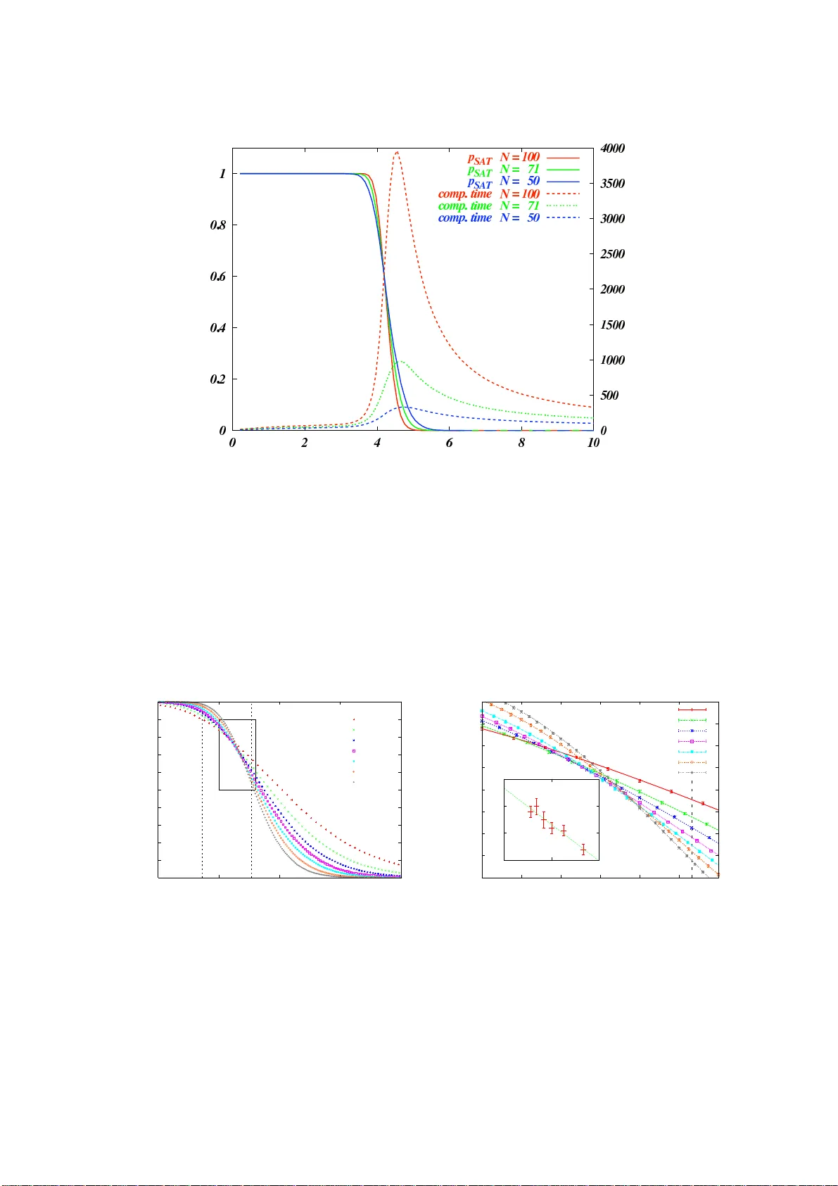
Univ ersit ´ e P aris-Sud 11 F acult ´ e des sciences d’Orsa y Univ erzita Karlo v a v Praze Matematic k o-fyzik ´ aln ´ ı fakulta Thesis presen ted to obtain the degree of Do ctor of Sciences of the Universit y Pa ris XI Do ctor of the Charles Univ ersit y in Prague Sp ecialization: Theoretical Phy sics b y Lenk a ZDEBOR O V ´ A Statistical Ph ysics of Hard Optimization Problems Defended on June 20, 2008, in fron t of the Thesis Committee: Silvi o FRANZ V´ aclav JANI ˇ S thesis adv isor ( Pragu e) Ji ˇ r ´ ı LANGER Stephan MER TE NS referee Marc MEZARD thesis adv isor ( P ari s) Riccardo ZECCH INA referee 2 Ac kno wledgmen t First of all I would lik e to express m y thanks to m y a dvisor Marc M ´ ezard from whom I learned a lot . He sho w ed me how to com bine en thus iasm, patience, computations, and in tuition in the correct prop ortio n to enjo y the delicious taste of the pro cess o f disco v ery . I thank a s well to my advisor V´ acla v Jani ˇ s who guided m y scien tiﬁc steps mainly in the earlier stages of m y work. This w ork would nev er b e possible without the contact and discussions with my col- leagues and colla b orators a ll o ve r the w orld. Without them I w ould feel lost in the v ast w orld of unkno wn. I am grateful to all the organizers o f w orkshops, conferences a nd sum- mer sc ho ols where I had part icipated. I also t hank for invitations on visits and seminars whic h w ere alw ay s ve ry inspiring. I am v ery thankful to the whole Lab oratoire de Ph ysique Th ´ eorique et Mo d ` eles Statis- tiques for a v ery w arm r eception and to all its mem bers for helping me whenev er I needed. I also o w e a lot to m y prof essors from the Charles Unive rsity in Prague, and to m y col- leagues from the Institute of Ph ysics of the Academ y o f Sciences in Prag ue. I also tha nk the referees of m y thesis and other mem b ers of the thesis committee for their interest in m y w ork and for accepting this t ask. I v a lue profoundly the sc holarship g ran ted b y the F renc h Gov ernmen t whic h cov ered the la rgest part of my sta y in F rance. F urther, I appreciated greatly the subv e ntion from the F renc h ministry for higher education and researc h ” cotutelles in ternationales de th´ ese”. I also a c kno wledge gratefully the suppo r t from the FP6 Europ ean net w ork EVER GR OW. My deep est thanks go to my parents fo r their constan t supp ort, encouragemen t, a nd lo v e. Finally , thank y ou Flo fo r a ll the it ems ab ov e and many more. Y ou taught me w ell, and y es I am the Jedi no w. Lenk a Zdeb orov ´ a P aris, Ma y 12, 2008 i ii M´ ym r o diˇ c ˚ um Josefovi a Bo ˇ zenˇ e iii iv Con ten ts Ac kno wledgmen t i Abstract ix F or ew ord xv 1 Hard optimization problems 1 1.1 Imp ortance of optimization problems . . . . . . . . . . . . . . . . . . . . 1 1.2 Constrain t Satisfaction Problems: Setting . . . . . . . . . . . . . . . . . 2 1.2.1 Deﬁnition, factor graph represen tation . . . . . . . . . . . . . . . 2 1.2.2 List of CSPs discussed in this thesis . . . . . . . . . . . . . . . . . 2 1.2.3 Random f a ctor gra phs: deﬁnition and prop erties . . . . . . . . . . 4 1.3 Computational complexit y . . . . . . . . . . . . . . . . . . . . . . . . . . 6 1.3.1 The worst case complexit y . . . . . . . . . . . . . . . . . . . . . . 6 1.3.2 The av erage case hardness . . . . . . . . . . . . . . . . . . . . . . 7 1.4 Statistical ph ysics comes to the scene . . . . . . . . . . . . . . . . . . . . 9 1.4.1 Glance on spin gla sses . . . . . . . . . . . . . . . . . . . . . . . . 9 1.4.2 First encounte r . . . . . . . . . . . . . . . . . . . . . . . . . . . . 10 1.5 The replica symm etric solution . . . . . . . . . . . . . . . . . . . . . . . 11 1.5.1 Statistical ph ysics description . . . . . . . . . . . . . . . . . . . . 11 1.5.2 The replica symmetric solution o n a single graph . . . . . . . . . 12 1.5.3 Av erage o v er the graph ensem ble . . . . . . . . . . . . . . . . . . 14 1.5.4 Application for counting matc hings . . . . . . . . . . . . . . . . . 14 1.6 Clustering and Survey pr o pagation . . . . . . . . . . . . . . . . . . . . . 16 1.7 Energetic 1RSB solution . . . . . . . . . . . . . . . . . . . . . . . . . . . 18 1.7.1 W arning Propag a tion . . . . . . . . . . . . . . . . . . . . . . . . . 18 1.7.2 Surv ey Propagation . . . . . . . . . . . . . . . . . . . . . . . . . . 20 1.7.3 Application to the exact cov er (p ositive 1- in-3 SA T) . . . . . . . . 22 1.8 Lo ose ends . . . . . . . . . . . . . . . . . . . . . . . . . . . . . . . . . . . 23 1.9 Summary of my contributions to the ﬁeld . . . . . . . . . . . . . . . . . . 24 2 Clustering 27 2.1 Deﬁnition of clustering and the 1RSB approach . . . . . . . . . . . . . . 27 2.1.1 Prop erties and equations on trees . . . . . . . . . . . . . . . . . . 29 2.1.2 Bac k to the sparse random graphs . . . . . . . . . . . . . . . . . . 35 2.1.3 Comp endium of t he 1 R SB ca vit y equations . . . . . . . . . . . . . 37 2.2 Geometrical deﬁnitions of clusters . . . . . . . . . . . . . . . . . . . . . . 38 2.3 Ph ysical prop erties of the clustered phase . . . . . . . . . . . . . . . . . . 41 2.4 Is the clustered phase algor it hmically hard? . . . . . . . . . . . . . . . . 41 v vi CONTENTS 3 Condensation 45 3.1 Condensation in a toy mo del of random sub cub es . . . . . . . . . . . . . 45 3.2 New in CSPs, w ell know n in spin glasses . . . . . . . . . . . . . . . . . . 47 3.3 Relativ e sizes of clusters in the condensed phase . . . . . . . . . . . . . . 48 3.4 Condensed phase in ra ndom CSPs . . . . . . . . . . . . . . . . . . . . . . 50 3.5 Is the condensed phase algorithmically hard? . . . . . . . . . . . . . . . . 51 4 F r eezing 53 4.1 F rozen v a r iables . . . . . . . . . . . . . . . . . . . . . . . . . . . . . . . . 53 4.1.1 Whitening: A wa y to tell if solutio ns are frozen . . . . . . . . . . 54 4.1.2 F reezing o n ﬁnite size instances . . . . . . . . . . . . . . . . . . . 54 4.1.3 F reezing tr ansition in 3 -SA T - exhaustiv e en umeratio n . . . . . . 55 4.2 Ca vit y approach to frozen v ariables . . . . . . . . . . . . . . . . . . . . . 57 4.2.1 F rozen v a riables in the en tropic 1RSB equations . . . . . . . . . . 57 4.2.2 The phase tra nsitions: Rig idity and F reezing . . . . . . . . . . . . 60 4.3 P oin t lik e clusters: The lo c k ed problems . . . . . . . . . . . . . . . . . . 62 4.3.1 Deﬁnition . . . . . . . . . . . . . . . . . . . . . . . . . . . . . . . 63 4.3.2 The replica symmetric solution . . . . . . . . . . . . . . . . . . . 63 4.3.3 Small noise reconstruction . . . . . . . . . . . . . . . . . . . . . . 65 4.3.4 Clustering transition in the lo c k ed problems . . . . . . . . . . . . 67 4.4 F reezing - The reason for hardness? . . . . . . . . . . . . . . . . . . . . . 68 4.4.1 Alw a ys a trivial whitening core . . . . . . . . . . . . . . . . . . . 69 4.4.2 Incremen tal algorithms . . . . . . . . . . . . . . . . . . . . . . . . 69 4.4.3 F reezing tr ansition and the p erformance o f SP in 3-SA T . . . . . 71 4.4.4 Lo c k ed problems – New extremely c ha llenging CSPs . . . . . . . . 71 5 Coloring random graphs 75 5.1 Setting . . . . . . . . . . . . . . . . . . . . . . . . . . . . . . . . . . . . . 75 5.2 Phase diag ram . . . . . . . . . . . . . . . . . . . . . . . . . . . . . . . . 76 5.3 Large q limit . . . . . . . . . . . . . . . . . . . . . . . . . . . . . . . . . . 80 5.3.1 The 2 q log q regime: colorabilit y and condensation . . . . . . . . . 81 5.3.2 The q log q regime: clustering a nd rigidit y . . . . . . . . . . . . . 81 5.4 Finite temp erature . . . . . . . . . . . . . . . . . . . . . . . . . . . . . . 82 Conclusions and p ersp ectiv es 85 Key results . . . . . . . . . . . . . . . . . . . . . . . . . . . . . . . . . . . . . 85 Some op en problems . . . . . . . . . . . . . . . . . . . . . . . . . . . . . . . . 85 P ersp ectiv es . . . . . . . . . . . . . . . . . . . . . . . . . . . . . . . . . . . . . 86 App endices 91 A 1RSB ca vit y equations at m = 1 91 B Exact en trop y for the balanced LOPs 95 B.1 The 1 st momen t for o ccupation mo dels . . . . . . . . . . . . . . . . . . . 95 B.2 The 2 nd momen t for o ccupation mo dels . . . . . . . . . . . . . . . . . . . 97 B.3 The results . . . . . . . . . . . . . . . . . . . . . . . . . . . . . . . . . . 98 CONTENTS vii C Stabilit y of the RS solution 101 C.1 Sev eral equiv alent metho ds for RS stability . . . . . . . . . . . . . . . . . 1 01 C.2 Stability of the w a rning propagat io n . . . . . . . . . . . . . . . . . . . . 104 D 1RSB stability 105 D.1 Stability of the energetic 1RSB solution . . . . . . . . . . . . . . . . . . . 106 D.2 1RSB stabilit y at general m and T . . . . . . . . . . . . . . . . . . . . . 108 E P opulations dynamics 111 E.1 P opulation dynamics for b elief propagation . . . . . . . . . . . . . . . . . 11 1 E.2 P opulation dynamics to solv e 1RSB at m = 1 . . . . . . . . . . . . . . . 112 E.3 P opulation dynamics with rew eigh ting . . . . . . . . . . . . . . . . . . . 113 E.4 P opulation dynamics with hard and soft ﬁelds . . . . . . . . . . . . . . . 115 E.5 The p opulation of p opulations . . . . . . . . . . . . . . . . . . . . . . . . 115 E.6 Ho w man y p opulations needed? . . . . . . . . . . . . . . . . . . . . . . . 116 F Algorithms 119 F.1 Decimation based solv ers . . . . . . . . . . . . . . . . . . . . . . . . . . . 119 F.1.1 Unit Clause propaga t io n . . . . . . . . . . . . . . . . . . . . . . . 119 F.1.2 Belief propagatio n based decimation . . . . . . . . . . . . . . . . 120 F.1.3 Surv ey propaga tion based decimation . . . . . . . . . . . . . . . . 124 F.2 Search of impro v emen t based solv ers . . . . . . . . . . . . . . . . . . . . 125 F.2.1 Sim ulated a nnealing . . . . . . . . . . . . . . . . . . . . . . . . . 12 5 F.2.2 Sto c hastic lo cal searc h . . . . . . . . . . . . . . . . . . . . . . . . 125 F.2.3 Belief propagatio n reinforcemen t . . . . . . . . . . . . . . . . . . 127 Reprin ts of Publications 131 [ZDEB-1] LZ, M. M ´ ezard, ” The num b er o f matchings in random graphs”, J. Stat. Me ch. (2006) P05003 . . . . . . . . . . . . . . . . . . . . . . . . 131 [ZDEB-2] E. Manev a, T. Meltzer, J. Raym ond, A. Sp o r t iello, LZ, ”A Hik e in the Phases of the 1-in-3 Satisﬁabilit y ,” Lecture notes of the Les Houc hes Summer School 200 6, Session LXXXV, Complex Systems , V olume 85, 491- 4 98, Elsevier 2007 . . . . . . . . . . . 133 [ZDEB-3] J. Ra ymond, A. Sp ortiello, LZ, ”The Phase Diagram of 1- in-3 Sa t- isﬁabilit y ,” Phys. R ev. E 76 ( 2 007) 011101 . . . . . . . . . . . . . . . . . 135 [ZDEB-4] F. Krzak ala, A. Montanari, F. Ricci-T ersenghi, G . Semerjian, LZ, ”Gibbs Sta tes and the Set of Solutions of Ra ndom Constraint Satisfaction Problems,” Pr o c. Natl. A c ad. Sci. 104 (2007) 10318 . . . . . . . . . . . 1 37 [ZDEB-5] LZ, F. Krzak ala, ”Phase transition in the Color ing of Random Graphs,” Ph ys. R ev. E 76 (20 07) 0311 3 1 . . . . . . . . . . . . . . . . . . 1 39 [ZDEB-6] F. Krzak ala, LZ, ”P otts Glass on Random Gra phs,” Eur. Phys. L ett. 81 (20 08) 5 7005 . . . . . . . . . . . . . . . . . . . . . . 141 [ZDEB-7] F. Krzak a la , LZ, ”Phase T ransitions and Computational Diﬃculty in Random Constraint Sa t isfaction Problems,” J. Phys.: Conf. Ser. 95 (2008) 012012 . . . . . . . . . . . . . . . . . . . 143 [ZDEB-8] T. Mora, LZ, ”Random subcub es as a toy mo del for constrain t satisfaction problems,” J. Stat. Phys. 131 n.6 (2008) 1121 . . . . . . . . 145 [ZDEB-9] LZ, M. M ´ ezard, ” Hard constraint satisfa ction pro blems,” preprin t arXiv:0803.2955v1 . . . . . . . . . . . . . . . . . . . . . . . . . . 14 7 viii CONTENTS [ZDEB-10] J. Ardelius, LZ, ”Exhaustiv e en umeration un v eils clustering and freezing in ra ndo m 3- SA T,” preprin t a rXiv:0804.0362v1. . . . . . . . . . . 1 4 9 Bibliograph y 153 Index 165 ABSTRA CT ix Title : Stat istical Ph ysics of Hard Optimization Problems Author : L enk a Z deb oro v´ a Abstract : Optimization is fundamen tal in many ar eas of science, fro m computer science and information theory to enginee ring a nd statistical phy sics, as w ell a s to biology or so cial sciences . It t ypically in v olv es a large n um b er of v ariables and a cost function dep ending on these v aria bles. Optimization problems in the NP-complete class are particularly diﬃcult, it is b eliev ed that the num b er of op era t io ns required to minimize the cost function is in the most diﬃcult cases exp onen tial in the system size. Ho w ev er, ev en in an NP-complete problem the practically arising instances migh t , in f a ct, be easy to solve. The principal question w e address in this thesis is: Ho w to recognize if an NP-complete constraint satisfaction problem is ty pically hard a nd what are the main reasons for this? W e adopt approac hes from the statistical ph ysics of disordered systems, in part icular the cav ity metho d dev elop ed originally to describ e g lassy systems. W e describ e new prop erties of the space of solutions in tw o o f the most studied constraint satisfaction pro blems - r a ndom satisﬁabilit y and random graph coloring. W e suggest a relation b et w een the existence of the so-called frozen v a riables and the algorithmic hardness of a problem. Based on these insigh ts, w e in tro duce a new class o f problems whic h w e na med ”lo c k ed” constraint satisfaction, where the statistical description is easily solv able, but from the algorithmic p oin t of view they ar e ev en more c hallenging than the canonical satisﬁabilit y . Keyw ords : Constraint satisfaction problems, combinatorial optimization, ra ndo m color- ing problem, av erage computational complexit y , ca vit y metho d, spin glasses, replica sym- metry breaking, Bethe appro ximation, clustering of solutions, phase transitions, message passing, b elief propagation, satisﬁabilit y threshold, reconstruction on trees. x ABSTRA CT RESUME xi Titre : Ph ysique statistique des probl ` emes d’optimisation Autheur : Lenk a Z deb oro v´ a R´ esum ´ e : L’optimisation est un concept fondamen tal dans b eaucoup de domaines scien- tiﬁques comme l’informatique, la th´ eorie de l’informatio n, les sciences de l’ing ´ enieur et la phys ique statistique, ainsi que p our la biologie et les sciences so ciales. Un probl` eme d’optimisation met typiq uemen t en jeu un nombre imp or t a n t de v ariables et une fonc- tion de co ˆ ut qui d ´ epend de ces v a r ia bles. La classe des probl` emes NP-complets est particuli ` eremen t diﬃcile, et il est comm un ´ emen t admis que, dans le pire des cas, un nom- bre d’op ´ erations expo nentiel dans la taille du probl ` eme est n ´ ecessaire p our minimiser la fonction de co ˆ ut. Cep endan t, m ˆ eme ces probl` emes p euv eut ˆ etre faciles ` a r´ esoudre en pratique. La principale question consid ´ er ´ ee dans cette th ` ese est commen t reconna ˆ ıtre si un probl ` eme de satisfaction de contrain tes NP-complet est ”t ypiquemen t” diﬃcile et quelles son t les raisons p our cela ? Nous suiv ons une appro c he inspir ´ ee par la ph ysique statistique des syst ` emes desordonn ´ es, en particulier la m ´ etho de de la cavit ´ e d ´ ev elopp ´ ee originalemen t p our les syst ` emes vitreux. Nous d ´ ecriv o ns les propri ´ et ´ es de l’espace des solutions dans deux des probl` emes de satisfaction les plus ´ etudi ´ es : la satisﬁabilit ´ e et le coloriage al´ eatoire. Nous sugg ´ erons une relatio n en tre l’existence de v a r ia bles dites ”gel ´ ees” et la diﬃcult´ e alg o rithmique d’un probl ` eme donn ´ e. Nous introduisons aussi une nouv elle class e de pro bl` emes, que nous app elons ”probl` emes v errouill´ es”, qui pr ´ esen tent l’a v antage d’ˆ etre ` a la fois facilemen t r ´ esoluble a nalytiquemen t, du p oint de vue du com- p ortemen t moy en, mais ´ egalemen t extrˆ ememen t diﬃciles du p oint de vue de la rec herc he de solutio ns dans un cas donn ´ e. Les mots clefs : Probl ` emes d’optimisation de contrain tes, optimisation com binatoire, probl ` emes de colo r ia ge, complexit ´ e de calcul moy enne, m´ etho de de la ca vit ´ e, v erres de spins, brisure de la sym ´ etrie des r´ epliques, approx imation de Bethe, regroup emen t des so- lutions en amas, transitions de phases, passage de messages , pro pa gation des convictions, seuil de satisﬁabilit´ e, reconstruction sur des arbres. xii RESUME ˇ CESK ´ Y ABSTRAKT xiii N´ azev : St a tistic k´ a fyzik a tˇ e ˇ zk´ yc h optimaliza ˇ cn ´ ıc h ´ uloh Autor : Lenk a Zdeb orov´ a Abstrakt : Optimalizace je fundamen t´ aln ´ ı k oncept v mnoha vˇ edn ´ ıc h ob orec h, p oˇ c ´ ına je p o ˇ c ´ ıtaˇ cov ou v ˇ edou a teori ´ ı informace, p ˇ res in ˇ zen´ yrstv ´ ı a statistick ou f yziku, aˇ z p o bi- ologii ˇ ci ek onomii. Optimaliza ˇ cn ´ ı ´ uloha se t ypic ky skl´ ad´ a z minimalizace funk ce z´ avisej ´ ıc ´ ı na ve lk ´ em mno ˇ zstv ´ ı promˇ enn´ ych. Probl´ em y z takzv an´ e NP- ´ upln ´ e t ˇ r ´ ıdy jsou obzvl´ a ˇ st ˇ e slo ˇ zit ´ e, v ˇ e ˇ r ´ ı se, ˇ ze p oˇ cet o p erac ´ ı p o t ˇ rebn´ y k nalezen ´ ı ˇ re ˇ sen ´ ı v tom nejtˇ e ˇ z ˇ s ´ ım p ˇ r ´ ıpadˇ e ro ste exp o nenci´ alnˇ e s p o ˇ ctem prom ˇ en´ yc h. Nicm ´ en ˇ e i pr o NP- ´ upln ´ e ´ uloh y pla t ´ ı, ˇ ze praktic k ´ e p ˇ r ´ ıpady mohou b´ yt jedno duc h ´ e. Hla vn ´ ı ot´ azk a, kterou se zab´ yv´ a tato pr´ ace, je: Jak rozp oznat, zda je NP- ´ upln ´ y probl´ em splnitelnosti p o dm ´ ınek v typic k ´ em p ˇ r ´ ıpadˇ e t ˇ e ˇ zk´ y a ˇ c ´ ım je t a to sloˇ zitost zp ˚ usob ena? K t´ eto ot´ azce p ˇ ristupujeme s vyu ˇ zit ´ ım znalost ´ ı ze stati- stic k´ e fyziky neusp o ˇ r´ adan´ yc h, a zejm´ ena sk eln ´ yc h, syst ´ em ˚ u. P op ´ ı ˇ seme no v ´ e vlastnosti prostoru ˇ re ˇ sen ´ ı v e dv ou z nejv ´ ıce studov an ´ yc h optimalizaˇ cn ´ ıc h probl ´ em ˚ u – splnitelnosti n´ a ho dn´ yc h Bo oleov sk´ yc h formul ´ ı a barve n ´ ı n´ a ho dn´ yc h g r a f ˚ u. Navrhne me existenci vz- tah u mezi t ypic k ou algoritmic k ou slo ˇ zitost ´ ı a existenc ´ ı takzv anˇ e zamrzl´ yc h pro mˇ enn´ yc h. Na z´ aklad ˇ e tˇ ec h to p o znatk ˚ u zk onstruujeme nov ou t ˇ r ´ ıdu pro bl ´ em ˚ u, kter ´ e jsme na zv a li ”uzamkn ut ´ e”, zde je statistic k´ y p opis mno ˇ zin y v ˇ sec h ˇ re ˇ sen ´ ı p omˇ ern ˇ e jedno duch´ y, ale z a lgoritmic k ´ eho p ohledu jsou tyto ty pic k ´ e p ˇ r ´ ıpady tˇ ec hto probl´ em ˚ u je ˇ st ˇ e te ˇ z ˇ si ne ˇ z v k anonic k ´ em probl´ em u splitelnosti Bo oleo vsk´ yc h form ul ´ ı. Kl ´ ıˇ cov ´ a slo v a : Probl ´ em y splnitelnosti p o dm ´ ınek, kom binatorick ´ a optimalizace, barv en ´ ı n´ a ho dn´ yc h graf ˚ u, pr ˚ umˇ ern´ a algoritmick ´ a sloˇ zitost, meto da k avit y , spinov ´ a skla, na r u ˇ sen ´ ı symetrie r eplik, Betheho apro ximace, shluk o v´ an ´ ı ˇ re ˇ sen ´ ı, f´ azov ´ e p ˇ rechody , p os ´ ıl´ an ´ ı zpr´ av, propagace domn ˇ enek, pr´ ah splnitelnosti, rek onstrukc e na stromec h. xiv ˇ CESK ´ Y ABSTRAKT F orew ord P .-G. de Gennes in his foreword t o the b o ok ”Stealing t he gold – A celebration of the pioneering ph ysics of Sam Edw ards” wrote: But he { me aning S. Ed w ar ds } also has another p assion, which I { me aning P. - G. de Genne s } c al l ”The se ar ch f o r unic orns.” T o chase unic orns is a delic ate e nterprise. Me dieval Britons pr a ctise d it w i th gr e a t enthusiasm (and this stil l holds up to now: r e ad Harry Potter). Sir Samuel Edwar ds is not far fr om the gal lant knights of the twel f th c entury. Disc overing a str an g e animal, appr o aching it without fe ar, then not ne c essaril y harnessing the cr e atur e, but r a p id ly dr aw ing a plausible sketch of its main fe atur es. One b e autiful unic orn pr ancing in the magic gar den of Physics has b e en names ”Spin glass.” It i s r ar e : not m any pur e br e e ds of Spin glasse s hav e b e en found in Natur e. B ut we have al l watche d the unpr e dictable jumps of this b e ast. A nd we have love d its story – initiate d by Edwar ds and A nderson. Unicorn is a m ythical animal, describ ed in the b o ok o f Job, together with another strange and fascinating creature whic h is less p eaceful: the leviathan. Leviathans are described a s immense terrible monsters, invincible b easts. Most p eople prefer not to ev en think a b out them. This thesis tells a story ab out what happens when the ﬁerce and mys terious b eaut y of a unicorn meets with the in vincibilit y of a leviathan. xv xvi F OREW ORD Chapter 1 Hard optimization problem s In this o p ening chapter we intr o duc e the c onstr aint satisfaction pr oblems an d dis c uss brieﬂy the c omputer sc i enc e appr o ach to the c omputational c omplexity. We r eview the studies of the r andom satisﬁability pr o b lem in the c o n text of aver age c omputational c om- plexity in v e stigations. We des c ri b e the c onne ction b e twe en spi n glasses and r andom CSPs and highligh t the most in ter esting r es ults c oming o ut fr om this analo gy. We explain the r eplic a symmetric appr o ach to these pr oblems and show its usefulness on the example of c ounting of m a tchings [Z DEB-1]. Then we r eview the survey pr op agation appr o ach to c onstr ain t satisfaction on an example of 1-i n - K satisﬁability [ZDEB-3]. Final ly we sum- marize the ma in c ontributions o f the author to the adv a nc es in the statistic al ph ysics of har d o ptimization pr oblems, that ar e elab or ate d in the r est of the thesis. 1.1 Imp ort ance of optimizatio n p roblems Optimization is a common concept in man y areas of human activities. It t ypically inv olve s a large n um b er of v ariables, e.g. particles , agen ts, cells or no des, and a cost function dep ending on these v ariables, suc h as energy , measure of risk or exp enses. The problem consists in ﬁnding a state of v ariables whic h minimizes the v alue of t he cost function. In this thesis w e will concen tr ate on a subset of optimization problems the so-called c onstr ain t satisfaction pr oblems (CSPs). Constraint satisfaction problems a r e one of the main building blo c ks o f complex systems studied in computer science, informatio n theory and statistical phys ics. Their wide range of applicability arises from their very general nature: given a set of N discrete v ariables sub ject to M constrain ts, the CSP consists in deciding whether there exists an assignmen t of v ariables whic h satisﬁes sim ultaneously all the constraints . And if such an assignmen t exists then w e aim at ﬁnding it. In computer science, CSPs are at the core of computational complexit y studies: the satisﬁabilit y of b o olean formulas is the canonical example of a n in trinsically hard, NP- complete, problem. In information theory , error correcting co des also rely on CSPs. The transmitted informatio n is encoded in to a co dew ord satisfying a set of constrain ts, so t hat the information ma y b e retriev ed after transmission through a noisy c hannel, using the kno wledge of the constrain t s satisﬁed by the co dew o r d. Man y other practical problems in sc heduling a collection of tasks, in electronic design engineering or artiﬁcial inte lligence are view ed as CSPs. In statistical ph ysics the interest in CSPs stems from their close relation with the theory of spin glasses. Answ ering if frustration is av oidable in a system is the ﬁrst, and sometimes highly non trivial, step in understanding the lo w temp erature b eha viour. 1 2 CHAPTER 1 . HARD OPTIMIZA TION PR OBLEMS A k ey p o int is to understand how diﬃcult it is t o solv e practical instances of a con- strain t satisfaction problem. Ev eryda y experience conﬁrms tha t sometimes it is v ery hard to ﬁnd a solutio n. Man y CSPs require a com bination o f heuristics and com bina- torial searc h metho ds to b e solv ed in a reasonable time. A key question w e address in this t hesis is thus why and whe n are some instances of these problems in trinsically hard. Answ ering this question has, next to its theoretical in terest, sev eral practical motiv ations • Understanding where the ha r dness comes from helps to push the p erformance of CSPs solv ers to its limit. • Understanding whic h instances are ha r d helps to av oid them if the nature of the giv en practical problem p ermits. • Finding the very hard problem might b e in teresting for cryptographic application. A piv otal step in this direction is the understanding of the onset of hardness in random constrain t satisfaction problems. In practice random constrain t satisfaction problems are either regarded as extremely hard as there is no obvious structure to b e explored or as extremely simple as they p ermit probabilistic description. F urthermore, random constrain t satisfaction mo dels are spin glasses a nd w e shall th us b orrow metho ds from the statistical phys ics of disordered systems. 1.2 Constr aint Satisfaction Problems: Setting 1.2.1 Deﬁnition, factor graph represen tation Constrain t Satisfaction Problem (CSP): Consider N v aria bles s 1 . . . , s N taking v alues from the domain { 0 , . . . , q − 1 } , and a set of M constrain ts. A constrain t a concerns a set of k a diﬀeren t v a riables whic h w e call ∂ a . Constrain t a is a function fro m all p ossible assignmen ts of t he v ariables ∂ a to { 0 , 1 } . If the constraint ev aluates to 1 w e sa y it is satisﬁed, and if it ev aluates to 0 w e say it is violated. The constraint satisfaction problem consists in de ciding whether there exists an assignmen t of v aria bles wh ich satisﬁes sim ult a neously all the constrain ts. W e call suc h a n assignmen t a solution of the CSP . In ph ysics, the v aria bles represen t q - state P otts spins (or Ising spins if q = 2). The con- strain ts represen t ve ry general (non- symmetric) in teractions b etw een k a -tuples of spins. In Bo o lean constraint satisfaction problems ( q = 2) a liter al is a v aria ble or its negation. A clause is then a disjunction (logical O R) of literals. A handy represen tation for a CSP is the so-called fa c tor g r aph , see [KFL01] for a review. F a ctor graph is a bipartite graph G ( V , F , E ) where V is the set of v a riables (v ariables no des, represen ted b y circles) a nd F is the set of constraints (function nodes, represen ted b y squares). An edge ( ia ) ∈ E is presen t if the constrain t a ∈ F inv olv es the v ariable i ∈ V . A constrain t a is connected to k a v ariables, their set is denoted ∂ a . A v ariable i is connected to l i constrain ts, their set is denoted ∂ i . F or clarity w e sp ecify the factor g raph represen tation fo r the graph coloring and exact cov er problem in ﬁg. 1.1, b oth deﬁned in the following section 1.2.2. 1.2.2 List of CSPs discu ssed in this thesis Here w e deﬁne constrain t satisfaction problems whic h will b e discuss ed in the follow ing. Most o f them are discussed in the classical reference b o ok [GJ79]. The most studied 1.2. CONSTRAINT SA TISF A CTION PROBLEMS: SETTING 3 000 000 000 111 111 111 000 000 000 000 111 111 111 111 00 00 00 11 11 11 Figure 1.1: Example of a fa ctor graph r epresen tation for the coloring (left) and the exact co v er (right) problems. The function no des (squares) in the graph coloring are satisﬁed if and only if their t w o neighbours (circles) are in diﬀerent states (tak e diﬀeren t colors). The function no des (squares ) in the exact co ve r pro blem are satisﬁed if exactly one v ar ia ble (circle) around t hem takes v alues 1 (full) and the others 0 (empty ). constrain t satisfaction problems are deﬁned o v er Bo olean v ariables, q = 2, s i ∈ { 0 , 1 } . Sometimes w e use equiv alently t he notation with Ising spins s i ∈ {− 1 , +1 } . CSPs with Bo olean v ariables that w e shall discuss in this thesis are: • Satisﬁabilit y ( SA T) problem : Constraints are clauses, that is logical disjunc- tions of literals (i.e., v aria bles or their negations). Example o f a satisﬁable for mula with 3 v ariables and 4 clauses (constrain ts) and 10 literals: ( x 1 ∨ x 2 ∨ ¬ x 3 ) ∧ ( x 2 ∨ x 3 ) ∧ ( ¬ x 1 ∨ ¬ x 3 ) ∧ ( x 1 ∨ ¬ x 2 ∨ x 3 ). • K -SA T : Satisﬁabilit y problem where ev ery clause in v olv es K literals, k a = K for all a = 1 , . . . , M . • Not-All-Equal SA T : Constrain ts are satisﬁed eve rytime except when all the lit- erals they in v olv e are TR UE or all o f them a re F ALSE. • Bicoloring : Constrain ts are satisﬁed except when a ll v aria bles they inv olv e ar e equal. Bicolor ing is Not - All-Equal SA T without negations. • X OR-SA T : Constrain ts ar e logical XORs of literals. • Odd (resp. Ev en) Parit y Checks : A constrain t is satisﬁed if the sum of v ariables it inv olv es is o dd (resp. ev en). Odd parity chec ks are XORs without negations. • 1-in- K SA T : Constraints are satisﬁed if exactly one of the K literals they in v olve is TRUE. • Exact Cov er, or p osit iv e 1-in- K SA T : Constrain ts are satisﬁed if exactly one of the K v a riables they inv olv e is 1 (o ccupied). E xact co v er, or p ositiv e 1- in- K SA T, is 1-in- K SA T without negations. • P erfect matc hing : Nodes of the or ig inal gr a ph b ecome constrain ts, v ar iables are on edges and determine if the edge is or is not in the matc hing, see ﬁg. 1.5. 4 CHAPTER 1 . HARD OPTIMIZA TION PR OBLEMS Constrain ts are satisﬁed if exactly one of the K v ariables they in v olv e is 1 (b elongs to the matching). Note that p erfect matc hing is just a v a r ian t of the Exact Cov er • Occupation problems are deﬁned b y a binary ( K + 1) comp o nen t v ector A . All constrain ts inv olv e K v aria bles, and a re satisﬁed if the sum of v a riables they in v olve r = P ∂ a s i is such that A r = 1. • Lo c k ed Occupation Problems (LOPs) : If the v ector A is suc h that A i A i +1 = 0 for all i = 0 , . . . , K − 1, and all the v aria bles are presen t in at least t w o constrain ts. W e will also consider in a great detail one CSP with q - ary v ar ia bles: The graph coloring with q colors: Ev ery constrain t inv olv es tw o v ariables and is satisﬁed if the t w o v ariables are not assigned the same v a lue (colo r). In phys ics the q -ary v ariables are called P otts spins. 1.2.3 Random factor graphs: deﬁnition and prop erties Giv en a constrain t satisfaction problem with N v ariables and M constraints, the c on- str aint density is deﬁned as α = M / N . Denote b y R ( k ) the probability distribution of the degree of constrain ts (num b er of neighbours in the factor gra ph), and b y Q ( l ) the probabilit y distribution of the degree of v ar iables. The av erage connectivit y (degree) of constrain ts is K = k = ∞ X k =0 k R ( k ) . (1.1) The a v erage connectivit y of v ariables is c = l = ∞ X l =0 l Q ( l ) . (1.2) The constrain t densit y is t hen asymptotically α = M N = l k = c K . (1.3) A random f a ctor gra ph with a giv en N and M is then created as follows: Draw a sequence { l 1 , . . . , l N } of N n um b ers from the distribution Q ( l ). Subseq uen tly , draw a sequence { k 1 , . . . , k M } of M n um b ers from the distribution R ( k ), suc h that P M a =1 k i = P N i =1 l i . The r andom factor gr aph is draw n uniformly at random from all the factor graphs with N v aria bles, M constrain ts and degree sequences { l 1 , . . . , l N } and { k 1 , . . . , k M } . Another deﬁnition leading to a Poiss onian degree distribution is used of ten if the degree of constraints is ﬁxed to K and the num b er of v ariables is ﬁxed to N . There are  N K  p ossible p ositions for a constrain t. Eac h of these p ositions is tak en with proba bility p = cN K  N K  . (1.4) The num b er of constraints is then a P oissonian random v aria ble with a v erage M = cN /K . The degree of v ariables is distributed according to a Poissonian law with av erage c Q ( l ) = e − c c l l ! . (1.5) 1.2. CONSTRAINT SA TISF A CTION PROBLEMS: SETTING 5 If K = 2 these are the random Erd˝ os-R ´ en yi gra phs [ER59 ]. This deﬁnition w orks also if constrain ts are c hanged for v aria bles, that is if the degree of v ariables and the n um b er of constrain ts are ﬁxed, as in e.g. the matchin g problem. The random factor gra phs are called r e gular if b oth the degrees of constrain ts and v ariables are ﬁxed, R ( k ) = δ ( k − K ) and Q ( l ) = δ ( l − L ). In section 4 .3 w e will also use the trunc a te d Poissonian degree distribution l ≤ 1 : Q ( l ) = 0 , (1.6a) l ≥ 2 : Q ( l ) = 1 e c − ( c + 1) c l l ! . (1.6b) The a v erage connectivit y for the truncated P oissonian distribution is then l = c e c − 1 e c − ( c + 1) . (1.7) In the ca vit y approach, the so-called ex c ess de gr e e distribution is a crucial quan tity . It is deﬁned as follows : Cho ose an edge ( ij ) a t random and consider the probability distribution of t he n um b er of neigh b o ur s of i except j . The v ariables (a na logously for constrain ts) excess degree distribution th us reads q ( l ) = ( l + 1) Q ( l + 1) l , r ( k ) = ( k + 1 ) R ( k + 1) k . (1.8) W e will alwa ys deal with factor g raphs where K and c are of order one, and N → ∞ , M → ∞ . These are called sp arse r a n dom fa ctor gr a phs . Concerning the phys ical prop erties of sparse ra ndom factor graphs the t w o deﬁnitions of a random graph with P oissonian degree distribution are equiv alen t. Some prop erties (e.g. the annealed av er- ages) can how ev er depend on the details of the deﬁnition. The tree-like prop erty of sparse random factor graphs — Consider a random v ariable i in the factor graph. W e wan t to estimate the av erage length of the shortest cycle going through v ariable i . Consider a diﬀusion alg orithm spreading in to all direction but the one it came from. The probability that this diﬀusion will arrive bac k to i in d steps reads 1 −  1 − 1 N  P d j =1 ( γ l γ k ) j , (1.9) where γ l = l 2 /l − 1 and γ k = k 2 /k − 1 are the mean v alues of the excess degree distribution (1.8). The proba bilit y (1.9) is almost surely zero if d ≪ log N log γ l γ k . (1.10) An imp ortan t prop erty follows : As long as the degree distributions R ( k ) and Q ( l ) hav e a ﬁnite v ariance the sparse random f a ctor graphs are lo cally tr ees up to a distance scaling as log N (1.10). W e deﬁne this as the tr e e-like prop ert y . In this thesis w e conside r only degree distributions with a ﬁnite v a r ia nce. A general- ization to other cases (e.g. the scale-free net w orks with long- tail degree distributions) is not straigh tforward and man y of the results whic h are a symptotically exact on the tree- lik e structures w ould b e in general only approximativ e. W e o bserv ed, see e.g. ﬁg . 2.2, 6 CHAPTER 1 . HARD OPTIMIZA TION PR OBLEMS that many of the nontriv ial pro p erties predicted asymptotically on the tree-like graphs seems to b e reasonably precise ev en on graphs with ab out N = 10 2 − 10 4 v ariables. It means that the asymptotic b eha viour sets in rather early and do es not, in fact, require log N ≫ 1. 1.3 Computation al complexit y 1.3.1 The w orst case complexit y Theoretical computer scien tists dev elop ed the computat io nal complexit y theory in order to quan tify ho w har d problems can b e in the worst p ossible case. The most imp o rtan t and discusse d complexit y classe s ar e the P , NP and NP-complete. A problem is in the P (p olynom ial) cl a ss if there is an algorithm whic h is able to solv e the problem for an y input instance o f length N in at most cN k steps, where k and c a r e constants indep enden t of the input instance. The formal deﬁnitions of what is a ”problem”, its ”input instance” a nd an ”algorithm” w a s formalized in the theory of T uring machines [Pap94], where the deﬁnition w ould b e: The complexit y class P is the set of decision problems that can b e solve d by a deterministic T uring mac hine in p olynomial time. A simple example of p olynomial problem is sorting a list o f N real n um b ers. A problem is in the NP class if its instance can b e stored in memory of p olyno- mial size and if the correctness of a prop osed result can b e c hec k ed in p olynomial time. F ormally , the complexit y class NP is the set of decision problems that can b e solv ed b y a non-deterministic T uring mac hine in p olynomial time [P a p94], NP stands fo r non- deterministic po lynomial. Whereas the deterministic T uring mac hine is basically an y of our to da y computers, the non- deterministic T uring mac hine can p erform unlimited num - b er of parallel computations. Th us, if for ﬁnite N there is a ﬁnite n um b er of p ossible solutions all of them can b e c hec k ed sim ultaneously . This class con tains many problems that we w ould lik e to b e a ble to solv e eﬃcien tly , including the Bo olean satisﬁabilit y prob- lem, t he tra v eling salesman problem or the g r aph coloring. Problems whic h do not b elong to the NP class a re for example coun ting t he n um b er of solutions in Bo olean satisﬁability , or the random energy mo del [Der80, D er81]. All the p o lynomial problems are in the NP class. It is not know n if all the NP problems are p o lynomial, and it is considered by man y to b e the most c hallenging problem in theoretical computer science. It is also one o f the sev en, and one of the six still o p en, Millennium Prize Problems that w ere stated b y the Cla y Mathematics Institute in 20 00 (a correct solution to eac h o f these problems results in a $1,00 0,000 prize for the author). A ma jority of computer scien tists, how ev er, b eliev es that the negativ e answ er is the correct one [Gas02]. The concept o f NP-complete problems was in tro duced b y Co ok in 197 1 [Co o71]. All the NP problems can b e p olynomially reduced to any NP-complete problem, t hus if an y NP-complete problem would b e p olynomial then P=NP . Co ok prov ed [Co o7 1] tha t the Bo o lean satisﬁabilit y problem is NP-complete. Karp so o n after added 2 1 new NP- complete problems to the list [Kar72]. Since then thousands of other problems hav e b een sho wn to be NP-complete b y reductions from other problems previously sho wn to b e NP-complete; man y of these are collected in the Ga r ey a nd Johnson’s ”Guide to NP-Completeness ” [GJ79]. Sc haefer in 19 78 prov ed a dic hotomy theorem for Bo olean ( q = 2) constraint satis- faction pro blems. He sho w ed that if the constrain t satisfaction problem has one of the 1.3. COMPUT A TIONAL COMPLEXITY 7 follo wing four pro p erties then it is p olynomial, otherwise it is NP-complete. (1) All con- strain ts are suc h that s i = 1 fo r all i is a solution or s i = 0 fo r all i is a solution. (2) All constrain ts concern at most tw o v ariables (e.g. in 2-SA T). (3) All constrain ts are linear equations mo dulo tw o (e.g. in XOR-SA T). (4) All constrain ts are the so-called Horn clauses or all of them are the so-called dual Horn clauses. A Horn clause is a disjunction of v aria bles suc h tha t at most one v ariable is not negated. A dual Horn clause is when a t most one v ar iable is negated. A similar dic hotomy theorem exists for 3- state v ariables, q = 3, [Bul02 ]. Generalization for q > 3 is not kno wn. 1.3.2 The a v erage c ase hardn ess Giv en the presen t kno wledge, it is often said that all the p olynomial problems are easy and all the NP-complete problems are v ery hard. But, indep enden tly if P=NP or not , ev en p olynomial pr o blems migh t b e practically v ery diﬃcult, a nd some (o r ev en most) instances of the NP-complete problems migh t b e practically ve ry easy . An example of a still diﬃcult p olynomial problem is the primality testing, a ﬁrst p olynomial algorithm was disco vered b y [AKS04]. But a ”pro o f ” of remaining diﬃcult y is the EFF prize [EFF] of $100,00 0 to the ﬁrst individual or group who disco vers the ﬁrst prime num b er with at least 10,000 ,0 00 decimal digits. And how hard are the NP-complete problems? One w ay to answe r is tha t under restrictions on the structure an NP-complete problem might b ecome p o lynomial. May b e the most famous example is 4-coloring of maps (planar factor graphs) whic h is p o lynomial. Moreo v er, it w as a long standing conjecture t ha t ev ery map is colo r a ble with 4 colors, pro v en b y App el and Hake n [AH77b, AH77a]. In terestingly enough 3- coloring of maps is NP-complete [GJ79]. But there are a lso settings under whic h the pro blem stays NP-complete and y et almost ev ery instance can b e solv ed in p olynomial time. A historically imp ortan t example is the Bo olean satisﬁability where eac h clause is g enerated b y selecting literals with some ﬁxed probabilit y . Goldb erg introduced this rando m ensem ble and sho w ed that the av erage running time of the Da vis-Putnam algorithm [DP60, DLL62] is p olynomial for almost all c hoices of parameter settings [G ol79, GPB82]. Th us in the eighties some computer scien tist tended to think that all the NP-complete problems are in fact on a v erage easy and it is hard to ﬁnd the evil instances whic h make s them NP-complete. The breakthrough came at the b eginning of the nineties when Cheeseman, Kanefsky and T a ylor aske d ”Where the r e al l y hard pro blems are?” in their pap er of the same name [CKT91]. Shortly after Mitche ll, Selman and Lev esque came up with a similar w ork [MSL92]. Both groups simply to o k a diﬀeren t random ensem ble of the satisﬁability (in the second case) and coloring (in the ﬁrst case) instances: the length of clauses is ﬁxed to b e K and they are draw n randomly as describ ed in sec. 1.2.3. They observ ed that when the densit y of clauses α = M / N is small the existence of a solution is very lik ely and if α is large the existence o f a solution is ve ry unlik ely . And the r e al ly har d instances w ere lo cated nearb y the critical v alue o riginally estimated to b e α s ≈ 4 . 25 in the 3-SA T [MSL92]. The hardness w as judged from the median running time of the Davis - Putnam-Logemann-Lov eland (DPLL) bac ktra cking-based algorithm [DP60, DLL 6 2], see ﬁg. 1.2. This whipp ed aw ay the t hough ts that NP-complete pro blems might in fact b e easy on a v erage. Man y other studies and observ ations follow ed. The hard instances of random K -satisﬁabilit y b ecame ve ry fast imp o rtan t b enchm arks for t he b est algo rithms. Moreo v er, there ar e some indications that critically constrained instances might a pp ear 8 CHAPTER 1 . HARD OPTIMIZA TION PR OBLEMS Figure 1.2: The easy-hard-easy patt ern in the random 3-SA T formulas as the constrain t densit y is c hanged. F ull lines are probabilities that a formula is satisﬁable. Dashed lines is the medium running time o f t he DPLL algorithm. This ﬁgure is courtesy of Riccardo Zecc hina. in real-w orld applications. One may imag ine that in a real w orld situatio n the amount of constrain ts is giv en b y the nature of the problem, a nd v aria bles usually corresp ond to something costly , th us the comp etitiv e designs contain the smallest p ossible num b er of v ariables. 0 0.1 0.2 0.3 0.4 0.5 0.6 0.7 0.8 0.9 1 3.5 4 4.5 5 5.5 probability of satisfiability density of constraints a s a d N=25 N=35 N=45 N=55 N=65 N=80 N=100 0.5 0.55 0.6 0.65 0.7 0.75 0.8 0.85 0.9 4 4.05 4.1 4.15 4.2 4.25 4.3 probability of satisfiability density of constraints a s N=25 N=35 N=45 N=55 N=65 N=80 N=100 4 4.1 4.2 4.3 0 0.02 0.04 Figure 1.3: Pro ba bilit y that a random 3- SA T formula is satisﬁable as a function of the constrain t densit y . In the inset on the left ﬁgure is the p osition of the crossing p oin t b et w een curv es corresp onding to diﬀeren t sizes a s a function of 1 / N . It seems to extrap olate to the a na lytical v alue α s = 4 . 267 [MZ02, MMZ06]. This ﬁg ure should b e put in con trast with ﬁg. 4.1 where the same plot is presen ted f or the freezing transition with a mu ch smaller size of the inset. Giv en a rando m K -SA T form ula of N v ariables the probabilit y that it is satisﬁable, plotted in ﬁg. 1.3 for 3-SA T, b ecomes more and more lik e a step-function as the size N gro ws. An analogy with phase transitions in ph ysics cannot b e ov erlo ok ed. The existence 1.4. ST A TISTICAL PHYSICS COMES TO THE SCENE 9 and sharpness of the threshold w ere partially prov ed [F ri99]. The b est kno wn pro babilistic b ounds of the threshold v a lue in 3- SA T are 3 . 520 for the low er b ound [KKL03, HS03] and 4 . 506 for the upp er b o und [DBM00]. Numerical estimates of the asymptotic v a lue of the threshold a re α s ≈ 4 . 17 [KS94], α s ≈ 4 . 258 [CA96], α s ≈ 4 . 27 [MZK + 99b, MZK + 99a]. The ﬁnite size scaling of the curv es in ﬁg. 1.3 is quite inv olv ed as the crossing p oin t is mo ving. That is wh y the early n umerical estimates of the threshold w ere ve ry inaccurate. The work of Wilson [Wil02], moreo v er, show ed that the exp erimental sizes are to o small and the asymptotic regime for the critical exp onen t is not reac hed in an y of the curren t empirical works. The study of XOR-SA T indeed sho ws a crosso v er in the critical exp onen t at sizes whic h are not accessible for K -SA T [LR TZ0 1]. The studies o f random K -SA T op ened up the exciting p ossibilit y to connect the hardness with an algorithm-indep enden t prop ert y , lik e t he satisﬁabilit y phase transition. But what exactly makes the instances near to the threshold hard remained an op en question. 1.4 Statistic al physics c omes to the sc e ne 1.4.1 Glance on spin glasses Spin glass is one o f the most in teresting puzzles in statistical ph ysics. An example of a spin glass material is a piece of gold with a small fraction of iron impurities. Ph ysicist, on contrary to the rest of the h uman p opulation, are in terested in the b ehav iour of these iron impurities a nd not in the piece of gold itself. A new t yp e of a phase transition w a s observ ed from t he high temp erature parama g netic phase to the low temp erature spin glass phase, where the magnetization of eac h impurit y is fr oze n to a non- zero v a lue, but there is no long range ordering. More than 3 0 y ears ago Edw ards and Anderson [EA75 ] in tro duced a lattice mo del for suc h ma g netic disordered alloys H = − X ( ij ) J ij S i S j − h X i S i , (1.11) where S i ∈ {− 1 , +1 } are Ising spins on a 3-dimensional lattice, the sum runs ov er all the nearest neigh b ours, h is the external mag netic ﬁeld and the in teraction J ij is random (usually Gaussian or randomly ± J ). The solutio n of the Edw ards-Anderson mo del stays a lar g ely op en problem ev en to da y . The mean ﬁeld v ersion of the Edw ards-Anderson mo del was in tro duced by Sherrington and Kir kpatric k [SK75], the sum in the Hamiltonian (1.11) then runs ov er all pairs ( ij ) as if the underlying la t tice w ould b e f ully connected. Sherrington and Kirkpatrick called their pap er ”Solv able Mo del of a Spin-Gla ss”. They w ere indeed righ t, but the correct solution came only ﬁv e y ears later b y P arisi [Par80c, P ar80 b, P ar80 a ]. Parisi’s r e plic a symmetry br e aking (RSB) solution of the Sherrington-Kirkpatric k mo del gav e rise to a whole new theory of the spin glass phase and of the ideal glass transition in structural glasses. The exactness of the Parisi’s solution w as, how ev er, in doubt till 2000 when T alagrand provide d its r ig orous pro of [T al06]. The relev ance of the R SB picture for the original Edw ards-Anderson mo del is widely discussed but still unkno wn. A diﬀeren t mean ﬁeld vers ion o f the Edw ards-Anderson mo del w as in tro duced by Viana and Bra y [VB85], the la t tice underlying the Hamiltonia n (1.11) is then a random graph of ﬁxed av erage connectivit y . The complete solution of the Viana- Br ay mo del is also still a n op en pro blem. 10 CHAPTER 1 . HARD OPTIMIZA TION PR OBLEMS 1.4.2 First encounte r The Viana-Bray mo del of spin glasses can also b e view ed a s random gr aph bi-partitioning (or bi- coloring at a ﬁnite temp erature). The p eculiarit y of the spin glass phase will surely ha v e some interes ting conseque nces for the optimization problem itself. Indeed, the close connection b etw een optimization problems and spin glass syste ms brough t forw ard a whole collection of theoretical to ols to analyze the structural prop erties o f the optimiza- tion problems. All started in 1985 when M´ ezard and P arisi realized that the r eplica theory can b e used to solv e t he bipart it e weigh ted ma t c hing problem [MP85]. Let us quote fro m the in tro duction of this w ork: ”This b e i n g a kind o f pione erin g p ap er, we have de cide d to pr esent the metho d { me aning the r eplic a metho d } on a r ather simple pr oblem (a p olyno- mial one) the w eighte d matching. In this pr ob lem one is given 2 N p oi n ts i = 1 , . . . , 2 N , with a matrix of distanc e l ij , and one lo oks for a matching b etwe en the p oints (a set of N links b etwe en two p oints such that at e ach p oint o n e and only one link arrives) of a minimal len gth.” Using the replica symmetric (RS) approach they computed the av erage minimal length, when the elemen ts of t he ma t r ix l ij are random iden tically distributed indep enden t v ariables. Shortly after F u and Anderson [F A86] used the replica metho d to treat the graph bi-partitioning problem. They w ere the ﬁrst to suggest t ha t, p ossibly , the existence of a phase tra nsition in the a v erage b ehav iour will aﬀect the actual implemen tation and p er- formance of lo cal optimization tec hniques, and that this ma y also play an imp ortant role in the complexit y theory . Only later, suc h a b eha viour w as indeed disco v ered empirically b y computer scien tists [CKT91, MSL92]. The replica metho d also serv ed to compute t he a v erage minimal cost in the random tra v eling salesmen problem [MP86a, MP86b]. P artitioning a dense rando m graph into more than tw o groups a nd the coloring problem of dense random graphs we re discuss ed in [KS87]. L a ter some of the early results w ere conﬁrmed rigoro usly , mainly t hose concerning the matchin g pro blem [Ald01, L W04]. All these early solv ed mo dels are formulated on dense or even fully connected gr a ph. T hus the replica metho d a nd where needed the replica symmetry breaking could b e used in its original form. Another example of a ”fully connected” optimization problem whic h w as solv ed with a statistical physic s approac h is the n um b er partitioning problem [Mer98, Mer00]. And what ab out our customary random K - satisﬁability , whic h is deﬁned on a sparse graph? Monasson and Zecc hina w ork ed out the replica symmetric solution in [MZ96, MZ97]. It was immediately o b vious t ha t this solution is not exact as it larg ely ov eres- timates the satisﬁabilit y threshold, the replica symmetry has to b e brok en in random K -SA T. An in teresting observ ation was made in [MZK + 99b]: They deﬁned the backbone of a f orm ula as the set of v ariables whic h take the same v alue in all the ground-state con- ﬁgurations 1 . No extensiv e ba ckbone can exist in the satisﬁable phase in the limit of large N . If it w ould, then adding an inﬁnitesimal fraction of constraints w ould almost surely cause a con tradiction. At the satisﬁability threshold an extensiv e ba c kb one may app ear. The authors of [MZK + 99b] suggested that the problem is computatio nally hard if the bac kb one app ears discon tinuous ly and easy if it app ears con tinuously . They sup- p orted this b y replica symmetric solution of the SA T pro blem with mixed 2-clauses and 1 In CSPs with a discrete symmetry , e.g . graph colo ring, this symmetry has to b e taken into acco unt in the de ﬁnitio n o f the backbone. 1.5. THE REPLICA SYMMETRIC SOLUTION 11 3-clauses, the so-called 2 + p -SA T. Ev en if the replica symmetric solution is not correct in random K - SA T and ev en if it o v erlo oks many o ther imp ortant phenomena the concept of ba ckbone is fruitful and w e will discuss its generalization in chapter 4. Ho w to deal with the replica symmetry breaking on a sparse tree-lik e gr aph w as an op en question since 1985, when Viana and Br ay [VB85] in tro duced their mo del. The solu- tion came only in 2000 when M ´ ezard a nd Parisi published their pap er ”Bethe lattice spin glass revisited” [MP01]. They sho w ed how to treat corr ectly and without appro ximations the ﬁrst step of replica symmetry breaking (1R SB) and describ ed how , in the same w a y , one can in principal deal with more steps of replica symmetry breaking, this extension is ho w ev er n umerically v ery diﬃcult. But b efore explaining the 1RSB metho d we describ e the general replica symmetric solutions. And illustrate its usefulness on the problem of coun ting matc hings in g raphs [ZDEB-1]. Only then w e describe the main results o f the 1RSB solution and illustrate the metho d in the 1-in- K SA T problem [ZDEB-3]. After w e list sev eral ” lo ose ends” whic h app ear ed in this appro ac h. Finally w e summarize the main contribution o f this t hesis. This will b e t he departure p oin t for the follo wing part of t his thesis whic h con tains mo st of the original results. 1.5 The repl ica symmetric solution The replica symmetric (RS) solution on a lo cally tree-lik e graph consists o f tw o steps: (1) Compute the partition sum and all the other quan tities of in terest as if the graph w ould b e a tree. (2) The r eplica symmetric assumption: Assume that the correlations induced by long lo ops decay fa st enough, suc h that this tree solution is also correct on the only lo cally tree-lik e graph. Equiv alent names used in literature for the replica symme tric solution are Bethe-P eierls appro ximation (in part icular in the earlier physic s references) o r b elief pro pa gation (in computer science or when using the iterative equation as an algorithm to estimate the marginal probabilities - magnetizations in ph ysics). Both these conv enien tly abbreviate to BP . 1.5.1 Statistical p h ysics description Let φ a ( ∂ a ) b e the ev aluating function fo r the constrain t a dep ending o n the v a r ia bles neigh b ourho o ding with a in t he factor graph G ( V , F , E ). A satisﬁed constrain t has φ a ( ∂ a ) = 1 and violated constraint φ a ( ∂ a ) = 0. The Hamiltonian can then b e writ- ten as H G ( { s } ) = M X a =1  1 − φ a ( ∂ a )  . (1.12) The energy cost is th us one for ev ery violated constrain t. The corresp onding Boltzmann measure on conﬁguratio ns is: µ G ( { s } , β ) = 1 Z G ( β ) e − β H G ( { s } ) , (1.13) 12 CHAPTER 1 . HARD OPTIMIZA TION PR OBLEMS where β is t he in v erse temp erature and Z G ( β ) is the partition function. The marginals (magnetizations) χ i s i are deﬁned as the probabilities that the v ariable i tak es v alue s i χ i s i = 1 Z G ( β ) X { s j } ,j =1 ,...,i − 1 ,i +1 ,...,N e − β H G ( { s j } ,s i ) . (1.14) The go al is to compute the in t ernal energy E G ( β ) a nd the en tropy S G ( β ). F or β → ∞ (zero temp erature limit) these t w o quantities giv e the gro und state prop erties. W e a r e in terested in the ”thermo dynamic” limit of larg e graphs ( N → ∞ ), and w e shall compute exp ectatio ns o v er ensem bles of graphs of the densities of thermo dynamical p oten tials ǫ ( β ) = E [ E G ( β )] / N and s ( β ) = E [ S G ( β )] / N , as well as the a v erage free energy densit y f ( β ) = − 1 β N E [log Z G ( β )] = 1 N E [ F G ( β )] = ǫ ( β ) − 1 β s ( β ) . (1.15) The r eason for this interes t is that, for reasonable gra ph ensem bles, F G ( β ) is self-a v eraging. This means that the distribution of F G ( β ) / N b ecomes more and more sharply p eak ed around f ( β ) when N increases. 1.5.2 The replica symmetric solution on a single graph j i a j a b Figure 1.4: P arts of the factor graph used to compute ψ a → i s i and χ j → a s j . First supp o se that the underlying factor gra ph is a tree, part of this tree is depicted in ﬁg. 1.4. W e deﬁne messages ψ a → i s i as the probabilit y that no de i tak es v alue s i on a mo diﬁed gra ph where all constrain ts a round i apart a we re deleted, a nd χ j → a s j as the prob- abilit y that v ariable j tak es v alue s j on a mo diﬁed graph obtained b y deleting constraint a . On a tree these messages can b e computed recursiv ely as ψ a → i s i = 1 Z a → i X { s j } ,j ∈ ∂ a − i φ a ( { s j } , s i , β ) Y j ∈ ∂ a − i χ j → a s j ≡ F ψ ( { χ j → a } ) , (1.16a) χ j → a s j = 1 Z j → a Y b ∈ ∂ j − a ψ b → j s j ≡ F χ ( { ψ b → j } ) , (1.16b) where Z a → i and Z j → a are nor malization constants, the factor φ a ( { s } , β ) = 1 if the con- strain t a is satisﬁed by the conﬁguration { s } and φ a ( { s } , β ) = e − β if not. W e denote b y ψ a → i the whole v ector ( ψ a → i 0 , . . . , ψ a → i q − 1 ) and ana logically χ j → a = ( χ k → a 0 , . . . , χ j → a q − 1 ). This is one form o f the b elief pr op aga tion (BP) equations [KFL01, P ea82], sometimes called sum-pro duct equations. The probabilities ψ , χ are interpreted as messages (b eliefs) living on the edges of the factor graph, with the consistency rules (1.16a) and (1.1 6 b) on the 1.5. THE REPLICA SYMMETRIC SOLUTION 13 function and v ar ia ble no des. Equations (1.16) are usually solv ed b y iteratio n, the name message p ass i n g is used in this contex t. In the following it will b e simpler not to consider the ”t w o-lev els” equations (1.16 ) but ψ a → i s i = 1 Z j → i X { s j } ,j ∈ ∂ a − i φ a ( { s j } , s i , β ) Y j ∈ ∂ a − i Y b ∈ ∂ j − a ψ b → j s j ≡ F ( { ψ b → j } ) , (1.17) where Z j → i = Z a → i Q j ∈ ∂ a − i Z j → a . Notice t hat on simple gra phs, i.e., when either l i = 2 for a ll i = 1 , . . . , N or k a = 2 for all a = 1 , . . . , M , the form (1.17) simpliﬁes further. And on constrain t satisfaction pro blems on simple graphs (e.g. the matc hing or colo ring problems) the ”t w o-lev els” equations are almost nev er used. Assuming that one has found the ﬁxed p oint of the b elief propagation equations (1.16a-1.16b), one can deduce the v arious marginal probabilities and the free energy , en trop y etc. The marginal pro babilit y (1.14) of v ariable i estimated b y the BP equations is χ i s i = 1 Z i Y a ∈ ∂ i ψ a → i s i . (1.18) T o compute the f r ee energy w e ﬁrst deﬁne the free energy shift ∆ F a + ∂ a after addition of a function no de a and all the v ariables i a round it, and the free energy shift ∆ F i after addition of a v aria ble i . These are giv en in general b y: e − β ∆ F a + ∂ a = Z a + ∂ a = X { s i } ,i ∈ ∂ a φ a ( { s i } , β ) Y i ∈ ∂ a Y b ∈ ∂ i − a ψ b → i s i , (1.19a) e − β ∆ F i = Z i = X s i Y a ∈ ∂ i ψ a → i s i . (1.19b) The total free energy is then obtained by summ ing ov er all constrain ts and subtracting the terms coun t ed twic e [MP01 , YFW03 ]: F G ( β ) = X a ∆ F a + ∂ a − X i ( l i − 1)∆ F i . (1.20) This form of the free energy is v ariational, i.e., the deriv ativ es ∂ ( β F G ( β )) ∂ χ i → a and ∂ ( β F G ( β )) ∂ ψ a → i v anish if and only if the probabilities χ i → a and ψ a → i satisfy ( 1.16a-1.16b). This allo ws to compute easily the inte rnal energy as E G ( β ) = ∂ β F G ( β ) ∂ β = − X a ∂ β Z a + ∂ a Z a + ∂ a . (1.21) The en trop y is then obtained as S G ( β ) = β [ E G ( β ) − F G ( β )] . (1.22) All the equations (1.16)-(1.2 2) are exact if the graph G is a tree. The replica symmetric approac h consists in assuming that all correlations decay fa st enough that application of eqs. (1.16)-(1.22) on a large tree-lik e graph G giv es asymptotically exact results. These equations can b e used either on a g iven graph G or to compute the av erage o v er the graph ( a nd disorder) ensem ble. 14 CHAPTER 1 . HARD OPTIMIZA TION PR OBLEMS 1.5.3 Av erage o v er the graph ensem ble W e no w study the ty pical instances in an ensem ble of graphs. W e denote the av erage o v er the ensem ble by E ( · ). W e assume that the random factor-gra ph ensem ble is give n b y a pr escrib ed degree distribution Q ( l ) for v ar ia bles and R ( k ) for constrain ts. Let us call P ( ψ ) and O ( χ ) the distributions of messages ψ and χ ov er all the edges of a large ty pical factor graph fro m the ensem ble. They satisfy the follo wing self-consisten t equations P ( ψ ) = ∞ X l =1 q ( l ) Z l Y i =1  d χ i O ( χ i )  δ  ψ − F ψ ( { χ i } )  , (1.23a) O ( χ ) = ∞ X k =1 r ( k ) Z k Y i =1  d ψ i P ( ψ i )  δ  χ − F χ ( { ψ i } )  , (1.23b) where the functions F ψ and F χ represen t the BP equations (1.16a-1.16b), q ( l ) and r ( k ) are the excess degree distributions deﬁned in (1 .8). If there is a disorder in the inte raction terms, as e.g. the negations in K -SA T, we av erage o v er it at the same place as ov er the ﬂuctuating degree. Solving equations (1.23a-1.23b) to obtain the distributions P and O is not straigh t- forw ard. In some cases (on regula r factor gr a phs, at zero temp erature, etc.) it can b e argued that the distributions P , O are sums of Dir a c delta functions. Then the solution of eqs. (1.23a-1.23b) can b e obtained ana lytically . But in general distributional equa- tions of this t yp e are not solv able analytically . Ho wev er, a n umerical tec hnique called p opulation dynamics [MP01] is very eﬃcien t fo r their resolution. In appendix E w e giv e a pseudo-co de desc ribing ho w the p opulation dynamics tec hnique works . Once the distributions P and O are kno wn t he av erage of the free energy densit y can b e computed by av eraging (1.20) o v er P . This a v erage expression for the free energy is again in its v ar ia tional f o rm (see [MP01]) , i.e., the functional deriv ativ e δf ( β ) δ P ( h ) v anishes if and only if P satisﬁes (1.32). The a v erage energy and en trop y densit y are thus expresse d again via the partia l deriv ativ es. F act o r ized solution — As w e men tioned, on the ense mble of random regular factor graphs (without disorder in the interactions) the solution of equations (1.23) is ve ry simple: P ( ψ ) = δ ( ψ − ψ reg ), Q ( χ ) = δ ( χ − χ reg ), where ψ reg and χ reg is a self-consisten t solution of (1.16). This is b ecause in the t hermo dynamical limit an inﬁnite neigh b ourho o d of ev ery v ariable is exactly iden tical th us also the mar ginal probabilities ha v e to b e iden tical in ev ery ph ysical solution. 1.5.4 Application for coun ting matc hings T o demonstrate ho w the replica symmetric metho d w orks to compute the en trop y , that is the logarithm of the num b er of solutions, w e review the r esults for ma t ching on sparse random g raphs [ZDEB-1]. The reasoning wh y the replica symmetric solution is exact fo r the matc hing pro blem is done on the lev el of self-consistency che c ks in [ZDEB-1]. And [BN06] hav e work ed out a rigorous pro of for graphs with b ounded degree and a la rge girth (length of t he smallest lo o p). Consider a graph G ( V , E ) with N v ertices ( N = | V | ) and a set of edges E . A matching (dimerization) of G is a subset of edges M ⊆ E suc h that each v ertex is inciden t with at most one edge in M . In other w o rds the edges in the matc hing M do not to uch eac h 1.5. THE REPLICA SYMMETRIC SOLUTION 15 other. The size of the matching , | M | , is the num b er o f edges in M . Our goal is to compute the en tro p y of matc hings of a given size on a t ypical large Erd˝ o s-R ´ en yi random gra ph. W e describ e a mat c hing by the v a riables s i = s ( ab ) ∈ { 0 , 1 } assigned to eac h edge i = ( ab ) of G , with s i = 1 if i ∈ M and s i = 0 otherwise. The constraints that tw o edges in a matc hing cannot touc h imp ose that, on eac h v ertex a ∈ V : P b, ( ab ) ∈ E s ( ab ) ≤ 1. T o complete our stat istical ph ysics description, w e deﬁne for each giv en g raph G an energy (or cost) function whic h give s, for eac h matc hing M = { s } , t he num b er of unmatc hed v ertices: H G ( M = { s } ) = X a E a ( { s } ) = N − 2 | M | , (1.24) where E a = 1 − P ∂ b s ( ab ) . In the factor graph represen tation w e transform the g raph G in to a fa ctor graph F ( G ) as follo ws (see ﬁg. 1.5): T o eac h edge of G corresp onds a v ar iable no de (circle) in F ( G ); to eac h v ertex o f G cor r esp onds a function no de (square) in F ( G ). W e shall index t he v ariable no des b y indices i, j, k , . . . a nd function no des b y a, b, c, . . . . The v a riable i ta k es v alue s i = 1 if the corr esp onding edge is in the matc hing, and s i = 0 if it is not. The w eigh t of a function no de a is φ a ( { ∂ a } , β ) = I X i ∈ ∂ a s i ≤ 1 ! e − β (1 − P i ∈ ∂ a s i ) , (1.25) where ∂ a is the set o f a ll the v ariable no des whic h are neigh b ours of the function no de a , and the t otal Bo ltzmann weigh t o f a conﬁguration is 1 Z G ( β ) Q a φ a ( { ∂ a } , β ). 0 1 0 1 0 1 00 00 11 11 00 00 11 11 0 1 000 000 000 000 000 000 111 111 111 111 111 111 0000 1111 Figure 1.5: On the left, example of a graph with six no des and six edges. On the r igh t, the corresp onding factor graph with six function no des (squares) and six v ariable no des (circles). The b elief propagation equation (1.16) b ecomes χ i → a s i = 1 Z b → a X { s j } I s i + X j ∈ ∂ b − i s j ≤ 1 ! e − β (1 − s i − P s j ) Y j ∈ ∂ b − i χ j → b s j , (1.26) where Z b → a is a norma lizat io n constant. In statistical ph ysics the more common form of the BP equations uses analog of local mag netic ﬁelds instead o f pr o babilities. F or ev ery edge b et w een a v ariable i and a f unction no de a , w e deﬁne a c avity ﬁeld h i → a as e − β h i → a ≡ χ i → a 0 χ i → a 1 . (1.27) The recursion relatio n b et w een cav ity ﬁelds is then: h i → a = − 1 β log " e − β + X j ∈ ∂ b − i e β h j → b # . (1.28) 16 CHAPTER 1 . HARD OPTIMIZA TION PR OBLEMS The expectation v alue (with resp ect to the Boltzmann distribution) of the o ccupation n um b er s i of a giv en edge i = ( ab ) is equal to h s i i = 1 1 + e − β ( h i → a + h i → b ) . (1.29) The free energy shifts needed to compute the total fr ee energy (1.2 0) are e − β ∆ F a + i ∈ ∂ a = e − β + X i ∈ a e β h i → a , (1.30a) e − β ∆ F i = 1 + e β ( h i → a + h i → b ) . (1.30b) The energy , related to the size o f the match ing via (1.24), is then E G ( β ) = X a 1 1 + P i ∈ ∂ a e β (1+ h i → a ) . (1.31) This is the sum of the pro ba bilities that no de a is not matc hed. The distributional equation (1.23) b ecomes O ( h ) = ∞ X k =1 r ( k ) Z k Y i =1  d h i O ( h i )  δ " h + 1 β log e − β + X i e β h i !# . (1.32) And the av erage f ree energy is explicitly f ( β ) = E [ F G ( β )] N = − 1 β ∞ X k =0 R ( k ) Z k Y i =1  d h i O ( h i )  log e − β + X i e β h i ! + c 2 β Z d h 1 d h 2 O ( h 1 ) O ( h 2 ) log  1 + e β ( h 1 + h 2 )  . (1.33) Where R ( k ) is the connectivit y distribution of the function no des, that is the connec- tivit y distribution of t he o riginal graph, c is the a v erage connectivit y . The distributional equations are solv ed via the p opulation dynamics metho d, see app endix E. Fig. 1.6 then presen ts the resulting av erage entrop y as a function of size of the matc hing. 1.6 Cluste ring and Surv ey pr o pagation As w e said previously in the random K -SA T the replica symmetric solution is not gener- ically correct. M ´ ezard and P arisi [MP01] understo o d ho w to deal prop erly and without appro ximations with the r eplica symmetry breaking on random sparse graphs, that is ho w to take in to a ccount the correlatio ns induced b y long lo ops. More precisely in their approac h only the one-step (at most t w o-step on the r egular gra phs) replica symmetry breaking solution is n umerically feasible. An yho w, suc h a pro gress op ened the do or to a b etter understanding of t he optimization problems on sparse graphs. The K - satisﬁabilit y pla y ed again the prominen t role. T o compute the ground state energy within the 1RSB approac h we can restrict only to energetic considerations as describ ed in [MP03], w e call this approa c h the e n er getic zer o temp er atur e limit . Applying this metho d to K -satisﬁabilit y leads to sev eral outstand- ing results [MPZ02 , MZ02], w e describ e the t hree most remark able ones. So on af t er, analog results w ere obtained f or man y other optimization problems, for example graph coloring [MPWZ02, BMP + 03, KPW04], verte x co v er [Zho03], bicoloring of h yp er-graphs [CNR TZ03], X OR-SA T [F L R TZ01, MR TZ03 ] or latt ice glass mo dels [BM02, RBMM04]. 1.6. CLUSTE RING AND SUR VEY PR OP A GA TION 17 0 0.1 0.2 0.3 0.4 0.5 0.6 0.7 0.8 0 0.05 0.1 0.15 0.2 0.25 0.3 0.35 0.4 0.45 0.5 Entropy Size of matching c=6 c=3 c=2 c=1 s 0 (e 0 ) Figure 1.6: En tropy densit y s ( m ) as a function of relativ e size of the matching m = | M | / N for Erd˝ os-R´ en yi random graphs with mean degrees c = 1 , 2 , 3 , 6 . The lo w er curv e is the ground state en tropy densit y f o r all mean degrees. The curv es are obtained b y solving eqs. (1.32)-(1.33) with a p opulation dynamics, using a p opulation of sizes N = 2 · 10 4 to 2 · 1 0 5 and the num b er of iterations T = 10000. Clustering — It w as known already in the ” pre-1RSB-cav ity era” that replica sym- metry broken solution is needed to solv e r andom K - SA T. Suc h a need is in terpreted as the existenc e of man y metastable w ell-separated states, in the case of highly de- generate ground state this leads to a clustering of solutions in the satisﬁable phase [BMW00, MPZ02, MZ02]. The energetic 1RSB ca vit y metho d deals with clusters con- taining f rozen v ariables (clusters with bac kb ones), that is v ar ia bles whic h ha v e the same v alue in a ll the solutions in the cluster. It predicts how man y o f suc h clusters exist at a given energy , the logarithm of this n umber divided b y the system size N deﬁnes the complexit y function Σ( E ). According to the energetic ca vit y metho d for 3- SA T, clusters exist, Σ(0) 6 = 0, for constrain t densit y α > α SP = 3 . 9 2 [MPZ02, MZ02]. It was conjectured [MPZ02 , MZ02] that there is a link b etw een clustering, ergo dicit y breaking, existence of many metastable states and the diﬃculty of ﬁnding a ground state via lo cal algorithms. The critical v alue α SP w as called the dynamic al transition and the region of α > α SP the har d-SA T phase. Clusters w ere view ed as a kind of pure states, ho w ev er, in the view of man y a go o d formal deﬁnition w as missing. It w as also often referred to some sort of geometrical separation b et w een diﬀerent clusters. A particularly p o pula r one is the following: Clusters are connected comp o nen t s in the graph where solutions are the no des and t w o solutions are adjacen t if t hey diﬀer in only d v ariables. Dep ending on the mo del a nd author the v alue of d is either one of d is a ﬁnite num b er of d is said to b e a n y sub-extensiv e n um b er. The notion of x -satisﬁabilit y , the existence of pairs of solutions at a distance x , leads to a rigorous pro of of existence of exp onen tially man y g eometrically separated clusters [MMZ05, DMMZ08, AR T06]. 18 CHAPTER 1 . HARD OPTIMIZA TION PR OBLEMS The satisﬁabilit y threshold computed — The energetic 1RSB cav ity metho d al- lo ws to compute the ground state energy and th us also the satisﬁabilit y thr eshold α s . In 3-SA T its v alue is α s = 4 . 2 6 67 [MPZ02, MZ02, MMZ06]. This v alue is computed as a solution of a closed distributional equation. This time there is an excellen t a g reemen t with t he empirical estimations. Is the one step of replica symmetry br eaking suﬃcien t to lo cate exactly the satisﬁability threshold? The stabilit y of the 1RSB solution w a s in v estigated in [MPR T04], the 1 RSB energetic cavit y w as sho wn to describe correctly the ground state energy for 4 . 15 < α < 4 . 39 in 3-SA T. In particular, it yields the conjecture that the lo cation of the satisﬁabilit y threshold is actually exact. F rom a rigorous p oin t of view it w as pro ven that the 1RSB equations giv e an upp er b ound on the satisﬁabilit y threshold [FL03, FL T03, PT04]. Surv ey Propagation: a revolutionary algorithm — The most sp ectacular result w as the deve lopmen t of a new message passing algorithm, the surv ey propagat io n [MZ02, BMZ05]. Before the replica and ca vit y analysis w ere used to compute the quenc hed a v erages of thermo dynamical quan tities. Using alw ays the self-a v eraging prop ert y that the av erage of certain (no t all) quantities is equal to their v alue on a large given sample. M ´ ezard and Z ecc hina applied the energetic 1R SB cav ity equations, later called surv ey propagation, on a single large g r aph. This resulted in a n algo r ithm whic h is arguably still the b est kno wn for larg e instances of r andom 3-SA T near to the satisﬁability threshold. And ev en more in t eresting than its p erformance is the conceptual a dv ance this brough t in to applications of statistical ph ysics to optimization problems. 1.7 Energet i c 1RSB solut i on In this section we deriv e the energetic zero- temp erature limit o f the 1RSB metho d. When applied to the satisﬁabilit y problem this leads, b et w een others, to the calculation of the satisﬁabilit y threshold and to the surv ey propagation equations and algorithm. W e illustrate this on the 1- in-3 SA T problem. Before do ing so w e ha v e to in tro duce the w arning propagat ion equations, on whic h the deriv a tion o f the surv ey propag a tion relies. 1.7.1 W arning P r opagation In general warning propagat io n (min-sum) is a zero t emp era t ur e, β → ∞ , limit of the b elief propagatio n (sum-pro duct) equations (1.16a- 1 .16b). It can b e used to compute the ground state energy (minimal fraction of violated constrain ts) a t the replica symmetric lev el. A constrain t satisfaction pr o blem at a ﬁnite tempera t ur e giv es rise to φ a ( { ∂ a } , β ) = 1 if the constraint a is satisﬁed by conﬁguration { s ∂ a } , and φ a ( { ∂ a } , β ) = e − 2 β if a is not satisﬁed by { s ∂ a } 2 . In a g eneral Bo olean CSP , with N v ariables s i ∈ {− 1 , 1 } , the w arning propagat ion can then b e o btained fro m (1.16 a-1.16b) by in tro ducing w arnings u and h as e 2 β h i → a ≡ χ i → a 1 χ i → a − 1 , e 2 β u a → i ≡ ψ a → i 1 ψ a → i − 1 . (1.34) 2 The factor 2 in the Hamiltonian is introduced fo r conv enience and in agree ment with the notation of [ZDEB-3]. 1.7. ENER GETIC 1RSB SOLUTION 19 This leads in the limit of zero t emp era t ure, β → ∞ , to h i → a = X b ∈ ∂ i − a u b → i , (1.35a) u a → i = 1 2 h max { s j }  X j ∈ ∂ a − i h j → a s j − 2 E a ( { s j } , +1)  − max { s j }  X j ∈ ∂ a − i h j → a s j − 2 E a ( { s j } , − 1)  i . (1.35b) where E a ( { s i } ) = 0 if the conﬁgura t io n { s i } satisﬁes the constraint a , and E a ( { s i } ) = 1 if it do es not . The warnings u and h hav e to b e in teger n um b ers, as they can b e in terpreted as c hanges in the ground state energy of the ca vit y subgraphs when the v alue of v ariable i is changed from s i = 0 to s i = 1. Giv en E a ∈ { 0 , 1 } w e hav e that h ∈ Z and u ∈ {− 1 , 0 , +1 } . The corresp ondence betw een v alues of u and ψ are u = 1 ⇔ ψ 1 = 1 , ψ − 1 = 0 , (1.36a) u = − 1 ⇔ ψ 1 = 0 , ψ − 1 = 1 , (1.36b) u = 0 ⇔ ψ 1 = ǫ , ψ − 1 = 1 − ǫ , 0 < ǫ < 1 . (1.36c) The w arnings u and h can th us b e in terpreted in the follow ing w ay u a → i = − 1 Constrain t a tells to v a riable i : “I think y ou should b e − 1.” u a → i = 0 Constrain t a tells to v a riable i : “I can deal with an y v a lue you tak e.” u a → i = +1 Constrain t a tells to v a riable i : “I think y ou should b e +1.” h i → a < 0 V ariable i tells to constrain t a : “I w ould prefer to b e − 1.” h i → a = 0 V ariable i tells to constrain t a : “I don’t ha v e any strong preferences.” h i → a > 0 V ariable i tells to constrain t a : “I w ould prefer to b e +1.” Giv en this in terpretation the prescriptions (1.35) on ho w to up dat e the w arnings ov er the graph b ecomes in tuitiv e. V ariable i collects the preferences from all constraints except a and sends the result to a . Constrain t a then decides whic h v alue i should take giv en the preferences of a ll its other neigh b ours. h 1 → a h 2 → a u a → 3 + + 0 + – – + 0 – 0 0 0 – – + – 0 0 T able 1.1 : Example of the up date (1.35b) in the p ositiv e 1- in-3 SA T problem, where exactly one v ariable in the constrain t tak es v alue 1 in order to satisfy the constrain t. The ﬁrst line might seem coun ter-intuitiv e, but note t ha t w e deﬁned the energy in suc h a w a y that conﬁgura tion (1 , 1 , 1) is as bad a s (1 , 1 , − 1). 20 CHAPTER 1 . HARD OPTIMIZA TION PR OBLEMS Giv en the ﬁxed p o in t of the warning propagatio n (1.35) the tota l w arning of v ariable i is h i = X a ∈ ∂ i u a → i . (1.37) The corresp onding energy can b e computed as E = X a ∆ E a + ∂ a − X i ( l i − 1)∆ E i , (1.38) where ∆ E a + ∂ a is the n um b er o f con tradictions created when constrain t a and a ll its neigh b ours a re added to the graph, ∆ E i is t he num b er of contradictions created when v ariables i is added to the graph. The energy shifts can b e computed from (1 .1 9a-1.19b) using (1.34) a nd taking β → ∞ they read ∆ E a + ∂ a = − max { s ∂ a } h X i ∈ ∂ a h i → a s i − E a ( { s ∂ a } ) i + X i ∈ ∂ a X b ∈ ∂ i − a | u b → i | ; (1.39a) ∆ E i = −    X a ∈ ∂ i u a → i    + X a ∈ ∂ i | u a → i | ; (1.39b) T o summarize, the warning propaga tion equations neglect ev ery en tropic info r ma t ion in the b elief propagatio n (1.16a-1.16b), thus only the gro und state energy can b e com- puted. On the other hand the fact that w arnings u and h hav e a discrete set of p ossible v alues simpliﬁes considerably the av erage o v er the graph ensem ble presen ted in sec. 1.5.3 as the distribution P is a sum of three Dirac function, and can b e represen ted b y their w eigh ts. Deep er in terpretations of warning propa gation and its ﬁxed p oints will b e give n in c ha pter 4. Note that in the literature the v alue 0 of w arnings is also called ∗ or ” j ok er” [BMWZ03, BZ04]. 1.7.2 Surv ey Propagation Surv ey propagatio n (SP) [MPZ02, MZ02] is a form of b elief propagatio n whic h aims to coun t the logarithm of the n um b er of ﬁxed p oin ts o f w arning propagation (1.35) of a giv en energy (1.38). F or the sak e of simplicit y w e presen t the most basic form of SP whic h aims to count the loga rithm of n um b er of ﬁxed p oin ts of the w arning pro pagation with zero energy . The constrain ts o n v alues of the w arnings assuring that the ﬁxed p oin t of warning propagation corresp onds to zero energy a re • F or all i and a ∈ ∂ i : the warnings { u b → i } b ∈ ∂ i − a are all non-negat ive or all non- p ositiv e, • F or all a and i ∈ ∂ a : the preferred v alues of a ll j ∈ ∂ a − i can b e realized without violating the constrain t a . W e deﬁne probabilities t hat warnings u a → i or h i → a are p ositiv e, negativ e or n ull. P a → i ( u a → i ) = q a → i − δ ( u a → i + 1 ) + q a → i + δ ( u a → i − 1) + q a → i 0 δ ( u a → i ) ; (1.40a) P i → a ( h i → a ) = p i → a − µ − ( h i → a ) + p i → a + µ + ( h i → a ) + p i → a 0 δ ( h i → a ) ; (1.40b) where q a → i − + q a → i + + q a → i 0 = p i → a − + p i → a + + p i → a 0 = 1, and µ ± ( h ) are normalized measures with supp o rt ov er Z ± . So, to ev ery oriente d edge w e asso ciate a message q = ( q − , q 0 , q + ) 1.7. ENER GETIC 1RSB SOLUTION 21 or p = ( p − , p 0 , p + ) (resp. if or iented tow ards the v ar ia ble o r the constrain t). W e call these messages surv eys, they a re analogous to b eliefs ψ a → i and χ i → a from (1.16 a-1.16b). And th us, if the factor graph is tr ee, exact iterativ e equations for q , p can b e written. The up date of surv eys p given incoming q is common f or all Bo olean CSPs and reads: p i → a + + p i → a 0 = N − 1 i → a Y b ∈ ∂ i − a ( q a → i + + q a → i 0 ) , (1.41a) p i → a − + p i → a 0 = N − 1 i → a Y b ∈ ∂ i − a ( q b → i − + q b → i 0 ) , (1.41b) p i → a 0 = N − 1 i → a Y b ∈ ∂ i − a q b → i 0 , (1.41c) where N i → a is t he normalization factor. T he up date of surv eys q giv en the incoming p s dep ends on the details on the constraint functions. F or concreteness w e write the equation for the p ositiv e 1- in-3 SA T problem. The constraints assuring zero energy then forbids that b oth the w ar ning s incoming t o a constrain t a ha v e v alue +1. q a → i + = N − 1 a → i p j → a − p k → a − , (1.42a) q a → i − = N − 1 a → i  p j → a + (1 − p k → a + ) + (1 − p j → a + ) p k → a +  , (1.42b) q a → i 0 = N − 1 a → i  p j → a − p k → a 0 + p j → a 0 p k → a − + p j → a 0 p k → a 0  , (1.42c) where N a → i = 1 − p j → a + p k → a + is the normalization factor, j and k are the o ther tw o neigh b ours of a . The asso ciated Shannon entrop y is called c omplexity [P al83] (or structural entrop y in the con t ext of g lasses) a nd reads [MZ02] Σ( E = 0 ) = X a log N a + ∂ a − X i ( l i − 1) log N i , (1.43) where N a + ∂ a is the probabilit y that no con tradiction is created when the constrain t a and all its neighbours are added, N i is the probability that no con tradiction is created when the v ariable i is a dded. Remark the exact ana logy with (1.19a-1.19b). W e denote P i 0 ≡ Q a ∈ ∂ i q a → i 0 and P i ± ≡ Q a ∈ ∂ i ( q a → i ± + q a → i 0 ), then N i = P i + + P i − − P i 0 , (1.44a) N a + ∂ a = Y i ∈ ∂ a ( P i → a + + P i → a − − P i → a 0 ) − Y i ∈ ∂ a ( P i → a − − P i → a 0 ) − Y i ∈ ∂ a ( P i → a + − P i → a 0 ) − X i ∈ ∂ a P i → a − Y j ∈ ∂ a − i ( P j → a + − P j → a 0 ) . (1.44b) The second equation collects the con tributions from all com binations of arriving sur- v eys exce pt the “con tradictory” ones (+ , + , +), ( − , − , − ), (+ , + , 0) and (+ , + , − ) (plus p erm utations of the latter). The surv ey propagation equations (1.41-1.42) and the expres sion for the complexit y function (1.43) are exact o n tree graphs. In the spirit o f the Bethe approximation, w e will assume suﬃcien t deca y of corr elat io ns a nd use these equations on a random g raph 3 . T o a v erage o v er the ensem ble of random graphs w e adopt the same equations a s w e did for the b elief pro pa g ation in sec. 1.5.3. 3 The fact that on a given tr ee with given boundar y conditions the warning propagatio n has a unique ﬁxed po int mig ht seem puzzling at this p oint. Clariﬁcation will b e made in the chapter 2. 22 CHAPTER 1 . HARD OPTIMIZA TION PR OBLEMS 1.7.3 Application to the exact co v er (p ositiv e 1-in-3 SA T) The 1-in-3 SA T pro blem (with pro ba bilit y of negating a v ariable equal to one-half ) is a rare example of an NP-complete problem whic h is on a v erage algorithmically easy and where the threshold can b e computed rigorously [AC IM01]. In part icular it w as sho wn that for α 6 = 1 an instance o f the problem can b e solv ed in p olynomial time with probabilit y going to one as N → ∞ . This result w as generalized into random 1-in-3 SA T where the probabilit y of negating a v a riable is p 6 = 1 / 2 [ZDEB-3]. In particular w e sho w ed that for all 0 . 273 < p < 0 . 718 the R S solution is cor r ect and almost ev ery instance can b e solv ed in p olynomial time if the constrain t densit y α 6 = 1 / [4 p ( 1 − p )]. When, ho w ev er, p < 0 . 2 7 3 the phase diagr a m is more complicated, see [ZDEB-3 ]. F or p = 0 the solutio n of the p ositiv e 1-in-3 SA T (exact co v er) pro blem b ecomes v ery similar to the one o f 3-SA T [MZ02]. The result f o r the complexit y (1.43) in the p ositiv e 1-in- 3 SA T obtained fro m the p opulation dynamics metho d is plotted in ﬁg. 1.7. F or more detailed discussion o f ho w the phase diagra m c hanges from the almost-a lw a ys-easy to the ve ry-hard pattern see [ZDEB-3]. -0.012 -0.01 -0.008 -0.006 -0.004 -0.002 0 0.002 0.004 1.8 1.822 1.85 1.879 1.9 1.95 1.992 Complexity Variable mean degree -0.0005 0 0.0005 1.875 1.8789 1.885 Figure 1.7 : Av erage complexit y densit y (loga rithm of n um b er of states divided b y the n um b er of v ariables) as a function of the mean degree c for the p ositiv e 1-in-3 SA T prob- lem. A t c SP = 1 . 822 a nontrivial solution of the surv ey propagat io n equations app ears, with p ositiv e complexit y . A t c s = 1 . 8789 ± 0 . 0002 t he complexity b ecomes nega t ive: this is the satisﬁabilit y transition. A t c p = 1 . 9 92 the solution at zero energy cease s to exist. The inset mag niﬁes the r egion where the complexit y crosses zero, tog ether with the error bar fo r the satisﬁability transition. Crosses represen t results of a p opulation dynamics with N = 0 . 5 · 10 5 elemen ts, squares of N = 1 · 1 0 5 , and circles N = 2 · 1 0 5 . Up to certain av erage connectivit y of v ariables c SP = 1 . 82 2 the only iterativ e ﬁxed p oin t of the p o pulation dynamics gives q a → i 0 = p i → a 0 = 1 for all ( ia ). The asso ciated complexit y function is zero. In an in terv al ( c SP , c s ) = (1 . 82 2 , 1 . 879) there exist a non- trivial solution giving p ositiv e complexit y function. There are th us exp onen tially man y diﬀeren t ﬁxed p oin ts of the w a rning propagatio n. Asymptotically , almost ev ery w arning 1.8. LOOSE ENDS 23 propagation ﬁxed p o int is asso ciat ed to a cluster of solutions 4 . Ab ov e c s = 1 . 879 there is a nontrivial solution to the SP equations giving a negat iv e complexit y function. There are th us almost surely no nontrivial ﬁxed p oints of w arning propagatio n at zero energy . Before in terpreting the surv ey propag a tion results, w e should c hec k that its application on tree-lik e r a ndom graphs is justiﬁed. The metho d to do t his self-consistency che ck has b een dev elop ed in [MPR T04] and is discussed in app endix D. F or 1-in- 3 SA T the result in that SP is stable, th us the results are b elieve d to b e correct, for c ∈ (1 . 838 , 1 . 948) [ZDEB- 3]. The p oint c s b elongs to this interv al, th us we can in terpret it safely as the satisﬁabilit y threshold. Ho w ev er, the p oin t c SP has no ph ysical meaning, and some statemen ts that are suggested by its existence are wrong. F or example it is not true that there is not exp o nen tially man y ﬁxed p oints of the w arning propagation, th us no clustering, for c < c SP . This has b een remark ed in [ZDEB- 4 ] and a part of ch apter 2 will b e dev o t ed to understanding this. 1.8 Lo ose en ds W e could summarize the understanding of the sub ject three y ears ago in the follow ing w ay : The 1 R SB cavit y metho d w as able to compute the satisﬁability threshold. The clustered phase was predicted and its existenc e partially pro v en. The conjecture that clustering is a k ey elemen t in understanding of t he computational ha rdness w as accepted. The surv ey propa g ation inspired decim ation algo r it hm w as breath- taking, and the computer science communit y w as getting gr a dually more and more in terested in the concepts whic h lead to it s deriv a tion. It might hav e seemed that a real progress can b e made only on the mathematical side o f the theory , in the ana lytical analysis of the p erformance of the message passing alg orithms, or in new a pplicatio ns. But sev eral lo ose ends hanged in the air and the opinions on t heir resolution w ere div erse. I will list three of them whic h I consider to b e t he most obtruding ones. (A) The ”no man’s land”, R S unstable but SP trivial — The energetic 1RSB ca vit y metho d (surv ey propagation) predicts the clustering in 3-SA T at α SP = 3 . 92. But the replica symme tric solution is unstable at alr eady α RS = 3 . 86, at this po in t the spin glass susceptibilit y diverges a nd equiv alen tly t he b elief propagation algorithm stops to con v erge on a single graph, see app endix C. What is the solution in the ”no man’s land” b etw een α RS and α SP ? The v alues are even more signiﬁcan t for the 3 - coloring or Erd˝ os-R ´ en yi graphs where the corresp onding av erage connectivities are c RS = 4 and c SP = 4 . 42. (B) No solutions with nontrivial whitening cores — An itera t ive pro cedure called whitening of a solution is deﬁned as iteration of the w arning propaga tion equations ini- tialized from a solution. Whitening c o r e is the corresponding ﬁxed p oint. W e call white those v ariables whic h are assigned the ”I do not care” state in the whitening core. A crucial a symptotic prop ert y is that if the 1RSB solution is correct then the whitening core of all solutions from one cluster is the same and the no n-white v ariables are the 4 There migh t exis t ﬁxed p o int s of the warning propagatio n which ar e not compa tible with a ny solutio n, th us do no t corr esp ond to a cluster. Suc h ”fake” ﬁxed p oints are negligible if the 1 RSB a pproach is correct. 24 CHAPTER 1 . HARD OPTIMIZA TION PR OBLEMS frozen ones in that cluster. Consequen tly , knowin g a solution, the whitening may b e used to tell if the solution w as or w a s not in a frozen cluster. Surv ey propa g ation uses information only ab out frozen cluster. It might seem that ev ery cluster is uniquely describ ed b y its whitening core, that is by t he set and v alues of the frozen v ariables. Y et, the solutio ns found b y surv ey propagation ha v e alw ays a trivial, all white, whiten- ing core. This paradox was p oin ted out in [MMW07] and observ ed also b y the authors of [BZ04]. It w as suggested t ha t the concept of whitening migh t b e meaningful only in the thermo dynamical limit. But that w as not a satisfactory explanation. (C) Where do t he simple lo cal algorithms actually fail — The clustered phase, baptized ”Hard” in [MZ0 2 ] do es not seem to b e that hard. There is no lo cal algorithm whic h w ould p erfo r m we ll exactly up to α SP = 3 . 92. F or a while it w as thought that the 1RSB stability p oin t α I I = 4 . 15, see a pp endix D , is a b etter alternative. It was argued that the full-RSB states ar e more ”tra nsparen t ” for the dynamics than the 1 RSB states whic h should b e we ll deﬁned and separated. Moreo v er there was at least one empirical result whic h suggested that the W alk-SA T algorithm stops t o w ork in linear time at that p oin t [A GK04]. But other version of W alk-SA T stopp ed b efore or ev en after, as for example the ASA T whic h was arg ued in [AA06] to w ork in linear time at least up to α = 4 . 21. 1.9 Summary of m y con tribut ions t o the ﬁ e ld In m y ﬁrst w o rks [ZDEB-1, ZD EB-2, ZDEB-3] I applied the replica symme tric and the energetic 1R SB metho d to the matc hing and the 1-in- K SA T problems. This is wh y I used these t w o problems to illustrat e t he metho ds in sec. 1.5.4 and 1.7. The problem of matching on graphs is a common playground for a lgorithmic and metho dological deve lopmen t. I studied the problem o f coun ting maxim um matc hings in a r a ndom graph in [ZDEB-1]. Finding a maxim um mat c hing is a w ell know n p olynomial problem, while their appro ximativ e coun ting is a m uc h more diﬃcult task. W e sho wed, that the en tropy of ma ximum matc hings can b e computed using the b elief propagation algorithm, a result whic h was later on partially prov ed rigorously [BN06]. My in terest in the 1-in- K SA T problem stemmed from the w ork [A CIM01] where the authors computed rigoro usly the satisﬁabilit y threshold and sho w ed that the NP-complete problem is in fact on a v erage algorithmically easy . In [ZDEB-2, ZDEB- 3] w e studied the random 1-in-3 SA T in t w o-parameter space. One parameter is the classical constrain t densit y , the other is the probabilit y p of negating a v a r ia ble in a constrain t ( p = 1 / 2 in [A CIM01]). W e sho w ed that for 0 . 2 6 27 < p < 0 . 7373 the problem is on a v erage easy and the satisﬁability threshold can be computed rig orously . On the other hand for p < 0 . 0 7 the problem is qualitativ ely similar to the 3-SA T. W e computed the threshold from the energetic 1RSB approac h. In the in termediate region the 1RSB approac h is not stable, th us it sta ys an op en question ho w exactly do es t he problem ev olve from an on av erage easy case to a 3-SA T like case. Qualitat ively similar phase diagram w as describ ed in the 2 + p SA T problem [MZK + 99a, AKKK01]. W e also found an in teresting region of the pa rameter space in the 1-in-3 SA T where the unit clause alg o rithm prov ably ﬁnds solutions despite the replica symmetric solution b eing not correct (unstable). The rest of m y w or ks [ZDEB-4 , ZDEB-5, ZD EB-6, ZD EB- 7, ZDEB-8, ZDEB-10, 1.9. SUMMAR Y OF MY CONTRIBUTIONS TO THE FIELD 25 ZDEB-9] tied up the lo ose ends from t he previous section and mainly addressed the orig- inal question of this thesis: Wh y are some constrain t satisfaction problems in trinsically hard on av erage a nd what causes this hardness? I used the entropic zero temp erat ur e 1RSB approa ch, in tro duced in [MPR05], to study the structure of solutions in random CSPs. In [ZDEB-4, ZD EB-5] w e disco v ered that the true clustering (dynamical) transition do es not corresp ond to the onset of a non trivial solution of the surv ey pro pagation equations. W e ga v e a prop er deﬁnition of the clustering t r a nsition and fo rm ulated it in terms of extremality of the uniform measure o v er solutio ns. The clustering tra nsition happ ens alw a ys b efore or at t he same time as the replica symmetric solution ceases t o b e stable. This tied up the lo ose end (A), as in the ”no man’s land” the energetic 1RSB solution was simply incomplete. W e sho w ed that in general there exist two distinct cluste red phases b elow the satis- ﬁable threshold. In the ﬁrst, dynamic cluster e d phase , an exp onentially lar g e n um b er of pure stat es is needed to cov er almost all solutions. Ho w ev er, a verage prop erties (such as total en tropy) still b eha v e as if the splitting of the measure did not count. In particular, a simple algorithm suc h a s b elief propaga tion giv es asymptotically corr ect estimates of the marginal probabilities. Ho w ev er, the measure o v er solutio ns is not extremal and, more impo rtan tly , the Mon te Carlo equilibration time div erges, th us making the sam- pling of solutions a hard problem. The second kind of clustered phase is the c on dense d cluster e d p h ase where a ﬁnite num b er of pure states is suﬃcien t to cov er almost all so- lutions. A num b er of no ntrivial predictions fo llo ws: for instance the total en tropy has a non-analyticit y at the transition to this phase, the marginal pro babilities are non-self- a v eraging and not giv en any more by the b elief propagation algorithm. In t he con text o f the coloring problem, i.e. an ti-ferromagnetic P otts glass, I also addressed related questions o f what do es the 1RSB solution predict for the ﬁnite t em- p erature phase diagram and when is the 1RSB solutions correct (stable) [ZDEB-5]. W e giv e the full phase diag r am for this mo del and arg ue that in t he colorable phase for at least 4 colors the 1RSB solutions is stable, and thus b eliev ed to b e exact. In order to clarify and substan tiate this heuristic picture, w e in tro duced the random sub cub es mo del in [ZDEB- 8 ], a generalization of the random energy mo del. The random sub cub es mo del is exactly solv able and repro duces the seque nce of phase transitions in the real CSPs (clustering, condensation, satisﬁabilit y threshold). Its, p erhaps, most remark able prop ert y is that it repro duces quan titativ ely the b eha viour of random q - coloring a nd random K -SA T in the limit of large q and K . W e sho w ed that the r a ndom sub cub es mo del can also b e used a s a simple pla yground for the studies of dynamics in glassy systems . An imp ort a n t a nd quite nov el phenomena I inv estigated in [ZDEB-5, ZDEB-7] is the freezing o f v ariables. A v ar ia ble is frozen when in all the solutions b elonging to o ne cluster it tak es the same v alue. I disco vered that the fraction of such frozen v a riables undergo es a ﬁrst order phase t r a nsition when the size o f states is v aried. I in tro duced the notion of the rigidity tr an s i tion as the p oint where almost all the dominating clusters b ecome frozen and the fr e ezing tr ans i tion as the p oint where a ll the clusters b ecome frozen. The solutions b elonging to the fro zen clusters can b e recognized via the whitening pro cedure. W e computed the rigidit y transition in the random coloring in [ZDEB-5]. And w e studied the freezing transition in 3- SA T numeric ally [ZD EB-10], with the result α f = 4 . 254 ± 0 . 009 (to b e compared to the satisﬁability threshold α s = 4 . 267). This study also conﬁrms that the notion o f whitening and freezing of v ariables in meaningful eve n on relatively small systems. 26 CHAPTER 1 . HARD OPTIMIZA TION PR OBLEMS This allow s us to tie up the lo ose end (B). The surv ey propagation algorithm describ es the most numerous frozen clusters. The range o f connectivities where the SP based algorithms a r e able to ﬁnd solutions in 3-SA T lies in t he phase where most solutions are in fact unfro zen. It is thus m uc h less surprising t ha t the SP based algorithms alw a ys ﬁnd a solution with a trivial whitening. A ve ry natura l question cannot b e av oided at this p oint: What happ ens in the frozen phase where all the solutions a r e frozen? W e know that suc h a phase exists, this w as sho wn in [AR T06] and n umerically in [Z DEB-10]. And w e also know from sev eral authors that the kno wn algorithms do not seem to b e able to ﬁnd fro zen solutions in p olynomial time (that is nev er for suﬃcien tly large instances). W e conjectured in [ZDEB-5] that the freezing is a ctually a relev an t concept f o r the alg orithmical hardness. Th us the answ er w e suggest to tie up the lo ose end (C) is that the simple lo cal alg orithms stop alw ays b efore the freezing transition. It is a c hallenging problem to design an algorithm whic h w ould b e able to b eat this threshold. In the coloring and satisﬁability problems (at reasonably small q and K ) the freezing transition is how ev er v ery near to the satisﬁabilit y threshold, see t he nu mbers in [ZD EB- 5, Z D EB-10]. It is t hus diﬃcult to mak e strong empirical conclusions ab out the relation b et w een hardness and freezing. Motiv ated b y the need of problems where the freezing and satisﬁability w ould b e w ell separated I introduced the lo cke d constraint satisfaction problems where the freezing transition coincides with the cluste ring one [ZDEB-9]. The lo c k ed CSPs are v ery interesting f r o m sev eral p o ints of view. The clusters in lo c k ed CSPs are p oin t-like , this is wh y the clustering and freezing coincide. This is also connected with a remark able tec hnical simpliﬁcation, a s these problems can b e fully described on the replica symmetric leve l. On the other hand the lo c k ed problems are extremely a lgorithmically challenging. W e implemen ted the b est kno wn solv ers a nd sho w ed tha t they do not ﬁnd solutions starting v ery precisely from the clustering (= freezing) transition. At the same time this transition is very we ll separated from the satisﬁabilit y threshold. A remark able p oin t ab out a sub class of the lo c k ed problems whic h w e called b alanc e d is that the satisﬁabilit y threshold can b e obtained exactly from the ﬁrst and second momen t calculation. This adds a h uge class of constrain t satisfaction problems to a handful of other NP-complete CSPs where the t hr eshold is known rigorously . And it also brings the understanding of whic h pro p erties of the problem in t ro duce ﬂuctuations whic h mak e the second momen t metho d fail. The n umerical w ork on the 3-SA T problems [Z DEB-10] also addresses another im- p ortant and almost untouc hed question: How m uch are the asymptotic results relev an t for systems of practical sizes. W e coun ted the nu mber of clusters in random 3-SA T on instances up to size N = 150 and compared t o the analytical prediction. W e saw that the comparison is strikingly go o d fo r already so small systems. This should encourage the application of statistical ph ysics metho ds to the real w o r ld problems. Chapter 2 Clustering In this chap ter we intr o duc e the c onc ept of clustering o f solutions. First we investigate when do es the r eplic a symmetric solution fail. Then we derive the one-step r eplic a sym- metry b r e aking e quations on tr e es and give thei r interpr etation on r andom gr aphs. We discuss how sever al ge ometric al deﬁnitions o f clusters might b e r elate d to the pur e states and r ev i e w the pr op erties of the cluster e d phase. Final ly, we r evise how i s the clustering r elate d to the algorithmi c al har dness a nd c onclude that it is c onsider ably less than pr ev i - ously anticip ate d. The original c ontributions to this chapter wer e publishe d in [ZDEB -4, ZDEB-5, ZDEB -10]. 2.1 Deﬁniti o n o f clu s tering and the 1RSB approac h Ho w to recognize when is the replica symmetric solution correct? F irst we ha v e to explain what do we precisely mean by ”b eing correct”. W e obv iously require tha t quan tities lik e the free energy , energy , en tropy , marginal probabilities (magnetizations) are asymptoti- cally exact when computed in the replica symmetric approac h. But this is not enough, as this is a lso satisﬁed in t he phase whic h w e will call lat er the cluster e d (dynamical) 1RSB phase. A commonly used necessary condition f or the v alidit y of the RS solutio n is referred to as the l o c al stability towar ds 1RSB . It consists in c hec king that the spin glass susceptibil- it y do es not div erge, or equiv alen tly that the b elief propagation a lgorithm con ve rges on a large single gr a ph, or in the probability theory this corresp onds to the Kesten-Stigum condition [KS66a, KS66 b]. These and other equiv alent represen tations for the replica symmetric stabilit y are discusse d in detail in app endix C. If the replica symmetric solu- tion is no t stable then it predicts wrong free energy , en tropy , correlation functions, etc. But the con trary is far from b eing true: ev en if stable, the RS solution might b e wrong, and ev en unph ysical (predicting negativ e en tropies in discrete mo dels, negative energies in mo dels with strictly non-negative Hamiltonian function, or discon tin uities in functions whic h ph ysically ha ve to b e Lipsc hitzian). It is tempting to sa y: The replica symmetric solution is correct if and o nly if the assumptions w e used when deriving it a r e correct. In deriving the b elief propagation (1.16) and the RS free energy ( 1 .20) w e used only one assumption: The neigh b ours of a v ariable i are indep enden t random v a r ia bles, under the Bo lt zmann measure (1.1 3), when conditioned on the v alue of i . As w e will see, this assumption is asymptotically correct also in the dynamical 1R SB phase, and th us the RS marginal probabilities, or the free energy function remain a symptotically exact in that phase. 27 28 CHAPTER 2. CLUSTERING W e th us need a diﬀeren t deﬁnition fo r the ” RS correctness ” which w ould determine whether the Bo lt zmann measure (1.13) can b e a symptotically described as a single pure state, and whether the equilibration time of a lo cal dynamics is linear in the system size. At t he same time w e do not wan t this deﬁnition to refer the RSB solutio n, b ecause ob viously w e w ant to justify the need of the RSB solution b y the failure of the RS solution. A deﬁnition satisfying the ab ov e requiremen ts appeared o nly recen tly [MM08, MS05 , MS06c], and it can b e written in sev eral equiv a lent wa ys. F rom no w o n w e sa y that the r eplic a symmetric solution is c orr e c t if and o nly if o ne of the follo wing is true. (a) The p oin t-to- set correlations deca y to zero. (b) Reconstruction on the underlying graph in not p ossible. (d) The uniform measure ov er solutions satisﬁes the extremalit y condition. (c) The 1RSB equations at m = 1, initialized in a completely biased conﬁguratio n, con v erge to a trivial ﬁxed p oin t. In the rest of this section w e explain these fo ur statemen ts, and show that they are indeed equiv alent, and explain ho w do they corresp ond to the existence of a nontrivial 1RSB solution. W e should men tion that in the so-called lo c k ed constrain t satisfaction problems this deﬁnition ha v e to b e slightly changed at zero temp erature, w e will discuss that in sec. 4.3. The tra nsition from a phase where the RS solution is correct to a phase where it is no t is called the clustering o r the dynamic a l tr ansition . Gibbs measures and w hy are t he sparse random graphs diﬀeren t — Our goal is to describ e the structure of the set of solutions of a constrain t satisfaction problem with N v ariables. Let φ a ( ∂ a ) b e the constrain t function depending on v a r iables s i ∈ ∂ a in v olv ed in the constrain t a , φ a ( ∂ a ) = 1 if the constrain t is satisﬁed, φ a ( ∂ a ) = 0 if not. The uniform measure ov er all solutions can b e written as µ ( { s i } ) = 1 Z M Y a =1 φ a ( ∂ a ) , (2.1) where Z is the total n um b er of solutions. The uniform measure ov er solutions is the zero temp erature limit, β → ∞ , of the Boltzmann measure µ ( { s i } , β ) = 1 Z ( β ) M Y a =1 e − β [1 − φ a ( ∂ a )] . (2.2) The ab ov e expressions are v alid on a ny g iv en ﬁnite fa cto r g raph. The theory of Gibbs measures [G eo88] t ries to fo rmally deﬁne and describ e the limiting ob ject to which (2.1- 2.2) con v erge in the thermo dynamical limit, N → ∞ . A common w ay t o build t his theory is to ask: What is the measure induced in a ﬁnite volume Λ when the b o undary conditio ns are ﬁxed? Roughly sp eaking, the go o d limiting ob j ects, called the Gibbs me asur e s or the pur e s tates , are such that b oundaries taken from the Gibbs measure induce the same measure inside the ﬁnite large v olume Λ . The Ising mo del on a 2D lattice gives an excellen t example of ho w a phase transition is seen via Gibbs measures. Whereas in the high temp erature paramagnetic phase the Gibbs measure is unique, in the ferro ma g netic phase there are tw o extremal measures, one 2.1. DEFINITION OF CLUSTERING AND THE 1RSB APPR OA CH 29 corresp onding to the p ositiv e av erage magnetization, the ot her t o the negativ e av erage magnetization. Indeed, if a b oundary condition is c hosen fro m one of these t w o then the correct magnetization will b e induced in the bulk. In general the bulk in equilibrium can b e described b y a linear com bination of these t w o extr emal ob jects. In the disordered mo dels the situatio n migh t b e m uc h more complicated. Indeed the prop er deﬁnition of the Gibbs measure in the Edw ards-Anderson mo del (1.11) and ot her glassy mo dels is a widely discussed but still an op en pro blem [Bo v06, T al03, NS92]. The lo cally tree-lik e lattices, w e are in terested in here, are also p eculiar from this p oin t of view. The main diﬀerence is that in an y reasonable deﬁnition of the b oundary v ariables, the b oundary has volume comparable to the v olume of the interior. Th us again the usual theory of Gibbs measure implies v ery litt le. On the other hand the tree structure mak es some considerations simpler. W e will try to understand what sort of long range correlatio ns migh t app ear on the tree-lik e graphs by studying the tree graphs with g eneral b oundary conditions. 2.1.1 Prop erties and equations on trees It is a well know n fact that on ar bitr ary tree, with arbitra r y b oundary conditions, the b elief pro pa gation equations and the Bethe fr ee energy are exact (the thermo dynamical limit is not eve n needed here) [P ea88 , KFL0 1, YFW00]. But what if the b o undary conditions are chos en from a complicated measure? Then v ery little (if anything) is known in general. Ho w ev er, t here is a w a y ho w to c ho ose the b oundary conditions such tha t the tree is then describ ed b y the one-step replica symme- try breaking equations. This is closely link ed to the problem of reconstruction on trees, studied in mathematics [EKPS00, Mos01, Mos04]. The link with 1RSB was disco vered b y M ´ ezard and Mon ta nari [MM06a]. W e c hose to presen t the 1RSB equations in this new w a y , b ecause it op ens the do or to further mathematical dev elopmen ts. F or the original statistical ph ysics deriv a tion we refer to [MP00]. Ano t her recen t computer science-lik e deriv ation, whic h is based on the construction of a decorated constraint satisfaction prob- lem a nd writing b elief pr o pagation on suc h a problem, in presen ted in [MM08, Mor07]. Reconstruction on trees — W e explain the concept of reconstruction on trees [Mos04]. F or simplic ity w e consider q -coloring on a ro oted tree with constan t branching factor γ (sometimes also called the Cayley tree). A more general situation ( with disorder, in the in teraction or in the branching fa ctor) is describ ed in app endix A. Create a r o oted t r ee with bra nc hing γ and with L generations. An example of γ = 2 and L = 8 is in ﬁg. 2.1. Assign a color s 0 to the ro ot and broadcast ov er the edges to w ards the leav es of the tree in suc h a w ay that if a paren t no de i w as assigned color s i then each o f its ancestors is assigned random o ne o f the remaining q − 1 colors. A t the end o f this broadcasting, ev ery no de in the tree is assigned a color, and t his assignmen t corresp onds to a prop er coloring (neigh b ours hav e diﬀeren t colo r s). Now in an imaginary exp eriment we for get the colors ev erywhere but on the lea ves . The problem of reconstruction consists in deciding if there is a n y informatio n left in the v alues on the lea v es (and their corr elat io n) ab out the original color s 0 of t he ro ot in the limit of inﬁnite tree L → ∞ . If the answ er is ye s then w e sa y that the reconstruction is po ssible, if the answ er is no then the reconstruction is not p o ssible. Call { s } l the assignmen t of colors in the l th generation of the tree. Consider formally the probability ψ s 0 ( { s } l ) that a broadcasting pro cess whic h ﬁnished a t the conﬁgura t io n 30 CHAPTER 2. CLUSTERING Figure 2.1: Illustration o f the broadcasting of colors on a bina r y t ree ( γ = 2) for the reconstruction problem. { s } l started from the color s 0 at the ro ot. In other words , in what fraction of assignmen ts in the interior of the tree (compatible with the b oundar y conditions { s } l ) is the color of the ro ot s 0 ? Reconstruction is p ossible if and only if lim l →∞ q X r =1 ψ r ( { s } l ) log  q ψ r ( { s } l )  > 0 . (2.3) In tuitiv ely when the branc hing γ is small and the num b er of colors large the infor- mation ab out the ro ot will b e lost ve ry fast. If, on the contrary , the branc hing is large compared to the n um b er of colors some information remains. A simple exercise is to analyze the so- called naive r e c onstruction algorithm [Sem08 ]. The naiv e r econstruction is po ssible if the probabilit y that the lea v es determine uniquely the ro ot do es not go to zero as the n umber of generation go es to inﬁnit y . W e compute the probability η that the far-aw ay b oundary is compatible with only one v alue of the ro ot. D enote η l the proba- bilit y that a v ariable in the l th generation is directly implied conditioned on t he v alue of its paren t . The probabilit y η l − 1 can b e computed recursiv ely a s η l − 1 = 1 − ( q − 1)  1 − 1 q − 1 η l  γ + ( q − 1 ) ( q − 2) 2  1 − 2 q − 1 η l  γ − . . . = q − 1 X r =0 ( − 1) r  q − 1 r   1 − r q − 1 η l  γ . (2.4) The terms in this telescopic sum come from probabilities that num b er r out of the q − 1 colors are not presen t in the γ descendan ts. In the last g eneration w e know the colors b y deﬁnition of the problem, th us η ∞ = 1. If the iterativ e ﬁxed p o in t of (2.4) is p ositiv e then t he reconstruction is p o ssible. 2.1. DEFINITION OF CLUSTERING AND THE 1RSB APPR OA CH 31 This simple upp er b ound on t he branching γ fo r whic h the reconstruction is p o ssible is actually quite non trivial and in the limit of la r g e num b er of colo rs it coincides with the true threshold at least in the ﬁrst tw o orders, see [ZDEB-5 ] and [Sem08 , Sly08]. This upp er b ound is connected to the presence of frozen v ariables and will b e discuss ed in a greater detail in c hapter 4. Self-consisten t iterativ e equations for the reconstruction — The iterativ e equa- tions for the reconstruction problem are equiv a len t to the one-step replica symmetry breaking equations with P arisi parameter m , m = 1 will apply to the original question o f reconstructibilit y . This was ﬁrst deriv ed b y M ´ ezard and Mon tana ri [MM06a] and it has some deep consequences for the understanding o f the RSB solution. W e now explain this deriv ation, still for the colo ring pro blem with a ﬁxed branc hing γ and q colo rs. A more general form is presen ted in app endix A. F or giv en b oundary conditions { s } l , constructed as described ab ov e, w e compute t he probabilit y ψ i → j s i (o v er all bro adcasting exp erimen ts leading to these b oundary conditions) that a v ariables i had color s i , where j is the paren t of i and the edge ( ij ) has b een cut. Giv en the probabilit ies on the descendan ts o f i , whic h are indexed by k = 1 , . . . , γ , w e can write ψ i → j s i = 1 Z i → j γ Y k =1 (1 − ψ k → i s i ) ≡ F s i ( { ψ k → i } ) , (2.5) b ecause the descendan ts can take any other color but s i . The Z i → j is a normalizatio n constan t. It should b e noticed that this is in fact the b elief propagation equation (1.16) for the graph coloring. This equation can also b e deriv ed by counting how man y assignmen ts are consisten t with the b oundary conditions { s } l . This giv es a natural in terpretation to Z i → j Z i → j = Z ( i ) Q γ k =1 Z ( k ) . (2.6) where Z ( i ) is the to tal nu mber of solutions consisten t with { s } l if i we re the ro o t. Th us Z i → j is a c hange in the num b er of solutions compatible with the b oundary conditions when the γ branc hes a re merged. No w w e consider the distribution o v er all p ossible b oundary conditions whic h are ac hiev able b y the broadcasting pro cess deﬁned ab o v e. W e hav e to specify the probabil- it y distribution on the b o undar y conditions. W e consider that the proba bility of ev ery b oundary conditions { s } l is prop ortiona l to t he p o w er m of the num b er of w a ys b y whic h w e could create { s } l , denote this n um b er Z ( { s } l ). In other w ords, the probability of a giv en b oundary condition is prop ortional to the p ow er m of the num b er of p ossible assignmen ts in the bulk of the tree. µ ( { s } l ) =  Z ( { s } l )  m Z ( m ) , whe re Z ( m ) = X { s } l  Z ( { s } l )  m . (2.7) The v alue of m = 1 is natural for the or ig inal question of reconstruction, b ecause ev ery realization of the broadcasting exp erimen t is then counted in a equiprobable wa y . W e, ho w ev er, in tro duced a general p ow er m . The parameter m will play a role of the Legendre parameter, c hang ing its v a lue f o cuses on b oundary conditions compatible with a given n um b er of assignmen ts inside the tree. 32 CHAPTER 2. CLUSTERING Denote P i → j ( ψ i → j ) the distribution of ψ i → j , ov er the measure o n the b oundary con- ditions (2.7) P i → j ( ψ i → j ) ≡ X { s } l I ( { s } l induce ψ i → j )  Z ( i ) ( { s } l )  m Z ( i ) ( m ) . (2.8) Where Z ( i ) ( { s } l ) is the n um b er of solutions induced on the subtree ro oted in v ertex i , Z ( i ) ( m ) is the corresp onding normalization. T o express the probability distribution P i → j ( ψ i → j ) as a function of P k → i ( ψ k → i ) w e need that ψ i → j = F ( { ψ k → i } ), eq. (2 .5). Moreo v er, Z i → j is the increase in the total n um b er o f solutions after merging the branc hes ro oted a t k = 1 , . . . , γ in to one branch ro oted at i . The distributional equation for P is then P i → j ( ψ i → j ) = 1 Z i → j Z γ Y k =1 d P k → i ( ψ k → i ) ( Z i → j ) m δ  ψ i → j − F ( { ψ k → i } )  , (2.9) where F and Z i → j are deﬁned in (2.5), and Z i → j is a normalization constant equal to Z i → j = Z ( i ) ( m ) Q γ k =1 Z ( k ) ( m ) = Z γ Y k =1 d P k → i ( ψ k → i ) ( Z i → j ) m . (2.10) where Z ( i ) is the normalizatio n fro m (2.8) if i w ere the ro ot. Notice that if w e start from b oundary conditio ns which are not compatible with any solution then the re-we ighting Z i → j = 0 at the merging where a contradiction is una v oidable. Initially at the leav es the colors of no des are kno wn. Call δ r the q - comp onen t v ector ψ i → j s i = δ ( s i , r ), then the initial distribution is just a sum of singletons P init ( ψ ) = 1 q q X r =1 δ  ψ − δ r  . (2.11) Denote P 0 ( ψ ) the distribution created from (2 .1 1) after man y iterat io n of (2.9) with m = 1. The reconstruction is p ossible if and only if P 0 ( ψ ) is non trivial, tha t is diﬀeren t from singleton on ψ s i = 1 / q , ∀ s i . W e deﬁne the critical branc hing factor γ d in suc h a w ay that for γ < γ d the reconstruction is not p o ssible, a nd for γ ≥ γ d the reconstruction is p ossible. The critical v alues γ d = c d − 1 fo r the coloring problem a r e review ed in tab. 5.2. What are clusters on a tree? If t he r econstruction is not p o ssible, then almost all (with r espect to (2.7) at m = 1) b oundary conditions do not con tain an y information ab out the original color of the ro ot. Ho we v er, for rare b oundary conditions this migh t b e diﬀeren t. Obviously as long as γ ≥ q − 1 one can alw ays construct b oundary conditions whic h determine uniquely the v alue of the ro ot (by assigning ev ery of the q − 1 colo r s to the descendan ts of every no de). If γ < q − 1 then this is no longer p ossible. And it w as pro v en in [Jon02] that for γ < q − 1 eve ry b oundar y conditions lead to an exp ectation 1 /q for ev ery color on the ro ot. If the reconstruction is p ossible, then diﬀeren t b o undary conditions ma y lead to diﬀerent exp ectations o n the ro ot. The basic idea of the deﬁnition of clusters on a tree is the same as in the classical deﬁnition of a Gibbs measure [Geo88]. How ev er, some more w ork is needed to mak e the follo wing considerations rigorous. Deﬁne a d - neighbourho o d of the ro ot as all the no des up to d th generation, consider 1 ≪ d ≪ l . Consider the set S (resp. S ′ ) of all assignmen ts 2.1. DEFINITION OF CLUSTERING AND THE 1RSB APPR OA CH 33 on t he d -neighbourho o d compatible with a giv en b oundary condition { s } l (resp. { s ′ } l ). Deﬁne tw o b oundar y conditions { s } l and { s ′ } l as equiv alen t if the fraction of elemen ts in whic h the t w o sets S and S ′ diﬀer go es to zero as l , d → ∞ . Clusters ar e then the equiv alence classes in t he limit l → ∞ , d → ∞ , d ≪ l . The requiremen t d ≪ l comes from the fact that in l − d iterations the equation (2.8) should con v erge to its itera t ive ﬁxed p oin t. As w e explained, more than one cluster exists as so on as the bra nc hing factor γ ≥ q − 1, but as lo ng as the iterativ e ﬁxed p oint of eq. (2.9) at m = 1 is trivial all but one clusters are negligible b ecause t hey con tain an exp onentially small fraction of solutio ns. Indeed, if the reconstruction is not p ossible it means that the informatio n ab out the d -neighbourho o d is almost surely lost at the l th generation. Th us almost ev ery broadcasting will lead to a b oundary condition from t he o nly relev ant giant cluster. Only for γ ≥ γ d , when the reconstruction start to b e p ossible, the tot a l w eight of all solutions will b e split into many clusters. In ev ery of them the set of exp ectation v alues (b eliefs) ψ i → j will b e diﬀeren t. This is related to another deriv ation of the 1RSB equations where the clusters of solutions on a given graph are identiﬁed with ﬁxed p oin ts of the b elief propagation equations [MM08, Mor07 ]. There are exp onen tially man y ( in the total num b er of v ariables N ) initial conditions, it is also reasonable to exp ect that the n um b er of clusters will b e exp onentially large in N . The c omplexit y function — The n umber of solutions compatible with a b oundary condition ( { s } l ) was denoted Z ( { s } l ) in eq. (2.7). The a sso ciated en tropy is then, due to in terpretation of Z i → j (2.6) S ( { s } l ) ≡ log  Z ( { s } l )  = X i log Z i → j , (2.12) where the sum is o v er all the ve rtices i in the tree, if i is a leaf then Z i → j = 1, if i is the ro ot that j is a imaginar y parent o f the ro o t. An in tuition ab out this f o rm ula is the follo wing: log Z i → j is t he change in the en tropy when the no de i and all edges ( k i ), where k are descendan ts of i , are added. Summing o v er all i then creates the whole tree. More commonly , w e in tro duce a lso messages going fr o m the parents to the descendan ts and write the expression for the en trop y (2.1 2) in the equiv alent Bethe f orm [YFW03] S ( { s } l ) = X i log Z i + ∂ i − X ij log Z ij , (2.13) where Z i + ∂ i = q X r =1 Y k ∈ ∂ i  1 − ψ k → i r  , Z ij = 1 − q X r =1 ψ i → j r ψ j → i r , (2.14) where ∂ i are a ll the neighbours (descendan ts and the par en t) of no de i . The ﬁrst sum in (2.13) go es o v er all the no des in the tree, the ro ot included, lea v es ha v e only o ne allow ed color, thus eq. (2.1 4) changes corresp ondingly . Again t he meaning of log Z i + ∂ i is t he c hange in the entrop y when no de i and his neighbourho o ding edges are added, eac h edge is then coun ted t wice, th us the shift in the en tropy when an edge ( ij ) is added, log Z ij , ha v e to b e subtracted. W e denote Φ( m ) ≡ log Z ( m ) the thermo dynamical p oten tial asso ciated to the mea- sure (2.7 ). T o a v oid confusion with the real free energy , asso ciated to the uniform measure 34 CHAPTER 2. CLUSTERING o v er solutio ns (2 .1), w e call it the r eplic ate d fr e e entr opy . If a nonzero temp erature is in- v olv ed then − Φ( m ) / ( β m ) is called the r eplic ate d fr e e ener gy . The r eplicated free en tropy on a tree can b e expressed in totally analog ous w ay as the en tr o p y . F rom ( 2 .10) w e deriv e Φ( m ) ≡ log Z ( m ) = X i log Z i → j , (2.15) whic h is usually written in the equiv alent w a y Φ( m ) = X i log Z i + ∂ i − X ij log Z ij , (2.16) where w e introduced Z i + ∂ i = Z Y k ∈ ∂ i d P k → i ( ψ k → i )  Z i + ∂ i  m , (2.17a) Z ij = Z d P i → j ( ψ i → j )d P j → i ( ψ j → i )  Z ij  m . ( 2 .17b) W e denote Σ( m ) the Shannon en tropy corresp onding to measure on the b oundary conditions (2.7), and we call it the c omplexity function. Σ( m ) ≡ − X { s } l µ ( { s } l ) log µ ( { s } l ) = − mS ( m ) + Φ( m ) , (2.18) where S is the en trop y av eraged with resp ect to µ ( { s } l ) S ( m ) = X { s } l  Z ( { s } l )  m Z ( m ) log Z ( { s } l ) = ∂ Φ( m ) ∂ m . (2.19) Th us the complexit y can also b e written as a function of the internal entrop y via the Legendre transform o f the replicated free en tropy Φ( m ) Σ( S ) = − mS + Φ( m ) with ∂ Σ( S ) ∂ S = − m . (2.20) The reader familiar with the cavit y approach surely recognized eqs. (2.9) and (2.1 5 – 2.20) as the 1R SB equations. In terpretation of the complexit y function — In the cav ity metho d [MP01] the exp o nen tial of the complexit y f unction Σ( m ) (2.18) coun ts the num b er of clusters cor- resp onding to a giv en v a lue o f the parameter m , that is of a giv en en tropy S (2.19 ) . Complexit y deﬁned o n the full tree is neve r negativ e, as it is a Shannon entrop y of a discrete random v a riable. The same is, of course t rue, ab out the en t r o p y (2.12). It is more in t eresting to consider the complexit y (or the en tropy ) function Σ d ( m ) on the d -neigh b o urho o d of the ro ot. If the total n um b er of generations of the tree is l w e ta k e 1 ≪ d ≪ l . And moreo v er we require l − d to b e large enough, such that the distributional iterativ e equation (2.9 ) con v erges to its ﬁxed p oint in less than l − d iterations. The a v erage complexit y function on the d -neighbourho o d can t hen b e computed fr o m this ﬁxed p o in t. And it can b e b oth p ositiv e or negative. Its negative v alue then means that the n um b er of clusters is decreasing a s w e are getting nearer to the ro ot . Tw o imp ortant critical connectivities can b e deﬁned 2.1. DEFINITION OF CLUSTERING AND THE 1RSB APPR OA CH 35 • γ c : at whic h the complexit y o f the ” natural” clusters Σ d ( m = 1) b ecomes negative . • γ s : at whic h t he maxim um of the complexit y Σ d ( m = 0) b ecomes negative . The connectivit y γ s is the tree-analog of t he satisﬁability threshold. The connectivity γ c is t he tree-analo g of the condensation transition on random graphs, see chapter 3. Strictly sp eaking, it is not kno wn how to justify the in terpretation of the complexit y function as the counter of clusters in the deriv a tion we just presen ted. In the origina l ca vit y deriv atio n [MP01] or in the later deriv ations [MM08, Mor 0 7] this p oint is w ell justiﬁed. W e, ho w ev er, ﬁnd the purely tree deriv ation app ealing for further pro gress on the mathematical side of the theory and that is wh y w e ha v e chosen to presen t this approac h despite this curren t incompletene ss. 2.1.2 Bac k to the sparse random graphs W e stress that the equations, deriv ed in the previous section, are all exact on a giv en (ev en ﬁnite) tree and that we hav e not use any appro ximation. W e w ere just describing b oundary conditio ns correlat ed via (2.7). These, in nature recursiv e, equations are solve d via the p opulation dynamics tec hnique, see t he appendix E. T o come bac k to the sparse ra ndo m graphs, whic h are o nly lo cally tree-lik e, w e can consider equations (2.9-2.26) as an approximation on arbitra ry graphs, just as we did with b elief propaga tion. This leads to t he one-step replica symmetry breaking (1RSB) approac h. Note that on r a ndom graphs w e will alw a ys speak ab out densities of the en trop y , complexit y o r free-en trop y etc. Thus on random gra phs: instead o f the en tropy S deﬁned in (2.12) w e consider s = S/ N . The replicated free entrop y Φ (2.15) and complexit y Σ (2 .18) a re also divided b y the num b er o f v ariables. W e, ho w ev er, denote them by the same sym b ol, as confusion is not p ossible. Let us discuss once again, now from the random graph p ersp ectiv e, what are the correlations whic h mak e the replica symmetric approac h fail. This will ﬁnally explain the deﬁnition of t he r eplic a symmetric solution b eing c orr e c t giv en at the b eginning of this section. P oin t-to-set correlations — The concept of the p oint-to-set correlations is common in the theory of glassy systems. Usually it is considered in the phenomenology of the real g la ssy systems o n ﬁnite-dimensional lattices, see for example [BB04] a nd references therein. Here w e restrict the discussion to prop erties relev ant for the tree-lik e lattices. Call B d ( i ) all v ertices of the graph whic h a re at distance at least d from i , deﬁne p oint-to-set correlation function as C d ( i ) = || µ ( i, B d ( i )) − µ ( i ) µ ( B d ( i )) || TV , (2.21) where µ ( · ) is the uniform measure o v er solutions (2.1 ), and the total v ariation distance of t w o probability distributions is deﬁned as | | q − p | | TV = P x | q ( x ) − p ( x ) | / 2. The a v erage p oin t-to -set correlation is C d = 1 N N X i =1 C d ( i ) . (2.22) The reconstruction on graphs is then deﬁned via the deca y of this correlation function. The reconstruction o n tree-lik e graphs is not in general equiv alent to the reconstruction 36 CHAPTER 2. CLUSTERING on trees. Roug hly said, it is not equiv a len t in the ferromagnetic mo dels, e.g. the ferro- magnetic Ising mo del, whic h sp o ntaneously break some of the discrete symmetries. On the other hand on most of the fr ustrat ed mo dels they a re equiv alent. A general condition, whic h migh t b e v ery no ntrivial to chec k, is giv en in [GM07]. If the p oint-to-set correlatio n function deca ys to zero, lim d →∞ C d = 0, then almost ev ery v ariable is indep enden t of its f ar aw ay neigh b ours. The replica symmetric approach then ha s to b e asymptotically correct on lo cally tree-lik e lattices. On the ot her hand if the p oin t-to- set correlations do not decay to zero, then the far-aw ay neigh b ours inﬂuence the v alue of the v ariable i . And the replica symmetric solution fa ils to give the correct picture of the pro p erties of the mo del. The lac k of decay of the p oint-to-set corr elat io ns is equiv a len t to the reconstruction on graphs, and is a lso equiv alent t o the existenc e of a nontrivial solution of the 1RSB equation (2.9) at m = 1. This is also equiv alen t to the extremality condition for the uniform measure (2.1), which w as used in deﬁnition of [ZDEB-4 ] and reads E h X B d ( i ) µ ( B d ( i )) || µ ( i | B d ( i )) − µ ( i ) || TV i → d →∞ 0 , (2.23) where the external av erage is ov er quenc hed disorder (in in teractions or connectivities). The p oint-to-set correlations do not deca y to zero for example in the lo w temp erature phase of the ferromagnetic Ising mo del o n a random graph. There it is suﬃcien t to in tro duce the pure stat e ”up” and the pure state ”down” and within these pure states the p o int-to-set correlatio ns will deca y to zero again. On the fr ustrated mo dels the situation is more complicated but the idea of the resolution is the same: If we manage to split the set of solutio ns in to clusters (pure states) suc h that within eac h cluster the p oin t-to -set correlations again decay , the situation is ﬁxed. A stat istical description of the prop erties of clusters can b e obtained using t he o n e-step r eplic a symmetry br e a k ing (1RSB) equations, deriv ed in the previous section 2.1.1 and summarized in the next section 2.1.3. Ho w ev er, the correlations migh t b e more complicated and migh t not b e captured fully b y the 1RSB approach. In particular the 1RSB approach is correct if and only if the p oint-to-set correlation deca y to zero within clusters and if the replica symmetric statistical description of clusters is correct. In app endix D w e will discuss a necessary condition for the 1RSB approac h b eing correct. In case the 1RSB appro a c h do es not fully describe the system further steps of replica symme try breaking migh t pro vide a b etter appro ximation (that means splitting clusters in to sub-clusters or aggrega tion o f clusters) [MP00]. Ho w ev er, on the tree-lik e lattices, the exact solutions is no t kno wn in suc h cases. Relation with equilibration time — In glasses, the clustering transition is usually studied at ﬁnite temp erature a nd is called the dynamical transition. The clustered phase with Σ( m = 1) > 0 is called the dynamic al 1RSB phase. This phase, where most of the static prop erties do not diﬀer from the replica symmetric (liquid) ones, w as ﬁrst described and discuss in [KT87a, KT87b]. The dynamical tra nsition is asso ciated with a critical slo wing down of the dynamical prop erties, e.g. the equilibration time is exp ected to div erge a t this p oint. Note that suc h a purely dynamical phase t r ansition is t ypical for mean-ﬁeld mo dels. In the ﬁnite dimensional gla ssy systems the barriers b etw een a metastable and an equilibrium state are ﬁnite (independen t of the system size ). This is b ecause the n ucleation length migh t b e large but hav e to b e ﬁnite. Th us instead of a sharp dynamical transition in ﬁnite dimensional systems w e observ e o nly a crosso v er. 2.1. DEFINITION OF CLUSTERING AND THE 1RSB APPR OA CH 37 Ho w ev er, ev en at the mean ﬁeld lev el, the exact dynamical description is kno wn only in a few toy mo dels, e.g. the spherical p -spin mo del [CK93] or the ra ndom sub cub es mo del [ZDEB-8]. In general, the dynamical solution is only approx imativ e, still many v ery in teresting results were obt a ined. F o r a review see [BCKM98]. In the mo dels on sparse random lattices ev en the approxim ation sc hemes are ra ther p o or, see e.g. [SW04]. Th us the exact general relation b et w een dynamics and t he dynamical (clustering) transition is not known. An impo rtan t con tribution in establishing the link b etw een dynamics and the static solution on random gra phs is [MS05, MS06b, MS06c] where the div ergence of the p oin t- to-set correlat io n length is link ed with div ergence of t he equilibration time of the Glaub er dynamics. This suggests that b eyond the clustering transition the Mon te Carlo sampling (or maybe even sampling in general) will b e a hard task. Note also that in the mathematical literat ure the Glaub er dynamics is often studied. Man y results exist ab out the so-called r apid mixing of the asso ciated Mark o v c hain [Sin93]. But the r a pid mixing questions equilibration in p olynomial time, whereas in ph ysics the relev a nt time scale is linear. Moreov er ra pid mixing is deﬁned as conv ergence to the equilibrium measure from any p ossible initial conditions, whereas in ph ysics of glasses the notion of a ty pical initial condition should b e used instead. 2.1.3 Comp end ium of the 1RSB c a vit y equations W e r eview the 1RSB equations on a general CSP . The o rder parameter is a probability distribution of the cavit y ﬁeld (BP message) ψ a → i = ( ψ a → i 0 , . . . , ψ a → i q − 1 ). The self-consisten t equation for P a → i reads P a → i ( ψ a → i ) = 1 Z j → i Z Y j ∈ ∂ a − i Y b ∈ ∂ j − a  d P b → j ( ψ b → j )  ( Z j → i ) m δ  ψ a → i − F ( { ψ b → j } )  , (2.24) where the function F ( { ψ b → j } ) a nd the term Z j → i are deﬁned by the BP equation (1.17 ), Z j → i is a normalization constant. The asso ciated thermo dynamical p oten tial (2.1 5) is computed as Φ( m ) = 1 N h X a log Z a + ∂ a − X i ( l i − 1) log Z i i , (2.25a) Z a + ∂ a = Z Y i ∈ ∂ a Y b ∈ ∂ i − a  d P b → i ( ψ b → i )  Z a + ∂ a  m , (2.25b) Z i = Z Y a ∈ ∂ i  d P a → i ( ψ a → i )  Z i  m , (2.25c) where the terms Z a + ∂ a and Z i are the pa rtition sum contributions deﬁned in (1.19). The loga rithm of the n umber of states divided b y the system size deﬁnes the com- plexit y function Σ. In v ersely the num b er of states is e N Σ . A t ﬁnite temp erature the complexit y o f states with a giv en in ternal free energy is a Legendre transformation of the p oten tial Φ( m ) Φ( m ) = − β mf + Σ( f ) , (2.26) Useful relations b et w een the free energy , complexit y and p oten tial Φ ar e ∂ f Σ( f ) = β m , ∂ m Φ( m ) = − β f , m 2 ∂ m Φ( m ) m = − Σ . (2.27) 38 CHAPTER 2. CLUSTERING A t zero energy , E = 0, and zero temp erature, β → ∞ , the f ree energy becomes en t r op y − β f → s . Then the complexit y is a function of the in ternal en tropy of states and (2.26) b ecomes Φ( m ) = ms + Σ( s ) , (2.28) with ∂ s Σ( s ) = − m , ∂ m Φ( m ) = s , m 2 ∂ m Φ( m ) m = − Σ . (2.29) This is called the entr opic zero temp erature limit. The in ternal entrop y is expressed as s = 1 N  X a ∆ S a + ∂ a − X i ( l i − 1)∆ S i  , (2.30) where ∆ S a + ∂ a (∆ S i resp.) is an in ternal en tropy shift when the constrain t a a nd all its neigh b our (the v ariable i resp.) are added t o the graph. ∆ S a + ∂ a = R Q i ∈ ∂ a Q b ∈ ∂ i − a  d P b → i ( ψ b → i )  Z a + ∂ a  m log Z a + ∂ a R Q i ∈ ∂ a Q b ∈ ∂ i − a  d P b → i ( ψ b → i )  Z a + ∂ a  m , (2.31a ) ∆ S i = R Q a ∈ ∂ i  d P a → i ( ψ a → i )  Z i  m log Z i R Q a ∈ ∂ i  d P a → i ( ψ a → i )  Z i  m . ( 2 .31b) In the energetic zero temperature limit, describ ed in sec. 1.6 for zero energy , the Parisi parameter y = β m is k ept constant, th us m → 0. The free energy then con ve rges to the energy , and (2.2 6 ) b ecomes Φ( y ) = − y e + Σ( e ) , (2.32) where the complexit y is this time a function of the energy densit y e . The surve y propa- gation equations generalized to nonzero y are called the SP- y equations. Equations (2.24-2.31) are deﬁned on a single instance o f the constraint satisfaction problem. Av erages P ov er the graph ensem ble are obtained in a similar manner as in sec. 1.5.3 f o r the replica symmetric solution. P  P ( ψ )  = X { l i } h Y l i Q 1 ( l i ) i Z K − 1 Y i =1 l i Y j i =1 n d P  P j i ( ψ j i )  o δ  P ( ψ ) − F 2 ( { P j i ( ψ j i ) } )  , (2.33) where in the sum o ve r { l i } , i ∈ { 1 , . . . , K − 1 } , and the functional F 2 is deﬁned b y (2.24). Analog ical expression holds f o r the av erage of the complexit y or internal entrop y . A general metho d to solve the equation (2.33) is the p opulation of p opulations described in app endix E.5. 2.2 Geometrical de ﬁ nitions of clusters Up to now w e we re describing clusters, i.e., partitions of the space of solutions, in a v ery abstract w ay whic h w as deﬁned o nly in the thermo dynamical limit. W e sho w ed ho w t o compute the num b er of clusters of a giv en size (in ternal en t r o p y) (2.28), and w e argued that the description makes sense if the p o in t-to-set correlation (2.22) deca ys to zero within almost ev ery cluster of that size. In this last sense clusters are what w e would call in statistical phys ics pure equilibrium stat es. 2.2. GEOMETRICAL D EFINITIONS OF CLUSTERS 39 On a v ery intuitiv e lev el, cluster are groups of nearb y solutions whic h are in some sens e separated from each other. Sev eral geometrical deﬁnitions are used in the literature, w e w an t to review the most common ones and state their relation to t he deﬁnition a b o v e. W e w an t to stress that it is not kno w whether an y of the geometric deﬁnitions is equiv alen t to the description give n a b o v e and used usually in the statistical phys ics lit era t ure. Strong geometric al separation, x -satisﬁab ility — First rigorous pro ofs of exis- tence of a n exp onen tial n um b er of clusters of solutions in the random K -SA T were based on the concept of x -satisﬁability . Tw o solutions a re at distance x if they diﬀer in exactly xN v ariables. A fo rm ula is said x -satisﬁable if there is a pair of solutions at distance x , and x -unsatisﬁable if there is not. Mora, M ´ ezard and Zecc hina [MMZ05, DMMZ08] managed to prov e that for K ≥ 8 and a constrain t density α near enough t o the satisﬁabilit y threshold the form ulas are almost surely x -satisﬁable for x < x 0 , almost surely x -unsatisﬁable for x 1 < x < x 2 , and almost surely x -satisﬁable at x 3 < x < x 4 , where obviously 0 < x 0 < x 1 < x 2 < x 3 < x 4 < 1 . This means that at least t w o w ell separated clusters of solutions exist. Proving tha t there is an exp onen tially smaller num b er o f pairs of solutions at distances x < x 1 than at distances x > x 2 leads to the conclusion that a n exp onen tial n um b er of well geometrically separated clusters exists [AR T06]. Ho w ev er, the x - satisﬁability give s to o strong conditions of separability . This is illus- trated for example in the X OR-SA T problem [MM06b]. It is still an op en question if there is or not a g ap in the x -satisﬁability in the random 3-SA T near to the satisﬁability threshold. Connected-components clusters — Another p o pula r c hoice of a geometrical deﬁni- tion of clusters is that clusters are connected comp onen ts in a g raph where ev ery solution is a vertex and solutions whic h diﬀer in d o r less v ariables are connected. The distance d is often said to b e an y sub-extensiv e (in the n umber of v ariables N ) distance, that is d = o ( N ). Ho w ev er, suc h a rule is not v ery practical for n umerical inv estigations. In K -SA T, in fact, d = 1 seems to b e a more reasonable choic e. There a r e tw o reasons: First, clusters deﬁned via d = 1 hav e correct ”whitening” prop erties as we explain in the next pa ragraph. Second, we n umerically inv estigated the complexity of d = 1 connected- comp onen ts clusters, ﬁg. 2.2 right, and the agreemen t with the t otal num b er of clusters computed from (2.28) at m = 0 is strikingly go o d. In particular, near to the satisﬁabilit y threshold α > 4 . 15, where the 1RSB result for the total complexity function is believ ed to b e correct (stable) [MPR T04]. F ormally , connected-components clusters ha v e no reason t o b e equiv alen t to the notion of pure states. They are not able to repro duce purely entropic separation b et w een clusters, whic h migh t exist in mo dels lik e 3- SA T. Ho w ev er, ﬁg. 2.2 suggests that there is more in this deﬁnition than it migh t seem at a ﬁrst g lance. Whitening-core clusters — W e deﬁne the whitening of a solution as iterations o f the w arning propagat ion equations (1.35) initialized in t he solution. The ﬁxed p o in t is then called t he whitening c or e . Note, that the whitening core is w ell deﬁned in the sense that the ﬁxed p oint of the warning propagat io n initialized in a solution do es not dep end on the order in whic h the messages w ere up dated. A whitening core is called trivial if all the w ar ning messages are 0, that is ”I do not care”. 40 CHAPTER 2. CLUSTERING The 1RSB equations at m = 0, whic h giv e t he total complexit y function, can b e deriv ed as b elief propagation coun ting of all p ossible whitening cores [MZ02, BZ04, MMW07]. Th us another reasonable deﬁnition of clusters is that tw o solutions b elong to the same cluster if and only if their whitening core is identic al. In ﬁg. 2 .2 left we plot numeric ally computed complexit y of the whitening-core clusters compared to the complexit y computed fr o m (2.28) at m = 0. The agreemen t is again go o d, in particular near to the satisﬁabilit y threshold, α > 4 . 15, where the SP giv es a correct result. The d = 1 connected-comp onen ts clusters share the prop ert y that all the solution from one clusters hav e the same whitening core. Pro of: If this w ould not b e t r ue then there hav e to exist a pair of solutions whic h do not hav e the same whitening core but diﬀer in only o ne v aria ble, this is not p ossible b ecause then the whitening could b e star t ed in that v a riable. Note, ho w ev er, that the deﬁnition of whitening-core clusters put all the solutions with a trivial whitening core into one cluster. This is not correct as, at least near to t he clustering threshold, there are man y pure states with a trivial whitening core. This is closely connected to the prop erties of frozen v a riables whic h will b e discuss ed in chapter 4. 0 0.01 0.02 0.03 0.04 0.05 0.06 0.07 2.8 3 3.2 3.4 3.6 3.8 4 4.2 4.4 complexity density of constraints N=25 N=50 N=75 N=100 N=125 N=150 SP 0 0.004 0.008 4.2 4.25 4.3 4.35 0 0.005 0.01 0.015 0.02 0.025 0.03 3.8 3.9 4 4.1 4.2 4.3 complexity density of constraints N=25 N=50 N=75 N=100 N=125 N=150 SP Figure 2.2: Righ t: Complexit y of the connected-components clusters . Left: Complexit y of the whitening-core clusters. Both compared to the complexit y computed from the surv ey propagation equations. The data for the SP complexit y are court esy of Stephan Mertens, from [MMZ06]. En umeration of c lusters in 3-SA T: the num erical metho d — In order to obtain the data in ﬁg. 2.2 w e generate instances of t he random 3-SA T problem with N v a r iables and M clauses, constraint densit y is then α = M / N . W e coun t n um b er of solutions in A = 999 random instances and c ho ose the median one where w e coun t the n um b er of connected-comp o nen ts and whitening-core clusters S . This is rep eated B = 1000 times. The av erage complexit y is then computed as Σ = P B i =1 log S i / ( B N ), if the median instance w as unsatisﬁable then we count zero to the a v erage, that is if all the B instances are unsatisﬁable then the complexit y is zero. W e do suc h a non-tr a ditional sampling to a v oid rare instances with v ery man y solutions, whic h w e w ould not b e able to cluster. 2.3. PHYSICA L PR OPER TIES OF THE CLUSTERED PHASE 41 2.3 Ph ys ical prop ert i es of the cluster e d p h ase Let us g ive a summary o f the prop erties of the clustered phase, also called t he dynamical 1RSB phase. W e describe only the situation when Σ( m = 1) > 0 (2.2 8), when the opp osite is true the pr o p erties are completely diﬀeren t as we will discuss in the next c hapter 3. The complexit y function computed from (2.28) is the log- n um b er of clusters of a give n in ternal entrop y . If a solution is chose n uniformly at random it will almost surely b elong to a cluster with en tropy s ∗ suc h that Σ( s ) + s is maximized in s ∗ , ∂ s Σ( s ∗ ) = − 1, tha t is m = 1. A t m = 1 the total en tropy Σ( s ∗ ) + s ∗ = Φ( m = 1 ). The replicated free en tropy at Φ( m = 1) is equal to the replica symme tric entrop y . Th us the to tal entrop y in the dynamical 1RSB phase is equal to the R S en tro py . Also the ma r g inal probabilities at m = 1 are equal to the replica symmetric ones Z d P i → j ( ψ i → j ) ψ i → j s i = ( ψ RS ) i → j s i if m = 1 . (2.34) Th us the clustering transition is not a phase transition in the Ehrenfest sense, b ecause the thermo dynamical p oten tial, entrop y in our case, in analytical at the transition. The o v erlap (or here distance) distribution, whic h is often used to describ e the spin glass phase, is also trivial and equal to the replica symmetric one in the dynamical 1RSB phase. Indeed, if exp onentially many clusters are needed to cov er a lmo st a ll solutions, then t he pro ba bilit y that t w o solutions happ en to b elong to the same cluster is zero. The correlation function b etw een tw o v ariables at a distance (shortest path in the graph) d is deﬁned as h s i s j i c = | | µ ( s i , s j ) − µ ( s i ) µ ( s j ) || TV . The v ariance of the ov erlap distribution, whic h is negligible compared to 1 a s we explained, can b e expressed a s P i,j h s i s j i 2 c / N 2 , and thus the t w o-p o in t corr elatio n ha v e to deca y faster with distance than t he nu mber on v ertices at that distance is gro wing. This means in particular that t w o neigh b ours of a no de i a re indep enden t if w e conditio n on the v alue of i , this is again consisten t with the fa ct that the b elief propagation equations predict correct total en trop y and marginal probabilities. So fa r nothing is diﬀerent form the replica symme tric pha se. It is th us not straigh tfor- w ard to recognize the dynamical 1RSB phase ba sed on t he original replica computation. Presence of t his phase w as discov ered and discussed in [KT87a, K T87 b]. Later purely static metho ds w ere dev elop ed to iden tify this phase. The most remark able is p erhaps the ǫ -coupling a nd the ”p oten tial” of [F P95, FP97]. In our setting the main diﬀerence b etw een the replica symmetric phase and the dy- namical 1RSB phase is that in the later the p oin t-to -set correlations do not decay to zero. Consequen tly the equilibration time of the lo cal Monte Carlo dynamics div erges and Mon te Carlo sampling b ecomes diﬃcult [MS06b]. 2.4 Is the clustere d p hase algor i thmically hard? Clustering has imp ortant implications f or the dynamical b ehaviour. It slows down the equilibration and thus uniform sampling of solutions via lo cal single spin ﬂip Mon te Carlo is not po ssible, or exponentially slo w, b ey ond the dynamical threshold. But ﬁnding one solution is a m uc h simpler pro blem tha n sampling. 42 CHAPTER 2. CLUSTERING Analytic argumen ts — In the 3- coloring o f Erd˝ os-R ´ en yi graphs the clustering thresh- old is c d = 4, as at this p oin t the spin glass susceptibilit y div erges, see app endix C. In the terms of the reconstruction problem the Kesten-Stigum [KS66a, KS66b] b ound is sharp. On the other hand Achlioptas and Moo r e [AM03] prov ed that a simple heuristic algorithm is able to ﬁnd a solution in av erage p olynomial time up t o at least c = 4 . 03. This sho ws that the RSB phase is not necess arily hard. A similar o bserv atio n w as made in the 1-in-3 SA T problem in [ZDEB-3]. There is a region in the v alues o f the a v erage densit y of constraints and the proba bilit y of negating a v ariable in a clause in whic h the replica symmetric solution is unstable and y et the unit clause propagation algorithm with t he short clause heuristics was pro v en to ﬁnd a solution in p olynomial a v erage time. W e should men tion a common con t r a -argumen t; which is that in the ab o v e men tioned regions the 1RSB approac h might no t b e correct, and the presumably full-RSB pha se [P ar80c] is more ”t ransparen t” for the dynamics of algorithms, see e.g. [MR T04]. How ev er, at least in the 3-coloring, the 1RSB approach seems to b e correct in the interv al in question, as w e argue in app endix D. Sto ch astic lo cal searc h — There is a lot of numerical evidence that relativ ely simple single spin ﬂip sto c hastic lo cal search algorithms are able to ﬁnd solutions in linear time deep in the clustered region. Examples of works where p erformance of suc h alg o rithms w as analyzed are [KK07, SAO05, AA06, AAA + 07]. In ﬁg. 2.3 we giv e an example of p erformance of the ASA T algorithm [AA06] in 4-coloring of Erd˝ os-R ´ eny i random graphs [ZDEB-5]. The algorithm is describ ed in app endix F.2.2. In the 4-coloring ASA T is able to ﬁnd solutions in linear time b ey ond the clustering transition c d = 8 . 3 5 1e-05 0.0001 0.001 0.01 0.1 1000 10000 100000 1e+06 1e+07 Fraction of unsatisfied variables t/N c=8.0 c=8.3 c=8.4 c=8.5 c=8.75 N=50 000 N=200 000 1000 10000 100000 1e+06 1e+07 8 8.2 8.4 8.6 8.8 9 steps per variable c c d c c c r c s Figure 2.3: The p erformance of the ASA T algor it hm in the 4-coloring of random Erd˝ os- R ´ en yi graphs. Left: The energy densit y plotted against the n um b er o f steps p er v aria ble. Righ t: The av erage running time (p er v a r iable) as a f unction o f the connectivit y . The time do es not div erge at the clustering transition c d , but b ey ond it. T he other phase transitions mark ed are the condensation transition c c (c hap. 3) the rigidit y transition c r (c hap. 4) and the colorability threshold c s Sim ulated annealing — There is no parado x in the observ atio ns ab ov e. Quantitativ e statemen ts are, how ev er, diﬃcult to make . Let us describ e on an intuitiv e lev el the b eha viour of an algo rithm (dynamics) whic h satisﬁes the detailed balance condition and 2.4. IS THE CLUSTERED PHASE ALG O RITHMICALL Y HARD? 43 th us in inﬁnite time samples uniformly from the uniform measure ( 2 .1). W e think for example ab out the sim ulated a nnealing [KGV83]. Abov e the dynamical temp erature T d corresp onding t o an energy E d the p o in t-to-set corr elation f unction (2.22) deca y fast and th us simulated annealing is able to reach the equilibrium. Be low temp era t ur e T d this is not the case anymore and the dynamics is stuc k for a ve ry long time in one of the clusters, states. But the b ottom of this state E bottom lies lo w er than E d , th us when lo w ering the temperat ure the av erage energy seen by the sim ulated annealing also decreases. If E bottom = 0 then the algor it hm will ﬁnd a solution. It is not kno wn how to compute E bottom in general. Sometimes, far fro m t he clustering transition, the iso- c omplexi ty approac h [MR T04] gives a lo w er b ound on E bottom . But in general, as far as w e kno w, there is no argument say ing E bottom > 0. This picture can b e substan tiated for sev eral simple mo dels as the spherical p -spin mo del [CK93] or the random subcub es mo del [ZDEB-8]. The connection with the optimization problems was remark ed in [KK07]. F or t he sto chas tic lo cal searc h algo r it hm, which do es not satisfy the detailed balanced condition, the situation migh t b e similar. At a p o in t the alg orithm is stuc k in a cluster, but if t his cluster go es down to the zero energy then it migh t b e able t o ﬁnd solutions ev en in the clustered phase. Ho w ev er, the curren t understanding of the dynamics of the mean ﬁeld glassy systems is far from complete. More studies ar e needed to understand b etter the link b et w een the static clustered phase and the dynamical b eha viour. 44 CHAPTER 2. CLUSTERING Chapter 3 Condensation In this chapter we w il l de scrib e the so -c al le d c ond e nse d cluster e d phase. Be f o r e turning to the m o dels of our inter est we pr esen t the r an dom s ub cub es mo del [ZDEB-8 ] , wher e the c ondensa tion of clusters c a n b e understo o d on a very elementary pr ob abilistic level. After mentioning that the c ondens e d phase is in fact very wel l known in spin glasses we desc rib e the Pois s o n-Dirichlet pr o c ess which determin es the distribution of sizes of clusters in that phase. F urther, we discuss g ener al pr op erties of the c ondense d phase in r andom CS Ps. A nd ﬁnal ly w e addr ess our original question and c onclude that the c ondensation is not much signiﬁc ant for the har dn ess of ﬁnding a solution [ZDEB-5]. 3.1 Conden sation i n a to y mo d e l of random sub cu b es The ra ndom-sub cub es mo del [ZDEB-8] is deﬁned by its solution space S ⊆ { 0 , 1 } N ; w e deﬁne S as the union of ⌊ 2 (1 − α ) N ⌋ random clusters ( where ⌊ x ⌋ denotes the in teger v alue of x ). A rando m cluster A b eing deﬁned as: A = { σ | ∀ i ∈ { 1 , . . . , N } , σ i ∈ π A i } , (3.1) where π A is a r andom mapping: π A : { 1 , . . . , N } − → {{ 0 } , { 1 } , { 0 , 1 }} , (3.2) i 7− → π A i , (3.3) suc h that f o r eac h v ariable i , π A i = { 0 } with probabilit y p/ 2, { 1 } with probability p/ 2, and { 0 , 1 } with probability 1 − p . A cluster is here a random sub cub e of { 0 , 1 } N . If π A i = { 0 } or { 1 } , v ariable i is said “f rozen” in A ; otherwise it is said “ free” in A . In this mo del one giv en conﬁgur a tion σ migh t b elong to zero, one o r sev eral clusters. W e describ e the static prop erties of the set of solutions S in the ra ndom- sub cub es mo del in the thermo dynamic limit N → ∞ (the tw o parameters 0 ≤ α ≤ 1 a nd 0 ≤ p ≤ 1 b eing ﬁxed and indep enden t of N ) . The inte rnal en tropy s of a cluster A is deﬁned as 1 N log 2 | A | , i.e., the fraction of free v ariables in A . The probability P ( s ) that a cluster has in ternal en trop y s follows the binomial distribution P ( s ) =  N sN  (1 − p ) sN p (1 − s ) N . (3.4) Then the num b er of clusters of en t r o p y s , denoted N ( s ), is with high probability lim N →∞ 1 N log 2 N ( s ) =  Σ( s ) ≡ 1 − α − D ( s k 1 − p ) if Σ( s ) ≥ 0 , −∞ o therwise, (3.5) 45 46 CHAPTER 3. C ONDENSA TION where D ( x k y ) ≡ x log 2 x y + ( 1 − x ) log 2 1 − x 1 − y is t he binary Kullback -Leibler divergenc e. W e compute the t o tal en trop y s tot = 1 N log 2 | S | . F irst note that a random conﬁgura- tion b elongs on av erage to 2 N (1 − α ) (1 − p 2 ) N clusters. Therefore, if α < α d ≡ log 2 (2 − p ) , (3.6) then with high probability t he tota l en tropy is s tot = 1. No w assume α > α d . The tota l en tropy is give n by a saddle-p oint estimation: X A 2 s ( A ) N = [1 + o (1 )] N Z Σ( s ) ≥ 0 d s 2 N [Σ( s )+ s ] , (3.7) whence s tot = max s [Σ( s ) + s | Σ( s ) ≥ 0] . (3.8) W e denote b y s ∗ = argmax s [Σ( s ) + s | Σ( s ) ≥ 0] the fraction of f r ee v ariables in the clusters tha t dominate the sum. Note that our estimation is v alid (there is no double coun ting) since in ev ery cluster the fraction of solutions b elonging to more than one cluster is exp onentially small as lo ng as α > α d . Deﬁne ˜ s ≡ 2(1 − p ) / (2 − p ) suc h that ∂ s Σ( ˜ s ) = − 1. The complexit y of clusters with en trop y ˜ s reads: Σ( ˜ s ) = p 2 − p + lo g 2 (2 − p ) − α. (3 .9) ˜ s maximizes eq. (3.8) a s long as Σ( ˜ s ) ≥ 0, that is if α ≤ α c ≡ p (2 − p ) + lo g 2 (2 − p ) . ( 3 .10) Then the t o tal entrop y reads s tot = 1 − α + log 2 (2 − p ) for α ≤ α c . (3.11) F or α > α c , the maxim um in (3.8) is realized b y the largest p ossible cluster en tropy s max , whic h is giv en b y the largest ro ot of Σ( s ). Then s tot = s ∗ = s max . W e will sho w in the next section that in suc h a case almost all solutio ns b elong to o nly a ﬁnite n um b er of largest clusters. This phase is th us called c ondens e d , in the sense that almost all solutions are ”condensed” in a small n um b er of clusters. In summary , for a ﬁxed v a lue of the parameter p , and fo r increasing v a lues of α , four diﬀeren t phases can b e distinguished: (a) Liquid (replica symmetric) phase, α < α d : almost all conﬁgura tions are solutio ns. (b) Clustered (dynamical 1RSB) phase with many states, α d < α < α c : an exp onen tial n um b er of clusters is needed to cov er almo st all the solutions. (c) Condensed clustered phase, α c < α < 1: a ﬁnite n um b er of the biggest clusters co v ers almost all the solutions. (d) Unsatisﬁable phase, α > 1: no cluster, hence no solution, exists. 3.2. NEW IN CSPS, WELL KNO WN IN SPIN GLASSES 47 -0.05 0 0.05 0.1 0.15 0 0.1 0.2 0.3 0.4 0.5 Σ (s) s p=0.8 α =0.87 α =0.90 α = 0.93 α =0.96 α =0.98 α =1.00 α =1.02 α =1.04 Figure 3 .1: The complexit y function in the ra ndo m sub cub es mo del, Σ( s ) (3.5), for p = 0 . 8 a nd sev eral v alues of α . The red dots mark the dominating clusters s ∗ , Σ( s ∗ ). F or p = 0 . 8 the dynamical transition α d ≈ 0 . 263 is far aw a y from the plotted v alues, t he condensation transition is α c ≈ 0 . 930, the satisﬁability α s = 1. 3.2 New in CSPs, well known in spin g lasses The complexit y function Σ( s ) (2.2 6) in random CSPs is coun ting the log a rithm of the n um b er of clusters p er v ariable whic h ha v e in ternal en tropy s p er v aria ble. W e deﬁne dominating clusters in the same w ay as in the random sub cub es mo del, that is clusters of entrop y s ∗ suc h that s ∗ = arg max s, Σ( s ) > 0  Σ( s ) + s  . (3.12) In c hap. 2 w e discussed prop erties of the dynamical 1 RSB phase, tha t is when Σ( s ∗ ) > 0, in other w o r ds when there are exp onen tially many dominating clusters. The condensed phase with Σ( s ∗ ) = 0, describ ed in the random sub cub es mo del, exists also in random CSPs. And in the con text of constrain t satisfaction problems it w as ﬁrst computed and discussed in [MPR05] and [ZDEB-4 ]. Ho w ev er, historically it w as the condensed phase where the 1RSB solution w as ﬁrst w ork ed out [P ar80 c]. A v ery simple example of condensation can also b e found in the ra ndom energy mo del [D er80, Der81]. As we discussed in the previous chapter 2, the dynamical 1RSB phase is w ell hidden within the replica solution — the total en tropy is equal to t he replica symmetric entrop y , the ov erlap distribution is trivial and the tw o-p oin t correlation functions deca y to zero etc. All this c hanges in the condensed phase. A small digression t o the phys ics of glasses: In structural glasses, the analog o f the condensation transition is we ll kno wn fo r a long time, it s disco very go es back to Kauz- mann in 1 948 who studied the conﬁgurational entrop y of glassy materials. Conﬁgura t ional en trop y is the diﬀerence b et w een the total (exp erimen tally measured) en t r op y and t he en trop y of a solid material, this th us corresp onds to the complex ity function. In the so called f ragile structural glasses [Ang95 ] the extrap olated conﬁgur a tional entrop y b ecomes zero at a p ositiv e temp erature, now aday s called the Kauzmann temp erature. The Kauz- 48 CHAPTER 3. C ONDENSA TION mann temp erature in the real g la sses is, ho w ev er, only extrapolat ion. The equilibration time in glasses exceeds the o bserv atio n time high ab o v e the Kauzmann temp erat ure. It is a widely discussed question if there exists a true phase transition at the Kauzmann temp erature or not, fo r a recen t discussion see [DS01]. Wh y do es Parisi maximize the replicated free energy? As we said, it is the con- densed phase whic h w as originally described b y P arisi and his one-step replica symmetry breaking solution [P ar80c]. Let us no w brieﬂy clar if y the r elation to the replica solution, similar reasoning ﬁrst a pp eared in [Mon95]. In sec. 2.1 we called the Legendre trans- form of the complexit y function t he replicated free en t r o p y Φ( m ) (2.26). In the replica approac h the replicated en trop y Ω( m ) = Φ( m ) /m is computed. F rom (2 .28) f ollo ws Ω( m ) = s + Σ( s ) m where ∂ Ω( m ) ∂ m = − Σ( s ) m 2 . (3.13) Th us, in the condensed phase, computing the largest ro o t of the function Σ( s ), in o rder to maximize the tot al en tropy , is equiv alent to extremizing the replicated en trop y Ω( m ). Moreo v er, as t he function Σ( s ) is conca v e and the parameter m is min us its slop e this extrema ha v e to b e a m i n ima . Th us in the P arisi’s replica solution we hav e to minimize the replicated entrop y function with resp ect to the parameter m . If a temp erature is inv olv ed then this b ecomes a maximization of the replicated free energy , this might hav e seem con tra-intuitiv e in the orig ina l solution, but it comes out v ery naturally in our approach. Other ph ysical in terpretation of the maximization w as prop osed e.g. in [Jan05]. 3.3 Relativ e sizes of cluster s in the condens ed phase What is the num b er of dominating clusters in the condensed phase a nd what are their relativ e sizes ? So far w e kno w that the en tropy p er v ariable of the dominating states is s ∗ + o (1) and that their n um b er is sub-exp onen tial, Σ( s ∗ ) = 0. But m uc h more can b e said based on purely probabilistic considerations. Consider that the total n um b er of clusters N is exp onentially large in the system size N , a nd that N → ∞ . Let the log- n um b er of clusters of a giv en en trop y b e distributed according to an a nalytic function Σ( s ). Denote − m ∗ = ∂ s Σ( s ∗ ), in the condensed phase 0 < m ∗ < 1. Denote the size of the α th largest cluster e N s ∗ +∆ α , ∆ α = O (1 ). The probabilit y tha t there is a cluster of size b et w een e N s ∗ +∆ and e N s ∗ +∆+d∆ , ∆ ≫ d∆, is e − m ∗ ∆ d∆, in other words p oints ∆ α are constructed from a P oissonian pro cess with rate e − m ∗ ∆ 1 . Relativ e size of the α th largest cluster is deﬁned as w α = e ∆ α P N γ =1 e ∆ γ . (3.14) P oin t pro cess w α whic h is constructed as describ ed a b o v e is in mathematics called the P oisson-Diric hlet pro cess [PY97]. The connection betw een this pro cess and the relativ e 1 Note tha t in the random s ubcub es model the num b er s ( N s ∗ + ∆ α ) lo g(2) are in teger s equal to the nu mber of free v a r iables in the cluster A α . The n ∆ α are discrete and some of the proper ties o f the resulting pro cess mig ht be diﬀerent fro m the Poisson-Dirichlet. 3.3. RELA TIVE SIZES OF CLUSTERS IN THE CONDENSED PHASE 49 w eigh ts of states in the mean ﬁeld mo dels of spin g la sses w as (o n a no n- rigorous lev el) understo o d in [MPV85], for mor e mathematical review see [T al03] 2 . An y momen t of an y w α can b e computed from the generating function [PY97] E [exp ( − λ/w α )] = e − λ φ m ∗ ( λ ) α − 1 ψ m ∗ ( λ ) − α , (3.15) where λ ≥ 0 and the functions φ m ∗ and ψ m ∗ are deﬁned as φ m ∗ ( λ ) = m ∗ Z ∞ 1 e − λx x − 1 − m ∗ d x , (3.16a) ψ m ∗ ( λ ) = 1 + m ∗ Z 1 0 (1 − e − λx ) x − 1 − m ∗ d x . (3.16b) The second momen ts can b e used to express the av erage probabilit y Y that t w o r a ndom solutions b elong to the same cluster Y = E h N X α =1 w 2 α i = 1 − m ∗ . (3.17) This w a s o riginally deriv ed in [MPV85] Another useful relation [PY97 ] is that the ratio of t w o consequen t p oin ts R α = w α +1 /w α , α = 1 , 2 , . . . , N is distributed as α m ∗ R αm ∗ − 1 α . In particular its exp ectation is E [ R α ] = αm ∗ / (1 + αm ∗ ) and the random v ar ia bles R α are m utually indep enden t. W e used these relation to obtain data in ﬁgure 3.2. 0 0.2 0.4 0.6 0.8 1 0 0.2 0.4 0.6 0.8 1 m* 0 0.2 0.4 0.6 0.8 1 0 0.2 0.4 0.6 0.8 1 m* Figure 3.2 : The fractions o f solutions co v ered by t he largest clusters as a function o f parameter m ∗ . The low er curv e is related to the size of the larg est clusters as 1 / E [1 /w 1 ] = 1 − m ∗ . The follow ing curv es are related to the size of i largest clusters, their distances are E [ R α ] E [ R α − 1 ] . . . E [ R 1 ](1 − m ∗ ). 2 T o av oid confusion, note that the P oiss on-Dirichlet pro cess w e ar e interested in is the PD( m ∗ , 0) in the no tation o f [PY97]. In the mathematical liter ature, it is o ften r eferred to the PD(0 , θ ) without indexing b y the tw o para meters. 50 CHAPTER 3. C ONDENSA TION F rom the prop erties of the P oisson-Diric hlet pro cess, it follows that an ar bitr ary large fraction of the solutions can b e co v ered by a ﬁnite n umber of clusters. When m ∗ is near to zero, that is near to the satisﬁability threshold, the larg est cluster co v ers a la r g e fraction of solutions. On the other side, when m ∗ is near to one, that is near to the condensation transition, very man y (but ﬁnite in N ) clusters are needed to cov er a giv en fraction of solutions. 3.4 Conden sed ph ase in random CS Ps The to tal en tropy in the condensed phase is strictly smaller than the replica symmetric en trop y , s tot = s ∗ < s RS . A t the condensation transition c c the total en trop y is non- analytic, it has a discon tinuit y in the second deriv at ive. This can b e seen easily for example from the expressions for the ra ndo m sub cub es mo del. At a ﬁnite temp erature the discon tin uit y in the second deriv ativ e of the f ree energy corresponds to a jump in the sp eciﬁc heat. The para meter m ∗ = 1 at the condensation transition and decreases monotonously to m ∗ = 0 at the satisﬁabilit y thr eshold. Concept of self-a veraging — In the ph ysics of disordered systems the self-av eraging is a crucial concept. W e say that quan tit y A measured on a system (graph) of N v ariables is self-av eraging if in the limit N → ∞ E ( A 2 ) −  E ( A )  2  E ( A 2 )  → 0 , (3 .18) where the a v erage E  ·  is ov er all the disorder in the system. In other words a quantit y is self-a v eraging if its v alue o n a t ypical larg e system is equal to the a v erage v a lue. By computing the a v erage v a lue we thus describ e faithfully the typic al large system. And also measuring A on a single large system is enough to represen t the whole ensem ble. O n ﬁnite-dimensional lattices and oﬀ criticalit y extensiv e quan tities are a lwa ys self-av eraging. This can b e sho wn b y building the large la t tice fr o m smaller blo c ks, the additivit y of an extensiv e quan tit y and the cen tral limit theorem then ensures the self-a ve raging. A t the critical p oin t, on a mean ﬁeld lattice (fully connected or tree-lik e) or for non-extensiv e quan tities the answ er whether A is self-a v eraging or not b ecomes non trivial. In the condense d phase quan tities whic h in v olv e the w eights of clusters ar e not self- a v eraging. This arises from the fact that the dominating clusters ar e diﬀ erent in ev ery realization of the system. Statistical prop erties of man y quan tities o f interes t can b e described from the P oisson-Dir ichlet pro cess. Ov erlap distr ibution — The ov erlap b et w een tw o solutions is deﬁned as one min us the Hamming distance q ( { s } , { s ′ } ) = 1 N N X i =1 δ ( s i , s ′ i ) . (3.19) The o v erlap b et w een tw o solutio ns b elonging to t w o diﬀerent dominating clusters is q 0 , and b etw een t w o solutions b elonging to the same dominating cluster q 1 . V alues q 0 and q 1 are self-a v eraging. The distribution of o ve rlaps in the limit N → ∞ can thus b e written as P ( q ) = w δ ( q − q 1 ) + (1 − w ) δ ( q − q 0 ) , (3.20) 3.5. IS THE CONDENSED PHASE ALGORITHMICALL Y HARD? 51 where the w eight w is the probabilit y that t w o random solutions b elong to the same cluster. Th us w = P N α =1 w 2 α , where w α are w eigh ts of the clusters (3 .14) giv en b y the P oisson-Diric hlet pro cess. The w eigh ts c hange fro m realization to realization, w is th us not a self-a v eraging quan tit y , its ty pical v a lue ﬂuctuates around the mean E ( w ) = 1 − m ∗ computed in (3.17). The distribution of the ra ndo m v ariable w is also known [MPS + 84]. Tw o-p oin t correlation functions — The v ariance of the ov erlap distribution is v ar q = Z q 2 P ( q ) d q − h Z q P ( q ) d q i 2 = w (1 − w )( q 1 − q 0 ) 2 . (3.21) A t the same time the v ariance is equal to v ar q = 1 N 2 X i,j X s i ,s j | µ ( s i , s j ) − µ ( s i ) µ ( s j ) | ≈ 1 N X i X s i ,s 0 | µ ( s i , s 0 ) − µ ( s i ) µ ( s 0 ) | , (3.22) where s 0 is a t ypical v aria ble in the random graph. If w e consider that the tw o-p oin t correlation function is of order one up to a correlation length ξ and zero af t er that we get v ar q ≈ 1 N c ξ , ( 3 .23) where c is a pproximately the bra nc hing factor. In the condensed phase the v a r ia nce of the o v erlap is of order one thus the correlation length has to b e of order lo g N . But the shortest path b et w een t w o ra ndo m v ariables is also o f order log N th us the t w o-p oin t correlations cannot b e neglected in the condensed phase. If t w o-p oint correlations cannot b e neglected then the deriv ation of b elief pro pagation equations (1.16a-1.16b) is not v alid, b ecause w e supp osed tha t the neighbours of a no de i are indep enden t when w e condition on the v alue of i . It is th us no t surprising that the v alue to whic h the BP equations con v erge (if they do), do es not corresp ond to t he true marginal probabilit y . F ormally , the BP ﬁxed p o int corresp onds to the 1RSB equations at m = 1, but in the condensed phase m ∗ < 1. In fact, the probabilit y distribution of the true marginal probabilities is another ex- ample of a non self-av eraging quan tit y . It again dep ends on the realization of the Poiss on- Diric hlet pro cess. 3.5 Is the condens ed phase algori t hmically hard? F rom the algo r it hmic p oin t of view the o nly imp orta n t diﬀerence b etw een the dynamical 1RSB phase and the condensed phase is that in the condensed phase the b elief propa ga- tion do es not estimate corr ectly the asymptotic marg ina l probabilities. In the condensed phase, the total en tropy cannot b e estimated from the BP equations either, th us ap- pro ximativ e counting and sampling o f solutions will pro ba bly b e ev en harder than in the dynamical 1RSB phase. Concerning the ha r dness of ﬁnding a solutio n w e migh t exp ect that the incorrectness of the b elief propagation estimates of marginals will play a certain role. Ho w ev er, w e used the b elief propagat io n maximal decimation as described in app endix F.1.2 in the 3- and 4-coloring, see ﬁg. 3.3. And this a lgorithm do es not seem to hav e any pro blem to pass the condensation transition in b oth these cases. In part icular, in the 3-coloring 52 CHAPTER 3. C ONDENSA TION 0 0.2 0.4 0.6 0.8 1 4 4.1 4.2 4.3 4.4 4.5 4.6 4.7 4.8 Fraction of succes c c d =c c c r c s N=2000 N=4000 N=8000 N=16000 0 0.2 0.4 0.6 0.8 1 8 8.2 8.4 8.6 8.8 9 Fraction of succes c c d c c c r c s N=2000 N=4000 N=8000 N=16000 Figure 3.3 : The p erformance of the maximal BP decimation algorit hm, describ ed in app endix F.1.2, in the 3-coloring (left) and the 4-coloring (righ t) of random graphs. This algo rithm is able to color random graphs b ey ond b oth the clustering c d and the condensation c c transitions in 3 - a nd 4 -coloring. the gap betw een the condensation threshold c c = 4 and the limit of p erformance of the BP decimation c ≈ 4 . 55 is huge. The rig idit y transition c r , deﬁned in chapter 4, and the colorabilit y threshold c s are also mark ed f or comparison in ﬁg. 3.3. The condensation transition th us do es not seem t o pla y a n y signiﬁcan t role for the computational hardness of ﬁnding a solution. Chapter 4 F reezing The pr evious two chapters d escrib e r e c ent c o ntributions to the understanding of the clus- tering and c ondensation of solutions in r andom c onstr aint satisfac tion pr oblems. Both these c onc epts ar e wel l known and widely di scusse d in the me an ﬁeld the ory of glasses and spin glasses for at le ast a quarter of a c entury. The c o nc ept of fr e e zing of variables a p p e ar e d i n the studies of optimization pr oblems, that is systems at zer o temp er a tur e (or inﬁnite pr essur e). In this chapter we ﬁrst deﬁne the fr e ezing of variables, clusters and solutions, and discuss its pr op erties b oth in the thermo dynamic al limit and on ﬁnite-size instanc es. Then we explain how to de scrib e the fr ozen variables within the one-s tep r eplic a symmetry br e aking app r o ach and we de ﬁne sever al p ossibl e phase tr ans i tion a s so ciate d to the fr e ezing. T o simplify the pictur e we de- ﬁne and solve the ”c ompletely fr ozen” lo cke d c onstr aint s atisfaction pr oblem whe r e every cluster c ontains only one c onﬁgur ation. Fina l ly we g i v e sever al ar gumen ts ab out c onne c- tion b etwe en the fr e e z ing and the aver age c omputational har dness. R esults o f this se ction ar e mostly original a nd w er e publish e d in [ZDEB-5, Z D EB-7, ZDEB-1 0 , ZDEB-9 ] . 4.1 F roze n v ariables Consider a set of solutions S of a giv en instance of a constrain t satisfaction problem. Deﬁne that a v ariable i is fr o zen in the set of solutions A ⊂ S if it is a ssigned the same v alue in all the solutions in the set. If an exten siv e num b er of v aria bles is frozen in the set A , then w e call A and all the solutions in A fr ozen , otherwise A and all the solutions in A are called soft (unfrozen). A ﬁrst observ ation is that the set of all solutions S is not frozen in the satisﬁable phase. If it w ould b e then adding one constrain t, i.e., increasing the constrain t densit y b y 1 / N , would make the formula unsatisﬁable with a ﬁnite probabilit y , t hat w ould b e in a contradiction with the sharpness of the satisﬁabilit y threshold. The b ac k b one is made of v ariables frozen in the set of gro und states. An extensiv e back b one can thus exist only in the unsatisﬁable phase. Already in [MZK + 99b] it w as argued that there might b e a connection betw een the ba ckbone and the computational hardness of the problem. The suggestion of [MZK + 99b] w as that if the f raction o f v ariables cov ered by the backbone is discon t inuous at the satisﬁabilit y transition then it is hard to ﬁnd satisfying assignmen ts on highly constrained but still satisﬁable instances. On the other hand if the backbone app ears con tinuous ly the pro blem is easy in the satisﬁable phase. This w as based on the replica symmetric solution of the random K -SA T whic h do es not describ e fully the phase space, in spite o f that the relation b etw een the existence o f frozen v ariables inside clusters and the a lgorithmical har dness seems to b e deep and w e will dev elop it in this c hapter. 53 54 CHAPTER 4 . FREEZING 4.1.1 Whitening: A w a y to tell if solutions are frozen Ho w to recognize if clusters ha v e fro zen v ariables o r no t . Or ho w to recognize if a giv en solution b elongs to a frozen cluster or not. An iterativ e pro cedure called whitening [P ar02a] giv es an answ er to these questions. Giv en a form ula of a CSP and one o f its solutions { s i } ∈ {− 1 , 1 } N , i = 1 , . . . , N , the whitening of the solution is deﬁned as iterations of the w arning propagation equations (1.35) initialized on the solution. That is, for a binary CSP h i → a init = s i , and u a → i init is computed a ccording to eq. (1.35b). Note tha t the ﬁxed p oin t of the whitening do es not dep end o n the order in which the w arnings a r e up dated. Indeed, during the iterations the only c hanges in w arnings are from non-zero v alues to zero v alues. The ﬁxed p oint is called the whitening c or e of the solution. The whitening core is called trivial if a ll the w arnings are equal to 0 , and nontrivial otherwise. In the K -SA T problem whitening can b e reform ulated in a v ery natural w ay : Start with the solution { s i } , a ssign iterativ ely a ” ∗ ” (jo k er) to v ariables whic h b elong o nly to clauses whic h ar e a lready satisﬁed by another v a riable or already contain a ∗ v aria ble. On a general CSP suc h pro cedure is not equiv alen t to the whitening, and the w arning propagation deﬁnition has to b e used instead in order to o bt a in all the desired prop erties and relations to the 1RSB solution. W e now a r gue that if the 1 RSB solution is correct, then frozen v ar ia bles in t he cluster, to whic h solution { s i } b elongs, asymptotically corresp ond to v ariables for whic h in the whitening core the total w arning h i 6 = 0 (1.37). Th us whitening can b e used to decide if the solution { s i } b elongs to a frozen cluster without kno wing all the solutions in that cluster. The ﬁrst step to show this prop erty is, as in sec. 2.1.1, to consider the CSP on a tree with giv en b o undary conditio ns whic h are compatible with a non- empt y set of solutions S in the in terior of the tree. Starting on the lea v es w e compute itera t ively the w arnings (1.35) do wn to the ro ot. V ariables whic h hav e at least one non-zero incoming w arning are frozen in the set S . The correctness of the 1RSB approac h on a tree-lik e graph means that the picture on a tree captures prop erly all the asymptotic prop erties. In particular, the whitening core determines the set of frozen v ariables on ty pical large instances of the problem. The correctness of the 1RSB solution is a n esse ntial assumption for the a b o v e statemen t. Because all the long-range correlations deca y within one cluster the w arnings u a → i in the whitening core are indep enden t in the absence of i . Th us there truly exist solutions in that cluster in whic h the v ariable i t ak es all the v alues allow ed by the w arnings. And on the other hand, if a v alue is not allow ed b y the w arnings there is no solution where i would b e taking this v alue. F or consistenc y , all solutions in one cluster ha v e to hav e the same whitening core. Ho w ev er, t w o diﬀeren t clusters can ha v e the same whitening core. The most imp orta n t example are all the soft (not f rozen) clusters that all hav e the trivial whitening core. Whitening, as the iterativ e ﬁxed p oin t of the w arning propagation, ma y b e deﬁned not only fo r a solution but for an y conﬁguration. In this w a y one ma y ﬁnd blo cking metastable states. F or some preliminary num erical considerations see [SA O05]. 4.1.2 F reezing on ﬁnite size instances The deﬁnition of whitening is applicable to an y (non-random, small, etc.) instance. What do es then remain from the asymptotic corresp ondence b et w een fro zen v ariables and whitening cores? 4.1. FR OZEN V ARIABLES 55 Consider now clusters as connected comp onen ts in the graph where all solutions are no des and where edges are b et w een solutions whic h diﬀer in only one v ar ia ble, as in sec. 2.2. Sev eral ques tions arise a b out this deﬁnition: • Do a ll the solutions in the connected-comp onen ts cluster ha v e the same whitening core? The answ er is y es. If there w ere tw o solutions with diﬀerent whitening cores whic h can b e connected b y a c hain of single-v ariable ﬂips, then along this c hain there w ould exist a pa ir of solutions whic h diﬀer in only one v a riable i and hav e diﬀeren t whitening cores. But this is not p o ssible, as the ﬁxed p o in t of the whitening do es not dep end on t he order in whic h the w ar ning s w ere updated, and one could th us start the whitening by setting w arnings h i → a = 0. • Do es the whitening core of a connected-comp onen ts cluster corresp ond to the set of frozen v ariables? The answ er is: If in the whitening core h i 6 = 0 ( 1 .37) then the v ariable i is fr ozen in the connected-comp onents cluster. Pro of: If suc h a v ariable i is not f r ozen, then there hav e to exist a pair of solutions whic h diﬀer only in the v alue of this v ariable. Then all the constrain ts around i hav e to b e compatible with b oth these v alues, this would b e in con tradiction with h i 6 = 0. On the other hand, if in the whitening core h i = 0 then the v ariable i migh t still b e frozen in the connected-compo nen t s cluster on a general instance, b ecause correlations whic h are not considered b y the 1RSB solution ma y pla y a role. Consider now clusters as the set of all solutions whic h share the same whitening core. Whitening-core clusters ar e agg regations of the connected-comp onen ts clusters. In particular, all the solutions with a trivial whitening core, which might corresp ond to exp o nen tially many pure states, are put tog ether. • What is the set of frozen v a riables in the whitening-core clusters? The answ er is: Again if in the whitening core h i 6 = 0 t hen the v a r ia ble i is frozen in the whitening- core cluster. In principle, one whitening-core cluster could b e an union of sev eral connected-compo nen t s cluster, but i is fr ozen to the same v alue in eac h of them. The inv erse is not correct in general. On ﬁnite size instances some v ariables with a zero w a r ning h i = 0 might b e frozen in the whitening-core cluster. • Can there b e a ﬁxed p o in t o f the w arning propaga t io n (1.35) corresp onding to zero energy ( 1 .38) whic h is not compatible with any solution? The answ er is y es. And suc h ﬁxed p o in ts we re observ ed in [BZ04 , MMW07, KSS07b]. Again if the 1RSB solution is correct then in the thermo dynamical limit these ”fa ke” ﬁxed p oints ar e negligible. 4.1.3 F reezing transition in 3-S A T - exhaustiv e en umeration Before turning to the ca vit y description of frozen clusters we in v estigate the fr e ezing tr ansition in the random 3-SA T n umerically . W e deﬁne the freezing transition, α f , as the smallest density of constraints α suc h that the whitening core of all solutions is non trivial, i.e., not made only from zero w arnings. W e use the whitening core in the deﬁnition instead of the real set of f r ozen v ariables, b ecause it do es not dep end on the deﬁnition of clusters and it has m uch smaller ﬁnite size eﬀects. The existence of suc h a frozen phase was pro v en in the thermo dynamical limit for K ≥ 9 of the K -SA T near to the satisﬁabilit y threshold in [AR T06]. 56 CHAPTER 4 . FREEZING In order to determine the freezing transition w e start with a 3- SA T formula of N v ariables and all p o ssible clauses, and remov e the clauses one b y one indep enden tly at random 1 . W e mark the n umber of clauses M s where the fo rm ula b ecomes satisﬁable as w ell as the n umber o f clauses M f ≤ M s where at least o ne solution starts to ha v e a trivial whitening core. W e rep eat B - times ( B = 2 · 10 4 in ﬁg. 4.1 ) and compute the probabilities that a form ula of M clauses is satisﬁable P s ( α, N ), and unfrozen P f ( α, N ) resp ectiv ely . Due to the memory limitat io n w e could treat only instances whic h hav e less than 5 · 10 7 solutions whic h limits us to system sizes N ≤ 100 . The results for the satisﬁabilit y threshold are show n in ﬁg. 1.3 and are consisten t with previous studies in [KS94, MZK + 99b, MZK + 99a]. The probability of b eing unfrozen, P f ( α, N ), is sho wn in ﬁg. 4.1. 0 0.1 0.2 0.3 0.4 0.5 0.6 0.7 0.8 0.9 1 3 3.5 4 4.5 5 5.5 probability unfrozen density of constraints α s α d N=25 N=35 N=45 N=55 N=65 N=80 N=100 0.24 0.26 0.28 0.3 0.32 0.34 0.36 0.38 4.2 4.22 4.24 4.26 4.28 4.3 4.32 probability unfrozen density of constraints α s α f SP SLS N=25 N=35 N=45 N=55 N=65 N=80 N=100 Figure 4.1: L eft: Probabilit y that there exists an unfrozen solution as a function of the constrain t densit y α for diﬀerent system sizes. The clustering [ZDEB-4] and satisﬁabilit y [MPZ02] tra nsitions marked for comparison. Righ t: A 1:20 zo om on the critical (cro ssing) p oin t, our estimate for the freezing transition is α f = 4 . 254 ± 0 . 009. The curv es a re cubic ﬁts in the in terv al α ∈ (4 , 4 . 4). The arrows represen t estimates of the limits of p erformance of the b est known lo cal searc h ASA T [AA06] and surve y propagatio n [P ar03, CFMZ05] algorithms. It is tempting to p erfo rm a scaling analysis as has b een done in [KS94, MZK + 99b, MZK + 99a] fo r the satisﬁabilit y threshold. The critical exponent related to the width of the scaling windo w w as deﬁned via rescaling of the constraint densit y α as N 1 /ν s [1 − α/α s ( N )]. Note, how ev er, that the estimate ν s = 1 . 5 ± 0 . 1 for 3-SA T pro vided in [MZK + 99a] is not asymptotically corr ect. It was prov en in [Wil02 ] that ν s ≥ 2. In- deed, it w as sho wn num erically in [LR TZ01] tha t a crossov er exists at sizes o f order N ≈ 10 4 in the related X OR- SA T pro blem. A similar situation happ ens for the scaling of the freezing t ransition, P f ( α, N ), a s the pro of of [Wil02 ] applies also here 2 . It would b e interesting t o inv estigate the scaling b eha viour on an ensem ble of instances where the results of [Wil02 ] do not apply (e.g. graphs without lea v es). Ho w ev er, w e concen trate instead on the estimation of the critical p oin t, whic h we do not exp ect to b e inﬂuenced by the crosso v er in the scaling. W e are in a m uc h more con venie nt situation for the freezing transition than for the satisﬁabilit y one. The crossing p oin t b etw een functions P f ( α, N ) 1 In practice we do not start with all the clauses, but a s many that in all the rep etitions of this pro cedure the initial instance is unsatisﬁable. 2 Theorem 1 of [Wil02] applies to the freezing prop erty whe r e the b ystander are cla us es containing t wo leaves. 4.2. CA VITY APPRO A CH TO FROZEN V ARIABLES 57 for diﬀeren t system sizes seems to dep end very lit t le on N , while for the satisﬁability transition it dep ends v ery strongly on N , compare the zo oms in ﬁg s. 1.3 and 4.1. W e determine the v alue of the freezing tr a nsition in ra ndom 3-SA T as α f = 4 . 254 ± 0 . 0 09 , (4.1) whic h is ve ry near but seems separated fro m the satisﬁabilit y threshold α s = 4 . 2 67 [MZ02, MMZ06]. In any case the frozen phase in 3 - SA T is v ery nar r o w, that is in contrast with the situation in K ≥ 9 SA T where it cov ers at least 1 / 5 o f the large clustered phase [AR T06]. 4.2 Ca vity approac h t o frozen v ariables In this section w e presen t how to describ e the frozen v ariables within the 1RSB cav ity solution. W e illustrate the results on an example of the random graph coloring where prop erties of frozen v ariables w ere studied in detail for the ﬁrst time [ZDEB-5]. The energetic 1RSB (surv ey propa g ation), sec. 1.6-1.7, aims to coun t the total num b er of fr ozen clusters. More precisely , it coun ts the total num b er of ﬁxed p o in ts of the w ar ning propagation (1.35). It can b e used to lo cate t he satisﬁabilit y threshold or to design surv ey propagation based solv ers [MPZ02, MZ02]. Ho wev er, as w e understoo d in c hapter 2, by neglecting the soft clusters we cannot lo cate the clustering transition. In chapter 3 w e deﬁned the dominan t clusters, i.e., those whic h co v er almost all solutions. A natural question arises immediately: Are the dominan t clusters frozen or soft? In order t o answ er the general entropic 1 RSB equations (2.2 4,2.28) hav e to b e analyzed. 4.2.1 F rozen v ariables in the en tropic 1RSB equations W e remind that in the 1RSB solution of the g r aph coloring problem the comp onen ts of the messages (called also the cavit y ﬁelds) ψ i → j s i are the proba bilit ies that in a given cluster the no de i t a k es the color s i when the constrain t on the edge ( ij ) is not presen t. The b elief propagation equations, (1.16) in general, (2.5) in coloring, then deﬁne the consistency rules b etw een the ﬁeld ψ i → j s i and ﬁelds incoming to i from the other v ariables than j . In the zero temp erature limit w e can classify ﬁelds ψ i → j s i in the follo wing tw o categories: (i) The har d (fr ozen) ﬁeld corresp onds to the case when all comp onen ts of ψ i → j are strictly zero except the one for color s . This means that in the absence of edge ( ij ), v ariable i takes color s in al l t he solutions fr o m the cluster in question. (ii) The soft ﬁeld cor r esp onds to the case when more than one comp o nen t of ψ i → j s i is nonzero. The v ariable i is th us not f rozen in the a bsence of edge ( ij ), and the colors of a ll the nonzero comp onents are allow ed. This distinction is also meaningful for the full probabilities ψ i s i (1.18). By deﬁnition, the v ariable i is f r o zen in the cluster if and only if ψ i s i is a hard ﬁeld. It is imp ortan t to stress that some of the soft ﬁelds on a giv en instance of the problem migh t b e ve ry small. Some of them migh t ev en scale lik e e − N . W e insist on classifying those as the soft ﬁelds b ecause they cannot create r eal con tradictions. This subtle dis- tinction b ecomes imp ortan t mainly in t he implemen tation of the p opulation dynamics algorithm, see a pp endix E. 58 CHAPTER 4 . FREEZING The distribution of ﬁelds ov er clusters P i → j ( ψ i → j ) (2.24), whic h is the ”order param- eter” of the 1RSB equation, can b e decomp osed into the hard-ﬁeld part of a we ight η i → j s and the soft -ﬁeld part P i → j soft of a w eigh t η i → j 0 = 1 − P q s =1 η i → j s P i → j ( ψ i → j ) = q X s =1 η i → j s I ( ψ i → j frozen in to s ) + η i → j 0 P i → j soft ( ψ i → j ) . (4.2) Hard ﬁelds in the simplest case, m = 0 — First, we deriv e equations for the hard ﬁelds when the parameter m = 0 in (2.24). This will, in fact, lead to the surv ey propagation equations, for coloring originally deriv ed in [MPWZ02, BMP + 03] from the energetic 1 R SB metho d (1.6). F or simplicit y w e write the most general form only for the 3-coloring. W e plug (4.2) into eq. (2 .24). The rew eigh ting factor ( Z i → j ) m at m = 0 is either equal to zero, when the arriving ﬁelds are hard and con tradictory , or equal to o ne. This is the o r ig in of a signiﬁcan t simpliﬁcation. The outcoming ﬁeld ψ i → j migh t b e frozen in direction s if and only if for ev ery o t her color r 6 = s there is at least one incoming ﬁeld frozen to the color r . The up date of probability η i → j s that a ﬁeld is f r o zen in direction s is f or the 3-colo ring written as η i → j s = Q k ∈ i − j (1 − η k → i s ) − P p 6 = s Q k ∈ i − j ( η k → i 0 + η k → i p ) + Q k ∈ i − j η k → i 0 P p Q k ∈ i − j (1 − η k → i p ) − P p Q k ∈ i − j ( η k → i 0 + η k → i p ) + Q k ∈ i − j η k → i 0 . (4 .3) In the numerator there is a t elescopic sum coun ting the probability that color s and only color s is not f o rbidden b y the incoming ﬁelds. In the denominato r there is the normalization, i.e., the telescopic sum counting t he probability that there is at least one color whic h is not forbidden. The crucial observ ation is that at m = 0 the self-consisten t equations for η do not dep end on the sof t - ﬁelds distribution P i → j soft ( ψ i → j ). If w e do not aim at ﬁnding of a prop er colo ring on a single gr aph but just at computing of the complexit y function and similar quan tities, w e can f urt her simplify eq. (4.3) b y imp osing the color symmetry . Indeed, the probability that in a giv en cluster a ﬁeld is frozen in the direction of a color s has to b e indep enden t of s . Then (4.3) b ecomes, now for general num b er of colors q : η i → j = w ( { η k → i } ) = P q − 1 l =0 ( − 1) l  q − 1 l  Q k ∈ i − j  1 − ( l + 1) η k → i  P q − 1 l =0 ( − 1) l  q l +1  Q k ∈ i − j [1 − ( l + 1) η k → i ] . (4.4) W e remind that since ∂ Σ( s ) /∂ s = − m (2.28), the v a lue m = 0 corresponds to the p oin t ˜ s where the function Σ( s ) has a zero slop e. If a nontrivial solution of (4 .3) exists, then Σ( ˜ s ) | m =0 is the maxim um of the curv e Σ( s ). And if the 1RSB solution for clusters at m = 0 is cor r ect then it is coun ting the total log-n um b er of clusters of size ˜ s , whic h is due to the exp onen tial dep endence a lso the total log-num b er of all clusters, r ega rdless of their size. F r ozen v ariables at general m , generalized SP — Let us compute ho w t he fraction of hard ﬁelds η ev olv es after one iteration of equation (2.2 4) at a general v a lue of m . There are t w o steps in eac h iteratio n of (2.24). In the ﬁrst step, η iterates via eq. (4.4). In the second step we re-w eigh t the ﬁelds. W riting P hard m ( Z ) the —unkno wn— distribution of 4.2. CA VITY APPRO A CH TO FROZEN V ARIABLES 59 the rew eightings Z m for the hard ﬁelds, one gets η i → j = 1 N i → j Z d Z i → j P hard m ( Z i → j )  Z i → j  m w ( { η k → i } ) = w ( { η k → i } ) N i → j Z d Z i → j P hard m ( Z i → j )  Z i → j  m = w ( { η k → i } ) N i → j h Z i → j m i hard . (4.5) A similar equation can formally b e written for the sof t ﬁelds 1 − q η i → j = 1 − q w ( { η k → i } ) N i → j h Z i → j m i soft . (4.6) W riting explicitly the normalization N i → j , we ﬁnally obtain the g eneralized surv ey pro p- agation equations: η i → j = w ( { η k → i } ) q w ( { η k → i } ) + [1 − q w ( { η k → i } )] r ( m, { η k → i } ) , (4.7) where r is the ratio of av erage rew eighting fa ctors o f the soft and hard ﬁelds r ( m, { η k → i } ) = h Z i → j m i soft h Z i → j m i hard . (4.8) In order to do this recursion, the only nontriv ial information needed is the ratio r b et w een soft- and hard-ﬁeld av erage rew eightings , whic h dep ends on the full distribution of soft ﬁelds P i → j soft ( ψ i → j ). Eq. (4.7) is easy to use in the p opulation dynamics and allo ws to compute the fr action of frozen v ariables in t ypical clusters o f a give n size (for a given v alue m ). There are t w o cases where eq. ( 4 .7) simpliﬁes so that the hard-ﬁeld recursion b ecomes indep end e nt from the soft- ﬁeld distribution. The ﬁrst case is, of course, m = 0. Then r = 1 independen tly of the edge ( ij ), and the equation reduces to the original SP . The second case arises for m = 1, where the eq. (4.7) can b e written as the equation for the naiv e reconstruction (2.4). The probability that a v ariables is frozen at m = 1 is the same at the proba bilit y that lea v es (far a w ay v ar ia bles) determine uniquely the ro o t in the reconstruction problem, see sec. 2.1.1. F r ozen v ariables and minimal rearrangemen t s — Mon tanari and Semerjian [MS05, Sem08] dev elop ed a v ery in teresting connection b etw een frozen v ariables a nd the so-called minimal r e arr angements . Giv en a CSP instance, one o f its solutions { s i } and a v ariable i , ﬁnd the nearest solution to { s i } where the v alues of t he v ariable i is changed t o s ′ i 6 = s i . The set of v ariables on whic h these tw o solutions diﬀer is called the minimal r e arr an g e - ment . It w as sho wn in [Sem08] that the size of the a v erage (o v er v aria bles i , the solution { s i } , and the graph ensem ble) minimal rearrangemen t diverges at the rigidit y transition (when a lmost all the dominan t clusters b ecome fr o zen). Indeed, the cavit y approach to minimal rearrangemen ts leads to equations analogous t o those f o r fro zen v ariables. Part of the reasoning is the follow ing [SA O05]: Consider a solution of a K -SA T fo rm ula and a v ariable i from its whitening core. By ﬂipping the v ar ia ble i at least one neigh b ouring constrain t a is made unsatisﬁed, otherwise the v ar ia ble w ould not b e in t he whitening core. All v ariables con tained in a are also in the whitening core, th us one o f them has to be ﬂipp ed in order to satisfy this constraint. There ha v e to b e a c hain of ﬂips whic h can b e ﬁnished only by closing a lo op. The length of the shortest lo op going thro ugh a t ypical v ariable is of order log N . Thus a dive rging n um b er of c hanges is needed to ﬁnd another solution. Hence the connection b etw een f r o zen v a riables a nd rearra ngemen ts is: 60 CHAPTER 4 . FREEZING • If the v ariable i is frozen in the cluster to whic h the solution { s i } b elongs, then in order to c hange the v a lue of i one has to ﬁnd a solution f r o m a diﬀerent cluster, th us at an extensiv e Hamming distance. • If the v ariable i is not frozen in the cluster to whic h the solution { s i } b elongs, then the b est rearr a ngemen t will probably also lie within that cluster and the Hamming distance is ﬁnite. Man y more results a b out r ear r a ngemen ts can b e found in [Sem08], they shed ligh t on the o nset o f frozen v ariables. An exciting p ossibilit y is tha t the cav ity equations for rearrangements migh t b e useful in incremen tal algorithms for CSPs, lik e the one of [KK07]. 4.2.2 The phase transitions: Rigidit y and F reezing A natural question is: “In whic h clusters are the hard ﬁelds presen t?” Or more in the terms of the 1R SB solutions: “When do es eq. (4.7) ha v e a nontrivial solution η > 0 ?” W e answ er this ques tion in one of the simplest cases, tha t is f o r the coloring of random regular graphs of connectivit y c = k + 1. In tree-like regular graphs the neighbourho o d of eac h no de lo oks iden tical, thus a lso t he distribution P i → j ( ψ i → j ) is the same for ev ery edge ( ij ). Moreov er w e searc h for a color-symmetric solution [ZD EB-5], that is η s = η r = η for all s, r ∈ { 1 , . . . , q } . The function w ( { η } ) in the ensem ble of random regular graphs simpliﬁes to w ( η ) = P q − 1 l =0 ( − 1) l  q − 1 l  [1 − ( l + 1) η ] k P q − 1 l =0 ( − 1) l  q l +1  [1 − ( l + 1) η ] k . (4.9) First no t ice that in order to constrain a v a r ia ble into one colo r, i.e., create a ha r d ﬁeld, one needs at least q − 1 incoming ﬁelds t ha t forbids all the other colors. It means that the function w ( { η } ) deﬁned in eq. (4.9 ) is iden tically zero for k < q − 1 and might b e non-zero only for k ≥ q − 1, where k is the n um b er of incoming ﬁelds. The equation (4.7 ) also simpliﬁes on a regula r gra ph and η follows a self-consisten t relation η = w ( η ) 1 q w ( η ) + [1 − q w ( η )] r ( m ) , (4.10) where r ( m ) is the a v erage of the rew eighting o f the soft ﬁelds divided b y the av erage of the r eweigh ting of the frozen ﬁelds (4.7 ) . The function r ( m ) is in general not easy to compute, the p opulation dynamics is needed fo r that. Sev eral prop erties are, ho w ev er kno wn: r → 0 when m → −∞ , (4.11a) r → ∞ whe n m → ∞ , (4.11b) and r ( m ) is a monotonous function of m . Moreo v er, for the inte rnal en trop y of cluste rs s ( m ) → 0 when m → −∞ , and s ( m ) → ∞ when m → ∞ , a nd s ( m ) is also a monoto no us function. W e th us solve eq. (4.10) for ev ery p o ssible ratio r . F or all k ≥ q − 1 we compute the solution η ( r ). The result is sho wn in ﬁg. 4.2 for the 3- a nd 4-coloring o f ra ndo m regular graphs. There is a discon tinuous phase transition: F or r < r r eq. (4.10) has a solution with a large fraction of fr ozen ﬁelds, η > 0, whereas for r < r r the only solution is η = 0. Note 4.2. CA VITY APPRO A CH TO FROZEN V ARIABLES 61 0.6 0.65 0.7 0.75 0.8 0.85 0.9 0.95 1 0 0.5 1 1.5 2 2.5 3 3.5 4 q η r 3-coloring of regular graphs c=3 c=4 c=5 c=6 c=7 r s r are almost a ll soft, meaning the fraction of fro zen v ariables is zero. When w e c hange the av erage constrain t densit y there are a t least three interes ting phase transitions related to frozen v ariables. Fig . 4.3 ske tche s the diﬀerence b et w een t he phases they separate. Recall that s ∗ is the in ternal en tropy of the dominant clusters, and s max the in ternal en t r op y of the largest clusters Σ( s max ) = 0. • The rigidity tr a nsition, c r , at whic h s ∗ = s r , separates a phase where a typical dominan t cluster is almost surely not frozen from a phase where a t ypical dominan t cluster is a lmo st surely frozen. • The total rigidity transition, c tr , at whic h s max = s r , when almost all clusters o f ev ery size b ecome fro zen. • The freezing transition, c f , separates phase where exp onentially man y unfrozen cluster exists fr o m a phase where suc h clusters almost surely do not exist 3 . In general it hav e to b e c r ≤ c tr ≤ c f . The relation b et w een the rigidity and total rigidit y transition is easily obtained from the 1RSB solution. It is thus know n that in the q -colo r ing of Erd˝ os-R ´ en yi graphs c r = c tr if and only if q ≤ 8, in K -SA T if and only if K ≤ 5. F or larger q or K the rigidity tra nsition is given by the o nset of frozen v ariables in clusters corresp onding to m = 1, this is equiv alen t to t he naive reconstruction (2.4). 3 Note tha t what is called freezing transition in [Sem08] or in sec. IV.C o f [MR TS0 8] is in fact what we deﬁne as the rig idit y transition, in agreement with [Z DEB-5]. 62 CHAPTER 4 . FREEZING 0 0 rigid soft frozen 0 0 totally rigid soft frozen 0 0 frozen soft frozen Figure 4 .3 : A pictorial sk etch of the complexit y function of clusters of a giv en size. Cy a n- blue is the complexit y of the frozen clusters, magen ta of the soft clusters. The to tal complexit y is the env elop e, whic h can b e calculated from the en tropic 1RSB solution. The blac k p oint marks the dominating clusters. Left: In the rigid phase a lmost all the dominan t clusters a re frozen, but clusters corresp onding to lar g er en trop y might b e mostly soft. Middle: In the totally rigid phase almost all clusters of all sizes are frozen, but t here still migh t b e exp onentially many of soft clusters. Right: The frozen phase where soft clusters a lmost surely do not exist. The relation b etw een the total rigidit y transition and the freezing is less kno wn. There are only few studies for the freezing transition in random K -SA T. The ﬁrst one is the one of [AR T06] where they pro v e that f or ev ery K ≥ 9 the freezing transition is strictly smaller tha n the satisﬁabilit y o ne c f < c s . In the large K limit they show ed that the frozen phase co v ers a ﬁnite fra ction (a t least 2 0%) o f the satisﬁable r egio n. The second study [MS07] giv es a rigorous upp er b ound on the freezing t ransition in 3- SA T α f < 4 . 4 53, whic h is sligh tly b etter than the b est kno wn upp er b ound on the satisﬁabilit y transition in 3-SA T [DBM00]. The third study is n umerical [ZDEB- 1 0], presen ted in ﬁg. 4.1. It sho ws that in 3- SA T the frozen phase is tiny , ab out 0 . 3% of the satisﬁable region. It is not kno wn if the total rigidit y transition coincides with the freezing transition. The entropic ca vit y metho d describes a t ypical but not ev ery cluster of a given size. A generalization of the 1RSB equations whic h w ould count only the num b er of soft cluster w ould answ er this question. T o summarize the description of the freezing of v a r iables and clusters in the canonical constrain t satisfaction problems, lik e q -coloring or K -satisﬁability , is b ot h numerically and conceptually in v olv ed task. Moreo v er in the exp erimen ta lly f easible rang e of q and K the fro zen phase is tin y . Th us conclusiv e statemen ts a b out the connection b etw een the freezing and the computational hardness ar e diﬃcult to make. In the next section w e in tro duce the so-called lo cke d constrain t satisfaction problems where the situatio n is m uc h more transparen t. 4.3 P oi nt lik e clus ters: The lo c k ed prob l e ms In order to get a b etter understanding of the fro zen phase w e introduce the so-called lo cke d constraint satisfaction problems [ZDEB-9 ]. In these problems the whole clustered phase is a t the same time frozen, this is b ecause in the lo c k ed problems all the clusters con tain only one solution. 4.3. POINT LIKE CLUSTERS: THE LOCKED PROBLEMS 63 4.3.1 Deﬁnition A lo cke d constrain t satisfaction problem is made of N v ar ia bles and M lo cke d constraints in suc h a w ay t ha t ev ery v ariable is presen t in at least t w o constrain ts. A constraint consisting of K > 0 v a riables is lo cke d if and only if for ev ery satisfying a ssignmen t of v ariables c hanging the v a lue of a ny (but only o ne) v ariable mak es the assignmen t unsatisfying. A lo ck ed constrain t o f K v ariables has the prop erty that if ( K − 1) v ariables are assigned then either the constrain t cannot b e satisﬁed b y an y v alue of the last v aria ble or there is only o ne v alue of the last v a riable whic h mak es the constrain t satisﬁed. All the uniquely extendible constrain ts [Con04, CM04] ar e lo c k ed, XOR-SA T b eing the most common example. 1-in-K SA T (exact co v er) constrain t [GJ79] is another common ex- ample. On the other hand, the most studied constrain t satisfaction problems K -SA T or graph q -coloring ( q > 2) are not made of lo c k ed constrain ts. The second imp ortan t part of the deﬁnition of lo ck ed constrain t satisfaction problems is the requiremen t that ev ery v ariable is presen t in at least tw o constrain ts, i.e., lea v es are absen t . An imp ortant prop erty follo ws: In order to c hange a satisfying assignmen t into a diﬀeren t satisfying assignmen t at least a closed lo op of v a r ia bles hav e to b e c hanged. If lea v es would b e allow ed c hanging a path connecting t w o leav es might b e suﬃcien t. It seems to us that all the random lo c k ed constrain t satisfaction pro blems should b eha v e in the w a y we describ e in the follow ing. W e, ho w ev er, in ves tigated in detail o nly a subclass of the lo c k ed problems called lo cke d o c cup a tion pr oblems (LOP). Occupation constrain t satisfaction problem is deﬁned as a problem with binary v ariables (0-empty , 1-o ccupied) where eac h constraint containing K v ariables is a function of ho w man y of t he K v ar ia bles are o ccupied. A constraint o f the o ccupation CSP can th us b e characterized via a ( K + 1)-comp onent ve ctor A , A i ∈ { 0 , 1 } , i ∈ 0 , . . . , K . A constraint is satisﬁed (resp. violated) if it con tains r o ccupied v ariables where r is such that A r = 1 (resp. A r = 0). F or example A = (0 , 1 , 0 , 0 ) corresp onds to t he positive 1-in-3 SA T [ZD EB-3], A = (0 , 1 , 1 , 0) is bicoloring [CNR TZ03], A = (0 , 1 , 0 , 1 , 0 ) is 4-o dd parity c hec k (4-X OR- SA T without negations) [MR TZ03]. An o ccupation problem is lo c k ed if all the v ariables are connected to a t least tw o constrain ts and the v ector A is suc h that A i A i +1 = 0 for all i = 0 , . . . , K − 1. W e study the random ensem bles of LOPs where all constraints are iden tical and the v a riable degree is either ﬁxed of distributed according to a truncated Poiss onian la w (1.6). 4.3.2 The replica symmetric solution The replica symmetric cav ity equations, b elief propa g ation ( 1 .16a-1.16b), for the o ccu- pation pro blems read ψ a → i s i = 1 Z a → i X { s j } δ ( A s i + P j s j − 1) Y j ∈ ∂ a − i χ j → a s j , (4.12a) χ j → a s j = 1 Z j → a Y b ∈ ∂ j − a ψ b → j s j , (4.12b) where ψ a → i s i is the probabilit y that the constraint a is satisﬁed conditioned tha t the v alue of the v a riable i is s i , and χ j → a s j is the probability that v a r ia ble j take s v alue s j conditioned that the constraint a was remov ed from the graph. The nor ma lizat io ns Z 64 CHAPTER 4 . FREEZING ha v e the meaning of the partition function contributions. The replica symmetric en trop y s is a zero temp erature limit of ( 1 .20) s = 1 N X a log ( Z a + ∂ a ) − 1 N X i ( l i − 1) log ( Z i ) , (4.13) where the con tributions Z a + ∂ a (resp. Z i ) are the exp onen tials of the entrop y shifts when the no de a and its neigh b ours (resp. the no de i ) is added ( 1 .19a-1.19b) Z a + ∂ a = X { s i } δ ( A P i s i − 1) Y i ∈ a Y b ∈ i − a ψ b → i s i ! , (4.14a) Z i = Y a ∈ i ψ a → i 0 + Y a ∈ i ψ a → i 1 . (4.14b) Solving eqs. ( 4 .12a-4.12b) means ﬁnding their ﬁxed p oin ts. A crucial prop ert y of the lo c k ed problems it that if { s i } is o ne of the solutions then ψ a → i s i = 1 , ψ a → i ¬ s i = 0 , (4.15a) χ i → a s i = 1 , χ i → a ¬ s i = 0 (4.15b) is a ﬁxed p oin t of eqs. (4.1 2 a-4.12b). The corresp onding entrop y is then zero, as Z i = Z a + ∂ a = 1 fo r all i , a . In the deriv at ion of [MM08] ﬁxed p oints of the b elief propagation equations corresp ond to clusters. Th us in the lo c k ed problems ev ery solution corresp onds to a cluster. In the satisﬁable phase there exist exp onen tially man y solutions (i.e., clusters), th us the iterative ﬁxed p oint of BP equations (4.12a-4.12 b) obtained fr o m a random initial- ization gives an asymptotically exact v alue for the total entrop y . And the satisﬁabilit y threshold coincides with the condensation tr a nsition, describ ed in ch ap. 3. F urthermore, as eac h cluster con tains only one solution the clustered phase is automatically frozen according to the deﬁnition in sec. 4.2.2. In terestingly , part of the satisﬁable phase is only ”fak e clustered” meaning that at inﬁnitesimally small temp erature there is a single ﬁxed p oint of the BP equations. This ha s b een discussed e.g. in t he conte xt of the p er- fect matc hing s in [ZDEB- 1]. A g eneral discussion and prop er deﬁnition o f the clustering transition in the lo c k ed problems follows in sec. 4.3.3. Iterativ e ﬁxed po in t o f eqs. (4.12a-4.14b) a v eraged o v er the graph ensem ble is in general found via the p o pula t io n dynamics tec hnique, see app endix E. Note tha t the sum ov er { s j } in (4.12a) can b e computed iterativ ely in ( K − 1) 2 steps instead of the naiv e 2 K − 1 steps. Moreo v er, on the regular graphs ensem ble or for some o f the symmetric lo c k ed problems, suc h that A i = A K − i for all i = 0 , . . . , K , the solutions is factorize d . In the factorized solution the messages χ i → a , ψ a → i are indep enden t of the edge ( ia ) and the p opulation dynamics is th us not needed. • F or the regular gra ph ensem ble where eac h v ariable is presen t in L constrain ts the factorized solution is ψ 0 = 1 Z reg X A r =1  K − 1 r  ψ ( L − 1) r 1 ψ ( L − 1)( K − 1 − r ) 0 , (4.16a) ψ 1 = 1 Z reg X Ar +1=1  K − 1 r  ψ ( L − 1) r 1 ψ ( L − 1)( K − 1 − r ) 0 , (4.1 6 b) 4.3. POINT LIKE CLUSTERS: THE LOCKED PROBLEMS 65 and the entrop y is s reg = L K log " X A r =1  K r  ψ ( L − 1) r 1 ψ ( L − 1)( K − r ) 0 # − ( L − 1) log  ψ L 0 + ψ L 1  . (4.17) • F or the symmetric lo ck ed problems where the symmetry is not sp on taneously bro k en the solution is also fa ctorized. W e call these the b alanc e d lo ck ed problems. The BP solution is ψ 1 = ψ 0 = 1 / 2 and the corresp onding en tropy s sym ( l ) = log 2 + l K log " 2 − K K X r =0 δ ( A r − 1)  K r  # , (4.18) where l is the a verage degree of v ar ia bles. Nota bly , this result for the entrop y can b e prov en rigoro usly by computing the ﬁrst and second momen t of the pa r t ition sum, i.e., h Z i , h Z 2 i , and using the Cheb yshev’s inequalit y . The exact v alue of the satisﬁabilit y threshold is t hen giv en b y s sym ( l s ) = 0 . This it self is a remark able result, b ecause so far the exact threshold was computed in only a handful o f the sparse NP-complete CSPs. As far as w e kno w only in the 1 -in- K SA T [A CIM01 ] and [ZDEB-3], the 2 + p -SA T [MZ K + 99a, AKKK01] and the (3 , 4)-UE-CSP [CM04]. W e dedicate the app endix B to this computatio n. The r eplica symmetric solution might b e incorrect if lo ng rang e correlations ar e presen t in the system, as we discusse d in detail in chap. 2. A suﬃcien t condition for its correctness is the decay of the p o int-to-set correlatio ns, whic h we will discuss in the next section, again in con text of the reconstruction problem. A necessary condition for the RS solution to b e correct is the non-div ergence of the spin glass susceptibilit y , whic h can b e in v estigated in sev eral equiv a len t w ays, as described in app endix C. The result for all t he lo c k ed problems we in v estigated is that the phase where the en tropy (4.13) is p ositiv e is alw ays RS stable, whereas part of the phase where the en tropy ( 4.13) is negativ e migh t b e RS unstable (dep ending on the pa r a meters and the v ector A ). 4.3.3 Small n oise reconstruction It is immediate to observ e that reconstruction as w e deﬁned it in sec. 2.1.1 is alwa ys p ossible for the lo c k ed problems. Indeed, if w e know K − 1 out of K v ariables around a constrain t the la st one is giv en uniquely (no con tradiction is p ossible as w e broa dcasted a solution). This is related to the fact that at least one closed lo op has to b e ﬂipped to go from one solution of a giv en instance of a lo ck ed problem to another solution. T ypical length of suc h a minimal lo op is of o rder log N . F or v ery low connectivities, and at inﬁnitesimally low temperat ure, the BP equations will ha v e a unique ﬁxed p oint, there the zero temperatur e log N clustering is ”fak e” and will not hav e a crucial inﬂuence on the dynamics and other prop erties of in terest. Th us fo r the lo c k ed problem it is useful t o mo dify the deﬁnition o f the clustering transition presen ted in c hap. 2. In o r der to do that w e need to in tro duce the smal l noise (SN) r e c onstruction . Construct an inﬁnite tree h yp er-graph, assign a v alue 1 or 0 to its ro ot and iteratively assign its oﬀsprings uniformly at r a ndom but in such a w a y that the constrain ts are satisﬁed (constrain ts pla y the role of noiseless c hannels). At the end of the pro cedure forget the v alues of all v ariables in the bulk but also of an inﬁnitesimal fraction 66 CHAPTER 4 . FREEZING ǫ of lea v es. If the remaining 1 − ǫ lea ves con tain some information ab out the o r ig inal v a lue on the ro ot then we sa y that the small noise reconstruction is p ossible, if they do not the small noise r econstruction is no t p ossible. The phase where the SN reconstruction is not p ossible is then only ”fak e clustered” and is more similar to the liquid phase. Whereas the phase where the SN reconstruction is p ossible has all the prop erties of the clustered phase, except that each of the clusters con tains only one conﬁguration 4 . All the equations w e deriv ed in sec. 2.1.1 fo r the r econstruction apply also for the SN reconstruction. Except the sp eciﬁcation of the initial conditio ns (2.11) whic h f o r the SN reconstruction is instead P init ( ~ ψ ) = 1 − ǫ 2  δ ( ~ ψ − δ 0 ) + δ ( ~ ψ − δ 1 )  + ǫ δ  ψ 0 − 1 2  δ  ψ 1 − 1 2  , (4.19) where ǫ ≪ 1. The second term accounts for the fraction of lea v es on whic h the v alue of the v ariable has b een forgott en. The ﬁxed p oint of the 1R SB equation (2.24) is then either trivial (corresp o nding to the replica symmetric solution) or nontrivial describing solutions as an ensem ble of totally frozen clusters. This has sev eral interes ting conse quences: The threshold for the naiv e SN reconstruction (i.e., the one taking in to account o nly the frozen v ar ia bles) coincide with the true threshold for SN reconstruction. The solution of the 1RSB equation (2.24) in the lo ck ed problem do es not depend on the v a lue of the parameter m . A general form of the 1RSB equations at m = 1 for o ccupation problems is deriv ed in app endix A. First w e consider only pro blems where the replica symmetric solution is factorized. W e deﬁne µ 1 (resp. µ 0 ) as the probability that a v ariable whic h in the broadcasting had v alue 1 (resp. 0) is uniquely determined by the b oundary conditions. Based on the general eq. ( A.10), we derive self-consisten t equations for µ 1 , µ 0 on regular graphs ensem ble of connectivit y o f v ariables L : µ 1 = 1 ψ 1 Z reg X A r +1 =1 ,A r =0  k r  ( ψ 1 ) lr ( ψ 0 ) l ( k − r ) s 1 X s =0  r s   1 − (1 − µ 0 ) l  k − r  1 − (1 − µ 1 ) l  r − s (1 − µ 1 ) ls , (4.20a) µ 0 = 1 ψ 0 Z reg X A r =1 ,A r +1 =0  k r  ( ψ 1 ) lr ( ψ 0 ) l ( k − r ) s 0 X s =0  k − r s   1 − (1 − µ 1 ) l  r  1 − (1 − µ 0 ) l  k − r − s (1 − µ 0 ) ls , (4.20b) where l = L − 1 , k = K − 1. T he indices s 1 , s 0 in the second sum of b oth equations are the largest p ossible but suc h that s 1 ≤ r , s 0 ≤ K − 1 − r , and P s 1 s =0 A r − s = 0, P s 0 s =0 A r +1+ s = 0. The v alues ψ 0 , ψ 1 are the ﬁxed p oin t of eqs. (4.16a-4.16b), a nd Z reg is the corresponding normalization. These length y equations hav e in f act a simple meaning. The ﬁrst sum is ov er the p ossible num b ers o f o ccupied v ariables on the descendan ts in the broadcasting. The sums ov er s is ov er the n um b er of v ariables whic h w ere not implied b y at least one constrain t but still suc h that the set of incoming implied v ariables implies the outcoming v alue. The term 1 − (1 − µ ) l is the probability that at least one constraint implies the v a r iable, (1 − µ ) l is the probabilit y that none of the constrain ts implies the v ariable. 4 Note that a rigoro us study o f a re la ted r obust reco nstruction ex ists [J M04]. In ro bus t re c o nstruction, how ever, one allows ǫ to b e arbitrar ily near to one. 4.3. POINT LIKE CLUSTERS: THE LOCKED PROBLEMS 67 The second case where the BP equations are fa ctorized are the b ala nc e d lo c k ed prob- lems. That is LOPs with symmetric ve ctor A where the symm etry is not sp on taneously brok en. Then ψ 0 = ψ 1 = 1 / 2 a nd th us also µ 0 = µ 1 = µ . F o r the ensem ble of gr aphs with t runcated P oissonian degree distribution of co eﬃcien t c we deriv e from (A.10) µ = 2 g A X A r +1 =1  k r  s 1 X s =0  r s   1 − e − cµ 1 − e − c  k − s  e − cµ − e − c 1 − e − c  s , (4.21) where k = K − 1, and g A = P r,A r +1 =1  k r  + P r,A r =1  k r  and the v alue s is, a s b efore, the n um b er of descendan t s whic h w ere not directly implied. In b ot h these cases, there a r e t w o solutions to eqs. ( 4 .20a-4.20b) and (4.21). One is µ = 0 and the other µ = 1. Th e small noise reconstruction is in v estigated by the iterativ e stabilit y of the solution µ = 1. If it is stable then the SN reconstruction is p ossible, all v ariables are almost surely directly implied. If it is not stable then the o nly other solution is µ = 0. F ew observ ations are immediate, for example if L ≥ 3 then the solution µ 1 = µ 0 = 1 of (4.20a-4.20b) is a lw a ys iterativ ely stable. Iterative stability of (4.21) giv es for the bala nced lo c k ed problems, mark ed by ∗ in tab. 4.1 : e c d − 1 c d = K − 1 − P K − 2 r =0 δ ( A r +1 − 1) δ ( A r − 1 ) δ ( A r )  K − 1 r  P K − 2 r =0 δ ( A r +1 − 1)  K − 1 r  . (4.22) 4.3.4 Clustering transition in the lo c k ed problems In the lo ck ed problem where the replica symmetric solution is not factorized there is another equiv alen t w ay t o lo cate the clustering tra nsition, whic h is simpler than solving eq. (A.10). It is the in v estigation of t he it erativ e stabilit y of t he non trivial ﬁxed p o in t of the surv ey propagation. In LOPs the surve y propa g ation equations consist of eqs. (1.41) and q a → i 1 = 1 N a → i   X { r j } C 1 ( { r j } ) Y j ∈ a − i p j → a r j   , (4.23a) q a → i − 1 = 1 N a → i   X { r j } C − 1 ( { r j } ) Y j ∈ a − i p j → a r j   , (4.23 b) q a → i 0 = 1 N a → i   X { r j } C 0 ( { r j } ) Y j ∈ a − i p j → a r j   , (4.23c) where the indexes r j ∈ { 1 , − 1 , 0 } , N a → i is the norma lizat io n constan t. The C 1 / C − 1 (resp. C 0 ) tak es v alues 1 if and only if the incoming set of { r j } forces the v ariable i to b e o ccupied/empt y (resp. let the v ariable i free), in all other cases the C ’s are zero. Let us call s 1 , s − 1 , s 0 the n um b er of indexes 1 , − 1 , 0 in the set { r j } then • C 1 = 1 if and only if A s 1 + s 0 +1 = 1 and A s 1 + n = 0 fo r all n = 0 . . . s 0 ; • C − 1 = 1 if and only if A s 1 = 1 and A s 1 +1+ n = 0 fo r all n = 0 . . . s 0 ; • C 0 = 1 if and only if there exists m, n = 0 . . . s 0 suc h that A s 1 + n = A s 1 + m +1 = 1. 68 CHAPTER 4 . FREEZING A name L s c d c s l d l s 0100 1-in-3 SA T 3 0.685(3) 0.94 6 (4) 2.256(3) 2.368(4) 01000 1-in-4 SA T 3 1.108(3) 1.54 1 (4) 2.442(3) 2.657(4) 00100* 2-in-4 SA T 3 1.256 1.853 2.513 2.827 01010* 4-o dd-PC 5 1.904 3.594 2.856 4 010000 1-in-5 SA T 3 1.419(3) 1.982(6) 2.594(3 ) 2.901(6) 001000 2-in-5 SA T 4 1.604(3) 2.439(6) 2.690(3 ) 3.180(6) 010100 1-or- 3-in-5 SA T 5 2 .2 61(3) 4.482(6 ) 3.068(3) 4.724(6) 010010 1-or- 4-in-5 SA T 4 1 .0 35(3) 2.399(6 ) 2.408(3) 3.155(6) 0100000 1-in-6 SA T 3 1.666(3) 2.332(4) 2.723(3 ) 3.113(4 ) 0101000 1-or- 3-in-6 SA T 6 2.5 19(3) 5.123(6 ) 3.232(3) 5.285(6) 0100100 1-or- 4-in-6 SA T 4 1.6 46(3) 3.366(6 ) 2.712(3) 3.827(6) 0100010 1-or- 5-in-6 SA T 4 1.5 94(3) 2.404(6 ) 2.685(3) 3.158(6) 0010000 2-in-6 SA T 4 1.868(3) 2.885(4) 2.835(3 ) 3.479(4 ) 0010100* 2-or-4- in-6 SA T 6 2.561 5.349 3.260 5.489 0001000* 3-in-6 SA T 4 1.904 3.023 2.856 3 .5 76 0101010* 6-o dd-PC 7 2.6 6 0 5 .903 3.325 6 T able 4.1: The lo ck ed cases of the o ccupation CSPs for K ≤ 6 (cases with a trivial ferromagnetic solution are omitted). In the regular graphs ensem ble the phase is clustered for L ≥ L d = 3, and unsatisﬁable for L ≥ L s . V alues c are the critical parameters of the truncated P oissonian ensem ble (1.6), the corresp onding a v erage connectivities l ar e given via eq. (1.7) . All these problems are RS stable at least up to the satisﬁability threshold. F or t he ba la nced cases, mark ed as *, the dynamical threshold follow s from (4.21), and the satisﬁabilit y threshold, which can b e computed rigoro usly , app. B, f rom (4.18). The SP equations in LOPs ha v e tw o diﬀerent ﬁxed p oints : • The trivial one: q a → i 0 = p i → a 0 = 1, q a → i 1 = p i → a 1 = q a → i − 1 = p i → a − 1 = 0 for a ll edges ( ai ). • The BP-lik e one: q a → i 0 = p i → a 0 = 0, q a → i = ψ a → i , p i → a = χ i → a for all edges ( ai ), where ψ and χ is the solution of the BP equations (4.12a-4.12 b). The small noise reconstruction is then in v estigated, using the p o pula t io n dynamics, from the iterativ e stability of the BP-lik e ﬁxed p oin t. If it is stable then the SN reconstruction is p ossible and the phase is clustered. If it is not stable then we are in the liquid phase. Of course, this approac h giv es the same critical connectivit y l d as the previous one, b ecause for the lo c k ed pro blems the solutio ns of the 1 R SB equation (2.24) is indep enden t of the parameter m . W e remind at this po in t that in a g eneral CSP , where the sizes o f clusters ﬂuctuate, the SP equations are not related t o the reconstruction problem, more tec hnically said the 1RSB solutions at m = 0 and at m = 1 are diﬀeren t. The solution of the lo c k ed problems is sometimes called frozen 1RSB [MMR04, MMR05]. 4.4 F ree z ing - The reason for hardnes s? W e describe sev eral strong evidences tha t it is hard to ﬁnd frozen solutions. W e also giv e sev eral argumen ts for wh y it is so. How ev er, the precise mec hanism stays an op en 4.4. FREEZING - THE R EASON FOR HARDNESS? 69 question and strictly sp eaking the fr eezing of v a r ia bles migh t just b e going a lo ng with a true y et unkno wn reason. Or ev en t here migh t b e an algorithm which is able to ﬁnd the frozen solutions eﬃcien tly w aiting for a disco v ery . But in an y case, w e show that freezing of v aria bles is an imp or t a n t new asp ect in the searc h of the origin of t he a v erage computational hardness. 4.4.1 Alw a ys a trivial whitening core Sev eral studies o f the random 3-SA T problem [MMW07, BZ 04, SA O05] show ed that all known algorit hms on large instances systematically ﬁnd o nly solutions with a trivial whitening core (deﬁned in sec. 4.1.1). On small instances of the problem solutions with a nontrivial whitening core can b e found as observ ed b y sev eral authors, and studied systematically in sec. 4 .1.3. F or solutions found b y the sto c hastic lo cal searc h algo rithms, see app endix F, this observ a tion is reasonable, as a rgued already in [SA O05 ]. Consider that a sto c hastic lo cal searc h ﬁnds a conﬁguration whic h is not a solution, but its whitening core is no ntrivial. Then a div erging n um b er o f v ar iables hav e to b e rearra ng ed in order to satisfy one of the unsatisﬁed constrain ts [Sem08]. In the clusters with a trivial whitening core the rearrangemen ts are ﬁnite [Sem08] and th us sto c hastic lo cal dynamics might b e able to ﬁnd them more easily . The fact of ﬁnding only the ”white” solutions is, how ev er, quite surprising for the surv ey propa g ation algorithm. The SP equations compute probabilit ies (ov er clusters) that a v a riables is fr ozen in a certain v alue. This information is then used in a deci- mation, reinforcemen t, etc. algor it hms, see app endix F. Th us SP is explicitly exploring the information ab out non trivial whitening cores and in spite of that it ﬁnishes ﬁnding solutions with trivial whitening cores. A related, and rather surprising, result w a s sho wn in [DRZ08]. The authors considered the random bi- coloring problem in the rigid, but not fr o zen, phase. That is a phase where most solutions are fro zen, but rare unfrozen ones still exist. They sho w ed that b elief propagation reinforcemen t solv er, see app endix F, is in some cases able to ﬁnd these exp o nen tially ra r e, but unfrozen, solutions. W e observ ed the same phenome na in one o f the no n- lo c k ed o ccupation problem A = (0110100 ) , that is 1-or-2-o r-4-in-6 SA T. On regular f actor graphs this problem is in the liquid phase for L ≤ 6, in the rigid phase fo r 7 ≤ L ≤ 9, where almost all the solutions are frozen, and it is unsatisﬁable for L ≥ 10. In ﬁg. 4.4 w e show that b elief propagation reinforcemen t ﬁnds almost alw ay s solutions fo r L = 8, but a s the size of instances is gro wing the fraction of cases in whic h the solution is frozen g o es to zero. W e listed this pa rado x, that only the a ll- white solutions can b e found, as one of the lo ose ends in sec. 1.8. The resolution we suggest here, and substantiate in the follow ing, is t hat ev ery kno wn algorithm is able to ﬁnd eﬃcien tly (in p olynomial - but more often in exp eriments w e mean linear or quadratic - time) only the unfrozen solutions. The frozen solutions are in trinsically hard to ﬁnd and all the kno wn algorithms ha v e to run for an exp o nen tial time to ﬁnd them. 4.4.2 Incremen tal algorithms Adopted from [KK07]: Consider a n instance of a constrain t satisfaction problem of N v ariables and M constraints . Order randomly the set of constraints and remov e all of 70 CHAPTER 4 . FREEZING 0 0.2 0.4 0.6 0.8 1 100 1000 10000 100000 fraction N 1-or-2-or-4-in-6 SAT 0110100, L=8 BP-reinforcement, T=10 4 solutions found solutions frozen Figure 4.4: Alg o rithmical p erformance in the rigid phase of the 1-or- 2-or-4 - in-6 SA T at L = 8. In red is the rate of success of the b elief propagation reinforcemen t algorithms as a function of sy stem size (out of 100 tria ls). The algorithm basically alwa ys succee ds to ﬁnd a solution. In blue is the fraction of solutions whic h w ere frozen (had a nontrivial whitening core). Almost all solutions are f rozen in this problem, yet it is algorithmically easier to ﬁnd the rare unfrozen solutions, in particular in instances of larger size. them. Without constrain ts any conﬁguration is a solutions. In eac h step: F irst, add bac k one o f the constrain ts. Second, if needed rearra nge the conﬁguration in suc h a w a y that it satisﬁes the new a nd all the previous constrain ts. Repeat un t il there are some constrain ts left. W e call suc h strategy the incr emental algorithm for CSPs. And one can ask abo ut its computational complexit y . The w a y b y whic h the rearrangemen t is fo und in the second step needs to b e sp eciﬁed. But indep endently of this sp eciﬁcation w e know that if the new constrain t connects f rozen and con tradictory v ariables then the size of the minimal rearrangemen t dive rges [Sem08], thus in the frozen pha se the incremen tal algorithm ha v e to b e at b est sup er- linear. Another understanding of the situation is gained b y imagining the space of solutions at a giv en constraint densit y . As we a r e adding the constrain ts some solutions are disap- p earing and no ne are app earing. A t the clustering t r ansition the space of solutions splits in to exp onen tially many clusters. As more constraints ar e added the clusters are b ecom- ing smaller, they may split in to sev eral smaller ones and some ma y completely disapp ear. Ho w ev er, only the frozen clusters can disapp ear, if a constrain t is added b et w een t w o frozen and contradictory v ariables. Note also that each frozen cluster will almost surely disapp ear b efo re a n inﬁnitesimally small fraction of constraints is a dded. An unfro zen cluster, on the other hand, may only b ecome smaller or split. Indeed, if a constrain t is added an y solution b elonging to an unfro zen cluster ma y b e rearranged in a ﬁnite num- b er of steps [Sem08]. The incremen tal algorithm in this setting w orks as a non-intelligen t animal would b e escaping from a r ising o cean on a Paciﬁc hilly island [K K07]. As the w ater starts to rise the animal w o uld step a wa y from it. As the w ater kee ps rising at a p oin t the animal w ould b e blo ck ed in one of the man y smaller islands. This island will b e getting smaller and smaller and it will disapp ear at a p oin t a nd t he animal will ha v e to learn how to swim. But at this p oin t there migh t still b e man y small higher island. 4.4. FREEZING - THE R EASON FOR HARDNESS? 71 All of them will disapp ear ev en tually . F or sure the animal will b e in t r o uble b efore all the clusters (island) start to con tain frozen v ariables. Moreo v er, if t he seque nce of constraints to b e added is not know n in adv ance there is no w a y t o c ho o se t he best cluster, b ecause whic h cluster is the b est dep ends completely on the constrain ts to b e added. This pro v es that no incremen tal algorit hm is able to w ork in linear time in the frozen phase. On the other hand it was sho wn exp erimen tally in [KK07 ] for the coloring problem that suc h a lgorithms work in linear time in part of the clustered (or eve n t he condensed) phase. 4.4.3 F reezing transition and the p erformance of SP in 3-SA T Ho w do es t he f reezing transition in 3- SA T, α f = 4 . 254 ± 0 . 009 ﬁg. 4 .1, compare to the p erformance o f the b est kno wn random 3-SA T solver — the surv ey propa g ation? W e are a w are of tw o studied where the p erfo rmance of SP is inv estigated systematically and with a reasonable precis ion, [P ar03 ] and [CFMZ05]. In [P ar03 ] the surv ey propagation decimation is studied. The SP ﬁxed p o in t is found on the decimated g raph and the v ariable ha ving the largest bias is ﬁxed as long as t he SP ﬁxed p oint is non trivial. When the SP ﬁxed p oint b ecomes trivial the W alk-SA T algo - rithm ﬁnishes the searc h for a solutions. In [Par03] the residual complexit y is measured on the partially decimated graph. It is observ ed that if the residual complexit y b ecomes negativ e then solutions a r e nev er found, if on the other hand the residual complex ity is p ositiv e j ust b efo r e the surve y propagation ﬁxed p oint b ecome trivial then solutions are found. The v a lue of complexit y in the last step b efore the ﬁxed p oin t b ecomes trivial is extrap olated, ﬁg. 2 of [Par03] for system size N = 3 · 10 5 , to zero at a constraint densit y α = 4 . 252 ± 0 . 0 03 (we estimated the error bar ba sed on data from [P ar03]). In [CFMZ05] the surv ey pro pagation reinforcemen t is studied. The rate o f success is plotted as a function of the complexit y function. F rom ﬁg. 8 of [CFMZ05] it is estimated that SP reinforcemen t (more precisely its implemen t a tion presen ted in [CFMZ05]) ﬁnds solution in more tha n 50% of trials if Σ > 0 . 0013. The data do not really concen t r a te on this p oint, thus is is diﬃcult to obta in a reliable error bar of this v alue, our educated guess is 0 . 0 013 ± 0 . 0 003 this would corresp ond to a constraint densit y α = 4 . 2 52 ± 0 . 0 0 4. The striking agreemen t b etw een our v alue f o r the freezing transition and the p erfor- mance limit of the surv ey propa g ation supports the suggestion that the frozen phase is hard for any known algorithm. The trouble for a b etter study o f the frozen phase in 3-SA T is it s size, it cov ers only 0 .3 % of the satisﬁable phase. In K -SA T with larg e K the frozen phase b ecomes wider, but as K gro ws the constrain t densit y of t he satisﬁabilit y threshold gro ws lik e 2 K log K , empirical study th us b ecomes infeasible ve ry fast. It is also not v ery easy to compute the freezing tr ansition or to c hec k if the 1RSB solution is correct in the fro zen pha se. Th us K - SA T (and q -coloring ) a re not v ery suitable pro blems for understanding b etter ho w exactly the freezing inﬂuences the searc h for a solution. 4.4.4 Lo c k ed problems – New extremely c hallenging CSPs W e in tro duced the lo ck ed problems to challenge the suggestion ab out hardness of the frozen phase [ZD EB-9]. It is rather easy to compute the freezing transition here, it coincides with the clustering tr a nsition l d . Moreo v er, the frozen phase is wide, taking more than 50% of the satisﬁable phase for some of the lo ck ed problems, see t able 4.1. As in the lo c k ed problems ev ery cluster consists of o ne solution, all the v ariables are fro zen. 72 CHAPTER 4 . FREEZING Consequen tly the replica symmetric approac h describes correctly the phase diagr a m. F rom this p oin t of view the lo c k ed pr o blems seems extremely easy compared to K -SA T. On the other hand, exp erimen ts with the b est kno wn solv ers of random CSPs sho w that the frozen phase of lo c k ed problems is v ery hard. And some of the v ery go o d solv ers, e.g. the b elief propagatio n based decimation, do not work at all eve n at the lo w est connectivities (for an explanation see app endix F). 0 0.2 0.4 0.6 0.8 1 2.75 2.8 2.85 2.9 2.95 4 odd parity check 01010 BP-reinforcement l d M=4.10 3 T=5.10 3 M=2.10 4 T=5.10 3 M=2.10 4 T=5.10 4 M=1.10 5 T=5.10 4 0 0.2 0.4 0.6 0.8 1 2.9 2.95 3 3.05 3.1 3.15 3.2 1-or-3-in-5 SAT 010100 BP-reinforcement l d M=4.10 3 T=5.10 3 M=2.10 4 T=5.10 3 M=2.10 4 T=5.10 4 M=1.10 5 T=5.10 4 0 0.2 0.4 0.6 0.8 1 2.75 2.8 2.85 2.9 2.95 4 odd parity check 01010 stochastic local search l d M=4.10 3 T=5.10 4 M=2.10 4 T=5.10 4 M=2.10 4 T=5.10 5 M=1.10 5 T=5.10 5 0 0.2 0.4 0.6 0.8 1 2.9 2.95 3 3.05 3.1 3.15 3.2 1-or-3-in-5 SAT 010100 stochastic local search l d M=4.10 3 T=5.10 4 M=2.10 4 T=5.10 4 M=2.10 4 T=5.10 5 M=1.10 5 T=5.10 5 Figure 4.5: The probabilit y of succes s of the BP -reinfor ce ment (to p) and the sto chas- tic lo cal search ASA T (b o ttom) plotted against the a v erage connectivit y fo r tw o of the lo c k ed o ccupation pro blems. The clustering tra nsition is mark ed by a v ertical line, the satisﬁabilit y threshold is l s = 4 for the 4-o dd parit y che c ks, and l s = 4 . 72 for the 1-or- 3- in-5 SA T. The c hallenging task is to design an algorithm whic h w ould w ork also in the clustered pha se o f the NP-complete lo ck ed problems. In ﬁg. 4.5 w e sho w the p erformance of the BP-reinfo rcement a nd the sto c hastic lo cal searc h ASA T algorithms. Both the algorithms are describ ed in app endix F, they are the b est we w ere able to ﬁnd for the lo ck ed CSPs. The greediness par a meter in the sto c hastic lo cal searc h ASA T w e ev aluated as the most optimal is p = 5 . 10 − 5 for t he 4-o dd parit y c hec k, and p = 3 . 10 − 5 for the 1- or-3-in- 5 SA T. In the BP-re inf orcement the optimal forcing parameter π ch anges sligh tly with the connectivit y . F or the 1-or-3 - in-5 SA T w e used π = 0 . 42 for 2 . 9 ≤ l < 3 . 0 and π = 0 . 43 f or 3 . 0 ≤ l ≤ 3 . 2. F or the 4-o dd parit y c hec ks w e used π = 0 . 4 4 for 2 . 75 ≤ l ≤ 2 . 95. Of course, the par it y che c k pr o blem is an exceptional lo c k ed problem, a s it is not NP-complete and can b e solv e via Gaussian elimination. How ev er, our study shows that algorithms whic h do not use directly the linearity of the pro blem fail in the same w ay as they do in the NP-complete cases. Instances o f the regular X OR- SA T indeed b elong 4.4. FREEZING - THE R EASON FOR HARDNESS? 73 b et w een the hardest b enchmarks f or all the b est known satisﬁability solv ers whic h do not explore linearit y of the problem, see e.g. [HJKN06]. Fig. 4.5 puts in the evidence t ha t in all the random lo c k ed problems the b est kno wn algorithms stop to b e able to ﬁnd solutions (in linear time) at the clustering transition. This supp orts the conj ecture ab out freezing b eing relev ant for algorit hmical hardness. The lo c k ed problems are th us (at least un til they are ”unlo ck ed”) the new b enc hmarks of ha r d constrain t satisfaction pro blems. 74 CHAPTER 4 . FREEZING Chapter 5 Coloring random graphs In the pr evious thr e e chapters we develop e d to ols for describing the structur e of solution and the ph a se diagr am o f r andom c onstr aint satisfaction pr oblems. These to ols wer e applie d to the p r oblem of c olorin g r andom gr aphs in a series of works [ZDEB-4, ZDEB -5, ZDEB-6, ZDEB -7]. In this se ction we summ arize the r esults. 5.1 Setting Coloring of a graph is an assignmen t of colors to the vertice s of the graph suc h that t w o adjacen t v ertices do not ha v e the same color. The question is if on a g iv en gr a ph a colo ring with q colors exists. Fig. 5.1 gives an example of 3-coloring of a graphs with N = 22 v ertices and M = 27 edges, the a v erage connectivity is c = 2 M / N ≈ 2 . 45. Figure 5.1: Ex ample of a prop er 3-coloring of a small g r a ph. It is immediate to realize that the q - coloring problem is equiv alen t to the question of determining if the gro und- state energy of a P otts an ti-f erro magnet on a random graph is zero or not [KS87]. Consider indeed a graph G = ( V , E ) deﬁned b y its ve rtices V = { 1 , . . . , N } and edges ( i, j ) ∈ E which connect pairs o f v ertices i, j ∈ V ; and the Hamiltonian H ( { s } ) = X ( i,j ) δ ( s i , s j ) . (5.1) With this ch oice there is no energy contribution for neigh b ours with diﬀeren t colors, but a p ositiv e contribution otherwise. The ground state energy is th us zero if and only if the graph is q -colora ble. This transforms the coloring problem into a w ell-deﬁned statistical ph ysics mo del. 75 76 CHAPTER 5 . COLORING RANDOM GRAPHS Studies o f coloring of sparse random g r aphs hav e a long history in mathematics and computer science, see [ZDEB-5] for some references. F rom the statistical phys ics p ersp ec- tiv e it w as ﬁrst studied in [vMS02 ], where t he replica symmetric solution w a s work ed out, and the replica symmetric stability w as in v estigated nume rically . Results w ere compared to Mon te Carlo sim ula tions and sim ulated annealing was used as a solv er for coloring. The energetic 1RSB solution and the surv ey propagation algorithm for graph coloring w ere dev elop ed in [MPWZ02, BMP + 03]. Subsequen tly [KPW04] studied the stability of the 1RSB solution and its large q limit. The en tropic 1 R SB solution was studies in [MPR05 ] for 3 -coloring of Erd˝ os-R´ en yi g raphs. The en tro pic 1 RSB solution was, how ev er, f ully exploited o nly in [Z D EB-4, ZD EB-5, ZD EB- 6 , ZDEB-7 ] and the resulting phase diagram is discussed here. 5.2 Phase diagram Fig. 5.2 summarizes ho w does the structure of solutions of the coloring problem change when the av erage connectivit y is increased, (A) → (F). In ﬁg. 5.2 up, eac h colored ”pixel” corresp onds to one solution, a nd each circle to one cluster. As the av erage connectivit y is increased, some solutions disapp ear and the o v erall structure of clusters c hanges. This is depicted in the six snapshots (A) → (F). The magen ta clusters are the unfrozen ones, the cy a n-blue clusters are the frozen o nes. Fig. 5.2 dow n, the corresp onding complexit y (lo g- n um b er) of clusters of a giv en entrop y , Σ( s ), computed from the 1 R SB appro a c h (2 .2 8) for the 6-color ing of random regular graphs. More detailed description of the diﬀerent phases for q -coloring follows . (A) A unique cluster exists : F or connectivities lo w enough, all the prop er coloring s are found in a single cluster, where it is easy to “mov e” from one solution to another. Only o ne p ossible —and trivial— ﬁxed p o in t of the BP equations exists at this stage (as can b e pro v ed rigorously in some cases [BG0 6]). The en tr op y can b e computed and reads in the large graph size limit s = log N sol N = log q + c 2 log  1 − 1 q  . (5.2) (B) Some (irrelev an t) clusters app ear : As the connectivit y is slightly increased, the phase space of solutions decomp oses into a large (exp onen tial) n umber o f diﬀeren t clusters. It is tempting to identify that as the clustering transition. But in this phase a ll but one of these clusters contain relativ ely v ery f ew solutions, as compare to the whole set. Th us almost all prop er colorings still b elong to one single gian t cluster, and the replica symmetric solution is correct, eq. (5.2) giv es the correct en trop y . (C) The clustered phase : F or larger connectivities , the large single cluster decom- p oses into an exp onen tial n um b er of smaller ones: this now deﬁnes the gen uine clustering t hreshold c d . Bey ond this threshold, a lo cal algorithm that tries to mov e in the space of solutions will remain prisoner of a cluster of solutions for a div erging time [MS06c]. Inte restingly , it can b e show n that the total n umber of solutions is still g iv en by eq. (5.2). Th us the free energy (en tropy ) ha s no singularity at the clustering transition, whic h is therefore not a phase transition in the sense of Ehren- fest. Only a div erging length scale (p oint-to-set correlation length) and time scale (the equilibration time) when c d is approac hed justify the name ”phase tra nsition”. 5.2. PHASE DIAGRAM 77 B Condensation Clustering Rigidity COL/UNCOL C C C C d c r s C − Cluster without frozen variables − Cluster with frozen variables A A E F D C −0.2 −0.15 −0.1 −0.05 0 0.05 0.1 0.15 0.2 0 0.05 0.1 0.15 0.2 0.25 0.3 Σ c=20 c=17 (degree of variables) (complexity = log(# of clusters)) C F E B c=19 c=18 = clusters dominating the total entropy regular random graphs, q=6 s (cluster internal entropy) Figure 5.2: Up: Sk etch of the structure of solutions in the random coloring problem. The depicted phase transitions arrive in the ab ov e order on Erd˝ os-R ´ en yi graphs for n um b er of colors 4 ≤ q ≤ 8. D own: Complexit y (log- num b er) of clusters o f a giv en en trop y , Σ( s ), for 6-coloring or random regular graphs. The circles mark the do minating clusters, i.e., those which cov er almost all solutions. (D) The condensed phase : As the connectivit y is increased furt her, another phase transition arises at t he condensation threshold, c c , where most of t he solutions ar e found in a ﬁnite n um b er of the largest clusters. T otal en tr o p y in the condensed phase is strictly smaller than (5 .2). It has a non-a na lyticity at c c therefore this is a gen uine static phase tr a nsition. The condensation tr a nsition can b e observ ed f r om the t w o-p oint correlation functions or from the o v erlap distribution. (E) The rigid phase : As explained in c hapter 4, tw o diﬀerent t yp es of clusters exist. In the ﬁrst ty p e, t he unfr ozen ones, magen ta in ﬁg. 5.2, all v ariables can take at least t w o diﬀerent colors. In the second t yp e, fr oze n clusters, cy a n in ﬁg. 5.2, a ﬁnite fraction of v ariables is allow ed only one color within the cluster and is th us ”frozen” in to this color. In the rigid phase, a ra ndo m prop er coloring b elongs a lmost surely to a frozen cluster. Dep ending on the v alue of q , this transition ma y a rise b efore or after the condensation tra nsition ( see tab. 5.1). (F) The uncolorable phase : Ev en tually , the connectivit y c s is reache d b eyond whic h no more solutio ns exist. The g round state energy is zero for c < c s and then gro ws con tin uously fo r c > c s . 78 CHAPTER 5 . COLORING RANDOM GRAPHS In table 5.1 we presen t all the critical v a lues for coloring of Erd˝ os-R ´ eny i gra phs, in table 5.2 for random regular gr a phs. Notice the sp ecial role of 3-coloring where the clustering and condensation transitions coincide and a re give n b y the lo cal stabilit y of the replica symmetric solution, see app. C. Notice also that for q ≥ 9 in Erd˝ os-R´ en yi graphs and q ≥ 8 in regular graph the rigidit y transition arriv es b efore the condensation transition. q c d c r c c c s c SP c r ( m =1) 3 4 4.66(1) 4 4.687(2) 4.42(1) 4.911 4 8.353(3) 8.83(2) 8.46(1 ) 8.901(2) 8.09(1) 9.267 5 12.837(3) 13.5 5(2) 13 .23(1) 13.66 9 (2) 12.11(2) 14.036 6 17.645(5) 18.6 8(2) 18 .44(1) 18.88 0 (2) 16.42(2) 19.112 7 22.705(5) 24.1 6(2) 24 .01(1) 24.45 5 (5) 20.97(2) 24.435 8 27.95(5) 29.93(3) 29.90(1) 3 0.335(5) 25.71 (2) 29.9 60 9 33.45(5) 35.658 36.08(5) 36.4 9 0(5) 30.62(2) 35.658 10 39.0( 1 ) 41.508 42.50(5) 42.93(1 ) 35.69(3) 41.508 T able 5.1: Critical connectivities c d (dynamical, clustering), c r (rigidit y), c c (condensa- tion, Kauzmann) and c s (colorabilit y) for the phase transitions in t he coloring pro blem on Erd˝ os-R´ en yi graphs. The connectivities c S P (where the ﬁrst non trivial solution of SP app ears) and c r ( m =1) (where hard ﬁelds app ear at m = 1) are also given. The error bars consist of the numerical precision on ev a luation of the critical connectivities b y the p opulation dynamics tec hnique, see app endix E. q c S P c d c r c c c s 3 5 5 + - 6 6 4 9 9 - 10 10 5 13 14 14 14 1 5 6 17 18 19 19 2 0 7 21 23 - 25 25 8 26 29 30 31 3 1 9 31 34 36 37 3 7 10 3 6 39 42 43 44 20 9 1 10 1 105 116 117 T able 5.2: The transition thresholds for regular random graphs: c SP is the smallest connectivit y with a non trivial solution at m = 0; the clustering t hr eshold c d is the smallest connectivit y with a non trivial solution at m = 1 ; the r ig idit y threshold c r is the smallest connectivit y at whic h hard ﬁelds are presen t in t he dominan t states, the condensation c c is the smallest connectivit y f o r whic h the complexit y a t m = 1 is negativ e and c s the smallest uncolorable connectivit y . Note that 3 − coloring of 5 − regular graphs is exactly critical for tha t c d = 5 + . The rigidit y tra nsition may not exist due t o the discretene ss of the connectivities . F ew more w ords ab out the rigidity transition and the rigid pha se in coloring. In sec. 4.2.2, next to the rigid phase, we also deﬁned the total ly ri g id phase where almost all 5.2. PHASE DIAGRAM 79 the clusters of ev ery size b ecome frozen. And the frozen pha se where strictly all clusters b ecome frozen. Not e that in the r a ndom graph colo r ing the rigidit y transition coincides with the t otal rigidity transition f or q ≤ 8 fo r Erd˝ os-R ´ en yi graphs and fo r q ≤ 7 fo r regular graphs. F or larger v alues of q the r igidit y transition is giv en b y the m = 1 computation. W e ha v e not computed the total r igidit y transition for la r g er q , but it is a ccessib le from the presen t metho d. The freezing transition is, how ev er, not accessible f o r the entropic 1RSB ca vit y approac h. W e cannot exclude that in t he totally rigid phase there might still b e some rare unfrozen clusters. Note also an interes ting feature ab out the 1RSB entropic solution; in ﬁg. 5.2 down, for the connectivit y c = 1 7 the function Σ( s ) consists of t w o branc hes. The low-en tropy branc h with frozen clusters, and t he high-en tropy branc h with soft clusters. Note that the soft bra nc h ma y also exist for p o sitive v alues o f complexity , e.g. in 4- coloring of Erd˝ o s- R ´ en yi graphs. W e interprete d the gap as the nonexistence of clusters of the corresp onding size. The gap migh t, how ev er, b e an artifact of the 1R SB approximation whic h most lik ely do es not describe correctly clusters of the corresp onding size. F or the discussion o f correctness of the 1R SB solutions see app endix D. 0 0.05 0.1 0.15 0.2 0.25 0.3 12 12.5 13 13.5 14 14.5 c s tot Σ dom Σ max s ann c d c c c r c s Figure 5.3: En tropies and complexities a s a function of the av erage connectivit y for the 5-coloring o f Erd˝ os-R´ eny i g raphs. The replica symmetric en trop y is in dashed blac k, the total en tropy in red. The complexit y of dominan t clusters in red. The tot a l complexit y , computed from t he surv ey pro pagation, is in dashed blue. T o mak e the picture complete w e plot the imp ort a n t complexities and en tropies as a function of the av erage connectivit y , f or 5-coloring of Erd˝ o s-R ´ en yi graphs see ﬁg. 5.3. W e plotted in dashed black the replica symmetric entrop y (5.2), whic h in coloring is equal to the annealed one s ann . The correct total en tropy s tot (in red) diﬀers from the replica symmetric one in the condensed and uncolorable phase. The complexit y of the dominating clusters (those co vering almost all solutions) Σ dom (in red, computed at m = 1) is non- zero b et w een the clustering a nd the condensation transition. The to tal complexit y Σ max (in blue), maximum of the curv es Σ( s ), can b e computed in the region where surve y propagation giv es a nontrivial result. The colorability threshold corresp onds to Σ max = 0. W e call c SP the smallest connectivit y at whic h surv ey propag a tion giv es a non trivial result, 80 CHAPTER 5 . COLORING RANDOM GRAPHS i.e., the part o f the curv e Σ( s ) with a zero slope exists. Clusters exists also for c < c SP , but computing their total complexit y is more inv olve d and we hav e not done it. The rigidit y transition c r cannot b e determined from these quan tities. In ﬁg. 5 .4 we sk etc h what fraction of solutions is co ve red b y the largest cluster as the av erage connectivit y increases for 4-coloring of Erd˝ os- R´ eny i gr a phs. In the replica symmetric phase c < c d the largest cluster co ve rs almost all solutions. In the dynamical 1RSB phase the largest cluster cov ers an exp onentially small fraction of solutions. In t he condensed phase the largest state cov ers fraction of ab out 1 − m ∗ of solutio ns 1 , but this part of the curv e in not self-a v eraging. In the uncolorable phase there are no clusters of solutions, the ground state is made from one cluster. 0 0.2 0.4 0.6 0.8 1 8.2 8.3 8.4 8.5 8.6 8.7 8.8 8.9 9 largest cluster c c d c c c s Figure 5.4 : The f raction of solutions cov ered by the larg est cluster as a function of the a v erage connectivit y for 4 -coloring of Erd˝ o s- R´ eny i graphs. In the condensed phase the fraction co v ered b y the largest cluster is not self-a v eraging a nd is determined b y the P oisson-Diric hlet pro cess with parameter m ∗ . 5.3 Large q limit The color ing of random g r a phs in the limit of large n umber of colors migh t seem a v ery unpractical a nd artiﬁcial problem. How ev er, it allow s man y simpliﬁcations in the statistical description (rig orous or not) and a lot of insigh t can b e obtained from this limit. It is kno wn from the cav ity metho d, but also from a rigoro us low er [ANP05] and upp er [Luc91] b o und that the colorability threshold for la rge num b er of colors scales like 2 q log q . At the same time a ve ry naive algorithm: Pic k at r andom an uncolored v ertex and assign it at random a color whic h is not assigned to an y of its neigh b our s, was shown to w ork in p olynomial ( linear) time up to a connectivit y scaling a s q log q . In other w ords this algo rithm uses ab o ut twice as man y colo rs than needed. Suc h a p erfor ma nce is not 1 More prec isely fr o m the prop erties of the Poisson-Dirichlet pro cess, describ ed in sec. 3 .3, if the fraction of solutions covered b y the largest state is w then 1 − m ∗ = 1 / E (1 / w ). 5.3. LAR GE Q LIMIT 81 v ery surprising, a v ery naiv e algorithm p erforms half as go o d as p ossible. The surprise comes with the fact t ha t it is a n op en pro blem if there is a p o lynomial algorithm whic h w ould w ork at connectivit y (1 + ǫ ) q lo g q f o r an arbitrarily small p ositiv e ǫ . 5.3.1 The 2 q log q regime: colorabilit y and condensation The complexit y f unction Σ( s ) a t connectivit y c = 2 q log q − log q + γ (5 .3) where γ = Θ(1 ) was computed in [ZDEB-5] and reads Σ( s ) = s log 2  1 − log s ε log 2  − ε (2 + γ ) + o ( ε ) . (5.4) where ε = 1 / 2 q . F rom this expression it is easy to see that the coloring threshold corresp onds to γ s = − 1 . (5.5) and the condensation transition γ c = − 2 lo g 2 . (5.6) Notice, as in [Z D EB-8], tha t the complexit y of t he ra ndom sub cub es mo del (3.5), sec. 3.1, giv es exactly the expression (5.4) if w e tak e the parameters o f the random sub cub es mo del as 2 p = 1 − ε , α = 1 + ε 1 + γ log 2 . ( 5 .7) This is a striking prop ert y of the colo ring problem in the limit o f larg e num b er of colors near to the colorability threshold. The 1 − ε is a fraction of frozen v ar iables in each cluster. Almost a ll the soft v ariables can take only one o f t w o colors. The expression (5.4) means that t he soft v ariables are mutually almost indep enden t and the clusters hav e shap e of small h yp ercub es. And the other w ay a round, this prop erty mak es the random sub cub es mo del more than just a p edagog ical example of the condensation transition. 5.3.2 The q log q regime: clustering and rigidit y Another in teresting scaling regime is deﬁned a s c = q (log q + log log q + α ) , (5.8) where α = Θ(1) is of o rder one. The large q scaling of the rigidity transition ( m = 1) is easily express ed from (2.4) : α r = 1 . (5.9) This was originally computed in [ZDEB- 4 , ZD EB-5] and [Sem08 ]. The onset o f a non- trivial solution for the surv ey propagation corresp onds to the rigidit y transition at m = 0 and reads [KPW04] α SP = 1 − log 2 . (5.10) 2 W e remind that in the section 3.1 e n tropies were log arithms of base 2 whereas everywhere else they are natural log arithms. 82 CHAPTER 5 . COLORING RANDOM GRAPHS 0 0.1 0.2 0.3 0.4 0.5 0.6 0.7 0.8 2 3 4 5 6 7 8 9 10 11 ∆ c/q number of colors , q (c r -c d )/q (c r -c SP )/q ln 2 Figure 5.5 : W e plotted the diﬀerence ( c r − c d ) /q = α r − α d and ( c r − c SP ) /q = α r − α SP . The data are tak es from table 5.1. The diﬀerence α r − α SP indeed seems to conv erge to the theoretical lo g 2, the diﬀerence α r − α SP seems to conv erge to ar ound 1 / 4 . An empirical observ ation is that for q = 3 the threshold for surv ey propaga t ion is smaller than the rigidity at m = 1, but for q ≥ 4 the order changes and the distances b etw een the t w o threshold g r ows with q . Based on this observ ation w e conjectured that the clustering transition is 1 − log 2 ≥ α d ≥ 1 . (5.11) Note that recen tly the dynamical transition w as prov ed to b e 1 − log 2 ≥ α d [Sly08]. Fig. 5 .5 actually suggest that α d ≈ 1 / 4. Its precise lo cation is actually an in teresting problem b ecause it could shed lig h t on the w ay soft ﬁelds con v erge to hard ﬁelds in the ca vit y approach. Concerning the total rigidity transition, where almost all the clusters of all sizes b ecome frozen, w e ha v e not manage to compute it in the large q limit. It is not ev en clear if the relev a n t scaling is as (5.8). The same is true f or the eve n mor e in teresting freezing transition, where all the clusters b ecome frozen. 5.4 Finite te mp er atu re It is in teresting to study how do es the antiferromagnetic Potts mo del, coloring at zero temp erature, b eha v e at ﬁnite temp erature. In particular whic h of the zero temp erature phase transitions surviv e to p ositiv e temp eratures and what do they corresp ond to in the phenomenology o f glasses. This has b een done in [ZD EB-6] and w e summarize the main results here. The b elief propagation equation fo r coloring ( 2 .5) generalizes at ﬁnite temp erature to ψ i → j s i = 1 Z i → j Y k ∈ ∂ i − j  1 −  1 − e − β  ψ k → i s i  ≡ F s i ( { ψ k → i } ) . (5.12) The distributional 1RSB equation (2.24) is the same. 5.4. FINITE TEMPERA TURE 83 • The clustering t ransition — b ecomes the dynamical phase t r a nsition T d at p os- itiv e temp erature. The notion of reconstruction on trees, intro duced in sec. 2.1.1, generalizes to p ositiv e temp erat ures. Constraints then pla y the role o f noisy c han- nels in the bro adcasting. The dynamical temp erature T d is then deﬁned via di- v ergence of the p o in t-to-set correlatio ns (2.22). Or equiv a len tly via the onset of a non trivial solution of t he 1RSB equations at m = 1 . A t the dynamical transi- tion the p oint-to-set correlation length and the equilibration time div erge. There is how ev er no no n-analyticit y in the free energy , Ehrenfest might th us not call it a phase tra nsition. • The condensation transition — b ecomes the Kauzmann phase transition T K at p ositive temp era t ure. The p oint at whic h the complexit y function at m = 1 (structural en tropy ) b ecomes negative deﬁnes the Kauzmann temp erature [Kau48]. A t the Kauzmann temp erature the fr ee energy has a discon tin uity in the second deriv ativ e. This corresp onds to the discon tinuit y in the sp eciﬁc heat. Kauzmann transition is th us gen uine ev en in the sense of Ehrenfest. • The rigidity t ransition — is a purely zero temp erat ure phase transition. At p ositiv e temp erature the ﬁelds ψ i → j s i (5.12) cannot b e hard. • The colorabilit y t ransition — is a purely zero temp erature phase transition. A t the colorability threshold the ground state energy becomes p o sitive (it has dis- con tin uit y in the ﬁrst deriv ativ e). At a ﬁnite temp erature, ho w ev er, there is no corresp onding non-analyticit y . T = T d K 8 9 10 3 4 G T q=3, ER graphs q=3, REG graphs 0 0.2 0.4 0.6 0.8 T T = T 0 0.2 0.4 0.6 0.8 4 5 6 7 8 9 10 T 5 6 d 7 K 0 0.2 0.4 0.6 T 0 0.2 0.4 0.6 0.8 8 9 10 11 12 13 14 15 16 17 18 19 20 T T T T T d d K K q=4, ER graphs q=4, REG graphs 10 11 12 13 14 15 9 8 G T local T local T Figure 5.6 : Phase diagrams for the 3- state (left) a nd 4-state ( r igh t) an ti-ferromag netic P otts g lass on Erd˝ os-R´ en yi graphs of av erage degree c (top) and regular graphs of degree c (b ottom). F or q = 3 the tr a nsition is con t in uous T d = T K = T lo cal . F or q = 4, w e ﬁnd that T d > T K > T lo cal , while for la rger connectivities these three critical temp eratures b ecome almost equal. The Gardner temp erature T G for regular gra phs is also shown (green), b ellow T G the 1RSB solution is not correct anymore (fo r Erd˝ os-R´ eny i g r a ph w e exp ect this curv e to lo ok similar). The b old ( red) lines at zero temp erature represen t t he uncolorable connectivities c > c s . Fig. 5 .6 sho ws the temp erature phase diagram of 3- (left) a nd 4-colo ring (rig ht) on b oth Erd˝ os-R´ en yi (up) and regular (dow n) random graphs. The dynamical temp erature is in blue, the Kauzmann temp erature in blac k. 84 CHAPTER 5 . COLORING RANDOM GRAPHS The temp erature a t whic h the replica symmetric solution b ecomes lo cally unstable, see app endix C, is called T lo cal . In the terms of reconstruction on trees this is the Kesten- Stigum b ound [KS66 a , KS66b]. This temp erature is a lo w er b ound on the dynamical temp erature T d , but also on t he Kauzmann temp erature T K . This is b ecause b ello w T lo cal the tw o- p oin t correlatio ns do not deca y , whic h is p ossible only b ellow T K . Note that in the 3-coloring T d = T K = T lo cal and this phase transition is con tin uous in the order para meter P i → j ( ψ i → j ) (2.2 4). F or q ≥ 4 colors w e ﬁnd instead T d > T K > T lo cal and the dynamical tra nsition is discon tinuous. A t large connectivit y , ho w ev er, the three temp eratures are v ery close, see ﬁg. 5.6 where the T lo cal is in pink. Correctness of the 1RSB solution — The last question concerns corr ectness of the 1RSB solutions itself. The lo cal stabilities of the 1R SB solution are discussed in app endix D. The temp erature at whic h the 1RSB solutions b ecomes type I I lo cally unstable, see app endix D, is called the Gardner t emp era t ur e T G [Gar85]. W e computed it only on the ensem ble o f random regular gra phs, see ﬁg. 5.6, the T G is in green. W e do not know how to compute the stability of the t yp e I, but w e argued that the corresp onding critical temp erature should b e smaller than the T lo cal . An imp o rtan t consequence is that in the colo r a ble r egio n the 1RSB solution is stable f or q ≥ 4 coloring. Coloring with three colors is a bit sp ecial, as T lo cal = T d = T K . Ho w ev er, at small temp eratures t he stabilit y of t yp e I can b e in v estigated from the energetic approach, ag ain discusse d in app. D. It fo llo ws that at least in in terv al c ∈ ( c s , c G ) = (4 . 6 9 , 5 . 08) the 1RSB solution is stable at low temp era t ur e. F or c > c G on con trary the Gardner temp erature is strictly p ositive . W e cannot exclude that part of the colo rable phase is unstable, but in suc h a case the unstable r egio n would hav e a sort of re-en trant b eha viour. Moreov er the ferromagnetic fully connected 3 - state P otts mo del has also a con tinu ous dynamical transition T d = T lo cal y et it is 1RSB stable near to T d [GKS85]. W e thus ﬁnd more lik ely that a lso the colora ble phase of 3-coloring is 1RSB stable. Finally , the lo cal stability is only a necessary condition. The full correctness of the 1RSB approac h ha v e to be in v estigated from the 2R SB approa c h. W e implemen ted the 2RSB on the regular coloring, the results are not conclusiv e, as the n umerics is in v olv ed. but w e hav e not found an y sign for a non trivial 2RSB solution in the color able region. Conclusions and p ersp ectiv es In this ﬁna l se ction we h i ghlight the, in our view, most inter es ting r esults of this thesis. Mor e c omplete overview of the origin al c ontributions is pr esente d in se c. 1 . 9 . Scientiﬁc r ese ar ch i s such that every answer e d question r aises a numb er of new questions to b e answer e d. We thus bring up a li s t of o p en pr oblem s wh ich w e ﬁnd p articularly intrinsic. Final ly we give a brief p ersonal view on the p e rsp e ctive app lic ations of the r esults obtaine d in this work. Key re sults The main question underlying t his study is: How to recognize if an NP-complete problem is typically hard and what are the main r easons f or this? In order to approac h the answ er w e studied the structure of solutions in ra ndom constrain t satisfaction problem - ma inly in the graph coloring. W e did not neglect the en tropic contributions, as w as common in previous studies, and this led to mu ch more complete description of the phase diag r am and a sso ciated phase transitions, see summa- rizing ﬁg. 5.2. The most in teresting concept in these new ﬁndings w as the freezing of v ariables. W e pursued its study and in v estigated its r elat io n to the av erage computational hardness. W e in tro duced the lo cke d constrain t satisfaction, where the statistical description is easily solv able and the clustered phase is automatically f rozen. W e indeed observ ed empirically that these problems are m uch har der than the canonical K-satisﬁabilit y . They should th us b ecome a new challe nge for algorithmical dev elopmen t. As w e men tion in the p er- sp ectiv es, we also anticipate t hat the lo c k ed constraint satisfaction problems a r e o f a more general interest. Some op en problems (A) Clusters and their coun ting on trees — In sec. 2 w e deriv ed the 1RSB equa- tions on purely tree gra phs. Our deriv atio n w as, ho w ev er, not complete as it is not straigh tforward wh y the complexit y function should b e coun ting the clusters as w e de- ﬁned them on trees. More phy sically fo unded deriv atio ns are for example the or ig inal one [MP00]. And a lso the one presen ted in [MM08] where t he complexit y is shown to coun t the ﬁxed p oints o f the b elief propagation. W e are, how ev er, p ersuaded that the purely t r ee approac h is more app ealing from the probabilistic p oin t of view, as treating correlations in the b oundary conditions on trees is easier than treating the random graphs directly , for a r ecent progress see e.g. [Sly08, GM07, DM08]. This is why w e c hose to presen t this deriv ation despite its incompleteness. 85 86 CONCLUSIONS AND PERSPECTIVES In general w e should say that creating b etter mathematical grounds for the replica symmetry breaking approac h is a v ery impo r t an t a nd c ha llenging task. (B) What is the meaning of the gap in the Σ( s ) function — W e computed the n umber of clusters of a give n en tropy via the 1 RSB metho d. F o r some in terv als of parameters there is no solution corresponding t o certain intermediate sizes. In other w ords there is a gap in the 1RSB f unction Σ( s ). See e.g. ﬁg. 5.2, w e observ ed such a gap in many other cases. Do es this gap mean t ha t there are truly no clusters of corresp onding sizes or do es it mean that the 1RSB metho d is wrong in that region o r is there another explanation? (C) A nalysis of dynamical pro cesses — In this thesis we described in quite a detail the static (equilibrium) prop erties of the constrain t satisfaction problems. V ery little is kno wn ab out the dynamical prop erties – here w e mean b oth the ph ysical dynamics (with detailed balance) and the dynamics of algorithms. F o cusing on results describ ed here: t he dynamics of the random sub cub es mo del can b e solv ed [Z DEB-8], and the uniform b elief propagation decimation can b e a nalyzed [MR TS07], see also app endix F.1 .2 . Ho w ev er in general eve n the p erformance of sim ulated annealing as a solv er is not known. And the understanding of wh y the surv ey propag ation decimation w orks so w ell in 3- SA T and not that well in other problems, e.g. the lo c k ed problems or for larger K , is also v ery pure. The most exciting conjecture of this w ork is the connection b et w een the algorithmical hardness and freezing of v ariables. Sev eral indirect argumen ts and empirical results w ere explained in sec. 4.4 to supp ort this conjecture. It is, ho w ev er, not v ery clear what is the detailed o rigin of the connection b et w een presence o f fro zen v ariables in solutions and the fact tha t dynamics (of a solv er) do es not seem to b e able to ﬁnd them. (D) Beyond random graphs and t he thermo dynamical limit — F or practical application the p erhaps most imp ortan t p oin t is to understand what is the relev ance of our results for instances whic h are not r a ndom or not inﬁnite. F or example ﬁg. 2.2 suggests that ev en on small random instances the clustering can b e observ ed and is th us probably relev ant. W e also observ ed tha t the solutions-related quantities seems to ha v e stronger ﬁnite size eﬀects than the clusters-related prop erties, compare e.g. ﬁg. 1.3 with ﬁg. 4.1. This is an in teresting p oint and it should b e pursued. P er s p e ctiv es This w o rk should hav e a practical impact on the design of new solv ers of constraint satisfaction problems. Instances with only frozen solutions should b e used a s new b enc h- marks for SA T solv ers. A t the same time where the design allo ws suc h instances should b e a v oided. More concretely , the b elief propagation algorithm is used as a standard approx imative inference tec hnique in artiﬁcial intelligenc e and information theory . One of the imp ortant problems with applications of the b elief propagat ion is the fact that in many cases it do es not con v erge. Many con verging mo diﬁcations were in t r o duced. In migh t b e inte resting to in v estigate in this context the r einforced b elief pro pa gation, see a pp endix F.2.3, which sometimes conv erges tow ards a ﬁxed p oin t when the standard b elief propaga t io n do es not. As the reinforcemen t algorithm seems t o b e v ery eﬃcien t, r obust and is not theoretically CONCLUSIONS AND PERSPECTIVES 8 7 w ell understo o d diﬀeren t v ariants of the implemen t a tion should b e studied empirically . It w ould b e in teresting to see if this a lg orithm p erforms w ell on non-ra ndom graphs, or if it can prov ide information useful for the practical solve rs. Sev eral o ther concepts enhanced in this thesis migh t show up useful in algor ithmic applicatio ns. W e feel that the whitening of solutions might b e one of them. W e in tro duced the lo ck ed constrain t satisfaction pr o blems as a new alg orithmical c hallenge. Moreov er the simplicit y of their statistical description mak es a ccessib le sev eral quan tities whic h are diﬃcult to compute in the K -SA T problem. F or example the w eigh t en umerator function or the x -satisﬁabilit y threshold. But these new mo dels are exciting from man y other p oin ts of view. Their hardness migh t b e app ealing for noise t oleran t cryptographic applications. Plan ted ensem ble of the lo c k ed problems might b e a v ery go o d one-w a y functions. The fact that the solutions of the lo c k ed pr o blems are w ell separated makes them excellen t candidates for nonlinear error correcting co des. It will b e interes ting to inv estigate if they can b e adv antageous ov er the standar d linear low - densit y-pa r it y-c hec k co des [Gal62, Gal68, MN95, Mon01]. Clusters of solutions come up naturally in the pat t ern recognition and ma chine learn- ing problems. There each cluster corresp onds to a pattern which should b e learned or recognized. Sim ilarly the diﬀeren t phenot yp es of a cell migh t b e view ed as clusters of ﬁxed p oin ts of the corresp onding gene regulatio n netw ork. The metho ds dev elop ed in this t hesis might thus hav e impact also in these exciting ﬁelds. 88 CONCLUSIONS AND PERSPECTIVES App endices 89 App endix A 1RSB ca v it y equati ons a t m = 1 Here w e deriv e ho w the 1RSB equation ( 2.24) simpliﬁes at m = 1 for the problems where the replica symmetric solution is not factorized. W e restrict to the o ccupation mo dels, but a g eneralization to other mo dels is stra ig h tforw ard. Adv an tage of these equations is that the unknown ob ject is not a functional of functionals but only a single functional. Moreo v er, t he ﬁnal self-consisten t equation do es not con tain t he rew eigh ting term. This simpliﬁcation makes implemen tation of the p o pulation dynamics at m = 1 m uc h simpler, a nd th us the computat io n of the clustering and condensation transitions easier. D eriv ation of the correspo nding equations for the K - SA T pro blem can b e found in [MR TS08]. W rite t he RS equation (1.17) for the o ccupation problems in the form ψ a → i s i = 1 Z j → i X { s j } C a ( { s j } , s i ) Y j ∈ ∂ a − i Y b ∈ ∂ j − a ψ b → j s j ! ≡ F s i ( { ψ b → j } ) , (A.1) where the constraints C a ( { s j } , s i ) = 1 if P j s j + s i ∈ A , and 0 otherwise. Let P RS ( ψ ) b e the distribution of RS ﬁelds ov er the graph. The 1RSB equations (2 .24) at m = 1 are P a → i ( ψ a → i ) = 1 Z j → i Z Y j ∈ ∂ a − i Y b ∈ ∂ j − a  d ψ b → j P b → j ( ψ b → j )  Z j → i ( { ψ b → j } ) δ  ψ a → i − F ( { ψ b → j } )  ≡ F 2 ( { P b → j } ) . (A.2) The a v erages ov er states ψ a → i s i = Z d ψ a → i s i P a → i ( ψ a → i s i ) ψ a → i s i (A.3) satisfy the R S equation (A.1). And consequen tly the RS and 1RSB normalizat io ns are equal Z j → i = Z j → i . The full order parameter is the probabilit y distribution of P ’s o ver the graph, it follow the self-consisten t equation P 1RSB [ P ( ψ )] = X l 1 ,...l K − 1 q ( l 1 , . . . , l K − 1 ) Z K − 1 Y i =1 l i Y j =1 n d P j ( ψ j ) P j 1RSB [ P j ( ψ j )] o δ [ P ( ψ ) − F 2 ( { P j } )] . (A.4) 91 92 APPENDIX A. 1RSB CA VITY EQUA TIONS A T M = 1 W e deﬁne the av erage distribution P ( ψ | ψ ) on those edges where the RS ﬁeld is equal to a g iv en v alue ψ P ( ψ | ψ ) P RS ( ψ ) ≡ Z d P ( ψ ) P 1RSB [ P ( ψ )] P ( ψ ) δ  ψ − Z d ψ P ( ψ ) ψ  . (A.5) No w we rewrite all the terms on t he righ t hand side using the incoming ﬁelds and distri- butions, i.e., using ﬁrst eq. (A.4) and then (A.2). P ( ψ | ψ ) P RS ( ψ ) = X { l } q ( { l } ) Z K − 1 Y i =1 l i Y j =1 n d P j ( ψ j ) P j 1RSB [ P j ( ψ j )] o F 2 ( { P j } ) δ  ψ − Z d ψ F 2 ( { P j } ) ψ  = X { l } q ( { l } ) Z K − 1 Y i =1 l i Y j =1 n d P j ( ψ j ) P j 1RSB [ P j ( ψ j )] o Z K − 1 Y i =1 l i Y j =1  d ψ j P j ( ψ j )  Z ( { ψ j } ) Z δ  ψ − F ( { ψ j } )  δ h ψ − F ( { ψ j } ) i = X { l } q ( { l } ) Z K − 1 Y i =1 l i Y j =1 h d ψ j P RS ( ψ j ) i δ h ψ − F ( { ψ j } ) i Z K − 1 Y i =1 l i Y j =1 h d ψ j P j ( ψ j | ψ j ) i Z ( { ψ j } ) Z ( { ψ j } ) δ  ψ − F ( { ψ j } )  , ( A.6 ) where the o r iginal D irac function w as rewritten using Z d ψ F 2 ( { P j } ) ψ = 1 Z Z K − 1 Y i =1 l i Y j =1  d ψ j P j ( ψ j  Z ( { ψ j } ) Z d ψ ψ δ  ψ − F ( { ψ j } )  = 1 Z Z K − 1 Y i =1 l i Y j =1  d ψ j P j ( ψ j  Z ( { ψ j } ) F ( { ψ j } = F ( { ψ j } ) , (A.7) and in last equalit y w as obtained using the in tegral of eq. (A.5) Z d ψ P ( ψ | ψ ) P RS ( ψ ) = Z d P ( ψ ) P 1RSB [ P ( ψ )] P ( ψ ) . (A.8) T o simplify the equations further, in particular to get rid of the rew eigh ting t erm Z ( { ψ j } ), w e deﬁne a distribution P s ψ s P s ( ψ | ψ ) ≡ ψ s P ( ψ | ψ ) ⇒ P ( ψ | ψ ) = X s ψ s P s ( ψ | ψ ) , (A.9) 93 then by f actorizing the sum ov er comp onen ts s w e get ψ s P s ( ψ | ψ ) P RS ( ψ ) = X { l } q ( { l } ) Z K − 1 Y i =1 l i Y j =1 h d ψ j P RS ( ψ j ) i δ h ψ − F ( { ψ j } ) i X { s i } C ( { s i } , s ) Q K − 1 i =1 Q l i j =1 ψ j s i Z ( { ψ j } ) Z K − 1 Y i =1 l i Y j =1 h d ψ j P j s i ( ψ j | ψ j ) i δ  ψ − F ( { ψ j } )  . (A.10) This ﬁnal equation migh t lo ok more complicated than the original one, but, in fa ct, it is m uc h easier to solve. It could seem that w e need a p opulat io n of p o pulations to represen t the distribution P s ( ψ | ψ ) P RS ( ψ ). But k eeping in mind that the prop er initial conditions are P 1 ( ψ 1 = 1 | ψ ) = 1 , P 0 ( ψ 0 = 1 | ψ ) = 1 , (A.11) indep enden tly of the RS ﬁeld ψ w e see that the probabilit y distribution P s ( ψ | ψ ) P RS ( ψ ) ma y b e represen ted b y a p opulation of triplets of ﬁelds - the ﬁrst one corresp onding to the RS ﬁeld ψ and the other tw o corresp onding to the t w o comp onen ts (A.1 1 ). In the p opulation dynamics w e ﬁrst equilibrate the RS distribution P RS ( ψ ) and then initialize the other tw o components according to (A.11). In eve ry step of the up date w e ﬁrst ﬁx randomly the set of indexes { j } and compute the new ψ , then giv en the v alue s w e c ho ose the set of indexes { s i } according to a probabilit y la w giv en by the ﬁrst line of eq. (A.10) , then w e compute the new ψ for s = 0 and s = 1 and c hange a random triplet in the p opulatio n for the new v a lues. In summary , eq. (A.10) allo ws to reduce t he double-functional equations at m = 1 in to a simple-functional form, whic h is muc h easier to solve. The in ternal en tropy s = s RS − Σ, and thu s also the complexit y function, may b e computed b y making v ery similar manipulatio ns a s s = α X { l } q ( { l } ) Z K Y i =1 l i Y j =1 h d ψ j P RS ( ψ j ) i P { s i } C ( { s i } ) Q K i =1 Q l i j =1 ψ j s i Z a + ∂ a ( { ψ j } ) Z K Y i =1 l i Y j =1 h d ψ j P j s i ( ψ j | ψ j ) i log Z a + ∂ a ( { ψ j } ) − X l Q ( l )( l − 1) Z l Y i =1 h d ψ i P RS ( ψ i ) i P s i Q l i =1 ψ i s i Z i ( { ψ i } ) Z l Y i =1 h d ψ i P i s i ( ψ i | ψ i ) i log Z i ( { ψ i } ) . (A.12) W e can also expres s other quantities, e.g. the inter q 0 = q RS and in tra q 1 state o v erlaps. q 1 = Z d P ( ψ ) P 1RSB Z d ψ P ( ψ ) X σ ψ σ = X σ ,s Z d ψ P RS ( ψ ) ψ s Z d ψ P s ( ψ | ψ ) ψ 2 σ . (A.13 ) 94 APPENDIX A. 1RSB CA VITY EQUA TIONS A T M = 1 F act o r ized R S solution — Sev eral times, see e.g. sec. 4.3.3, w e used the equations at m = 1 for problems with factorized RS solution, P RS ( ψ ) = δ ( ψ − ψ ). The deriv ation is stra ig h tforw ard from (A.10) P s ( ψ ) = X { l } q ( { l } ) 1 ψ s Z X { s i } C ( { s i } , s ) K − 1 Y i =1 l i Y j =1 ψ j s i Z K − 1 Y i =1 l i Y j =1 d P s i ( ψ j ) δ ( ψ − F ( ψ j )) . (A.14) Prop er initia l conditions for the p opula t io n dynamics resolution of (A.14) is P s ( ψ s = 1) = 1 . A t zero temp erature the distributions can b e written as the sum o f the frozen and soft part P 1 ( ψ ) = µ 1 δ ( ψ −  1 0  ) + (1 − µ 1 ) ˜ P 1 ( ψ ) , (A.15a) P 0 ( ψ ) = µ 0 δ ( ψ −  0 1  ) + (1 − µ 0 ) ˜ P 0 ( ψ ) . (A.15b) Self-consisten t equations for the f r a ctions of hard ﬁelds µ 1 , µ 0 (4.20a-4.20b) follow from (A.14). App endix B Exact en trop y for the bala nced LO Ps Rigorous results ab out the en trop y and the satisﬁability threshold can b e obta in com- paring the ﬁrst and second momen t of the num b er of solutions, that is: If a num b er of solution on a gra ph G is N G then t he ﬁrst momen t is av erage ov er the graph ensem ble: hN G i = X { σ } Prob ( { σ } is SA T) . (B.1) The second momen t is hN 2 G i = X { σ 1 } , { σ 2 } Prob ( { σ 1 } and { σ 2 } are b oth SA T) . (B.2) The Mark ov inequalit y then giv es an upp er b ound on the en tropy and the satisﬁability threshold Prob( N G > 0) ≤ hN G i . (B.3) The Cheb yshev’s inequalit y giv es a low er b ound via Prob( N G > 0) ≥ hN 2 G i hN G i 2 . (B.4) B.1 The 1 st momen t for o cc u pation mo dels Let us remind t hat the o ccupation mo dels ar e deﬁned via a ( K + 1)- comp onen t v ector A , suc h that A i = 1 if and only if there can b e i o ccupied particles around a constrain t of K v ariables. W e consider b y default A 0 = A K = 0 , i.e., t hat ev eryb o dy full of empt y is not a solution. W e also consider all the M constrain ts are the same. W e hav e Q ( l ) N v ariables of connectivit y l , where P ∞ l =0 Q ( l ) = 1 and l = P ∞ i =0 lQ ( l ) = K M / N . In order to compute the ﬁrst momen t w e divide v a riables in to g r oups according to their connectivit y and in eac h groups w e choose fraction t l of o ccupied v ariables. Num b er of w a ys in whic h t his is p o ssible is then m ultiplied b y a probability that suc h a conﬁguration satisﬁes sim ultaneously all the constraints . hN G i = Z 1 0 d t X { t l } Y l  Q ( l ) N t l Q ( l ) N  K X r 1 ,...,r M =1 M Y a =1 δ ( A r a − 1)  N P l l ( 1 − t l ) Q ( l ) ( K − r 1 ) . . . ( K − r M )   N P l l t l Q ( l ) r 1 . . . r M   lN K . . . K  − 1 δ M X a =1 r a − ltN ! δ t l N − X l l t l Q ( l ) N ! , (B.5) 95 96 APPENDIX B. EXA CT ENTROP Y FOR THE BALANCED LOPS where t is the total fraction of o ccupied v ariables, this v ariable might see m ambiguous, as it can b e inte grat ed out, but w e will appreciate it s usefulness later, r a is a n um b er of o ccupied v ariables in a constraint a . W e dev elop expression (B.5) in the exp onen tial order. In order to do so w e exc hange the last t w o delta functions by their F ourier transforms, introducing tw o complex La- grange pa rameters log x a nd log u . hN G i ≈ Z d t Z Y l d t l Z d x Z d u exp N ( − X l Q ( l ) [ t l log t l + ( 1 − t l ) log (1 − t l )] + l [ t log t + (1 − t ) log (1 − t )] + log u " X l lt l Q ( l ) − t l # + l K log " K X r =1 δ ( A r − 1)  K r  x r # − t l log x ) . (B.6) Saddle p oin t with resp ect to parameters t l giv es us t l = u l 1 + t l , (B.7) and w e call p A ( x ) = P K r =1 δ ( A r − 1)  K r  x r . Using this w e ha v e hN G i ≈ Z d t d x d u exp N ( l K log p A ( x ) − t l log x + X l Q ( l ) log (1 + u l ) − t l log u + l [ t log t + (1 − t ) log (1 − t )] ) . (B.8) The saddle p oin t equations read ∂ u : t = 1 l X l l Q ( l ) u l 1 + u l , (B.9a) ∂ x : t = x∂ x p A ( x ) K p A ( x ) , (B.9b) ∂ t : t = xu 1 + xu , (B.9c) As the par a meter t is t he only phy sically meaningful from the three, the goal is to express the annealed en trop y as a function of t and ﬁnd its maxima. W e do that b y in v erting n umerically (B.9a) a nd plugging (B.9c ) in (B.8). Eq. (B.9c) then express the saddle p oin t with resp ect to the pa rameter t . W e can write s ann ( t ) = X l Q ( l ) log [1 + u ( t ) l ] + l K log p A ( t ) , (B.10) where p A ( t ) = K X r =1 δ ( A r − 1)  K r   t u ( t )  r (1 − t ) K − r , (B.11) B.2. THE 2 ND MOMENT FOR OCCUP A TION MODELS 97 where u ( t ) is an inv erse of (B.9a). F or the regular graphs Q ( l ) = δ ( l − L ) the in v erse of (B.9a) is explicit u = [ t/ (1 − t )] 1 /L and th us s ann reg ( t ) = L K log ( K X r =1 δ ( A r − 1)  K r   t r (1 − t ) K − r  L − 1 L ) . (B.12) B.2 The 2 nd momen t for o cc u pation mo dels The second momen t is computed in a similar manner. F irst w e ﬁx that in a fraction t x,l of no des of connectivit y l the v ariable is o ccupied in b oth the solutions σ 1 , σ 2 in (B.2). In a f raction t y ,l the v ar ia ble is o ccupied in σ 1 and empty in σ 2 and the other wa y round for t z ,l . W e sum ov er all p ossible combinations of 0 ≤ t x,l , t y ,l , t z ,l suc h that P w = x,y ,z t w ,l ≤ 1. All this is m ultiplied b y the proba bilit y that suc h t w o conﬁgurations σ 1 , σ 2 b oth satisfy all the constraints . hN 2 G i = Z d t x d t y d t z X { t x,l } , { t y ,l } , { t z ,l } Y l  Q ( l ) N ( t x,l Q ( l ) N ) ( t y ,l Q ( l ) N ) ( t z ,l Q ( l ) N )  X r x, 1 ,...,r x,M X r y , 1 ,...,r y ,M X r z , 1 ,...,r z ,M M Y a =1 δ ( A r x,a + r y ,a − 1) δ ( A r x,a + r z ,a − 1)  N P l l ( 1 − P w = x,y ,z t w ,l ) Q ( l ) ( K − P w = x,y ,z r w , 1 ) . . . ( K − P w = x,y ,z r w ,M )  Y w = x,y ,z  N P l l t w ,l Q ( l ) r w , 1 . . . r w ,M   l N K . . . K  − 1 Y w = x,y ,z δ M X a =1 r w ,a − lt w N ! δ t w lN − X l l t w ,l Q ( l ) N ! . (B.1 3 ) W e introduce F ourier transforms at a place of b oth the Dirac functions, the conjugated parameters a re log x, log y , log z for the ﬁrst Dirac function, and log u x , log u y , log u z for the second one. After that w e suppress the parameters t w ,l in the same manner as we did for the ﬁrst momen t. W e obta in for the second mo ment entrop y s 2nd = l [ t x log t x + t y log t y + t z log t z + ( 1 − t x − t y − t z ) log (1 − t x − t y − t z )] − l ( t x log x + t y log y + t z log z ) + l K log p A ( x, y , z ) + X l Q ( l ) log (1 + u l x + u l y + u l z ) − l ( t x log u x + t y log u y + t z log u z ) , (B.14) where p A ( x, y , z ) = K X r 1 ,r 2 =0 δ ( A r 1 A r 2 − 1) min ( r 1 ,r 2 ) X s =max (0 ,r 1 + r 2 − K )  K ( r 1 − s )( r 2 − s ) s  x s y ( r 1 − s ) z ( r 2 − s ) , (B.15) 98 APPENDIX B. EXA CT ENTROP Y FOR THE BALANCED LOPS and the saddle p oint with resp ect to t w , w a nd u w ( w = x, y , z ) is ∂ t w : t w = 1 l X l l Q ( l ) u l w 1 + u l x + u l y + u l z , w = x, y , z , (B.16a) ∂ w : t w = w ∂ w p A ( x, y , z ) K p A ( x, y , z ) , w = x, y , z , (B.16b) ∂ u w : w u w = t w 1 − t x − t y − t z , w = x, y , z . (B.16c) Once again the para meters t w are ph ysically meaningful, so w e w ant to express s 2nd as a function of these. W e th us need to in v erse (B.16a), note that suc h an inv erse is w ell deﬁned, and using (B.16 c) w e obtain s 2nd ( t x , t y , t z ) = l K log p A ( t x , t y , t z ) + X l Q ( l ) log    1 + X w ∈{ x,y ,z } [ u w ( t x , t y , t z )] l    , (B.17) where p A ( t x , t y , t z ) = K X r 1 ,r 2 =0 δ ( A r 1 A r 2 − 1) min ( r 1 ,r 2 ) X s =max (0 ,r 1 + r 2 − K )  K ( r 1 − s )( r 2 − s ) s   t x u x ( t x , t y , t z )  s  t y u y ( t x , t y , t z )  ( r 1 − s )  t z u z ( t x , t y , t z )  ( r 2 − s ) (1 − t x − t y − t z ) ( K − r 1 − r 2 + s ) . (B.18) The global maxim um with resp ect to t x , t y , t z needs to b e found. F or the regular ensem ble Q ( l ) = δ ( l − L ) the function (B.16a) is explic itly rev ersible and the ﬁna l expression for the second momen t en tropy simpliﬁes signiﬁcan tly s 2nd , reg ( t x , t y , t z ) = L K log ( X r 1 ,r 2 ,s K ! δ ( A r 1 − 1) δ ( A r 2 − 1) ( r 1 − s )! ( r 2 − s )! s ! ( K − r 1 − r 2 + s )! " t s x t ( r 1 − s ) y t ( r 2 − s ) z (1 − X w t w ) ( K − r 1 − r 2 + s ) # L − 1 L ) , (B.19) where the ra nge of summations is the same a s in (B.18). B.3 The res u lts The main result is that fo r some of the symmetric ( A K − r = A r for all r = 0 , . . . , K ) and lo c k ed o ccupation problems ( Q (0) = Q (1) = 0) the ﬁrst and second momen ts compu- tation leads the exact en trop y of solutions (4.18). And th us also the exact satisﬁabilit y threshold. The cases where this statemen t holds are mark ed by a ∗ in tab. 4.1, and w e call them b alanc e d LOPs. W e observ ed that some of the balanced problems A are created iterativ ely starting from 010 or 010 10 a nd adding A K +2 = 0 A K 0 , A K +4 = 01 A K 10 . (B.20) W e, how ev er, found also other balanced cases than (B.20). The simplest example of symmetric lo ck ed problem whic h is not balanced is A = 010010, and many others of higher K . Let us now show this result. F or all the symmetric o ccupation pr o blems: B.3. THE RESUL TS 99 • The annealed en tropy (B.10) has a stat io nary p oint a t t = 1 / 2 ( u = 1, x = 1). A t this stat io nary the entrop y ev a luates to ( 4 .18). • The second mo ments entrop y (B.17 ) has a stationary p oint at t x = t y = t z = 1 / 4 ( u x = u y = u z = 1, x = y = z = 1). A t this stationary p oint the second momen t en trop y ev alua tes to t wice the (4 .18). T o prov e this statemen t observ e that for the symmetric pro blems p A (1 / 4 , 1 / 4 , 1 / 4) = [ p A (1 / 2)] 2 . This last iden tit y can b e deriv ed from the V andermonde’s com binatorial identit y  K r 2  = r 1 X s =0  r 1 s  K − r 1 r 2 − s  . (B.21) • The second momen t en tropy has another stationary p oin t at t x = 1 / 2 , t y = t z = 0 or t x = 0 , t y = t z = 1 / 2. This statio na r y p oin t is equal to the ﬁrst moment en trop y at t = 1 / 2 . In the problems where one of the a b o v e stationary p oin ts is the global maximum the annealed entrop y is exact and the satisﬁabilit y threshold easily calculable from (4.18). In the symmetric pro blems with leav es ( Q (1) > 0), or those whic h are not lo c k ed (e.g. 0110) or not balanced (e.g. 010 0 10) another comp eting maxim um of the second mo ment en trop y app ear s b efor e the annealed en trop y go es to zero. W e in v estigated num erically that t his do es not happ en for the ba lanced problems described b y the recursion (B.20). So far we w ere not able to pro v e this last p oint analytically . This is, how ev er, a technic al problem, mu ch simpler that the original one. The main message o f this analysis is what are the ingredien ts of the mo del whic h mak e the satisﬁabilit y threshold accessible to the second momen t computations. Here w e sho w ed that it is on one ha nd the (unbrok en) symmetry of the problem and on the other hand the p oin t-like clusters. Suc h a general result migh t b e surprising b ecause otherwise the satisﬁability threshold is kno wn exactly in only a handful of the NP-complete problems [A CIM01, MZK + 99a, AKKK01, CM04]. 100 APPENDIX B. EXA CT ENTROP Y FOR THE BALANCED LOPS App endix C Stabilit y of the RS sol ution In c hapter 2 w e arg ued in detail that the replica symmetric solution is correct if and only if t he p oin t-to -set correlations deca y to zero, or equiv alen tly if the reconstruction is not p ossible. F ailure o f the RS solution ma y (but do es not ha v e to) manifest itself via the div ergence of the spin glass susceptibilit y . In a system with Ising v ariables s i ∈ {− 1 , +1 } this is deﬁned as χ SG = 1 N X i,j h s i s j i 2 c , (C.1) where h·i c is t he connected exp ectation with resp ect to the Boltzmann measure. Originally the replica symmetric instabilit y w as in v estigated f r o m the sp ectrum of the Hessian matrix in a celebrated pap er b y de Almeida and Thouless [dA T78]. Equiv a lence b et w een the RS stability and the conv ergence o f the b elief propagatio n equations on a single la r g e graph is also often stated. In the reconstruction on t r ess this corresp onds to the K esten-Stigum condition [KS66a, KS66b]. It is not straigh tforward to see that all these statemen ts are equiv alent. W e t hus try to put a bit of order to the diﬀeren t wa ys of expressing t he stability of the RS solution 1 . C.1 Sev eral equiv alen t meth o d s for RS st abilit y Susceptibilit y c hains — P erhaps the most direct w a y how to in v estigate t he div er- gence of the spin glass susceptibilit y (C.1) is t o write χ SG ≈ X i E ( h s i s 0 i 2 c ) ≈ X d γ d E ( h s d s 0 i 2 c ) , (C.2) where s 0 is a t ypical v a r iable (the origin), s d is a v ariable at distance d from s 0 , and γ d is t he typic al n umber of v ariables at distance d fr o m s 0 ( γ = l 2 /l − 1). The a v erage E ( · ) is ov er the randomness of the graph. The spin glass susceptibilit y div erges if and only if λ > 1 where λ = γ lim d →∞ h E ( h s d s 0 i 2 c ) i 1 d (C.3) Using t he ﬂuctuation dissipation t heorem w e can rewrite E ( h s 0 s d i 2 c ) ≈ E "  ∂ h 0 ∂ h d  2 # = E " d Y i =1  ∂ h i − 1 ∂ h i  2 # , (C.4) 1 This ov erview ha s b een worked o ut in collab or ation with F. Krza k ala and F. Ricci-T ersenghi. 101 102 APP ENDIX C. ST ABILITY OF THE RS SOLUTION where h 0 , . . . , h d is a sequence of cav ity ﬁelds (1.34) on the shortest path from s 0 to s d . The dep endence of the ca vit y ﬁeld h i on h i − 1 is give n b y the b elief propagation equations. This metho d to in v estigate the RS stability w as used e.g. in [MMR05 ] or [Z DEB-1]. It is n umerically inv olv ed and not ve ry precise as in practice d can b e tak en only a t maximum 10 − 20. Noise propagation — Call v 0 d the contribution to the spin glass susceptibilit y from the la y er of v ariables at a distance d from 0 v 0 d = X k , | k , 0 | = d  ∂ h 0 ∂ h k  2 = X i ∈ ∂ 0  ∂ h 0 ∂ h i  2 X k , | k ,i | = d − 1  ∂ h i ∂ h k  2 = X i ∈ ∂ 0  ∂ h 0 ∂ h i  2 v i d − 1 , (C.5) where h k are ca vit y ﬁelds at distance d from h 0 , and the sum is o v er all the ca vit y ﬁelds needed to compute h 0 . The spin glass susce ptibility div erges if and only if the n um b ers v d are on av erage g ro wing with the distance d . The ev olution of num b ers v can b e f o llo w ed via the p opulation dynamics metho d. Next to t he p o pula t io n of ﬁelds h w e k eep also a p opulation of p ositiv e num b ers v . When a ﬁeld h 0 is up dated according to t he b elief propag ation equations, w e up date also the n um b er v 0 according to (C.5 ). The RS solution is stable if and only if the ov erall sum P i v i is decreasing during the p opulation dynamics up dates. This metho d was implemen ted e.g. in [MS06a] or [ZDEB-3 ]. It is simple and numeric ally v ery pr ecise. Deviation of t wo replicas — Consider a general fo rm of the b elief propagation equa- tions h = f ( { h i } ). Aft er a v eraging o v er the graph ensem ble w e obtain distributional equations (1 .2 3a-1.23b) whic h are solv ed via the p opulatio n dynamics tec hnique. Con- sider no w tw o replicas of the resulting p opulation, each elemen t i diﬀers by δ h i . K eep running the p opulation dynamics on bo t h these replicas and record ho w the diﬀerence s δ h i are changing δ h 0 = X i ∈ ∂ 0 ∂ h 0 ∂ h i δ h i . (C.6) The diﬀerences δ h can b e negative and p ositiv e. T ak e v = ( δ h ) 2 then v 0 = X i ∈ ∂ 0 ∂ h 0 ∂ h i δ h i ! 2 = X i ∈ ∂ 0  ∂ h 0 ∂ h i  2 v i + X i 6 = j ∂ h 0 ∂ h i ∂ h 0 ∂ h j δ h i δ h j . (C.7) The second term can b e neglected b ecause the terms δ h i and δ h j are indep enden t. This brings us back to the equation (C.5). Th us the replica symmetric solutions is stable if a nd only if the t w o inﬁnitesimally diﬀeren t replicas do not deviate one from another. This metho d is v ery fast to implemen t and is thus useful for preliminary c hec ks of the RS stabilit y . Con v ergence of the b elief propagation — The stability of replica symmetric so- lutions is equiv alent to t he conv ergence of the b elief propagation equations on a large random graph. This fact follows directly from the previous parag raph. Eq. (C.6) giv es the rate of conv ergence (divergenc e) of tw o nearby tra jectories o f the dynamical map deﬁned b y the BP iterative equations. C.1. SEVE RAL EQUIV ALENT METHODS FOR RS ST ABILITY 103 V ariance propagation — Often a ”v aria nce” form ulation o f the stabilit y if describ ed. Assume that instead of a v alue h i on ev ery link, there is a nar r ow distribution of v alues g ( h i ) parameterized by a mean h i and a small v ariance v i . Ho w do es h and v ev olv e? W e ha v e now h = Z d h g ( h ) h = Z Y i [d h i g i ( h i )] f ( { h i } ) , (C.8) v = Z d h g ( h ) ( h − h ) 2 = Z Y i [d h i g i ( h i )] f 2 ( { h i } ) − ( h ) 2 , (C.9) where h = f ( { h i } ) is the b elief propaga t ion equation. How ev er, since the v ariance is inﬁnitesimal, the v a r ia tion of h i around h i is very small, so that f ( { h i } ) = f ( { h i } ) + X i  h i − h i  ∂ f ( { h i } ) ∂ h i    h i , (C.10) and therefore one obt a ins h = f ( { h i } ) and v = X i v i  ∂ f ( { h i } ) ∂ h i    h i  2 , (C.11) whic h is nothing else then equations (C.5). Numerical instabilit y tow ards the 1RSB solution — The RS stabilit y can a lso b e in v estigated fro m the numeric al stabilit y of the trivial solution of the 1RSB equations. Indeed if the distribution o f ﬁelds o v er states is regarded the probability distribution of a small v ariance g ( h ) then the 1RSB equation (2.24) giv es for a p th momen t of g ( h ) h p = 1 Z Z Y i [d h i g i ( h i )] Z m ( { h i } ) f p ( { h i } ) , (C.12) where Z is the normalization of the BP equations and it s m th p o w er is the rew eigh ting factor. Expansion giv es Z m ( { h i } ) = Z m ( { h i } ) + mZ m − 1 ( { h i } ) X i  h i − h i  ∂ Z ( { h i } ) ∂ h i    h i . (C.13) The equations for the v ariances (C.11) do es not dep end on the second term fro m (C.13), as this is of a smaller order. As a consequence the condition for stability is independent of t he parameter m . It is quite remark able fa ct that the div ergence of the spin glass susceptibilit y cor r e- sp onds to the app earance of a no ntrivial solution of the 1 R SB equation at al l the v a lues of m . In particular b ecause we observ ed that when the instabilit y is not presen t the onset of a nontrivial 1R SB solution is m dep enden t, see e.g. ﬁg. D .2. The eigen v alues of t he Hessian — The replica symmetric solution is a minimum of the Gibbs f ree energy . This is of t en in v estigated from the sp ectra of the matrix of second deriv ativ es called Hessian. The equiv alence b etw een this appro a c h and the div ergence of the spin glass susceptibilit y is a classical result, see e.g. the b o ok of F ische r and Hertz [FH91], page 98-100. 104 APP ENDIX C. ST ABILITY OF THE RS SOLUTION C.2 Stabilit y of the w arning p ropagation A t zero temp erature the necessary (but not suﬃcien t) condition for the replica symmetric solution to b e stable is the con v ergence of the warning propagatio n on a single graph. Ob viously if the w a r ning propaga tion do es not con v erge then BP do es not either, and con v ergence of the BP is equiv alent to the replica symmetric stability . Adv an tage of the in v estigation of the warning propagation con vergenc e is that it can b e treated analytically , without using the p o pula t io n dynamics metho d. Consider a mo del with Ising spins where t he w arnings u (1.35b) can tak e only three p ossible v alues u ∈ { − 1 , 0 , 1 } . Conside r warning u and one o f the w arnings on whic h u dep ends, sa y u 0 . Except u 0 the warning u dep ends also on u 1 , . . . , u k , where k is distributed according to ˜ Q ( k ). The degree distribution conditioned on the presence of t w o edges is ˜ Q ( k − 2) = k ( k − 1) k 2 − k Q ( k ) . (C.14) Call P ( a → b | c → d ) the probabilit y that the w arning u c ha ng es from v alue a to v alue b pro vided that the warning u 0 w as c hanged from v alue c to v a lue d . This probability can b e alw a ys computed from the probabilities p − , p 0 , p + that a warning u = − 1 , 0 , +1 P ( a → b | c → d ) = X k ˜ Q ( k ) P k ( p − , p 0 , p + ; a → b | c → d ) , (C.15) where the function P k dep ends on the mo del in consideration. This probability describ es a prolifera t ion of a ”bug” in the w a rning propagation. W e deﬁne a bug pr o lifer ation matrix P ij of dimension 6, i ≡ a → b , j ≡ c → d . The stability of the w arning propagation is then go v erned b y the larg est (in absolute v a lue) eigen v a lue o f this matrix λ max . The warning propagation is stable if and only if γ λ max < 1 , (C.16) where γ = k 2 /k − 1 is the growth rate of the tree ( γ d is the ty pical n um b er of v ertices at distance d from the ro ot). This analysis is often called bug proliferation [KPW04, MMZ06] (mostly in the context of the 1 R SB stabilit y). This inv estigation of the w arning propagation stabilit y w as used e.g. in [ZDEB-1] or [CKR T05]. An example where the warning propagatio n is stable, how ev er, the b elief propaga tion is not, can b e found in [Z DEB-3] for the 1-in- K SA T problem. In 1 -in-K SA T the w arning propagation stabilit y t hr eshold corresponds to the unit clause propaga t ion upp er b ound [ZDEB-3]. App endix D 1RSB stabili t y Concerning the correctness of the 1RSB solution: the Bo ltzmann measure is split into clusters. This leads to an exact description of t he system if a nd only if b o th the f o llo wing conditions are satisﬁed. • Condition of type I — the p oin t-to- set correlation with resp ect to the measure o v er clusters decay to zero. The statistics o v er clusters ma y b e describ ed on the replica symmetric (tree) lev el. Clusters do no t tend to aggregate. • Condition of type I I — the p oint-to-set cor r elations within the do minating clus- ters deca y to zero. The in terior of these clusters may be describ ed on the replica symmetric (tree) lev el. Clusters do no t tend to fragmen t in to smaller ones. Within the cav ity approach these conditions can b e c hec k ed from the 2R SB equation P i → j 2  P i → j  = 1 Z i → j 2 Z Y k ∈ ∂ i − j d P i → j 2  P k → i  ( Z i → j ) m 2 δ  P i → j − F 2 ( { P k → i } )  , (D.1) where the functional F 2 is g iv en by the 1RSB equation (2.24). W e call the solution of (D.1) trivial if either P i → j 2  P i → j  = δ [ P i → j ] or each P i → j ( ψ i → j ) = δ ( ψ i → j − ψ i → j ), where the P i → j is the solution of (2.2 4 ). If and only if the (p opulation dynamics) solution of the 2RSB equation at m = m ∗ , m 2 = 1 and at m = 1 , m 2 = m ∗ is trivial then t he tw o conditions are satisﬁed, and the 1RSB solution at m ∗ is cor r ect. Solving the 2R SB equation is, ho w ev er, nume rically inv olv ed. Ev en on random r egula r graphs the p o pulation dynamics o f p opulations is needed, see app. E.5. Moreo ve r the rew eighting taking in accoun t the term ( Z i → j ) m 2 is costly . It is thus extremely useful to c hec k the lo cal stability of the 1RSB solution in the lines of t he app endix C. The t w o t yp es of lo cal stabilit y follow . • Stabilit y of t yp e I — the inter-clus ter spin glass susceptibilit y do es not div erge. χ int er SG = 1 N X i,j  h s i ih s j i − h s i i , h s j i  2 , (D.2) where the ov erline denotes an a v erage ov er cluste rs x ( ψ i → j ) = Z x ( ψ i → j ) d P i → j ( ψ i → j ) . (D.3) 105 106 APPENDIX D. 1RSB ST ABILITY • Stabilit y of t yp e I I — the intra-cluster spin glass susceptibilit y do es not div erge. χ int ra SG = 1 N X i,j h s i s j i 2 c . (D.4) The instabilit y of second type is sometimes called the Gardner instabilit y due to [Gar85]. Again, there ar e sev eral equiv alen t w a ys ho w to inv estigate the 1RSB stability . This time we ﬁrst describ e the zero temp erature - frozen ﬁelds - v ersion b efore turning to the general formalism. D.1 Stabilit y of the ene rgetic 1RSB so lution In the energetic zero temp erature limit the 1RSB distribution P i → j ( ψ i → j ) can b e split in to the frozen and soft part as in (4.2). Moreo v er the self-consistency equations on the w eigh ts of the frozen ﬁelds, called the SP- y equations, do not dep end on the details of the soft pa r t. The metho ds for stabilit y in v estigation of the SP- y equations w ere deve lop ed in [P a r02b, MR T03, MPR T04 , RBMM04]. T yp e I — SP- y c on v ergence — The div ergence of the in t er-cluster spin glass suscep- tibilit y is in general equiv alent to the non- conv ergence of the 1RSB equations ( 2 .24) on a single graph. The reason is exactly the same a s for the equiv alence of the non-div ergence of the spin glass susceptibilit y and the conv ergence of the b elief propagation equations, whic h we explained in app. C.1. In the energetic zero temp erature limit the con v ergence of the general 1RSB equations b ecomes conv ergence of the SP- y equations on a single graph. All the metho ds des crib ed in app. C.1 for the stabilit y of the b elief propaga t ion equations can b e used directly . Remark in particular that the c hain metho d (C.3), used e.g. in [RBMM04, KPW04], is not the simplest c hoice. The c hains of length d → ∞ ha v e to b e considered nume rically , and the tr eat a ble v alues are only d ≈ 10 − 20. This leads to an imprecision for a relatively large n umerical eﬀort. It is m uc h more precise to use for example the noise propag a tion (C.5) as e.g. in [ZDEB- 3]. T yp e I I — Bug proliferation — The in tra- state susceptibilit y is in v estigated in exactly the same manner as the replica symmetric stability . The o nly diﬀerenc e is that the av erage o v er clusters ha ve to b e tak en prop erly . The energetic 1RSB solution is based on the w arning propag a tion equations av eraged prop erly o v er the clusters. Th us the 1RSB stability of the type I I leads to the bug proliferation, as in app. C.2, av eraged o v er the clusters. Roughly explained, if we consider a mo del with Ising spins, we hav e the three com- p onen ts surv eys p = ( p − , p 0 , p + ) on each edge. Where p s is the probabilit y ov er clusters that the w arning o n this edge tak es the v alue s . Consider, as in app. C.2, a w arning u and one of the incoming w arnings u 0 , the remaining incoming w arnings are indexed by i = 1 , . . . , k where k is distributed according to ˜ Q ( k ) (C.14). D eﬁne P k ( a → b | c → d ) as the probabilit y , o v er clusters, that the w arning u changes from a v a lue a t o a v alue b pro vided that the w arning u 0 w as changed from a v alue c to a v alue d . Consider P k ( a → b | c → d ) as a matrix of dimension 6. And consider a c hain of edges of length D.1. ST ABILITY OF THE ENER GETIC 1RSB SOLUTION 107 d . The prolif eration of an instabilit y ”bug ” is giv en b y the pro duct of matrices P k along this chain. The pro duct is av eraged o v er the realizations o f disorder (in degrees, etc.). W e deﬁne the stability parameter as λ I I ( d ) = γ  T r h P 1 k 1 . . . P d k d i  1 d . (D.5) The SP- y is 1RSB stable if a nd only if lim d →∞ λ I I ( d ) < 1. F or more detailed presen tation of the 1RSB bug proliferatio n metho d or concrete examples see e.g. [RBMM04, MMZ06, KPW04] a nd [ZDEB-3]. In all the impleme ntations o f this metho d t he c hain o f d → ∞ edges w as used. Unlik e in the t yp e I stability , it is not kno w if this can b e av oided in general. Some results — The in v estigation of the 1R SB stabilit y as w e just describ ed can b e v ery simply incorp orated to the p opulation dynamics metho d used to solve the surv ey propagation equations. This means tha t on random regular graphs the stabilit y equations b ecome a lgebraic, as the v alues of surv eys do not dep end on the index of the edge. In ﬁg. D.1 w e presen t the result fo r coloring of random regular graphs. -0.3 -0.25 -0.2 -0.15 -0.1 -0.05 0 0.05 0 0.05 0.1 0.15 0.2 0.25 0.3 Σ (e) e q=2, c=3,4 0 0.0002 0.0004 0.0006 0.112 0.114 q=2, c=3 0 0.001 0.002 0.003 0.25 0.26 0.27 q=2, c=4 0.037 0.038 0.039 0.04 0.041 0.042 0.043 0.044 0.045 0.046 0.047 0.048 0 0.0005 0.001 0.0015 0.002 0.0025 Σ (e) e q=3, c=5 -0.2 -0.1 0 0 0.05 0.1 q=3, c=6-7 -0.25 -0.2 -0.15 -0.1 -0.05 0 0.05 0.1 0 0.05 0.1 0.15 0.2 0.25 0.3 Σ (e) e q=4, c=9-15 -0.4 -0.3 -0.2 -0.1 0 0.1 0 0.02 0.04 0.06 0.08 0.1 0.12 0.14 0.16 Σ (e) e q=5, c=13-18 -0.2 -0.1 0 0.1 0 0.2 0.4 0.6 q=5, c=25-28 Figure D .1: The complexit y as a f unction of energy for the coloring of random regular graphs. The 1 R SB stable parts of the curv es are in b old red. On all the parts of ﬁg. D .1 the complexit y function is plotted against energy , Σ( e ) (2.32). This function is the main output of the 1RSB energetic metho d, the SP- y equa- tions. The parameter y corresp onds to the slop e of the complexit y function y = ∂ Σ( e ) /∂ e . Note that only the conca v e parts of the curves a re ph ysical. The red pa rts of the Σ( e ) curv es are the 1RSB stable pa r ts. It seems to b e a general fact that the instabilit y of t yp e I happ ens ﬁrst for larg e v alues of y , and the instabilit y 108 APPENDIX D. 1RSB ST ABILITY of the type I I for small v alues of y . The unph ysical (con v ex) branc h is alw a ys t yp e I I instable. The instabilit y of t yp e I is sometimes completely absen t. An impo rtan t observ ation is that the stabilit y of the 1RSB energetic solutio n do es not gua ran tee the stability of the full 1RSB solution. Diﬀerently said, the soft ﬁelds can destabilize the full solution. On the other hand also the opp osite is true — t he instability of the clusters corresp o nding to m = 0 do es not imply the instability of t he dominating clusters at m ∗ . W e thus w an t to stress that the results o f [MPR T04 , RBMM04, MMZ06, KPW04] and others hav e to b e tak en with these t w o facts in mind. D.2 1RSB stabi lit y at gen eral m and T The stabilit y o f the full 1 RSB equations at a general v alue of the parameter m and of the temp erature T is a more diﬃcult task. W e are not aw are of an y study where this w ould b e practically considered for mo dels on random graphs, apart from [ZDEB-6 ]. W e review shortly the main ﬁndings and diﬃculties. T yp e I — Div ergence o f the inter-cluster spin gla ss susceptibilit y (D .2) is equiv alen t to the non-conv ergence of the probabilit y distributions P i → j ( ψ i → j ) (2.2 4). But here arrives the big gest pro blem, ho w to judge if a probability distribution con v erges? The proba bility distribution P i → j ( ψ i → j ) is represen ted by a p opulation of random elemen ts pick ed from this distribution. How to decouple the randomness coming fr o m this sampling and the one coming from the ev entual non-con v ergence? Of course, provided that the numerical diﬃcult y do es not rise to the lev el o f directly solving the 2 RSB equations. This is not kno wn in general and it is a tec hnical but imp o r t an t op en problem in the sub ject. One interes ting observ ation can b e made, how ev er: If the RS solution is instable then the 1 RSB solution at m = 1 is t yp e I instable. Indeed, if the mean v alue of the probabilit y distribution do es not conv erge then the 1RSB solution is type I instable. A t the v a lue m = 1 the mean (A.3) satisﬁes the simple b elief propagation equations, as explained in app. A. T yp e I I — Dive rgence of the in tra-cluster spin glass susceptibilit y (D.4) is m uc h easier to inv estigate on a general lev el. It is equiv alen t to c hec king if the 1RSB it eration are stable against small changes in the probabilities ψ . Arguably the simplest w a y to do so is the deviation of two r eplic as metho d, describ ed for the RS stability in app. C.1. W e ﬁrst ﬁnd a ﬁxed p oint of the 1 RSB equations (2.24) using the p o pulation dynamics metho d. Then we create a second cop y of the p opulations represen ting the distributions P i → j ( ψ i → j ). W e p erturb inﬁnitesimally ev ery of its eleme nts ψ i → j . The 1RSB is t yp e II stable if and only if the tw o copies con v erge to the same p oint. The noise propagation and other metho ds from C.1 can b e used equiv alen tly . Some results and connection to t he SP- y stabilit y — Fig. D .2 depicts the results for the stability of t yp e I I in the space of the parameters m and temp erature T . The 1RSB solution is type I I stable ab ov e the red curve m II . It is in teresting to state the connection b etw een the general m , T stability a nd the energetic zero temp erature limit. The parameter m = y T when T → 0, th us when the stabilit y o f t he frozen ﬁelds is relev ant for the full stability the para meter y II T giv es the slop e of m II ( T ) near to zero T . This indeed seems t o b e the case, as sho wn in ﬁg. D.2. D.2. 1RSB ST ABILITY A T GENERAL M AND T 109 0 0.2 0.4 0.6 0.8 1 0 0.05 0.1 0.15 0.2 0.25 0.3 m T T d T K q=4, c=10 m II m ex m* y II T y* T 0 0.2 0.4 0.6 0.8 1 0 0.05 0.1 0.15 0.2 0.25 0.3 0.35 0.4 0.45 0.5 m T T d T K T G q=4, c=13 m II m ex m* y II T y* T Figure D.2: Example of m - T diagra ms f o r the 4-state an ti-f erro magnetic P otts mo del on c - regular ra ndo m g raphs (left c = 10, right c = 13). A non trivial solution o f the 1RSB eq. (2.24) exists ab ov e the curv e m ex (green). The curves in blue m ∗ represen t the thermo dynamic v alue of the parameter m . The red curv e m II is the low er b order o f the t yp e I I stable region. The straig h t lines ( y II T and y ∗ T ) represen t the slop es corresp onding to the energetic 1RSB solution y T = m in T → 0. The energetic 1RSB solution is type I I stable f or y > y II . The line y II T seems to give correctly the slop e of m II . This suggest that the stabilit y of frozen v ariables is equiv alen t to the full stabilit y for small m and T . Other examples of diagrams of this t yp e are presen ted in [ZDEB-6]. Based on the arguments ab ov e, it seems r easonable that the fo llowing assumptions are correct: (i) The stability of the energetic metho d giv es the full stabilit y for small m a nd T . (ii) If the RS solutions is stable then the 1RSB is stable t yp e I at m = 1. (iii) If the 1RSB at a giv en t emp era t ur e is t yp e I (I I resp.) stable at a give n m , t hen it is type I (I I resp.) stable for a ll smaller (lar g er resp.) m . Assuming as ab o v e, the stability of the 1RSB solution in the r egio n where the RS solution is stable is g iv en b y the t yp e I I (Gardner) stabilit y , whic h we kno w how to in v estigate. The result is depicted e.g. in ﬁg. 5 .6. This w ould mean that the stabilit y o f t yp e I I is alw a ys more imp ortant for the thermo dynamical solution. And in particular that in the random coloring problem for q ≥ 4 t he 1RSB solution is stable in all the colorable phase. The situation for 3-coloring is more subtle as 3 - coloring is not RS stable for c ≥ c d . How ev er, from assumption (i) follo ws that the in terv al of connectivities ( c s , c G ) = (4 . 69 , 5 . 08) is 1RSB stable at small temp eratures. Th us w e expect also all the colorable phase to b e 1RSB stable (otherwise the phase diagram at ﬁg. 5.6 w ould ha v e to presen t a sort of re-en trant b ehaviour). This w ould also b e in agreemen t with the situatio n in the fully connected ferromagnetic 3-state P otts mo del [GKS85] 1 . 1 This is a contra-example to the common claim that in the systems with contin uous dynamical transition ( T d = T lo cal ) the 1 RSB so lution is not stable. 110 APPENDIX D. 1RSB ST ABILITY App endix E P opulations dynami cs P opulation dynamics is a n umerical metho d to solv e eﬃcien tly distributiona l equations of type (1.32) or (2 .24) and compute observ a bles of t yp e (1.33) or (2.2 5a). In this con text it was dev elop ed in [MP01]. As the form of the 1RSB equations w as more o r less kno wn b efore, a nd they w ere solve d approximativ ely using v ar io us forms of the v ariationa l ansatz, see e.g. [BMW00], it ma y b e argued that the p opulation dynamics tec hnique was the crucial ingredien t whic h made the spin glass mo dels on random graphs solv able. R ecently rigorous versions of this metho d w ere dev elop ed to analyze the p erformance of deco ding algorithms [R U01], the name density evolution is often used in this con text. The main idea is to represen t the pro babilit y distribution by a p o pulation (sample) of N elemen ts drawn indep enden tly at random fr o m this distribution. The algo r it hm starts from a random list a nd it mimics T iterations of the distributional equations and (hop efully) conv erges to a g o o d represen tat ion of t he desired ﬁxed p oin t. Sev eral gener- alizations or subtleties are encoun tered and w e describ e some of them in the follo wing. Consider the a ra ndom constraint satisfaction mo del speciﬁed by degree distribution R ( k ) of constrain ts, and Q ( l ) of v a riables, the exc ess degree distributions r ( k ) and q ( l ) are giv en b y (1.8). E.1 P opu lation dynamics for b elie f propagation The simplest vers ion of the p opulation dynamics is used to solve • Belief propagation distributional equations (1 .23a-1.23b) and compute the corre- sp onding av erage free energy (1.20) , entrop y , etc. The complete replica symmetric solution is o bta ined this w ay . • Surv ey propa g ation distributional equations, obtained fro m (1.41-1.42), and com- pute the a v erage complexit y function (1.4 3). The satisﬁabilit y transition is obtained this wa y . The pseudo co de for the pro cedures Popula tion-Dynamics and One-M easurement follo ws. T o compute the observ able Φ (f ree energy , en trop y , complexit y , etc.) w e ﬁrst call pro cedure Popula tion-D ynamics with T = T equil (equilibration time) and suﬃ- cien tly large N . After w e rep eat One-Me asurement plus Popula tion-D ynamics with T = T rand (randomization time) and M suﬃcien tly large, but smaller than N . And ﬁnally w e compute av erages and error bars of these measuremen ts. 111 112 APPENDIX E. POPULA TIONS DYNAMI CS In some problems the constraints are themselv es random ( negations in K -SA T, in- teractions in a spin glass etc.). The c hoice of this quenc hed randomness is t hen done at line 9 of Pop ula tion-D ynamics , and at line 8 of One -Measure ment . The p opulation { ψ } is randomly initialized to a random assignmen t at line 1 of Popula tion-Dynami cs . That is all t he zero comp onen ts of the surve ys (1.41-1.42) are zero, and the b eliefs are completely biased, i.e., either (1 , 0) or (0 , 1) . Such a choice is justiﬁed fro m the analogy with the reconstruction on tr ees where the prop er initia l condition is g iven by (2.11). Satisfactory results a re usually o bt a ined with the p opulation sizes and times of order N ≈ 10 4 − 10 5 , T equil ≈ 1 0 3 − 10 4 , T rand ≈ 10, M ≈ N . But these v alues ma y c hange problem from problem and a sp ecial care ha v e to b e take n ab out the n umerics ev ery time as basically no conv ergence theorems are kno wn for a general case. Popula tion-Dynami cs ( r ( k ) , q ( l ) , N , T ) 1 Initialize randomly N -comp onen t a rra y { ψ } ; 2 for t = 1 , . . . , T : 3 do for i = 1 , . . . , N : 4 do D ra w an integer k fro m the distribution r ( k ); 5 for d = 1 , . . . , k : 6 do Dra w an in teger l from the distribution q ( l ); 7 Draw indexes j 1 , . . . , j l uniformly in { 1 , . . . , N } ; 8 Compute χ d from { ψ j 1 , . . . , ψ j l } according to eq. (1.16b); 9 Compute ψ new from { χ 1 , . . . , χ k } according to eq. (1.16a); 10 ψ i ← ψ new ; 11 return array { ψ } ; One-Meas urement ( R ( k ) , Q ( l ) , q ( l ) , N , M ) 1 Initialize Φ constrain t = 0; Φ v ari able = 0; 2 for i = 1 , . . . , M : ✄ Compute the constrain t part. 3 do Draw an in teger k from the distribution R ( k ); 4 for d = 1 , . . . , k : 5 do D ra w an integer l from the distribution q ( l ) ; 6 Draw indexes j 1 , . . . , j l uniformly in { 1 , . . . , N } ; 7 Compute χ d = Q l n =1 ψ j n ; 8 Compute Z new from { χ 1 , . . . , χ k } according to eq. (1.19 a); 9 Φ constrain t ← Φ constrain t + lo g Z new ; 10 for i = 1 , . . . , M : ✄ Compute the v ariable part. 11 do Draw an in teger l from the distribution Q ( l ); 12 Draw indexes j 1 , . . . , j l uniformly in { 1 , . . . , N } ; 13 Compute Z new from { ψ j 1 , . . . , ψ j l } according to eq. (1.19 b); 14 Φ v ari able ← Φ v ari able + ( l − 1) log Z new ; 15 return ( α Φ constrain t − Φ v ari able ) / M ; E.2 P opu lation dynamics to solv e 1 RSB at m = 1 The general 1 RSB equations for general random g raph ensem ble require a p o pulation dynamics with p opulation of p opulations. W e will explain this in sec. E.5. T reating E.3. POPULA TION DYNAMIC S WITH REWEIGHTING 113 the p opulat ion of p opulations requires a lot of CPU time and it is not v ery precise, thus an ytime w e ha v e the opp ortunity to a v oid this w e ha v e to tak e it. One suc h o pp ortunit y is the simpliﬁcation o f the 1RSB equations at m = 1 explained in app endix A. Conv enien tly , b oth the clustering a nd the condensation transitions are obtained this w a y . The p opulation dynamics metho d ha v e to b e adapted to solv e eq. (A.10) and to measure the entrop y of states (A.11). W e give the m = 1 generalization of the pro cedure Popula tion-Dynami cs , the c hanges in One-Measure ment are then straightforw ar d. Note that lines 11 and 13 tak e in general 2 k steps as w e need to compute probabilit y of ev ery com bination of the set { s 1 , . . . , s k } . PD- ( m = 1) -Generaliza t ion ( r ( k ) , q ( l ) , N , T ) 1 { ψ RS } ← Pop ula tion-Dy namics ( r ( k ) , q ( l ) , N , T ); 2 Initialize N -comp onen t arrays { ψ 1 ← 1 } and { ψ 0 ← 0 } ; 3 for t = 1 , . . . , T : 4 for i = 1 , . . . , N : 5 do Draw an in teger k from the distribution r ( k ); 6 for d = 1 , . . . , k : 7 do D ra w an integer l d from the distribution q ( l ); 8 Draw indexes j ( d, 1) , . . . , j ( d, l d ) uniformly in { 1 , . . . , N } ; 9 Compute χ RS d from { ψ RS j ( d, 1) , . . . , ψ RS j ( d,l d ) } according to eq. (1.16b); 10 s ← 1; 11 Cho ose { s 1 , . . . , s k } with pr o b. give n by the 2 nd line o f eq. (A.10 ); 12 s ← 0; 13 Cho ose { r 1 , . . . , r k } with pr o b. give n by the 2 nd line o f eq. (A.10 ); 14 for d = 1 , . . . , k : 15 do Compute χ 1 d from { ψ s d j ( d, 1) , . . . , ψ s d j ( d,l d ) } according to eq. (1.16b); 16 Compute χ 0 d from { ψ r d j ( d, 1) , . . . , ψ r d j ( d,l d ) } according to eq. (1.16b); 17 Compute ψ RS new from { χ RS 1 , . . . , χ RS k } according to eq. (1.16a); 18 Compute ψ 1 new from { χ 1 1 , . . . , χ 1 k } according to eq. (1.16a); 19 Compute ψ 0 new from { χ 0 1 , . . . , χ 0 k } according to eq. (1.16a); 20 ψ RS i ← ψ RS new ; 21 ψ 1 i ← ψ 1 new ; 22 ψ 0 i ← ψ 0 new ; 23 return arrays { ψ RS } , { ψ 1 } , { ψ 0 } ; E.3 P opu lation dynamics with reweigh tin g A simpliﬁcation o f t he 1RSB equations (2.24) arises for t he ense mble of random regular graphs, there the distribution P i → j ( ψ i → j ) ov er clusters is the same fo r ev ery edge ( ij ). In the corresp onding p opulation dynamics a sp ecial care ha v e to b e take n ab out the rew eighting term  Z i → j  m . W e describ e tw o diﬀeren t strategies to deal with the rewe ighting. In the ﬁrst one Reweighting-F aste r the elemen ts of the p opulation hav e all the same w eigh t and th us in eac h sw eep the p opulatio n needs to b e re-sampled and some less probable elemen ts migh t b e lost. In the second strategy Regular-Re weighting-Precise each elemen t has its own w eight, no re-sampling is needed, but the search of a random elemen t, at the line 1 0, tak es log N steps. Thus the ﬁrst strategy is f a ster, the second one is sligh tly more precise. Which one is ev en tually better seems to b e problem sp eciﬁc. 114 APPENDIX E. POPULA TIONS DYNAMI CS Consider a p opulation { ψ } where each elemen t ψ i has weigh t w i . The we ights are computed from t he BP up date (1.16a-1.1 6a) as w i =  Z a → i Q j ∈ ∂ a − i Z j → a  m . Reweighting-F aste r ( N , { ψ } , { w } ) 1 w tot ← 0 ; 2 for i = 1 , . . . , N : 3 do w tot ← w tot + w i ; 4 ✄ z i is t he cum ulative distribution o f indexes i ; 5 z 0 = 0; 6 for i = 1 , . . . , N : 7 do z i ← z i − 1 + w i /w tot 8 ✄ T ric k to mak e a list of ordered random num b ers n i in O ( N ) steps. 9 G ← 0; 10 for i = 1 , . . . , N : 11 do n i ← − log R and ; 12 ✄ Rand outputs a ra ndo m num b er in the interv al (0 , 1). 13 G ← G + n i ; 14 G ← G − log Rand ; 15 n 1 ← n 1 /G ; 16 for i = 2 , . . . , N : 17 do n i ← n i /G ; 18 n i ← n i + n i − 1 ; 19 ✄ Finally making the new p opulation. 20 p ← 0; 21 for i = 1 , . . . , N 22 do while ( n i > z p ) p ← p + 1; 23 ψ new i ← ψ p ; 24 return array { ψ new } ; Regular-Rewe ighting-Precise ( r ( k ) , q ( l ) , N , T , m ) 1 Initialize randomly N -comp onen t a rra ys { ψ } and { w } ; 2 for t = 1 , . . . , T : 3 for i = 1 , . . . , N : 4 do Draw an in teger k from the distribution r ( k ); 5 Z new ← 1 ; 6 for d = 1 , . . . , k : 7 do D ra w an integer l from the distribution q ( l ) ; 8 for n = 1 , . . . , l : 9 do Create cum ulativ e probability distribution f r o m w eights { w } ; 10 Draw index j n from this cum ulative distribution; 11 Compute χ d from { ψ j 1 , . . . , ψ j l } according to eq. (1.16b); 12 Z new ← Z new · Z d , where Z d is t he norm. from eq. (1.16b); 13 Compute ψ new from { χ 1 , . . . , χ k } according to eq. (1.16a); 14 Z new ← Z new · Z d , where Z d is t he norm. from eq. (1.16a); 15 ψ i ← ψ new ; 16 w i ← ( Z new ) m ; 17 return array { ψ } , weigh ts { w } ; E.4. POPULA TION DYNAMIC S WITH HARD AND SOFT FIELDS 115 E.4 P opu lation dynamics with hard and so ft ﬁelds F raction of frozen v ariables (a g ain on random regular graphs for simplicit y) can b e ob- tained by solving equation (4 .10). T o compute the v alue r ( m ) a p opulat io n needs t o b e k ept f or the soft part of t he distribution P soft , eq. (4.2). It is imp o rtan t to stress that when ev aluating the if conditions o n lines 15 ,19 and 23 w e consider as frozen only the incoming ﬁelds created at line 13. PD-Hard-Soft ( r ( k ) , q ( l ) , N , T , m ) 1 Initialize randomly N -comp onen t a rra y { ψ ← Rand } ; 2 η ← 1 ; 3 for t = 1 , . . . , T : 4 do i ← 1; 5 h ← 0; Z hard ← 0 ; Z soft ← 0; 6 while i ≤ N : 7 do D ra w an integer k fro m the distribution r ( k ); 8 Z new ← 1; 9 for d = 1 , . . . , k : 10 do Draw an integer l from the distribution q ( l ); 11 for r = 1 , . . . , l : 12 do if Rand < η 13 then Set ψ r to b e a frozen ﬁeld; 14 else Draw ψ r uniformly from { ψ } ; 15 if No contradiction b etw een the frozen ﬁelds in { ψ 1 , . . . , ψ l } 16 then Compute χ d from { ψ 1 , . . . , ψ l } using eq. (1.16 b); 17 Z new ← Z new · Z d , Z d is t he norm. from (1.16b); 18 else goto line 7; 19 if No contradiction b etw een the frozen ﬁelds in { χ 1 , . . . , χ k } 20 then Compute ψ new from { χ 1 , . . . , χ k } according to eq. (1.16a); 21 Z new ← Z new · Z d , where Z d is the norm. from eq. (1.16a); 22 else got o line 7 ; 23 if ψ new is a frozen ﬁeld 24 then Z hard ← Z hard +  Z new  m ; 25 h ← h + 1; 26 else Z soft ← Z soft +  Z new  m ; 27 ψ i ← ψ new ; 28 w i ← ( Z new ) m ; 29 i ← i + 1; 30 r ← ( Z soft h ) / ( Z hard N ); 31 Up date η according to eq. (4.10); 32 { ψ } ← Reweighting-F aster ( N , { ψ } , { w } ); 33 return array { ψ } , η ; E.5 The p opulatio n of p opu lations The general 1RSB equations ta ke fo rm (2.33), the order parameter P [ P ( ψ )] is a distribu- tion (ov er the graph ensem ble) of distributions (ov er the clusters). It can b e represen ted b y a p opulation {{ ψ }} of N -comp onent p opulations { ψ } i , where i = 1 , . . . , M . W e 116 APPENDIX E. POPULA TIONS DYNAMI CS sk etch here the corresp onding p opulation dynamics of p opulations. Again this ha s been ﬁrst described in [MP01 ]. Popula tion-of-Popula t ions ( r ( k ) , q ( l ) , N , M , T , m ) 1 Initialize randomly M × N - comp onen t array {{ ψ }} ; 2 for t = 1 , . . . , T : 3 do for i = 1 , . . . , M : 4 do D ra w an integer k fro m the distribution r ( k ); 5 for d = 1 , . . . , k : 6 do Dra w an in teger l d from the distribution q ( l ); 7 Draw indexes i ( d, 1) , . . . , i ( d, l d ) uniformly in { 1 , . . . , M } ; 8 { ψ } new ← One-Step ( {{ ψ } } , { i (1 , 1) , . . . , i ( k , l k ) } , { l } , k , N , m ); 9 { ψ } i ← { ψ } new ; 10 return array {{ ψ }} ; One-Step ( {{ ψ }} , { i (1 , 1 ) , . . . , i ( k , l k ) } , { l } , k , N , m ) 1 for j = 1 , . . . , N : 2 do Z new ← 1 ; 3 for d = 1 , . . . , k : 4 do D ra w indexes j ( d, 1) , . . . , j ( d, l d ) uniformly in { 1 , . . . , N } ; 5 Compute χ d from { ψ i ( d, 1) ,j ( d, 1) , . . . , ψ i ( d,l d ) ,j ( d,l d ) } using ( 1.16b); 6 Z new ← Z new · Z d , Z d is t he norm. fr o m (1.16 b); 7 Compute ψ new from { χ 1 , . . . , χ k } according to eq. (1.16a); 8 Z new ← Z new · Z d , Z d is t he norm from (1.16a); 9 w j ←  Z new  m ; 10 ψ j ← ψ new ; 11 { ψ } ← Reweighting-F aste r ( N , { ψ } , { w } ); 12 return array { ψ } ; Dep ending on the problem w e a r e ab out t o solv e t he p opulation of p opulatio ns migh t also b e combine d with the rew eigh ting of p opulations or the separation of the frozen and soft ﬁelds, see e.g. app endix D of [ZDEB-5]. E.6 Ho w man y p o pulations n eeded? W e mak e a summary of whic h lev el of the p o pula t io n dynamics techniq ue is needed dep ending on the problem. References are just examples a nd are biased to w ards works presen ted in t his thesis. • Analytical solutio n – Belief pro pagation on regular gra phs [Z D EB-1, ZD EB- 5 , ZD EB-9]. – G eneral warning propaga t io n with integer w arnings [Z DEB-1, ZD EB-3]. – F ro zen v a r ia bles at m = 1 [ZDEB-5, Z DEB-9]. – Surve y propagation on regular gra phs (frozen v ariables at m = 0, energetic ca vit y) [KPW04] or [ZDEB-5, ZDEB-9]. E.6. HO W MANY POPULA TIONS NEEDED? 117 • Single p opulation – G eneral b elief propagatio n in mo dels with discrete v ariables [Z D EB-1, ZD EB- 5, ZDEB-9]. – G eneral surv ey propagation (1RSB at m = 0, energetic ca vity ) on mo del with in teger w arnings [Z DEB-3, ZD EB-9], o r v ery precise n umerics in [MMZ06]. – 1R SB at m = 1 [MM06a, MR TS08] o r [ZD EB-4, ZDEB-5 ]. – 1R SB on random regular gra phs [ZDEB-4, ZDEB-5]. – 2R SB at m = 0 (energetic ca vit y) on regular graphs [Riv05]. • P opulation of p opulations – G eneral 1RSB (also ﬁnite temp erature) [MP01, MPR05, MR TS08] or [Z DEB- 4, ZDEB-5, Z DEB-6]. – 2R SB of random regular graphs [ZDEB-6]. – 2R SB at m = 0 (energetic ca vit y). – 3R SB at m = 0 (energetic ca vit y) on regular graphs. W e are not a w are on an y w ork where the last t w o p oin ts would b e implemen ted. More lev els of replica symmetry breaking w ould require more lev els of p opulations. W e ar e not a w are of a ny w ork where mor e than p opulat io n of p opulations w ould b e t r eated. R a ther than pushing the numerics in this direction new theoretical w o rks are needed for mo dels where the 1 R SB solution is not correct. 118 APPENDIX E. POPULA TIONS DYNAMI CS App endix F Algorithms Here we do not aim to pro vide a complete summary of algorithms used to solv e the random constraint satisfaction problems. W e just deﬁne a nd brieﬂy discuss algorithms whic h w ere used, generalized or tested in the con text of this t hesis. Strictly sp eaking w e are almost a lw a ys dealing with incomplete solv ers, that is algorithms whic h migh t ﬁnd a solution but neve r prov ide a certiﬁcate of unsatisﬁabilit y . It is an op en and interes ting questions if the metho ds presen ted in this thesis can imply something for certiﬁcation of unsatisﬁabilit y . F.1 Decimation base d solvers A large class of algorithms for CSPs is based on the follow ing iterativ e sch eme: Decima tion 1 rep eat Cho ose a v aria ble i ; 2 Cho ose a v alue s i ; 3 Assign i the v alue s i and simplify the f o rm ula; 4 u n til Solution or con tradiction is found; The non trivial part is ho w to c ho ose a v ariable in step 1 and ho w t o choose its v alue in step 2. In the follo wing we describ e sev eral more or less sophisticated or eﬃcien t strategies. Note that all these strategies can b e improv ed b y b acktr acking , that is if a contradiction w as found w e return to the last v a r ia ble where another v alue than the o ne w e ch ose was p ossible and mak e this c hoice instead. F.1.1 Unit Clause propagation One of the simplest ( a nd ob vious) strategies is to c ho ose and assign a v aria ble whic h is presen t in a constrain t whic h is compatible with only one v alue of that v ar ia ble. In K-SA T this is equiv alen t to assigning v ariables b elonging to clauses whic h con tain only this v aria ble, hence the name unit cl a use . If no such v ariable exists one p ossibility (the random heuristics) is to choose an arbitra ry v ariable a nd assign it a random v alue from the a v ailable ones. The unit clause propagation com bined with the random heuristics (without bac ktrac king) is not very eﬃcien t solver of K- SA T. But the situation is more fortunate for some other constraint satisfaction problems. The most in teresting example 119 120 APPE NDIX F. ALGO R ITHMS b eing p erhaps the 1-in- K SA T [AC IM01 ] and [ZDEB-3]. The random 1-in-K SA T exhibits a sharp satisﬁability phase transition f o r K ≥ 3. Mor eov er, if the pro babilit y of negation of v ariables lies in t he interv al (0 . 2726 , 0 . 7274) (for K = 3) then: • In the satisﬁable phase the unit clause propagation combined with the random heuristics ﬁnds a solution with ﬁnite probability in ev ery run. • In the unsatisﬁable phase ev ery run of the unit clause propag ation leads to a con- tradiction with ﬁnite proba bilit y after the assignmen t o f the very ﬁrst v ariable. Hence, with random restarts the random 1-in-3 SA T is a lmo st surely solv able in p oly- nomial time in the whole phase space (giv en the probability of a negation is as sp eciﬁed ab ov e). At the same time the 1-in- 3 SA T is an NP-complete problem, it t hus prov ides a rar e example of an o n a v erage easy NP-complete problem with a satisﬁabilit y pha se transition. Unit clause propagat io n is the main elemen t of all the exact solv ers o f constraint satisfaction problems. The most studied example b eing the D a vis-Putnam-Logemann- Lo v eland ( DPLL) algorithm [DP60, DLL62] for K-SA T whic h com bines the unit clause propagation with the pure literal elimination (pure literal app ears either only negated or non-negated) with bac ktrac king. It w as mostly this algorithm whic h w as used when the connection b etw een t he a lgorithmical hardness a nd phase transitions was b eing disco v ered [MSL92, CKT91 ]. Moreo v er, all the mo dern complete solvers of the satisﬁability problem follo w a similar, mor e elab o rated, path. F.1.2 Belief propagation based decimation Belief propagation [P ea82] computes, or on general gra phs approximates, marginal proba- bilities. These can then b e used to ﬁnd an actual solution. In some problems the marg inals giv e the solution directly , e.g. in the error correcting co des [Gal68], in the matc hing [BSS05, BSS06 ], or the random ﬁeld Ising mo del at zero temp erature [KW05, Che08 ] etc. In constraint satisfaction problems, t ypically , margina ls do not giv e a direct infor- mation ab out a solution. F o r example in coloring o f random graphs, the BP equations alw a ys con v erge to all marginals b eing equal to 1 /q . Belief propagation based decimation strategies ha v e b een studied recen tly . In ev ery cycle of the algorithm D ecima tion , the b elief propagation equations are up dated un til they con v erge or a maximal num b er of up dates p er v ariable T max is reached. A t least t w o strat egies ho w to c ho ose the decimated v a riable and its v alue w ere tested and studied, see e.g. [ZD EB-4] and [MR TS07]: • Uniform BP decimation – Cho o se a v ariable at random and assign its v alue accord- ing to the marginal probability estimated by BP . • Maximal BP decimation – Find the v ariable with the most bia sed BP marg inal and assign it t he most probable v alue. The other t w o com binations where a random v aria bles is assigned its most probable v alue or when the most biased v ariable is assigned random v alue according to its marginal prob- abilit y can b e think of. The BP decimation, as describ ed ab ov e, r uns in quadratic time. In ev en tual pra ctical implemen tations a small fraction of v ar iables should b e decimated at eac h step, thus reducing the computationa l complexit y to linear (or lo g -linear if the maxim um con v ergence time increases as log N ). F.1. DECIMA TION BASED SOL VERS 121 The empirically b est strategy is the maximal BP decimation. This can b e understoo d from the fa ct that this strategy aims to destroy the smallest p o ssible num b er of solutions in ev ery step, as ar gued o n a more quantitativ e lev el in [P a r03]. W e gav e as an example the p erformance o f the maximal BP decimation in t he 3- and 4-coloring of random Erd˝ o s- R ´ en yi gra phs [ZD EB- 5 ] in ﬁg. 3.3. The uniform BP decimation is less successful, because it aims no t only to ﬁnd a solution but also to sample solutions uniformly a t random. Indeed, if an exact calculation of mar g inal probabilities would b e used instead of t he BP estimates the uniform exact decimation w ould lead to a p erfect sampling. The uniform exact decimation is a pro cess whic h can b e analyzed using the ca vity metho d. The result then sheds light on the limitations o f t he BP decimation. This analysis was dev elop ed in [MR TS07], and w e giv e an example for the factorized o ccupation problems in the fo llowing. Maximal BP decimation on t he random coloring W e implemen ted the maximal BP decimation algorithm on the random graph coloring. W e chose T max = 10, if a solutions is not found we restart with T max = 20 and ev entually once again with T max = 40. The fraction of successful runs is plotted in ﬁg. 3.3 and w e see that this algorithm w orks ev en in condensed phase where the BP marginals are not asymptotically correct, or in a pha se where the equations do not ev en con v erge. The non-con v ergence of the b elief pro pa gation equations is ig nored (in 3-coloring from the b eginning, in 4- coloring after a small fraction, t ypically around 10%, of v ariables was ﬁxed). It thus seems that in coloring the BP decimation is a v ery robust algorithm. What is the reason for t he failure o f the maximal BP decimation a t higher connectiv- ities? A straigh tforward suggestion w ould b e that is should not w ork in the condensed phase where the BP marginals ar e not asymptotically correct. But w e do not observ e an ything particular in the p erformance curves at the condensation transition. A second natural suggestion w ould b e that BP should conv erge in order that the algorithm w orks, this also do es not seem to b e the case, as BP do es not con v erge in the 3- coloring for connectivit y c > 4 and yet the alg orithm is p erfectly able to ﬁnd solutions. Moreo v er, ev en in 4-coloring where the BP equations con v erge on large for mulas in all the satisﬁable phase, af ter a certain (rather small) fraction of v ar ia bles is decimated the con v ergence is lost. As w e ar g ued in app endix C the non-conv ergence of BP is equiv alen t to the lo cal instabilit y of the replica symmetric solution. It th us seems that the reduced problem, after a certain fraction o f v a riable w as ﬁxed, is ev en harder f rom the statistical ph ysics p ersp ectiv e t ha n the orig inal pro blem. Y et, this do es no t seem to b e fatal for the ﬁnding of solutions. Finally , in the region where the BP decimation algo rithm really do es not succeed w e observ ed that a precursor of the failure exists. The normalizations in the BP equations (1.1 6a-1.16b) gradually decreases to zero, meaning that the incoming b eliefs b ecome almost contradictory . Analysis of t he uniform exact decimation The uniform exact decimation after θ N steps is equiv alen t to taking a solution uniformly at random and ﬁxing its ﬁr st θ N v ariables. Suc h a pro cedure can b e analyzed [MR TS07] and conclusions made ab out the inﬂuence of small errors in the BP estimates of marginals. Giv en a n instance of the CSP , consider a solution { s } tak en uniformly at random and rev eal the v alue o f each v ariable with probability θ . Denote Φ the fra ction of v aria bles whic h w ere either rev ealed or are directly implied by the rev ealed ones. T o compute Φ( θ ) 122 APPE NDIX F. ALGO R ITHMS w e deriv e the cav ity equations on a tr ee. Denote Φ i → b s the probabilit y that a v ariable i is ﬁxed conditioned o n the v a lue s of the v a riable i and on the absence of the edge ( ib ): Φ i → b s = θ + (1 − θ ) " 1 − Y a ∈ ∂ i − b (1 − q a → i s ) # . (F.1) Meaning that the v ariable i w as either r evealed or not, and if not it is implied if at least one of the incoming constrain ts implies it. The q a → i s is a probability t hat constrain t a implies v aria ble i to b e s conditioned on: 1) v ariable i taking the v alue s ∈ { s } in the solution w e c hose, 2) v ariable i w a s not revealed directly and 3) the edge ( ai ) is absen t. W e write the expression for q a → i s only for random o ccupation CSPs on r a ndom regular graphs where the replica symmetric equation is factor ized. Then also q a → i s and Φ i → b s are factorized, that is indep enden t of a, b, i . The conditioned probabilit y q s is the ratio of the probabilit y that v ariable i take s the v alue s and is implied by the constrain t a and probabilit y that v ariable i tak es the v a lue s : q 1 = 1 ψ 1 Z reg X A r +1 =1 ,A r =0  k r  ( ψ 1 ) lr ( ψ 0 ) l ( k − r ) s 1 X s =0  r s  Φ k − r 0 Φ r − s 1 (1 − Φ 1 ) s , (F.2 a) q 0 = 1 ψ 0 Z reg X A r =1 ,A r +1 =0  k r  ( ψ 1 ) lr ( ψ 0 ) l ( k − r ) s 0 X s =0  k − r s  Φ r 1 Φ k − r − s 0 (1 − Φ 0 ) s , (F.2b) where l = L − 1 , k = K − 1. The indexes s 1 , s 0 in the second sum of b oth equations ar e the largest p ossible but suc h that s 1 ≤ r , s 0 ≤ K − 1 − r , and P s 1 s =0 A r − s = 0, P s 0 s =0 A r +1+ s = 0. The terms Φ r 1 Φ k − r − s 0 (1 − Φ 0 ) s and Φ r − s 1 Φ K − r − 1 0 (1 − Φ 1 ) s are the proba bilit ies that a suﬃcien t num b er of incoming v ariables w as reve aled suc h that the o ut-coming v aria ble is implied (not conditioned on its v alue). The ﬁrst sum go es o v er all the p ossible num b ers of 1’s b eing assigned on the incoming v ar ia bles, r . The term ψ lr 1 ψ l ( k − r ) 0 is then the pro babilit y that suc h a conﬁguratio n to ok place. The ca vity probabilities that the corresp onding v ariable take s v alue 0 / 1, ψ 0 , ψ 1 are tak en fr o m the BP equations (4.16a- 4.16b), Z reg is the normalizatio n in (4.16a-4.16b). The ﬁrst condition on r tak es care ab out t he v alues of the incoming neigh b ours b eing compatible with the v alue of the v a riable i on whic h is conditioned, the second condition on r is satisﬁed if and only if the v alue of the v ariable i is implied by the incoming conﬁguration. Once a solution for q s is found (fr o m initial conditions Φ = θ ) the tot a l probability that a v ariable is ﬁxe d is computed as Φ( θ ) = θ + (1 − θ )  µ 1 [1 − (1 − q 1 ) L ] + µ 0 [1 − (1 − q 0 ) L ]  , (F.3) where µ 0 , µ 1 are the t otal BP marginals, µ s = ψ L s / ( ψ L 0 + ψ L 1 ). Notice the complete analogy b etw een eqs. (F.2b-F.2a) and the equations for hard ﬁelds at m = 1 (4 .20b-4.20a). T o compute the function Φ( θ ) for a g eneral CSP on a general graph ensem ble a deriv ation in the lines of app. A ha v e to b e a dapted, see also [MR TS07]. Finally no te that as the pro babilities ψ 1 , ψ 0 are tak en from the b elief propagation equations the form (F.2 b- F.2a) is not correct in the condensed phase (but in the lo c k ed problems the satisﬁable phase is nev er condensed). The F ailure of Decimation in the Lo c k ed problems In the lo c k ed problems, see sec. 4.3, the BP decimation a lgorithm do es not succeed to ﬁnd a satisfying assignmen t eve n at the lo w est p ossible connectivit y . T o giv e an example in F.1. DECIMA TION BASED SOL VERS 123 the 1-or-3 -in-5 SA T on tr uncated P oissonian gra phs the maximal BP decimation succee ds to ﬁnd a solution in only ab out 25% a t the lo w est a v erage connectivit y l = 2 , and this fraction dro ps dow n to less than 5% at already l = 2 . 3 (to b e compared with the clustering threshold l d = 3 . 0 7, or the satisﬁability threshold l s = 4 . 72). In terestingly , the precursors of the failure of the BP decimation algorithm observ ed in the graph coloring are not presen t in the lo c k ed problems. In particular the BP equations con v erge during all the pro cess and the normalizations in the BP equations (1.16 a -1.16b) sta ys ﬁnite. How ev er, the ab ov e analysis of the function Φ( θ ) sheds light on the origin of the failure. 0 0.2 0.4 0.6 0.8 1 0 0.2 0.4 0.6 0.8 1 variables implied , Φ variables fixed , ϑ 4 odd parity check 01010 L=3, theory L=3, unif. BP dec. L=2, theory L=2, unif. BP dec. 0 0.2 0.4 0.6 0.8 1 0 0.2 0.4 0.6 0.8 1 variables implied , Φ variables fixed , ϑ 1-or-3-in-5 SAT 010100 L=4, theory L=4, unif. BP dec. L=3, theory L=3, unif. BP dec. L=2, theory L=2, unif. BP dec. Figure F.1: Analytical analysis of the BP inspired uniform decimation. Num b er o f v ari- ables directly implied Φ( θ ) plotted aga inst num b er of v ariables ﬁxed θ . In ﬁg. F.1 w e compare the function Φ( θ ) (F .3 ) with the exp erimen tal p erformance of the uniform BP decimation. Before the failure o f the algorithm (when a con tradiction is encoun tered) the t w o curv es collapse p erfectly . The reason wh y the alg orithm fails to ﬁnd solutions is now transparent. • Av a lanc he of direct implications – In some cases the function Φ( θ ) has a disc onti- n uit y at a certain spino dal p oint θ s ( θ s ≈ 0 . 46 at L = 3 of t he 1-or- 3-in-5 SA T). Before θ s after ﬁxing one v a riable there is a ﬁnite num b er of direct implications. As the lo ops are of order log N these implications nev er lead to a con tradiction. A t the spino dal p oin t θ s after ﬁxing one more v ariable and extensiv e a v alanc he of direct implications follo ws. Small (order 1 / N ) errors in the previously used BP marg inals ma y thus lead to a contradiction. This indeed happ ens in almost a ll the runs w e ha v e done. F or more detailed disc ussion see [MR TS07]. • No more free v ariables – The second reason for the failure is sp eciﬁc to the lo c k ed problems, more precisely to the problems where Φ = 1 is a solutions of (F.2a-F.2b). In these cases function Φ( θ ) → 1 at some θ 1 < 1 ( θ 1 ≈ 0 . 73 at L = 4 of 1-or-3- in-5 SA T). In other w ords if w e rev eal a f raction θ > θ 1 of v ariables from a random solution, the reduced pro blem will b e compatible with only that give n solution. Again a little error in the previously ﬁxed v ariables and the BP unifo rm decimation ends up in a con tradiction. If on the contrary the f unction Φ( θ ) reac hes v alue 1 only for θ = 1 then t he residual en tropy is po sitiv e and there should ev erytime b e some space to correct previous small errors, demonstrated on a non-lo c k ed problem in ﬁg. F.2. 124 APPE NDIX F. ALGO R ITHMS These tw o reasons of failure of the BP uniform decimation seems quite diﬀeren t. But they ha v e one prop erty in common. As the p oin t of failure is approac hed w e o bserv e a div ergence of t he ratio b et w een the num b er of v ariables whic h w ere not directly implied b efore b eing ﬁxed and the n um b er o f directly implied v ariables, see ﬁg . F.2. This ratio can also b e computed for the maximal BP decimation and no quan titativ e diﬀerence is observ ed fo r the lo c k ed problems, t h us the t w o reasons a b o v e explain also the failure of the, otherwise mor e eﬃcien t, maximal BP decimation. 0 0.2 0.4 0.6 0.8 1 0 0.2 0.4 0.6 0.8 1 variables implied , Φ variables fixed , ϑ 3-bicoloring 0110 L=6, theory L=6, unif. BP dec. L=5, theory L=5, unif. BP dec. L=4 theory L=4, unif. BP dec. L=3, theory L=3, unif. BP dec. Figure F.2 : Left: F or comparison, the BP unifo rm decimation w orks w ell on the non- lo c k ed problems, the example is for bicoloring. Righ t: Comparison o f the maximal and uniform decimation. Num b er of directly implied v ariables is plott ed against n um b er of v ariables whic h w ere free just b efore b eing ﬁxed. Behaviour of the t w o decimation strategies is similar. F.1.3 Surv ey propagation based decimation The seminal w orks [MPZ02, MZ02] not only deriv ed the surv ey pro pa gation equations, but also suggested it as a base for a decimation algorithm for random 3-SA T. The p erfor- mance is sp ectacular, near to t he satisﬁability threshold on large random 3-SA T formulas it w orks faster than any other kno wn algo rithm. SP based decimation seem to b e a ble to ﬁnd solutions in O ( N log N ) time up to the connectivit y α = 4 . 252 in 3-SA T [P ar03 ] (to b e compared with the satisﬁabilit y threshold α s = 4 . 267). Surv ey pro pagation equations (1 .41-1.42) aim to compute the probabilit y (o v er clus- ters) that a certain v ariables is frozen to tak e a certain v alue. This info rmation can then b e used to design a strat egy for the De cima tion alg orithm. In particular, as long as the result of surv ey propag a tion is nontrivial (not all p i → a 0 = 1) the v ariable with the largest bias | p i + − p i − | is c hosen and is assigned the more probable v alue. After a certain fraction of v ariables is decimated the ﬁxed p oin t of the surv ey pro pa gation on the reduced form ula is trivial. The suggestion of [MPZ02, MZ02] is that suc h a reduced formula is easily satisﬁable and some of the we ll kno wn heuristic algorithms ma y b e used to solv e it (W alk-SA T, see the next section F.2.2, was used in the original implemen tat io n). Note also that the original implemen tation of [MPZ02 , MZ02] decimated a fraction o f v ariables at each D ecima tion step, t hus reducing signiﬁcan tly the computational time. F.2. SEAR CH OF IMPR O VEMENT BASED SOL VERS 125 Originally , the succe ss of the surv ey pro pagation based algo rithm was con tributed to the fact that surv ey propag ation equations tak e into a ccoun t the clustering of solutions. This w as, how ev er, put in doubt since. T o give an example, in the lo c k ed pro blems, see sec. 4 .3, the surve y propagation equations giv e an iden t ical ﬁxed p oin t as the belief propagation and as w e argued in the previous section F.1.2 the maximal BP decimation fails to ﬁnd solutions in the lo c k ed problem in the whole r a nge of connectivities. The true reason for the high p erformance o f surv ey propagation in 3-SA T th us sta ys an op en problem. F or example, and unlik e with BP , there are usually no problems with SP con v ergence during the decimation. Tw o very in teresting observ a tions w ere made in [KSS07a] for SP the decimation algorithm on K -SA T. First, the SP decimation indeed mak es the form ula gradually simpler for lo cal searc h algorithms, see sec. F.2 .2, again in con trast with BP decimation. Second, the SP decimation on K -SA T do es not create an y (or a v ery small num b er) of direct implications (unit clauses) during the pro cess. Giv en that creation of direct implication mak es the decimation fail in the lo ck ed problems, as w e just sho w ed, this migh t b e a promising direction for a new understanding. F.2 Searc h of improv e men t bas e d solvers Here we describ e another large class of CSPs solv ers, the se ar ch of impr ov e ment algo- rithms . All these alg orithms start with a random assignmen t of v ariables. Then diﬀerent rules are adopted to gra dua lly impro v e this assignmen t and eve ntually to ﬁnd a solu- tion. The most t ypical example of that strategy is the sim ulated annealing [K G V83] or sto c hastic lo cal searc h algorit hms like W alk-SA T [SLM92, SK C94]. F.2.1 Sim ulated annealing In ph ysics simulated annealing is a p opular and v ery univ ersal solv er of optimizatio n problems. It is based on running the Metropo lis [MRR + 53] (or other Monte Carlo) algorithm and g radually decreasing t he temp erature-lik e parameter. Sim ulated annealing algorithm resp ects the detailed balance condition, after large time it thus con v erges to the equilibrium state, and it is thus guarante ed to ﬁnd t he optimal state in a ﬁnite time for a ﬁnite sys tem size. In general, the time can of course depend exp onentially on the system size, and in suc h a case it is not really of practical in terest. W e a rgued in c hap. 2 that at the clustering (dynamical) transition the equilibration time of a detailed balance lo cal dynamics dive rges. Ho w ev er, t he clusters whic h app ear at the dynamical energy E d > 0 hav e b ott o m at an energy E bottom ≤ E d and numeric al p er- formance of the sim ulated annealing in the 3-coloring of random graphs [vMS02] suggests that E bottom migh t b e zero ev en if E d is p ositiv e. More precise numeric al in v estigation of this p oin t is, ho w ev er, needed. F.2.2 Sto c hastic lo cal searc h Solving K - SA T by a pure random w alk w as suggested in [P ap91]: 126 APPE NDIX F. ALGO R ITHMS Pure-Random-W alk-SA T ( T max ) 1 Dra w a ra ndom assignmen t of v ariables; 2 T ← 0; 3 rep eat Dra w a random unsatisﬁed constraint a ; 4 F lip a random v ariable i b elonging to a ; 5 T ← T + 1; 6 u n til Solution is found or T > N T max ; In random 3- SA T this simple strategy seems to w ork in linear time up to α R W ≈ 2 . 7 [SM03]. Impro v emen ts of the Pure-Random-W alk-SA T ha ve led to a large class of so-called sto c hastic lo cal searc h algorithms. All are based on a r andom w alk in the conﬁgurational space with more complicated rules ab out whic h v aria bles would b e ﬂipp ed. The v ersion called W alkSA T in tro duced in [SKC 94, SKC96] b ecame, next to the D PLL- based exact solv ers, the most widely used solve r o f practical SA T instances. In random 3- SA T the W alk-SA T with p = 0 . 5 w as sho wn to w ork in linear time up to ab out α WS = 4 . 1 5 [A GK04]. W alkSA T ( T max , p ) 1 Dra w a ra ndom assignmen t of v ariables; 2 T ← 0; 3 rep eat Pic k a random unsatisﬁed constrain t a ; 4 if Exists a v ariable i in a that is not necessary in any other constrain t; 5 then Flip this v ariable i ; 6 else if Rand < p ; 7 then Flip a random v ariable i b elonging t o a ; 8 else Flip i (from a ) that minimizes the # of unsat. constrain ts; 9 T ← T + 1; 10 un til Solution is found or T > N T max ; Sev eral other v aria n ts of sto chastic lo cal searc h on random 3-SA T w ere studied in [SA O05] sho wing that with a prop er tuning of parameters lik e p the linear p erfor ma nce can b e extended up to a t least α ≈ 4 . 20. Finally a vers ion of the sto c hastic lo cal searc h called ASA T w as intro duced in [AA06]. In random 3-SA T ASA T w orks in a linear time at least up to α = 4 . 2 1 [AA06]. W e adapted the implemen t a tion of ASA T and studied its p erformance in colo r ing a nd on the o ccupation CSPs. F.2. SEAR CH OF IMPR O VEMENT BASED SOL VERS 127 ASA T ( T max , p ) 1 Dra w a ra ndom assignmen t of v ariables; 2 T ← 0; 3 Create the list { v } of v ar ia bles whic h ar e presen t in unsatisﬁed constrain ts. 4 rep eat Pic k a random v ariable i from the list { v } ; 5 Compute the c hange of energy ∆ E if the v alue of i is ﬂipp ed. 6 if ∆ E ≤ 0; 7 then Flip i ; 8 else if Rand < p ; 9 then Flip i ; 10 else D o not hing; 11 Up date list { v } of v ariables which are presen t in unsatisﬁed constrain ts. 12 T ← T + 1 ; 13 un til Solution is found or T > N T max ; In the coloring problem where v a r ia bles ta k e one from more than tw o p ossible v alues, the only mo diﬁcatio n of ASA T is that we choose a ra ndom v alue in to whic h the v ariable is ﬂipp ed on line 5. The p erformance for the 4-coloring of Erd˝ os-R ´ en yi graphs w as sk etc hed in ﬁg. 2.3. There are t w o free parameters in the ASA T algorithm, the maximal num b er o f steps p er v ariable T max and, more imp ort a n tly , the gr eediness (temp erat ure-lik e) parameter p , whic h need to b e optimized. In [AA06] and [ZDEB-5] it was observ ed that in the random K-SA T and random coloring problems the optimal v alue of p do es not dep end on the system size N , neither v ery strongly on the constrain t densit y α . But these observ a tion migh t b e mo del dep enden t, as it indeed seems to b e the case for the lo c k ed problems. F.2.3 Belief propagation reinforcemen t A ”searc h of impro v emen t” solv er can a lso b e based on the b elief propag ation equations. The idea of the b elief pr op agation r ei n for c em e nt , in tro duced in [CFMZ05] 1 , is to write b elief propagation equations with an external ”magnetic” ﬁeld (site p otential) µ i s i ψ a → i s i = 1 Z a → i X A s i + P s j =1 Y j ∈ ∂ a − i χ j → a s j , (F.4a) χ i → a s i = 1 Z i → a µ i s i Y b ∈ ∂ i − a ψ b → i s i , (F.4b) and then itera t iv ely up date this ﬁeld in order t o mak e the pro cedure con v erge to a solution give n b y the direction of the external ﬁeld r i = a r g max s i µ i s i . A t ev ery step the conﬁguration giv en b y the direction of the external ﬁeld is r ega rded a s the current conﬁguration whic h is b eing impro v ed. The question is how to up date the external ﬁeld. The basic idea is to choose the lo cal p oten tial µ i s i in some wa y prop ortional to the curren t v alue of t he to tal marg inal probabilit y χ i s i , whic h is computed without the external ﬁelds as χ i s i = 1 Z i Y b ∈ ∂ i ψ b → i s i . (F.5) 1 Strictly sp eaking the r einforcement strategy was ﬁst intro duced for the survey pro pagation e q uations, but the co ncept is the same for belie f propaga tion. 128 APPE NDIX F. ALGO R ITHMS Ho w exactly , and ho w often should the v alue of lo cal p oten tial b e up dated is op en t o man y diﬀerent implemen tations, some of them can b e found in [BZ06, DRZ 08]. The same as in the lo cal searc h algorithm it is not we ll understoo d, b eyond a purely exp erimen tal lev el, how the details of the implemen tatio n inﬂuence the ﬁnal p erformance. W e tried sev eral w ays and the b est p erforming seemed to b e the follo wing µ i 1 = ( π ) l i − 1 , µ i 0 = (1 − π ) l i − 1 , if ξ i 0 > ξ i 1 , (F.6a) µ i 1 = (1 − π ) l i − 1 , µ i 0 = ( π ) l i − 1 , if ξ i 0 ≤ ξ i 1 , (F.6b) where 0 ≤ π ≤ 1 / 2, l i is the degree of v a riable i and the auxiliary v a r ia ble ξ i s i is computed b efore up dating the ﬁeld µ i ξ i s i = ( µ i s i ) 1 l i − 1 χ i s i . (F.7) BP-Reincorcement ( T max , n, π ) 1 Initialize µ i s i and ψ a → i s i randomly; 2 T ← 0; 3 Compute t he curren t conﬁguration r i = argmax s i µ i s i ; 4 rep eat Mak e n sw eeps of the BP iterations (F.4a-F.4b); 5 Up date all the lo cal ﬁelds µ i s i according to (F .6a-F.6b); 6 Up date r i = argmax s i µ i s i ; 7 T ← T + 1; 8 u n til { r } is a solutio n or T > T max ; Ho w should the strength of the forcing π b e c hosen? Empirically w e o bserv ed three diﬀeren t regimes: a) π BP − like < π < 0 . 5: When the forcing is w eak the BP-Reinfo rcement con v erges v ery fast to a BP-lik e ﬁxed p oin t, the v alues of t he lo cal ﬁelds do not p oint to w ards an y solution. On contrary many constraints are violated b y the ﬁnal conﬁguration { r i } . b) π con v < π < π BP − like : The BP- Reinfor ce ment con v erges t o a solution { r i } . c) 0 < π < π con v : When the forcing is to o strong the BP-Reinfo rcement do es not con v erge. And many constrain ts are violated b y the conﬁguration { r i } whic h is reac hed after T max steps. When the constraint densit y in the CSP is large t he r egime b) disapp ears and π con v = π BP − like . F or an ob vious reason our goal is to ﬁnd π con v < π < π BP − like . The p oint π BP − like is v ery easy to ﬁnd, b ecause for la rger π t he con v ergence of BP -Reinfor c ement to a BP-lik e ﬁxed p oint happ ens in just sev eral swe eps. Th us in all the runs w e c hose π to b e just b ello w π BP − like , that is t o hit the p ossible gap b et w een π BP − like and π con v . The v alue of π ch osen in this w ay do es not seem to dep end on the size o f t he system, it, how ev er, dep ends sligh tly on the constrain t densit y . Exp erimentally it seems that the optimal n um b er of BP swe eps on line 4 of BP- Reinfor ce ment is v ery small, t ypically n = 2, in agreemen t with [CFMZ05]. W e observ ed with a surprise that when n is m uc h la rger not only the total running time is larger but the ov erall p erformance o f the algor it hm is w orse. In the regime where the BP-reinfor c ement algorithm p erforms w ell the median running time T seems to b e indep enden t of the size, leading to an ov erall linear t ime F.2. SEAR CH OF IMPR O VEMENT BASED SOL VERS 129 complexit y . The total CPU time is compara ble to the time achiev ed b y the sto c hastic lo cal searc h ASA T . There is an imp erfection of our implemen tation of the BP- reinf orcement , b ecause in small fra ction of cases, for all connectivities, the a lg orithm is blo ck ed in a conﬁguration with only 1-3 violated constrain ts. If this ha pp ens we reinforce stronger the problematic v ariables whic h sometimes shifts the problem to a diﬀeren t part of the graph, where it migh t b e resolv ed. Also a restart leads t o a solution. W e tested the BP-Reinfor c ement algorithm mainly in the o ccupation CSPs, the results are sho wn in sec. 4 .3. Surv ey propag a tion r einfo r cemen t can b e implemen ted in a similar w ay , as was done originally in [CFMZ05]. 130 APPE NDIX F. ALGO R ITHMS Reprin ts of Publications 131 132 REPRINTS OF PUBLICA TIONS [ZDEB-1] ”The n um b er of matc hings in rando m graphs” L. Zdeb orov´ a, M. M´ ezard, J. Stat. Me ch , P05 003 ( 2006 ). arXiv :cond-ma t/06 0 3350v2 This article dev elops a w a y how to coun t mat chings in random graphs. W e used this as an example t o intro duce the replica symmetric metho d in sec. 1.5.4. The main result of this w ork is that the b elief propagat io n estimates asymptotically correctly the entrop y of mat c hings, this w a s partially pro v en on a rigorous lev el in [BN06]. 133 134 REPRINT OF PUBLICA TION [ZDEB-1 ] [ZDEB-2] ”A Hik e in the Phases of the 1-in-3 Satisﬁabi l it y” E. Manev a , T. Melt zer, J. Ra ymond, A. Sp o rtiel l o, L. Zdeb o rov´ a , In pro ceedi ngs of the Les Houches Summer Sc ho ol, Session LXX X V 200 6 on Compl ex Systems. arXiv :cond-ma t/07 0 2421v1 This work on the 1-in- K SA T problem started as a studen t pro ject on the sum- mer sc ho ol in Les Houc hes 2 0 06: Complex Systems, organized by M. M ´ ezard and J.-P . Bouc haud. This short note con t a ins a non-t ec hnical ov erview of our ﬁndings, and ap- p eared in the collection of lecture notes from the sc ho ol. 135 136 REPRINT OF PUBLICA TION [ZDEB-2 ] [ZDEB-3] ”The Phase Diagram of 1-i n -3 Satisﬁabil i t y” J. Raymond, A. Sp o rtiel lo, L. Zdeb orov´ a, Phys. R ev . E 76 , 011101 (200 7 ) arXiv :cond-ma t/07 0 2610v2 In this a r t icle w e presen t in detail the energetic 1RSB solution of the 1-in-3 SA T problem. W e also analyze the p erformance of the unit clause propagation algorithms. W e show ho w the phase diagram changes from an on av erage easy to K-SA T lik e when the probabilit y of negating a v a r iable is v aried. An interesting p oin t is t he existence of a region where the replica symmetric solution is unstable, yet the unit clause pro pagation pro v ably ﬁnds solutions in a ra ndomized p olynomial time. This w ork is a con tin uation of [ZD EB-2]. W e used the 1- in-K SA T to presen t the energetic 1RSB solution in sec. 1.7. Note that 1- in-K SA T on factor graphs without lea v es is one of the lo ck ed problems, this article ho w ev er studies the P oissonian graph ensem ble. 137 138 REPRINT OF PUBLICA TION [ZDEB-3 ] [ZDEB-4] ”Gibbs States and the Set of Solutions o f Rand o m C o n strain t Satisfaction Problems” F. Krzak ala , A. Mon ta n a ri, F. Ri cci-T ersenghi, G. Sem erjian, L. Zdeb or o v´ a, Pr o c. Natl. A c ad. Sci. 104 , 10318 (200 7). arXiv :cond-ma t/06 1 2365v2 In this art icle the clustering transition w as deﬁned via the extremality of the uniform measure ov er solutions, or equiv alently via the onset of a non trivial solution of the 1 RSB equations at m = 1. The deriv at io n of the 1RSB equations on trees is sk etc hed. This is a basis of our c hapter 2 . The condensation transition in constraint satisfaction problems, diﬀeren t from the clustering o ne, w as disco v ered here. This is a basis of our c hapter 3 . The use of t he b elief propaga tion as a solve r in the clustered but non-condensed phase w as suggested here a nd studied. The results of this short article are dev elop ed in gr eater detail in [Z DEB-5] for the g r a ph coloring, and in [MR TS08] fo r the K -SA T problem. This article is addressed ma inly to a mathematical and computer scienc e audience. 139 140 REPRINT OF PUBLICA TION [ZDEB-4 ] [ZDEB-5] ”Phase transitio n in the Coloring of Random Graphs” L. Zdeb orov´ a, F. Kr zak a l a, Phys. R ev. E 76 , 0 3 1131 ( 2007) . arXiv :070 4 .126 9v2 This is a detailed a rticle ab out the phase dia gram of the ra ndo m coloring problem, summarized in c hapter 5. W e giv e an ov erview of the en tropic 1 RSB solution of the problem. W e deriv e man y results ab out the clustering and condensation transitions. The cavit y metho d study of the frozen v ar ia bles, as presen ted in 4.2, is dev elop ed here. The conjecture ab out freezing of v ariables b eing relev ant for the computational hardness, whic h w e discuss in 4.4, is made here. 141 142 REPRINT OF PUBLICA TION [ZDEB-5 ] [ZDEB-6] ”P otts Glass on Random Graphs” F. Krzak ala , L. Zdeb orov´ a, Eur. Phys. L ett. 81 ( 2 008) 5 7005. arXiv :071 0 .333 6v2 In this letter w e presen t t he ﬁnite temp erature phase diagram of the coloring problem, or in other w ords the a n tiferromagnetic Potts mo del o n random graphs. W e show ed the phase diagram in sec. 5.4. W e also a na lyze the stabilit y o f the 1RSB solution a nd in particular show that the color a ble phase is 1RSB stable (at least for q ≥ 4). This is review ed in more detail in app endix D. 143 144 REPRINT OF PUBLICA TION [ZDEB-6 ] [ZDEB-7] ”Phase T ransitions and Computation al Diﬃcult y in Random Con strain t Satisfaction Problems” F. Krzak ala , L. Zdeb orov´ a, J. Phys.: Conf. Ser. 95 (2 008) 0 12012 . arXiv :071 1 .011 0v1 In this article we presen t in a accessible and non-tec hnical w ay the main new results for the phase diagram of the ra ndom coloring. This might b e a go o d reading for unini- tialized audience. W e also summarize the presen t ideas ab o ut the origin of the a v erage computational ha r dness. This article was presen ted in the Pro ceedings of the Interna- tional W orkshop o n Statistical-Mec hanical Informatics, Ky oto 2007 . Chapter 5 is largely inspired b y this collo quial presen ta tion. 145 146 REPRINT OF PUBLICA TION [ZDEB-7 ] [ZDEB-8] ”Random sub cub es as a to y mo del for constrain t satisfaction probl ems” T. Mora, L. Z d eb orov´ a, J. Stat. Phys. 131 n.6 ( 2008) 1 121-1 138. arXiv :071 0 .380 4v2 In this article w e in tr o duced the random sub cub es mo del. It pla ys the same ro le for constrain t satisfaction problems as the r andom energy mo del pla y ed for spin glasses. It is an exactly solv a ble toy mo del which repro duces the series of phase tra nsitions studied in CSPs. The condensation transition comes out v ery naturally in this simple mo del, see sec. 3.1. The space of solutions in t he random sub cub es mo del compares ev en quantita- tiv ely to the space of solutions in the q -coloring and K -SA T in the limit of large q and K near to the satisﬁabilit y threshold, as explained in sec. 5.3.1. W e also in t r o duced an energy landscap e and sho w ed that the glassy dynamics in this mo del can b e understo o d purely from the static solution. 147 148 REPRINT OF PUBLICA TION [ZDEB-8 ] [ZDEB-9] ”Lo c k ed constrain t satisfaction problems” L. Zdeb orov´ a, M. M´ ezard, t o b e accept ed in Phys. R ev. L ett. arXiv :080 3 .295 5v1 In this letter w e introduce the lo c k ed constraint satisfaction problems, presen ted in sec. 4.3. The space of solutions of these problems ha v e an extremely easy statistical description, as illustrated e.g. by the second momen t computation of the en tropy in app. B. On the o t her hand these problems ar e algo rithmically v ery c hallenging, none of the algorithms w e tried is a ble to ﬁnd solutions in the clustered phase. Some classical algorithms do not work at all in these problems, fo r example the b elief propagation decimation analyzed in a pp. F. A more detailed v ersion of this article is in preparation. 149 150 REPRINT OF PUBLICA TION [ZDEB-9 ] [ZDEB-10] ”Exhaustiv e en umeration un v eils clu stering and freezing in rand om 3-S A T” J. A r delius, L. Zdeb orov´ a, submitted to Phys. R ev. arXiv :080 4 .036 2v2 In this letter w e study via an exhaustiv e enume ratio n the phase space in the random 3- SA T. The main question w e addressed here is the relev ance of the asymptotic predictions to instances of mo derate size. W e sho w that the complexit y of clusters compares strikingly w ell to the analytical prediction. W e also lo cate for a ﬁrst time the freezing transition and sho w that it practically coincides with the perfo r mance limit of the surv ey propa g ation based algorithms. Results of this w ork app ear on sev eral places of the thesis, mainly ﬁgs. 1.3, 2.2 , and 4.1. 151 152 REPRINT OF PUBLICA TION [ZDEB-1 0] Bibliograph y [AA06] John Ardelius a nd Erik Aurell. Beha vior of heuristics on larg e and hard satisﬁabilit y problems. Phys. R ev. E , 74:03 7702, 20 0 6. [AAA + 07] Mikk o Alav a, John Ardelius, Erik Aurell, Pe tteri Ka ski, Supriy a Krishna- m urth y , P ekk a Orp o nen, and Sak ari Seitz. Circumspect descen t prev ails in solving random constraint satisfaction problems. a rXiv:0711.4902v1 [cs.DS], 2007. [A CIM01] Dimitris Ac hlioptas, Arth ur Ch tc herba, Gabriel Istrate, and Cristopher Mo ore. The phase transition in 1-in-k sat and nae 3-sat. In SODA ’01: Pr o c e e di ngs of the twelfth annual ACM-SIAM s ymp osium on Discr e te algo- rithms , pages 721–722 , Philadelphia, P A, USA, 2001. So ciet y for Industrial and Applied Mathematics. [A GK04] Erik Aurell, Uri G o rdon, and Scott Kirkpatr ick. Comparing b eliefs, surv eys and random walks . In Pr o c. of 17th NIPS , page 804 , 2004. [AH77a] K. App el and W. Hak en. Ev ery pla nar map is four colo r able. ii. reducibilit y . Il linois J. Math. , 21, 19 77. [AH77b] K. App el and W. Hak en. Ev ery planar map is four colorable. part i. dis- c harging. Il linois J. Math. , 21, 1977. [AKKK01] Dimitris Ac hlioptas, Lefteris M. Kirousis, Ev angelos Kranakis, and D a nn y Krizanc. Rigorous results for random (2+p)- sat. The or etic al Computer Sci- enc e , 256(1-2 ):109–129, 2001. [AKS04] Manindra Agraw al, Neera j Kay al, and Nitin Saxena. Primes is in p. Annals of Mathematics , 160(2):78 1–793, 20 04. [Ald01] D. J. Aldous. The ζ (2) limit in the ra ndom assignmen t problem. R and . Struct. Algo. , 18:381 –418, 200 1. [AM03] D. Achlioptas and C. Mo ore. Almost all graphs with av erage degree 4 are 3-colorable. J. Comput. Syst. Sci. , 67:441 , 200 3 . [Ang95] C. A. Angell. F or ma t io n of glasses from liquids and biop olymers. Scienc e , 267(5206 ) :1 924–1935 , 1995. [ANP05] D . Ac hlioptas, A. Naor, and Y. Peres . Rig o rous lo cation of phase transitions in hard optimization problems. Natur e , 4 3 5:759–764 , 2005. 153 154 BI BLIOGR APHY [AR T06] Dimitris Ac hlio ptas and F ederico Ricci-T ersenghi. On the solution-space geometry of random constraint satisfaction problems. In Pr o c. of 38th STO C , pages 130–139, New Y ork, NY, USA, 2 0 06. ACM. [BB04] J. P . Bouc haud and G. Biroli. On the Adam-G ibbs-Kirkpatric k-Thirumalai- Wolynes scenario for the viscosit y increase of classes. J. Che m . Phys. , 121:7347– 7354, 2004. [BCKM98] J.-P . Bouc haud, L. Cugliandolo, J. Kurc han, and M M´ ezard. Out of equi- librium dynamics in spin g la sses and other glassy systems. In A. P . Y oung, editor, Spi n Glasses a nd R and om Field s . W orld Scien tiﬁc, Singap ore, 1998. [BG06] An tar Ba ndy o padh y a y and Da vid G amarnik. Coun ting without sampling: new algorithms for en umeration problems using statistical ph ysics. In Pr o c. of the 17th ACM-SIAM Symp osi um on Discr ete Algorithms , pages 890 – 899, New Y ork, USA, 2006. A CM Press. [BM02] G . Biroli and M. M ´ ezard. Lat tice g lass mo dels. Phys. R ev. L ett. , 88:02550 1 , 2002. [BMP + 03] A. Braunstein, R. Mulet, A. Pagnani, M. W eigt, and R. Zecc hina. Polynomial iterativ e algo rithms for coloring and analyzing random gra phs. Phys. R ev. E , 68:0 36702, 20 03. [BMW00] G. Biro li, R. Monasson, and M. W eigt. A v a riational description of the ground state structure in r a ndom satisﬁabilit y problems. Eur. Phys. J. B , 14:551, 2 0 00. [BMWZ03] A. Braunstein, M. M ´ ezard, M. W eigt, a nd R. Z ecc hina. Constrain t satisfac- tion by surv ey propag ation. In Allon P ercus, Gabr iel Istrate, a nd Cristopher Mo ore, editors, Computational Complexity an d Statistic al Physics , page 107. Oxford Unive rsity Press, 2003. [BMZ05] A. Braunstein, M. M ´ ezard, and R. Z ecc hina. Surv ey propagation: An algo- rithm for satisﬁability . R andom Struct. Algorithms , 27(2):20 1 –226, 2005. [BN06] Mohsen Ba y ati and Chandra Nair. A rig orous pro of of t he cavit y metho d for coun ting matc hings. arXiv:cond-mat/ 0607290v2 [cond-mat.dis-nn], 2006. [Bo v06] An ton Bo vier. Statistic al Me chanics of Disor der e d S ystems: A Mathematic al Persp e c tive . Cam bridge Univ ersit y Pres s, 2006. [BSS05] M. Ba y ati, D. Shah, and M. Sharma. Maxim um w eight matc hing via max- pro duct b elief propagation. In Pr o c. I EEE Int. Symp. Information The ory , 2005. [BSS06] M. Bay ati, D. Shah, and M. Sharma. A simpler max-pro duct ma ximum w eigh t mat ching algorithm and t he a uction algor ithm. In Pr o c. IEEE Int. Symp. Inf o rmation The ory , 2006 . [Bul02] Andrei A. Bulatov. A dic hotom y theorem for constrain ts on a three-elemen t set. Pr o c. of FOCS 2002 , pa ge 649, 2 0 02. BIBLIOGRAPHY 155 [BZ04] A. Bra unstein and R. Z ecc hina. Surve y propagation a s lo cal equilibrium equations. Journal of Statistic a l Me chanics: The ory and Exp erimen t , page P06007, 20 0 4. [BZ06] A. Braunstein and R. Zecc hina. Learning b y Message P assing in Net w orks of D iscrete Synapses. Ph ysic al R eview L etters , 96(3):03020 1 , 2006. [CA96] James M. Crawford and Larry D. Auton. Experimen tal results on the crosso v er p oint in random 3-sat. Artif. Intel l. , 81 (1-2):31–5 7, 1 996. [CFMZ05] Jo el Chav as, Cyril F urtlehner, Marc M´ ezard, and Riccardo Z ecc hina. Surve y- propagation decimation through distributed lo cal computations. J. Stat. Me ch. , page P11016, 200 5 . [Che08] M. Chertk ov . Exactness of b elief propagation fo r some graphical mo dels with lo ops. ar Xiv:0801.0341v1 [cond-mat.stat-mec h], 20 0 8. [CK93] L. F. Cugliandolo and J. Kurc han. Analytical solution of the oﬀ-equilibrium dynamics of a long-rang e spin glass mo del. Phys. R e v. L ett. , 71:173, 1993. [CKR T05] T ommaso Castellani, Floren t Krzak ala, and F ederico Ricci-T ersenghi. Spin glass mo dels with ferromagnetically biased couplings on the b ethe lattice: analytic solution and numerical simulations. Eur. Phys. J. B , 4 7:99, 2005. [CKT91] P eter Cheeseman, Bob Kanefsky , and William M. T a ylor. Where the Really Hard Problems Are. In Pr o c. 12th IJCAI , pages 331–337, San Mateo, CA, USA, 1991. Morgan Kaufmann. [CM04] H. Connamac her and M. Mollo y . The exact satisﬁabilit y threshold fo r a p o - ten tially intractable random constrain t satisfaction problem. In 45th Sym- p osium on F oundations of Com puter Sc ienc e (FOCS 2004), 17- 19 Octob er 2004, R ome, I taly, Pr o c e e d ings . IEEE Computer So ciet y , 2004. [CNR TZ03] T ommaso Castellani, Vincenzo Nap olano, F ederico Ricci-T erse nghi, and Ric- cardo Zecc hina. Bicoloring random hy p ergra phs. J. Phys. A , 36:11 037, 2003. [Con04] H. Connamache r. A random constraint satisfaction problem that seems hard for dpll. In SA T 2004 - The Se venth International Confer e n c e on The ory and Applic ations of Satisﬁabi l i ty T esting, 10-13 May 20 04, V anc ouver, BC , Canada, Online Pr o c e e ding s , 2004. [Co o71] Stephen A. Co ok. The complexit y of theorem-pro ving procedures. In Pr o c. 3r d ST OC , pa g es 15 1 –158, New Y ork, NY, USA, 197 1. ACM . [dA T78] J. R. L. de Almeida and D . J. Thouless. Stabilit y of the Sherringto n- Kirkpatric k solution of a spin-gla ss mo del. J. Phys. A , 11:98 3–990, 19 78. [DBM00] Olivier Dub ois, Y acine Boufkhad, a nd Jacques Mandler. T ypical random 3-sat for mulae and the satisﬁabilit y threshold. In SO DA ’0 0 : Pr o c e e dings of the eleventh annual ACM-SIAM s ymp osium on Disc r ete algorithms , pages 126–127, Philadelphia, P A, USA, 2000 . So ciet y for Industrial and Applied Mathematics. 156 BI BLIOGR APHY [Der80] B. Derrida. Random-energy mo del: Limit of a family of disordered mo dels. Phys. R ev. L ett , 45:79–82 , 1980. [Der81] B. Derrida. Random-energy mo del: An exactly solv able mo del of disordered systems . Phys. R ev. B , 24:26 1 3–2626, 1981 . [DLL62] Martin Da vis, Geor g e Logemann, a nd Donald Lo v eland. A machine program for theorem-pro ving. Commun. A CM , 5(7):394–39 7, 1 9 62. [DM08] A. Dem b o and A. Mon ta nari. Ising mo dels on lo cally tree-like gra phs. arXiv:0804.4726 v2 [math.PR], 2008. [DMMZ08] H. Daud ´ e, T. Mora, M. M ´ ezard, and R. Zecc hina. P airs of sat assignmen ts and clustering in random b o olean formulae. The or etic a l Com puter Scienc e , 393:260–2 79, 2008. [DP60] Martin D a vis and Hillar y Putnam. A computing pro cedure fo r quantiﬁc ation theory . Journal of the A CM , 7(3):201–2 15, 1960. [DRZ08] L. D all’Asta, A. Ramezanp our, and R. Zecc hina. En trop y landscap e and non- gibbs solutions in constrain t satisfaction problems. Phys. R ev . E , 77:03111 8 , 2008. [DS01] D eb enedetti and Stillinger. Sup erco oled liquids and the glass transition. Natur e , 41 0(6825):25 9–267, 2 001. [EA75] S. F . Edw ards and P . W. Anderson. The ory of spin-glasses. J. Phys. F , 5:965–974 , 19 7 5. [EFF] http://w2.eﬀ.org/a w ards/co op-prime-rules.php. [EKPS00] William Ev ans, Claire Ken y on, Y uv al P eres, and Leonard J. Sc h ulman. Broadcasting on trees and the Ising mo del. Ann. Appl. Pr ob a b . , 10:410– 433, 2000. [ER59] P . Erd˝ os and A. R ´ eny i. On random graphs. Publ. Math. D ebr e c en , 6:290–297, 1959. [F A86] Y . F u and P . W. Anderson. Application of statistical mec ha nics to NP- complete problems in com binatoria l o ptimizatio n. J. Phys. A , 1 9:1605–16 2 0, 1986. [FH91] K. H. F ische r and J. A. Hertz. Spin - Glas ses , v olume 1 of Cam b ridge Studies in Magnetism . Cam bridge Unive rsity Press, Cambridge, 199 1. [FL03] S. F ra nz and M. Leone. Replica b o unds fo r optimizatio n problems and di- luted spin systems. J. Stat. Phys. , 3-4 :535–564, 200 3 . [FLR TZ01] Silvio F ranz, Mic hele Leone, F ederico Ricci-T ersenghi, and Riccardo Zecc hina. Exact solutions for diluted spin glasses and opt imizatio n prob- lems. Phys. R ev. L ett. , 87(12):12720 9, Aug 20 01. BIBLIOGRAPHY 157 [FL T03] Silvio F ranz, Mic hele Leone, and F abio Lucio T oninelli. R eplica b ounds f or diluted non-p o issonian spin systems. J. Phys. A: Math. Gen. , 36:10 967– 10985, 2 0 03. [FP95] S. F ranz and G . P a risi. Recip es f or Metastable States in Spin Glasses. Jour- nal de Physique I , 5:1401–1 415, Nov em b er 1995. [FP97] Silvio F ra nz a nd Giorgio P arisi. Phase diagram of coupled glassy systems: A mean-ﬁeld study . Phys. R ev. L ett. , 79(13 ):2486–248 9, Sep 1997 . [F ri99] E. F riedgut. Sharp thresholds of graph proprt ies, and the k - sat problem. J. A mer. Math. So c. , 12, 1999. [Gal62] Rob ert G . G allager. Lo w-densit y parity c heck co des. IEEE T r ans. Inform. The ory , 8:21–28, 1962. [Gal68] R. G. Gallager. Inform a tion the ory and r eliable c ommunic ation . John Wiley and Sons, New Y ork, 1968. [Gar85] E. Gardner. Spin glasses with p-spin in teractions. Nucle ar Physics B , 257:747–7 65, 1985. [Gas02] William I. Gasarch. The p=?np p oll. SI GA CT News , 33( 2 ):34–47, 2002 . [Geo88] H.-O. Georgii. Gibbs Me asur es and Phase T r ansitions . De G r uyter, Berlin, 1988. [GJ79] M.R. Garey and D.S. Johnson. Computers and intr actabili ty: a guide to the the ory of NP-c ompleteness . F reeman, San F rancisco, 19 79. [GKS85] D. J. Gross, I. Kan ter, and H. Somp olinsky . Mean-ﬁeld theory of the p otts glass. Phys. R ev. L ett. , 55(3):304 –307, Jul 1985. [GM07] A. Gersc henfeld and A. Montanari. Reconstruction for mo dels on random graphs. In Pr o c. of 48th FOCS , pages 194–20 4 . IEEE Computer So ciet y , 2007. [Gol79] A. Goldb erg. On the complexit y of the satisﬁability problem. In Cour ant Computer Scienc e R ep ort , v o lume 16, New Y ork, NY, USA, 1979. [GPB82] A. Goldb erg, Jr. P .W. Purdom, and C.A. Brown. Av erage time analysis of simpliﬁed davis -putnam pro cedure. I nformation Pr o c ess. L ett. , 15(2):72 – 75, 1982. see also Errata, v ol. 16, 1983, p. 213. [HJKN06] Harri Haanp¨ a¨ a, Matti J¨ arvisalo, P etteri Kaski, and Ilkk a Niemel¨ a. Hard sat- isﬁable clause sets fo r b enc hmarking equiv alnce reasoning tec hniques. Jour- nal on Satisﬁability, Bo ole an Mo deling a n d Co mputations , 2:2 7 –46, 200 6 . [HS03] M. Ha jia gha yi and G. B. Sorkin. The Satisﬁabilit y Threshold of Random 3-SA T Is at Least 3 .52. a rXiv: mat h/ 0 310193, 2003. [Jan05] V. Jani ˇ s. Stability of solutions of the sherrington-kirkpatric k mo del with resp ect to r eplications of the phase space. Phys. R ev . B , 71:214 403, 2005 . 158 BI BLIOGR APHY [JM04] Sv a nte Janson and Elc hanan Mossel. Robust reconstruction on trees is de- termined by the second eigen v alue. A nn. Pr ob ab. , 32:263 0 –2649, 2004. [Jon02] J. Jonasson. Uniqueness of uniform r a ndom colorings of regular tr ees. Statis- tics and Pr ob abili ty L etters , 57:24 3 –248, 2002. [Kar72] R. Karp. Reducibilit y among combinatorial problems. In R. Miller and J. Thatc her, editors, Complexity of Co mputer Com putations , pages 8 5 –103. Plen um Press , New-Y ork, 1972. [Kau48] W . K a uzmann. The natur e of the glassy state a nd the b eha vior of liquids at lo w temp eratures. Chem. R ev. , 43:219, 1948. [KFL01] F. R. Ksc hisc hang, B. F rey , a nd H.-A. Lo eliger. F actor gra phs a nd the sum- pro duct a lgorithm. IEEE T r ans. Inform. Th e ory , 4 7(2):498–5 1 9, 2 001. [K GV83] S. Kirkpatrick, C. D. Gelatt Jr., and M. P . V ecc hi. Optimizatio n b y simulated annealing. Sci e nc e , 220:671–6 8 0, 1 983. [KK07] F. Krzak ala a nd J. Kurc han. A landscap e analysis of constraint satisfaction problems. Phys. R ev. E , 76:02 1122, 200 7. [KKL03] A. Ka p oris, L. Kiro usis, and E. Lalas. Selecting complemen t a ry pair s of literals. In Pr o c. LI CS‘03 Workshop on T ypic a l Case Complexity and Phase T r an s i tions , 2003. [KPW04] F. K rzak ala, A. Pagnani, a nd M. W eigt. Threshold v alues, stability analysis and high- q asymptotics for the colo r ing problem on random g raphs. Phys. R ev. E , 70 :046705, 2 004. [KS66a] H . Kesten a nd B. P . Stig um. Additional limit theorems for indecomp os- able m ultidimensional galton- watson pro cesses. The Annals of Mathematic al Statistics , 37:1 463, 1966. [KS66b] H. Kesten and B. P . Stigum. Limit theorems for decomp osable m ulti- dimensional galton-watson pro cesses. J. Math. Anal. Appl. , 17:30 9, 19 66. [KS87] I. Kan ter and H. Somp o linsky . Graph optimisation pro blems nad the p otts glass. J. Phys. A: Math. Gen , 20 :L 6 73–L679, 1987. [KS94] S. Kirkpatrick and B. Selman. Critical b eha vior in the satisﬁability of ran- dom b o olean express ion. Scienc e , 2 6 4:1297–13 01, 1994. [KSS07a] Luk as K ro c, Ashish Sabhar w al, and Bart Selman. Decimation strategies: Surv eys, b eliefs, and lo cal information. in prepara tion, 2007. [KSS07b] Luk as Kro c, Ashish Sabharwal, and Bart Selman. Surv ey propa g ation re- visited. In Pr o c. of 23r d A UAI , pages 217–226, Arlingto n, Virginia, USA, 2007. AUAI Press. [KT87a] T.R. Kirkpatric k and D. Thirumalai. D ynamics of the structural glass tran- sition and the p -spin-interaction spin-g la ss mo del. Phys. R ev. L ett. , 5 8 :2091, 1987. BIBLIOGRAPHY 159 [KT87b] T.R. Kirkpatric k and D . Thirumalai. p -spin-interaction spin-gla ss mo dels: Connections with the structural g lass problem. Phys. R ev. B , 36:53 88, 1987. [KW05] Vladimir K o lmogorov and Martin W ainwrigh t. On the o pt ima lity of tr ee- rew eighted max-pro duct message passing. In In 21st Confer enc e on Unc er- tainty in A rtiﬁcial Intel ligenc e (UAI) , 200 5. [LR TZ01] M. Leone, F. Ricci-T ersenghi, and R. Zecc hina. Phase co existence and ﬁnite- size scaling in random com binatorial problems. J. Phys. A , 34:46 1 5, 2001. [Luc91] T. Luczak. The c hromatic n um b er of random graphs. Combinatoric a , 1 1:45, 1991. [L W04] S. L inusson and J. W astlund. A pro o f of Parisi’s conjecture on t he ra ndom assignmen t problem. Pr ob abili ty The ory and R elate d Fields , 128 :4 19–440, 2004. [Mer98] Stephan Mertens. Phase tr a nsition in the n umber partitioning problem. Phys. R ev. L ett. , 81(20):42 81–4284, Nov 1998. [Mer00] Stephan Mertens. Ra ndom costs in combinatorial optimization. Phys. R ev. L ett. , 84(6):1347 –1350, F eb 2 0 00. [MM06a] Marc M ´ ezard and Andrea Mon t a nari. Reconstruction o n trees and spin glass transition. J. Stat. Phys. , 12 4 :1317–135 0, septem b er 2006. [MM06b] T. Mora and M. M ´ ezard. Geometrical organization of solutions to random linear Bo olean equations. Journal of Statistic al Me ch anics: The ory a n d Ex- p eriment , 10:P10007, Octob er 2006. [MM08] M . M ´ ezard and A. Mon tana r i. Informa tion , Physics, Computation: Pr ob a- bilistic appr o aches . Cam bridge Univ ersit y Press, Cambridge, 2 008. In prepa- ration: www.lptms.u-psu d.fr/membre s/mezard/. [MMR04] O. C. Martin, M. M´ ezard, a nd O. Riv oire. F ro zen g lass phase in the multi- index matching pro blem. Phys. R ev. L ett. , 9 3 :217205, 2 004. [MMR05] O. C. Martin, M. M ´ ezard, and O. Rivoire. Random m ulti-index matching problems. J. Stat. Me ch. , 2005. [MMW07] Elitza N. Manev a, Elch anan Mossel, a nd Martin J. W ainw right. A new lo ok at surve y propagation a nd its generalizations. J. A CM , 54(4), 2007. [MMZ05] M. M ´ ezard, T. Mora , and R. Zecc hina. Clustering of solutions in the random satisﬁabilit y problem. Physic al R eview L etters , 94:1 97205, 20 05. [MMZ06] Stephan Mertens , Marc M ´ ezard, and Riccardo Zecc hina. Threshold v al- ues of random k-sat from the ca vit y metho d. R ando m Struct. Algorithms , 28(3):340– 373, 2006. [MN95] David J. C. MacKay a nd R. M. Neal. Go o d co des based on v ery sparse matrices. In Pr o c e e din gs of the 5th IMA Confer e nc e on Crypto gr aphy and Co ding , pages 10 0–111, Lo ndon, UK, 1995. Springer-V erlag. 160 BI BLIOGR APHY [Mon95] R. Monasson. Structural glass transition and the en trop y of the metastable states. Phys. R ev. L ett. , 75:284 7, 19 95. [Mon01] A. Mon tanari. The glassy phase of Gallager co des. Eur. Phys. J. B. , 23:121– 136, 2001. [Mor07] T. Mora. G´ eom´ etrie et inf´ er enc e da ns l’optimisation et en th´ eorie de l’information . PhD thesis, Unive rsit´ e Paris-Sud, 20 0 7. h ttp://t el.ar chiv es- ouv ertes.fr/tel-0017522 1/en/. [Mos01] Elc hanan Mossel. Reconstruction on trees: Beating t he second eigen v alue. A nn. Appl. Pr ob ab. , 11(1):285–3 00, 2001. [Mos04] E. Mossel. Surve y: Information ﬂow o n trees. In J. Nestril and P . Win- kler, editors, Gr aphs , Morphisms and Statistic al Physics , DIMAC S series in discrete ma t hematics and theoretical computer scienc e, pages 155–1 70, 2 0 04. [MP85] M. M ´ ezard and G. P arisi. Replicas and optimization. J. Physique , 46:L77 1– L778, 198 5. [MP86a] M. M ´ ezard and G . Parisi. Mean-ﬁeld equations for the matc hing and the tra v elling salesman problem. Eur op h ys. L ett. , 2:91 3–918, 1 9 86. [MP86b] M. M ´ ezard and G. Parisi. A replica a nalysis of the tra v elling salesman problem. J. Physique , 47:1285 –1296, 1986. [MP00] M. M ´ ezard and G. P arisi. Statistical ph ysics of structural glasses. J. Phys.: Condens. Matter , 12:6655– 6673, 200 0. [MP01] M. M ´ ezard and G. P a risi. The b ethe lattice spin gla ss revisited. Eur. Phys. J. B , 20:21 7 , 2001. [MP03] M. M´ ezard and G. Parisi. The ca vit y method at zero temp erature. J. Stat. Phys. , 11 1 :1–34, 200 3. [MPR05] M. M ´ ezard, M. P alassini, and O. Riv oire. Landscap e of solutions in con- strain t satisfaction problems. Phys. R ev. L ett. , 95:200 202, 2005 . [MPR T04] A. Mon tanari, G . P a risi, and F . Ricci-T ersenghi. Instabilit y of one-step replica-symmetry-brok en phase in satisﬁabilit y problems. J. Phys. A , 37:2073, 2004. [MPS + 84] M. M ´ ezard, G. Parisi, N. Sourlas, G. T oulouse, and M. A. Vira soro. Replica symmetry breaking a nd the nature of the spin-glass phase. J. Physique , 45:843–85 4, 1 9 84. [MPV85] M. M ´ ezard, G. Parisi, and M. A. Virasoro. Random free energies in spin- glasses. J. Physique L ett. , 4 6:L217–L22 2 , 1985. [MPWZ02] R. Mulet, A. P agnani, M. W eigt, and R. Z ecchin a. Color ing random graphs. Phys. R ev. L ett. , 89:26870 1, 2002. [MPZ02] M. M ´ ezard, G. P arisi, and R. Zecc hina. Analytic and algorithmic solution of r a ndom satisﬁability pr o blems. Scien c e , 297:812–81 5 , 20 02. BIBLIOGRAPHY 161 [MRR + 53] N. Metrop olis, A. W. Rosen bluth, M. N. Rosen bluth, A. H. T eller, and E. T eller. Equation of State Calculations b y F ast Computing Machine s. The Journal of Chemic al Physics , 2 1 :1087–109 2, June 1953 . [MR T03] A. Montanari and F. Ricci-T ersenghi. On the na t ure of the low -temp erat ure phase in discon t in uous mean-ﬁeld spin glasses. Eur. Phys. J. B , 33:33 9, 2003. [MR T04] Andrea Mon tanar i and F ederico Ricci-T ersenghi. Co oling-sche dule dep en- dence of the dynamics of mean-ﬁeld glasses. Ph ys. R e v. B , 70(1 3):134406, 2004. [MR TS07] A. Mon tanari, F. R icci-T ersenghi, and G. Semerjian. Solving con- strain t satisfaction problems through b elief propagation- guided decimation. arXiv:0709.1667 v1 [cs.AI], 2007. [MR TS08] A. Mon tanari, F. R icci-T ersenghi, and G. Semerjian. Clusters of solutions and replica symmetry breaking in random k-satisﬁability . J. Stat. Me ch . , page P040 0 4, 20 08. [MR TZ03] M. M ´ ezard, F . Ricci-T ersenghi, and R. Zecc hina. Alternativ e solutions to diluted p -spin mo dels and X ORSA T pro blems. J. Stat. Phys. , 111:505, 2003. [MS05] A. Montanari and G. Semerjian. F ro m larg e scale rearrangemen ts to mo de coupling phenomenology . Phys. R ev. L ett. , 94:247201, 2005. [MS06a] E. Marinari and G. Semerjian. On the n um b er of circuits in random graphs. Journal of Statistic al Me chanics: T he ory and Exp eriment , 6:P06019 , June 2006. [MS06b] A. Montanari and G. Semerjian. On the dynamics o f the g la ss tra nsition on b ethe lattices. J. Stat. Phys. , 124 :103–189, 200 6 . [MS06c] A. Mon tanar i and G. Semerjian. Rigor o us inequ alities b etw een length a nd time scales in glassy systems. J. Stat. Phys. , 125:23, 2 006. [MS07] Elitza Manev a and Alistair Sinclair. On the satisﬁabilit y threshold and clus- tering of solutions o f random 3 - sat formulas. arXiv:0710.0805v1 [cs.CC], 2007. [MSL92] D a vid G. Mitche ll, Bart Selman, and Hector J. Lev esque. Hard and easy distributions for SA T problems. In Pr o c. 10th AAAI , pages 459–465, Menlo P ark, California, 1992. AAAI Press. [MZ96] R. Monasson a nd R. Zecc hina. En tropy of the K-satisﬁability problem. Phys. R ev. L ett. , 76:3881–38 8 5, 1996. [MZ97] R ´ emi Monasson and Riccardo Zecc hina. Statistical mec hanics of the random k -satisﬁability mo del. Phys. R e v . E , 56(2):13 5 7–1370, Aug 1997 . [MZ02] M. M´ ezard and R. Zecc hina . Random k -satisﬁabilit y problem: From an analytic solution to an eﬃcien t algo rithm. Phys. R ev. E , 66:056 126, 2002 . 162 BI BLIOGR APHY [MZK + 99a] R. Monasson, R. Zecc hina, S. Kirkpatr ick, B. Selman, and L. T ro y ansky . 2+p-sat: Relation of t ypical-case complexit y to the nature o f the phase transition. R andom S tructur es and A lgorithms , 15:414, 1999. [MZK + 99b] R. Monasson, R. Zecc hina, S. K irkpatric k, B. Selman, and L. T roy ansky . Determining computational complexit y from c haracteristic phase transitions. Natur e , 40 0:133–137 , 1999. [NS92] C. M. Newman and D. L. Stein. Multiple states and thermodynamic limits in short-ranged ising spin-glass mo dels. Phys. R ev. B , 46(2):9 73–982, Jul 1992. [P al83] R.G. P almer. In Pr o c. of the Heidelb er g Col lo quium o n spin glasses, L e c tur e Notes in Physics 192 , Berlin, 1983. Springer. [P ap91] Christos H. P apadimitriou. On selecting a satisfying truth assignmen t (ex- tended abstract). In Pr o c e e din gs of the 32nd annual symp o s ium on F oun- dations of c o mputer scie n c e , pages 163–169 , Los Alamitos, CA, USA, 1991 . IEEE Computer So ciet y Press . [P ap94] C. H. P apadimitriou. Computational c omplexity . Addison-W esley , 1994. [P ar80a] G. P arisi. Magnetic prop erties of spin-glasses in a new mean- ﬁeld theory . J. Phys. A , 13:1887– 1895, 198 0. [P ar80b] G. P arisi. The order parameter fo r spin-glasses: A function on the in terv al 0–1. J. Phys. A , 13:11 0 1–1112, 1980 . [P ar80c] G. P arisi. A sequence of a ppro ximated solutions to the SK mo del fo r spin- glasses. J. Phys. A L ett. , 13:L115 –L121, 1980. [P ar02a] G. P arisi. On lo cal equilibrium equations for clustering states. arXiv:cs.CC/0212047, 2002. [P ar02b] G. P arisi. O n the surv ey-propaga t ion equations for the random k- satisﬁabilit y problem. arXiv:cs.CC/0212009, 2002. [P ar03] G. Parisi. Some remarks o n the surv ey decimation alg orithm for k- satisﬁabilit y . arXiv:cs/0301015 , 200 3 . [P ea82] J. P earl. Rev erend bay es on inference engines: A distributed hierarc hical approac h. In Pr o c e e d i n gs A meric an Asso ciation of Artiﬁcial Intel ligenc e Na- tional Confe r enc e on AI , pages 133–136, Pittsburgh, P A, USA, 1982. [P ea88] Judea Pearl. Pr ob a bilistic r e aso n ing in intel ligent systems: networks of plau- sible infer enc e . Morgan Kaufmann Publishers Inc., San F rancisco, CA, USA, 1988. [PT04] Dmitry Panc henk o and Mic hel T alagrand. Bounds for diluted mean-ﬁelds spin glass mo dels. Pr ob ability The ory and R elate d Fields , 130(3):31 9 –336, 2004. BIBLIOGRAPHY 163 [PY97] J. Pitman and M. Y or. The t w o-parameter p oisson-dirichle t distribution deriv ed from a stable sub ordinator. Ann. Pr ob ab. , 2 5 :855–900, 1997. [RBMM04] O. R iv oire, G. Biroli, O. C. Martin, and M. M´ ezard. Glass mo dels on b ethe lattices. Eur. Phys. J. B , 37:55–78, 2 004. [Riv05] Olivier Riv oire. Phases vitr euses, op tim i s a tion et gr a n des d´ eviations . PhD thesis, Univ ersit ´ e P aris-Sud, 2005. h ttp://tel.ar chiv es-ouv ertes.fr/tel- 00009956 /en/. [R U01] T. Ric hardson and R. Urbanke. The capacit y of lo w-densit y parity -chec k co des under message-passing decoding . IEEE T r ans. Inform. The o ry , 47, 2001. [SA O05] Sak ari Seitz, Mikk o Alav a, and P ekk a Orp o nen. F o cused lo cal searc h for random 3- satisﬁabilit y . J. Stat. Me ch. , page P06006, 2005. [Sem08] Guilhem Semerjian. On t he freezing of v ariables in ra ndom constraint satis- faction pro blems. J. Stat. Phys. , 13 0 :251, 2008. [Sin93] A. Sinclair. Algorithms for R andom Gener ation an d Co unting: A Markov Chain Appr o ach . Bir kha ¨ user, Boston- Basel-Berlin, 1993. [SK75] D. Sherrington and S. K ir kpatric k. Solv able mo del of a spin-glass. Phys. R ev. L ett. , 35:1792–17 9 6, 1975. [SK C94] Bart Selman, Henry A. Kautz, and Bra m Cohen. No ise strategies for im- pro ving lo cal searc h. In Pr o c. 12th AAA I , pages 337 –343, Menlo P ark, CA, USA, 1994. AAAI Press. [SK C96] Bart Selman, Henry A. Kautz, a nd Bram Cohen. Lo cal search strategies for satisﬁabilit y testing. In Michael T ric k a nd Da vid Stiﬂer Johnson, editors, Pr o c e e di ngs of the Se c ond DI MA CS C hal lange on Cliques, Coloring, and Satisﬁability , Providenc e RI, 1996. [SLM92] Ba rt Selman, Hector J. Lev esque, and D. Mitc hell. A new metho d f o r solving hard satisﬁabilit y problems. In P aul Rosen blo om and P eter Szolo vits, edi- tors, Pr o c e e din gs of the T enth National C o n fer enc e on Art iﬁcial Intel ligen c e , pages 440–446, Menlo P ark, Calif o rnia, 19 92. AAAI Press. [Sly08] Allan Sly . Reconstruction of random colourings. [math.PR], 2008. [SM03] Guilhem Semerjian and R´ emi Monasson. Relaxation and metastability in a lo cal searc h pro cedure for the random satisﬁabilit y problem. Phys. R ev. E , 67(6):0661 03, Jun 2 003. [SW04] G. Semerjian and M. W eigt. Appro ximation sc hemes for the dynamics of diluted spin mo dels: the Ising ferromagnet on a Bethe la ttice. Journal of Physics A Mathematic al Gener a l , 37:552 5–5546, Ma y 20 04. [T al03] M. T alagra nd. Sp i n gla s s es : a c h al lenge for mathematicians. Cavity and me an ﬁeld mo dels . Springer-V erlag, New-Y ork, 2003. 164 BI BLIOGR APHY [T al06] M. T alagrand. The pa risi f orm ula. Ann. Math. , 163:221–263 , 2006. [VB85] L. Viana and A. J. Bray . Phase diagra ms for dilute spin-glasses. J. Phys. C , 18:3037–3 051, 1985. [vMS02] J. v an Mourik and D. Saad. Ra ndo m g raph coloring: Sta tistical ph ysics approac h. Phys. R ev. E , 66:0561 20, 2002. [Wil02] David B. Wilson. On the critical exp onen ts of random k-sat. R andom Struc- tur e s an d A lgorithms , 21:182–1 95, 2002 . [YFW00] J.S. Y edidia, W.T. F reeman, and Y. W eiss. Generalized b elief propag ation. In A dvanc es in Neur a l Information Pr o c essing Systems (NIPS) , v olume 13, pages 689–695, 2 0 00. [YFW03] J.S. Y edidia, W.T. F reeman, and Y. W eiss. Understanding b elief propaga- tion and its generalizations. In Exploring Artiﬁcial In tel ligenc e in the New Mil lennium , pages 2 3 9–236. Science & T ec hnology Bo o ks, 20 0 3. [Zho03] H. Zhou. V ertex cov er problem studied b y ca vit y metho d: Analytics and p opulation dynamics. Eur. Phys. J. B , 32:265 –20, 2003 . Index K -SA T, 3 1-in- K SA T, 3 algorithms ASA T, 42, 1 2 6 b elief propagation decimation, 120 reinforcemen t, 127 DPLL, 1 20 incremen tal, 70 sto c hastic lo cal searc h, 126 surv ey propagation decimation, 124 reinforcemen t, 128 W alk-SA T, 12 6 a v erage connectivit y , 4 bac kb one, 53 b elief propagation, 12 decimation, 51, 120 reinforcemen t, 127 bicoloring, 3 ca vit y ﬁeld, 15 hard ﬁeld, 5 7 soft ﬁeld, 5 7 ca vit y metho d energetic, 16, 3 8 en tropic, 38 clause, 2 cluster connected-compo nen t s, 39 dominating, 47 frozen, 53 on a tree, 32 whitening-core, 39 coloring, 4 complexit y function, 37 on trees, 34 connectivit y a v erage, 4 constrain t, 2 constrain t densit y , 4 constrain t satisfaction problem, 2 correlation p oint-to-set, 35 degree distribution excess , 5 P oissonian, 4 regular, 5 truncated P o issonian, 5 factor graph, 2 random, 4 regular, 5 sparse, 5 tree-lik e, 5 frozen solutions, 53 function no de, 2 literal, 2 lo c k ed problems, 62 balanced, 6 5, 67 lo c k ed constraint, 6 3 lo c k ed o ccupation problems, 63 marginals, 12, 1 3, 51 matc hing, 14 p erfect matc hing, 3 measure Boltzmann, 28 extremalit y , 36 Gibbs, 28 uniform o v er solutions, 28 message passing, 13 minimal rearrangemen t, 59 Not-All-Equal SA T, 3 o ccupation problems, 4 lo c k ed, 63 lo c k ed o ccupation problems, 4 P arisi parameter m, 31 165 166 INDEX y , 3 8 parit y c hec k, 3 phase frozen, 55 clustered, 36 condensed, 45, 46 dynamical 1RSB, 36 rigid, 61 phase transition clustering, 28 condensation, 47 condensation on tr ees, 35 dynamical, 28 freezing, 61 rigidit y , 61 satisﬁabilit y on trees, 35 total rigidit y , 61 P oisson-Diric hlet pro cess, 4 8 propagation b elief, 12 surv ey , 20 w arning, 18 random graph, 4 regular, 5 sparse, 5 random graphs Erd˝ os-R´ eny i, 5 rapid mixing, 3 7 reconstruction, 29 naiv e, 30, 59, 6 6 not p ossible, 32 on graphs, 35 p ossible, 32 small noise reconstruction, 65 replicated free energy , 34 replicated free en tr o p y , 34 satisﬁabilit y problem, 3 solution 1RSB, 3 5 correctness, 105 factorized, 14, 64 replica symme tric correctness, 28 stabilit y 1RSB type I, 10 5 1RSB type I I, 106 replica symme tric, 101 surv ey propagation, 20 decimation, 124 SP- y , 38 v ariable frozen, 53 soft, 53 v ariable no de, 2 w arning propagation, 18 whitening, 23, 54 core, 39, 54 of a solution, 39 X OR-SA T, 3

Statistical Physics of Hard Optimization Problems

Original Paper

Comments & Academic Discussion

Leave a Comment

Original Paper

Related Papers

Comments & Academic Discussion

Leave a Comment