Forest Garrote

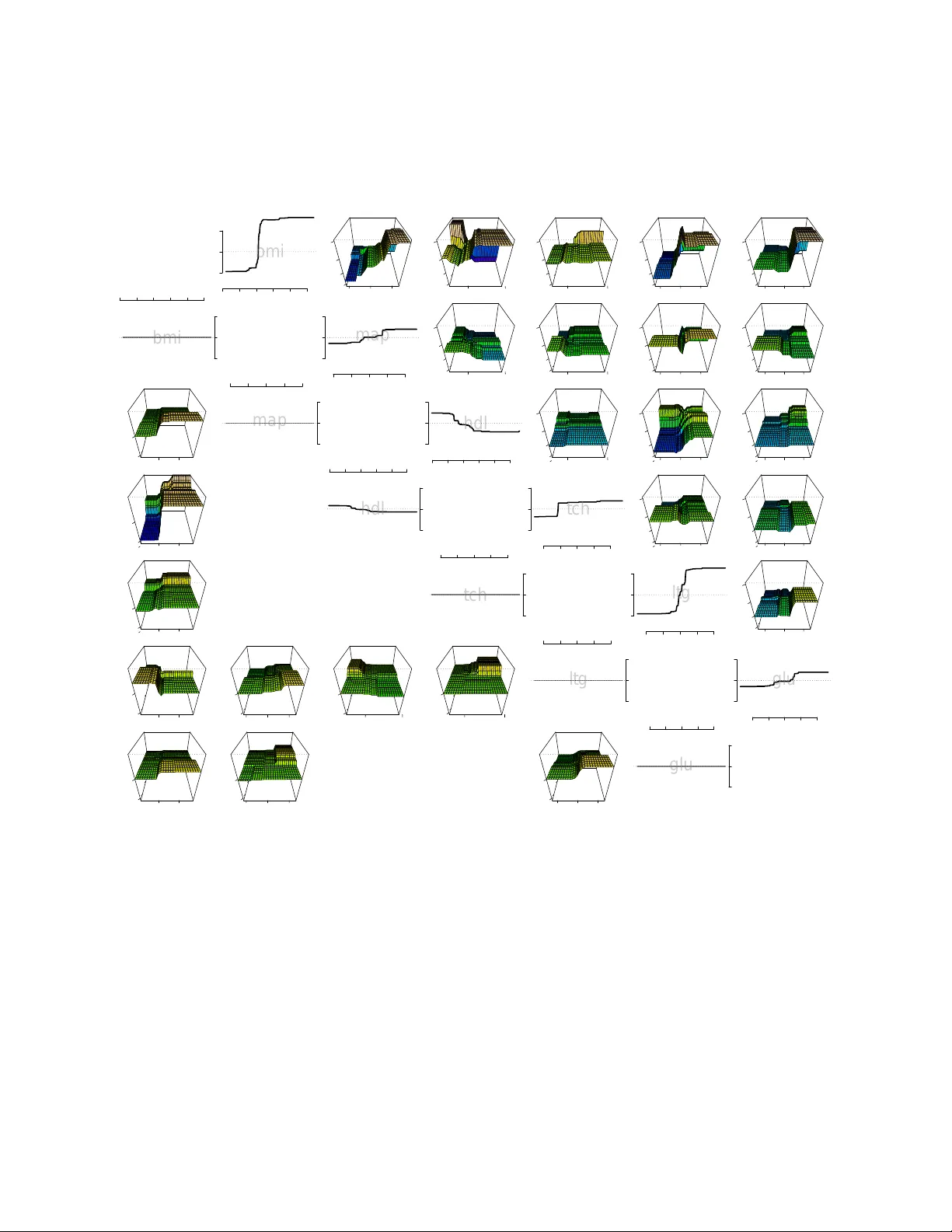
F orest Garrote Nicolai Meinshausen ∗ No v em b er 19, 2021 Abstract V ariable selection for high-dimensional linear mo dels has received a lot of attention lately , mostly in the con text of ` 1 -regularization. P art of the attraction is the v ari- able selection effect: parsimonious mo dels are obtained, whic h are very suitable for in terpretation. In terms of predictiv e p o wer, how ev er, these regularized linear mo dels are often slightly inferior to machine learning pro cedures like tree ensem bles. T ree ensem bles, on the other hand, lac k usually a formal w ay of v ariable selection and are difficult to visualize. A Garrote-style con vex p enalt y for trees ensembles, in particular Random F orests, is prop osed. The p enalt y selects functional groups of no des in the trees. These could b e as simple as monotone functions of individual predictor v ariables. This yields a parsimonious function fit, whic h lends itself easily to visualization and in terpretation. The predictive p ow er is main tained at least at the same level as the original tree ensemble. A key feature of the metho d is that, once a tree ensemble is fitted, no further tuning parameter needs to b e selected. The empirical performance is demonstrated on a wide array of datasets. 1 In tro duction Giv en data ( X i , Y i ), for i = 1 , . . . , n , with a p -dimensional real-v alued predictor v ariable X , where X = ( X (1) , . . . , X ( p ) ) ∈ X , and a real-v alued resp onse Y , a typical goal of regression analysis is to find an estimator ˆ Y ( x ), suc h that the exp ected loss E  L ( ˆ Y ( X ) , X )  is minimal, under a giv en loss function L : X × R 7→ R + . F or the following, the standard squared error loss is used. If the predictor can b e of the ‘black-box’ type, tree ensem bles hav e prov en to b e very p ow erful. Random F orests (Breiman, 2001) is a prime example, as are b oosted regression trees (Y u and B ¨ uhlmann, 2003). There are man y in teresting to ols a v ailable for in terpretation of these tree ensembles, see for example Strobl et al. (2007) and the references therein. ∗ Departmen t of Statistics, Univ ersity of Oxford, 1 South Parks Road, OX1 3TG, UK 1 While tree ensembles often hav e very go o d predictiv e p erformance, an adv an tage of a linear mo del is b etter in terpretabilit y . Measuring v ariable imp ortance and p erforming v ari- able selection are more easier to formulate and understand in the con text of linear mo dels. F or high-dimensional data with p  n , regularization is clearly imp erative and the Lasso (Tibshirani, 1996; Chen et al., 2001) has pro ven to b e very p opular in recen t y ears, since it com bines a con vex optimization problem with v ariable selection. A precursor to the Lasso w as the nonnegative Garrote (Breiman, 1995). A disadv an tage of the nonnegative Garrote is the reliance on an initial estimator, which could b e the least squares estimator or a regu- larized v ariation. On the p ositive side, imp ortant v ariables incur less p enalty and bias under the regularization than they do with the Lasso. F or a deeper discussion of the prop erties of the nonnegative Garrote see Y uan and Lin (2007). Here, it is prop osed to use Random F orest as an initial estimator for the nonnegative Garrote. The idea is related to the Rule Ensemble approac h of F riedman and P op escu (2008), who used the Lasso instead of the nonnegative Garrote. A crucial distinction is that rules fulfilling the same functional role are group ed in our approac h. This is similar in spirit to the group Lasso (Meier et al., 2008; Y uan and Lin, 2006; Zhao, Ro c ha, and Y u, Zhao et al.). This pro duces a very accurate predictor that uses just a few functional groups of rules, discarding many v ariables in the pro cess as irrelev an t. A unique feature of the proposed metho d is that is seems to w ork v ery well in the absence of a tuning parameter. It just requires the choice of an initial tree ensemble. This makes the pro cedure very simple to implement and computationally efficient. The idea and the algorithm is developed in Section 2, while a detailed n umerical study on 15 datasets mak es up Section 3. 2 Metho ds 2.1 T rees and Equiv alent Rules A tree T is seen here as a piecewise-constant function R p 7→ R derived from the tree structure in the sense of Breiman et al. (1984). F riedman and Popescu (2008) prop osed ‘rules’ as a name for simple rectangular-shap ed indicator functions. Every no de j in a tree is associated with a B j in R p -dimensional space, defined as the set of all v alues x ∈ R p that pass through no de j if passed down the tree. All v alues x ∈ R p that do not pass throuh no de j are outside of B j . The w a y rules are used here, they corresp ond to indicator functions R = R j , R j ( x ) =  1 X ∈ B j 0 X / ∈ B j , i.e. R j ( x ) = 1 { X ∈ B j } is the indicator function for b ox B j . F or a more detailed discussion see F riedman and Popescu (2008). 2 T o give an example of a rule, tak e the well-kno w dataset on abalone (Nash et al., 1994) as an example. The goal is to predict age of abalone from ph ysical measuremen ts. F or eac h of the 4177 abalone in the dataset, eigh t predictor v ariables (sex, length, diameter, height, while w eight, sh uc k ed weigh t, viscera w eigh t and shell w eigh t) are av ailable. An example of a rule is R 1 ( x ) = 1 { diameter ≥ 0 . 537 and shell weigh t ≥ 0 . 135 } , (1) and the presence of such a rule in a final predictor is easy to interpret, comparable to in terpreting co efficients in a linear mo del. F or the follo wing, it is assumed that rules con tain at most a single inequalit y for each v ariable. In other w ords, the b o xes defined by rules in p -dimensional spaces are defined by at most a single hyperplane in eac h v ariable. If a rule violates this assumption, it can easily b e decomp osed into tw o or sev eral rules satisfying the assumption. Ev ery regression tree can b e written as a linear superp osition of rules. Suppose a tree T has J no des in total. The regression function ˆ T of this tree (ensemble) can then b e written as ˆ T ( x ) = J X j =1 ˆ β tree j R j ( x ) (2) for some ˆ β tree . The decomp osition is not unique in general. W e could, for example, assign non-zero regression co efficien ts ˆ β j only to leaf no des. Here, we build the regression function incremen tally instead, assigning non-zero regression co efficients to al l no des. The v alue ˆ β tree j are defined as ˆ β tree j =  E n ( Y | Y ∈ B j ) − E n ( Y | Y ∈ B pa ( j ) ) if j is not ro ot no de E n ( Y ) if j is ro ot no de , (3) where E n is the empirical mean across the n observ ations and pa ( j ) is the paren t node of j in the tree. Rule (1), in the abalone example ab ov e, receiv es a regression weigh t ˆ β tree 1 = 0 . 0237. The contribution of rule (1) to the Random F orest fit is thus to increase the fitted v alue if and only if the diameter is larger than 0.537 and shell weigh t is larger than 0.135. The Random F orest fit is the sum of the contribution from all these rules, where eac h rule corresponds to one no de in the tree ensemble. T o see that (2) and (3) really correspond to the original tree (ensemble) solution, consider just a single tree for the momen t. Denote the predicted v alue for predictor v ariable X by ˆ T ( x ). Let B le af ( x ) b e the rectangular area in p -dimensional space that corresp onds to the leaf node le af ( x ) of the tree in which predictor v ariable X falls. The predicted v alue follo ws then by adding up all relev ant nodes and obtaining with (2) and (3), ˆ T ( x ) = E n ( Y | Y ∈ B le af ( x ) ) , i.e. the predicted v alues is just the empirical mean of Y across all observ ations i = 1 , . . . , n whic h fall in to the same leaf no de as X , whic h is equiv alent to the original prediction of the 3 tree. The equiv alence for tree ensem bles follows by av eraging across all individual trees as in (2). 2.2 Rule Ensem bles The idea of F riedman and P op escu (2008) is to mo dify the co efficients ˆ β tree in (2), increasing sparsit y of the fit b y setting many regression co efficient to 0 and eliminating the correspond- ing rules from the fit, while hop efully not degrading the predictive p erformance of the tree ensem ble in the pro cess. The rule ensem ble predictors are th us of the form J X j =1 ˆ β j R j ( x ) . (4) Sparsit y is enforced b y p enalizing the ` 1 -norm of ˆ β in LASSO-st yle (Tibshirani, 1996), ˆ β re ; λ = argmin β n X i =1 ( Y i − J X j =1 β j R j ( X i )) 2 suc h that J X j =1 | β j | ≤ λ. (5) This enforces sparsity in terms of rules, i.e. the final predictor will hav e typically only v ery few rules, at least compared to the original tree ensemble. The penalty parameter λ is t ypically c hosen by cross-v alidation. F riedman and P op escu (2008) recommend to add the linear main effects of all v ariables into (5), whic h w ere omitted here for notational simplicit y and to keep in v ariance with resp ect to monotone transformations of predictor v ariables. It is sho wn in F riedman and P op escu (2008) that the rule ensem ble estimator main tains in general the predictive abilit y of Random F orests, while lending itself more easily to interpretation. 2.3 F unctional grouping of rules The rule ensemble approach is treating all rules equally b y enforcing a ` 1 -p enalt y on all rules extracted from a tree ensem ble. It do es not take in to account, ho wev er, that there are t ypically many v ery closely related rules in the fit. T ake the RF fit to the abalone data as an example. Sev eral h undred rules are extracted from the RF, tw o of whic h are R 1 ( x ) = 1 { diameter ≥ 0 . 537 and shell weigh t ≥ 0 . 135 } , (6) with regression co efficient ˆ β 1 = 0 . 023 and R 2 ( x ) = 1 { diameter ≥ 0 . 537 and shell weigh t ≥ 0 . 177 } , (7) with regression coefficient ˆ β 2 = 0 . 019. The effect of these tw o rules, measured b y ˆ β 1 R 1 and ˆ β 2 R 2 , are clearly very similar. In total, there are 32 rules ‘interaction’ rules that in volv e 4 0.0 0.2 −0.1 0.0 0.1 −1 0 1 0.0 0.2 −0.1 0.0 0.1 −1 0 0.0 0.2 −0.1 0.0 0.1 0 1 0.0 0.2 −0.1 0.0 0.1 0 2 0.0 0.2 −0.1 0.0 0.1 −0.01 0.00 0.01 0.0 0.2 −0.1 0.0 0.1 −0.01 0.00 0.01 0.0 0.2 −0.1 0.0 0.1 −0.01 0.00 0.01 0.0 0.2 −0.1 0.0 0.1 0 10 0.0 0.2 −0.1 0.0 0.1 −0.01 0.00 0.01 0.0 0.2 −0.1 0.0 0.1 0 10 Figure 1: FIRST COLUMN: c ombine d variable inter action rules b etwe en pr e dictor variable tc h (x-axis to the right) and ltg (y-axis to the left) in the R andom F or est fit for the Diab etes data. SECOND COLUMN: the inter action rules c an b e de c omp ose d into the effe cts ˆ T σ (plot- te d on z-axis) of four inter action p atterns σ = (+ , − ) on top, (+ , +) on se c ond fr om top, ( − , +) on se c ond fr om b ottom and ( − , − ) on the b ottom. THIRD COLUMN: applying the Garr ote c orr e ction, thr e e of the four inter action p atterns ar e set to 0. FOUR TH COLUMN: adding the four inter action p atterns with Garr ote c orr e ction up, the total inter action p attern b etwe en the two variables ltg and tc h in the F or est Garr ote fit. 5 v ariables diameter and shell weigh t in the RF fit to the abalone data. Selecting some mem b ers of this group, it seems artificial to exclude others of the same ‘functional’ type. Sparsit y is measured purely on a rule-b y-rule basis in the ` 1 -p enalt y term of rule ensembles (5). Selecting the t w o rules men tioned ab ov e incurs the same sparsity p enalt y as if the second rule in volv ed tw o completely different v ariables. An undesirable side-effect of not taking into accoun t the grouping of rules is that man y or even all original predictor v ariables might still b e in volv ed in the rules; sparsity is not explicitly enforced in the sense that many irrelev ant original predictor v ariables are completely discarded in the selected rules. It seems natural to let rules form functional groups. The question then turns up which rules form useful and interpretable groups. There is clearly no simple righ t or wrong answ er to this question. Here, a very simple yet hop efully intuitiv e functional grouping of rules is emplo yed. F or the j -th rule, with co efficien t ˆ β j , define the in teraction pattern σ j = ( σ j, 1 , . . . , σ j,p ) for v ariables k = 1 , . . . , p b y σ j,k =      +1 iff sup x,x 0 ∈ R p : x ( k ) >x 0 ( k ) ˆ β j ( R j ( x ) − R j ( x 0 )) > 0 − 1 iff inf x,x 0 ∈ R p : x ( k ) >x 0 ( k ) ˆ β j ( R j ( x ) − R j ( x 0 )) < 0 0 otherwise . (8) The meaning of in teraction patterns is b est understo o d if lo oking at examples for v arying degrees, where the degree of a interaction pattern σ is understo o d to b e the n umber of non-zero en tries in σ and corresp onds to the n umber of v ariables that are in volv ed in a rule. First degree (main effects). The simplest in teraction patterns are those in volving a single v ariable only , which corresp ond in some sense to the main effects of v ariables. The in teraction pattern (0 , + , 0 , 0 , 0 , 0 , 0 , 0) for example collects all rules that inv olv e the 2nd predictor v ariable length only and lead to a monotonically increasing fit (are thus of the form 1 { length ≤ u } for some real-v alued u if the corresp onding regression co efficien t w ere p ositiv e or 1 { length ≥ u } if the regression co efficien t w ere negativ e). The in teraction pattern (0 , 0 , − , 0 , 0 , 0 , 0 , 0) collects con versely all those rules that yield a monotonically decreasing fit in the v ariable diameter , the third v ariable. Second degree (in teractions effects). Second degree in teraction patterns are of the form (6) or (7). As diameter is the 3rd v ariable and shell w eight the 8th, the in teraction pattern of b oth rules (6) and (7) is (0 , 0 , + , 0 , 0 , 0 , 0 , +) , making them members of the same functional group, as for b oth rules the fitted v alue is monotonically increasing in b oth inv olved v ariables. In other w ords, either a large v alue in 6 b oth v ariables increases the fitted v alue or a very low v alue in b oth v ariables decreases the fitted v alue. Second degree interaction patterns thus form four categories for eac h pair of v ariables. A case could b e made to merge these four categories into just tw o categories, as the interaction patterns do not conform nicely with the more standard multiplicativ e form of in teractions in linear mo dels. Ho wev er, there is no reason to b elieve that nature alwa ys adheres to the m ultiplicative form of in teractions typically assumed in linear mo dels. The in teraction patterns used here seemed more adapted to the context of rule-based inference. F actorial v ariables can b e dealt with in the same framework (8) b y conv erting to dumm y v ariables first. 2.4 Garrote correction and selection In contrast to the group Lasso approach of Y uan and Lin (2006), the prop osed metho d do es not only start with knowledge of natural groups of v ariables or rules. A very go o d initial estimator is av ailable, namely the Random F orest fit. This is exploited in the following. Let ˆ T σ b e the part of the fit that collects all contributions from rules with interaction pattern σ , ˆ T σ ( x ) = X j : σ ( ˆ β j R j )= σ ˆ β j R j ( x ) . (9) Let G b e the collection of all p ossible interaction patterns σ . The tree ensemble fit (2) can then b e re-written as a sum ov er all interaction patterns ˆ T ( x ) = X σ ∈G ˆ T σ ( x ) . (10) A interaction pattern σ is called active if the corresp onding fit in the tree ensem ble is non- zero, i.e. if and only if ˆ T σ is not identically 0. The Random F orest fit con tains very often a h uge n umber of active in teraction pattern, inv olving in teractions up to fourth and higher degrees. Most of those activ e patterns con tribute just in a negligible w a y to the ov erall fit. The idea prop osed here is to use (10) as a starting p oint and modify it to enforce sparsity in the final fit, getting rid of as many unnecessary predictor v ariables and asso ciated in ter- action patterns as p ossible. The Lasso of Tibshirani (1996) w as used in the rule ensem ble approac h of F riedman and Popescu (2008). Here, ho w ever, the starting p oint is the func- tional decomp osition (10), whic h is already a very go od initial (y et not sparse) estimator of the underlying regression function. Hence it seems more appropriate to use Breiman’s nonnegative Garrote (Breiman, 1995), p enalizing con tributions of in teraction patterns less if their con tribution to the initial es- timator is large and vice versa. The b eneficial effect of this bias reduction for imp ortan t v ariables has b een noted in, amongst others, Y uan and Lin (2007) and Zou (2006). 7 The Garrote-style F orest estimator ˆ T g ar is defined as ˆ T g ar = X σ ∈G γ σ ˆ T σ . (11) Eac h contribution ˆ T σ of an in teraction pattern σ is multiplied by a factor ˆ γ σ . The original tree ensemble fit is obtained by setting all factors equal to 1. The m ultiplicative factor γ is chosen b y least squares, sub ject to the constrain t that the total ` 1 -norm of the m ultiplying co efficients is less than 1, ˆ γ = argmin γ n X i =1 ( Y i − X σ ∈G γ σ ˆ T σ ( X i )) 2 suc h that |G | − 1 X σ ∈G | γ σ | ≤ 1 and min σ ∈G γ σ ≥ 0 . (12) The normalizing factor |G | − 1 divides the ` 1 -norm of γ b y the total n um b er of in teraction patterns and is certainly not crucial here but simplifies notation. The estimation of ˆ γ is an application of Breiman’s nonnegative Garrote (Breiman, 1995). As for the Garrote, the original predictors ˆ T σ are not rescaled, thus putting effectiv ely more p enalty on unimp ortan t predictors, with little v ariance of ˆ T σ across the samples X 1 , . . . , X n and less p enalt y on the imp ortan t predictors with higher v ariance, see (Y uan and Lin, 2007) for details. Algorithmically , the problem can b e solved with an efficien t Lars algorithm (Efron et al., 2004), whic h can easily b e adapted to include the p ositivit y constrain t. Alternativ ely , quadratic programming can b e used. It migh t b e surprising to see the ` 1 -norm constrained b y 1 instead of a tuning parameter λ . Y et this is indeed one of the in teresting prop erties of F orest Garrote. The tree ensemble is in some sense selecting a goo d lev el of sparsit y . It seems maybe implausible that this w ould w ork in practice, but some intuitiv e reasons for its empirical success are giv en further b elow and ample empirical evidence is provided in the section with n umerical results. A dra wback of the Garrote in the linear mo del setting is the reliance on the OLS estimator (or another suitable estimator), see also Y uan and Lin (2007). The OLS estimator is for example not a v ailable if p > n . The tree ensemble estimates are, in contrast, v ery reasonable estimators in a wide v ariety of settings, certainly including the high-dimensional setting p  n . The entire F orest Garrote algorithm w orks thus as follo ws 1. Fit Random F orest or another tree ensem ble approach to the data. 2. Extract ˆ T σ from the tree ensem ble for all σ ∈ G by first extracting all rules R j and corresp onding regression co efficien ts ˆ β j and grouping them via (9) for each interaction pattern. 8 3. Estimate ˆ γ as in (12) from the data, using for example the LARS algorithm (Efron et al., 2004). 4. The fitted F orest Garrote function ˆ T g ar is given b y (11). The whole algorithm is very simple and fast, as there is no tuning parameter to choose. 2.5 Lac k of tuning parameter In most regularization problems, lik e the Lasso (Tibshirani, 1996), choosing the regulariza- tion parameter is very imp ortan t and it is usually a priori not clear what a go o d choice will b e, unless the noise lev el is kno wn with go o d accuracy (and it usually it is not). The most ob vious approach would b e cross-v alidation. Cross-v alidation can b e computationally exp ensiv e and is usually not guaranteed to lead to optimal sparsity of the solution, select- ing many more v ariables or interaction patterns than necessary , as shown for the Lasso in Meinshausen and B ¨ uhlmann (2006) and Leng et al. (2006). Since the starting point is a very useful predictor, the original tree ensemble, there is a natural tuning parameter for the F orest Garrote estimator. As noted b efore, γ = (1 , 1 , 1 , . . . , 1 , 1) corresp onds to the original tree ensemble solution. The original tree ensem- ble solution ˆ T is thus con tained in the feasible region of the optimization problem (12) under a constrain t on the ` 1 -norm of exactly 1. The solution (11) will thus b e at least as sparse as the original tree ensemble solution in the sense if sparsity is measured in the same ` 1 -norm sense as in (12). Some v ariables migh t not b e used at all even though they app ear in the original tree ensemble. On the other hand, the empirical squared error loss of ˆ T g ar is at least as lo w (and t ypically lo w er) than for the original tree ensemble solution as ˆ γ will reduce the empirical loss among all solutions in the feasible region of (12), whic h contains the original tree ensemble solution. The latter p oint do es clearly not guaran tee b etter generalization on yet unseen data, but a constrain t of 1 on the ` 1 -norm turns out to b e an in teresting starting p oint and is a very go o d default choice of the p enalt y parameter. Sometimes one migh t still b e in terested in introducing a tuning parameter. One could replace the constraint of 1 on the ` 1 -norm of γ in (12) b y a constraint λ , ˆ γ = argmin γ n X i =1 ( Y i − X σ ∈G γ σ ˆ T σ ( X i )) 2 suc h that |G | − 1 X σ ∈G | γ σ | ≤ λ and min σ ∈G γ σ ≥ 0 . (13) The range o ver whic h to searc h, with cross-v alidation, to ov er λ can then typically be limited to [0 , 2]. Empirically , it turned out that the default choice λ = 1 is very reasonable and actually achi eves often b etter predictiv e and selection p erformance than the cross-v alidated solution, since the latter suffers from p ossibly high v ariance for finite sample sizes. 9 −0.10 0.00 0.10 bmi −10 0 10 0. 0 0. 1 −0.1 0.0 0.1 −2 0 2 4 0.0 0.1 0.0 0.2 −2 0 2 4 0.0 0.1 0.0 0.2 −2 0 2 4 0. 0 0 .1 −0.1 0.0 0.1 −2 0 2 4 0.0 0.1 −0.1 0.0 0.1 −2 0 2 4 − 0.10 0.00 0.10 −10 0 10 bmi −0.10 0.00 0.10 map −10 0 10 − 0.1 0.0 0.1 0.0 0.2 −2 0 2 4 −0.1 0.0 0.1 0.0 0.2 −2 0 2 4 −0.1 0.0 0.1 −0.1 0.0 0.1 −2 0 2 4 −0.1 0.0 0.1 −0.1 0.0 0.1 −2 0 2 4 −0.1 0.0 0.1 0.0 0.1 −50 0 −0.10 0.00 0.10 −10 0 10 map −0.10 0.00 0.10 hdl −10 0 10 0 .0 0.2 0.0 0.2 −2 0 2 4 0. 0 0.2 −0.1 0.0 0.1 −2 0 2 4 0 .0 0.2 −0.1 0.0 0.1 −2 0 2 4 0. 0 0.2 0.0 0.1 −50 0 1:10 1:10 −0.10 0.00 0.10 −10 0 10 hdl −0.05 0.05 0.15 tch −10 0 10 0.0 0.2 −0.1 0.0 0.1 −2 0 2 4 0 .0 0.2 −0.1 0.0 0.1 −2 0 2 4 0.0 0.2 0.0 0.1 −50 0 1:10 1:10 1:10 1:10 −0.05 0.05 0.15 −10 0 10 tch −0.10 0.00 0.10 ltg −10 0 10 − 0.1 0 .0 0.1 −0.1 0.0 0.1 −2 0 2 4 −0.1 0.0 0.1 0.0 0.1 −50 0 −0.1 0.0 0.1 −0.1 0.0 0.1 −50 0 −0.1 0.0 0.1 0.0 0.2 −50 0 −0.1 0.0 0.1 0.0 0.2 −50 0 −0.10 0.00 0.10 −10 0 10 ltg −0.10 0.00 0.10 glu −10 0 10 −0.1 0.0 0.1 0.0 0.1 −50 0 −0.1 0.0 0.1 −0.1 0.0 0.1 −50 0 1:10 1:10 −0.1 0.0 0.1 −0.1 0.0 0.1 −50 0 −0.10 0.00 0.10 −10 0 10 glu Figure 2: UPPER RIGHT DIAGONAL: ‘main effe cts’ and ‘inter actions’ of se c ond de gr e e for the R andom F or est fit on the Diab etes data b etwe en the main 6 variables (not showing al l variables). LO WER LEFT DIA GONAL: c orr esp onding functions for the F or est Garr ote. Some main effe cts and inter actions ar e set exactly to zer o. V anishing inter actions ar e not plotte d, le aving some entries blank. 10 2.6 Example: diab etes data The metho d is illustrated on the diabetes data from Efron et al. (2004) with p = 10 pre- dictor v ariables, age, sex, b o dy mass index, a verage blo o d pressure and six blo o d serum measuremen ts. These v ariables were obtained for eac h of n = 442 diab etes patients, along with the resp onse of interest, a ‘quantitativ e measure of disease progression one year after baseline’. Applying a Random F orest fit to this dataset, the main effects and second-order in teractions effects, extracted as in (9), are sho wn in the upper right diagonal of Figure 2, for 6 out of the 10 v ariables (c hosen at random to facilitate presentation). All of these v ariables ha v e non-v anishing main effects (on the diagonal) and the interaction patterns can b e quite complex, making them somewhat difficult to in terpret. No w applying a F orest Garrote selection to the Random F orest fit, one obtains the main effects and in teraction plots sho wn in the lo wer left diagonal of Figure 2. Note that the x-axis in the in teraction plots corresponds to the v ariable in the same column, while the y-axis refers to the v ariable in the same row. Interaction plots are th us rotated by 90 degrees b et w een the upper right and the lo wer left diagonal. Some main effects and in teractions are set to 0 b y the F orest Garrote selection. In teraction effects that are not set to 0 are t ypically ‘simplified’ considerably . The same effect was observ ed and explained in Figure 1. The interaction plot of F orest Garrote seems thus m uc h more amenable for interpretation. 3 Numerical Results T o examine the predictive accuracy , v ariable selection prop erties and computational sp eed, v arious standard datasets are used and augmented with tw o higher-dimensional datasets. The first of these is a motif regression dataset (henceforth called ‘motif ’, p = 660 and n = 2587). The goal of the data collection is to help find transcription factor binding sites (motifs) in DNA sequences. The real-v alued predictor v ariables are abundance scores for p candidate motifs (for each of the genes). Our dataset is from a heat-sho c k exp eriment with y east. F or a general description and motiv ation about motif regression see Conlon et al. (2003). The metho d is applied to a gene expression dataset (‘vitamin’) whic h is kindly pro vided b y DSM Nutritional Pro ducts (Switzerland). F or n = 115 samples, there is a contin uous resp onse v ariable measuring the logarithm of rib oflavin (vitamin B2) pro duction rate of Bacillus Subtilis, and there are p = 4088 con tinuous cov ariates measuring the logarithm of gene expressions from essentially the whole genome of Bacillus Subtilis. Certain mutations of genes are thought to lead to higher vitamin concentrations and the challenge is to identify those relev ant genes via regression, p ossibly using also interaction betw een genes. In addition, the diab etes data from Efron et al. (2004) (‘diab etes’, p = 10 , n = 442), men tioned already ab ov e, are considered, the LA Ozone data (‘ozone’, p = 9 , n = 330), 11 ● ● ● ● ● ● ● ● ● ● ● ● ● ● ● 0.0 0.2 0.4 0.6 0.8 0.0 0.2 0.4 0.6 0.8 RANDOM FOREST FOREST GARROTE motifs ozone marketing bones galaxy boston prostate vitamin diabetes friedman abalone mpg auto machine concrete UNEXPLAINED VARIANCE ● ● ● ● ● ● ● ● ● ● ● ● ● ● ● 0.0 0.2 0.4 0.6 0.8 0.0 0.2 0.4 0.6 0.8 RANDOM FOREST FOREST GARROTE (CV) motifs ozone marketing bones galaxy boston prostate vitamin diabetes friedman abalone mpg auto machine concrete UNEXPLAINED VARIANCE ● ● ● ● ● ● ● ● ● ● ● ● ● ● ● 0.0 0.2 0.4 0.6 0.8 0.0 0.2 0.4 0.6 0.8 RANDOM FOREST RULE ENSEMBLES motifs ozone marketing bones galaxy boston prostate vitamin diabetes friedman abalone mpg auto machine concrete Figure 3: The unexplaine d varianc e on test data, as a fr action of the total varianc e. LEFT: Comp arison of unexplaine d varianc e for F or est Garr ote versus R andom F or ests. MIDDLE: F or est Garr ote (CV) versus R andom F or ests. RIGHT: R ule Ensembles versus R andom F or ests. and also the dataset about marketing (‘marketing’, p = 14 , n = 8993), b one mineral densit y (‘b one’, p = 4 , n = 485), radial v elo cit y of galaxies (‘galaxies’, p = 4 , n = 323) and prostate cancer analysis (‘prostate’, p = 9 , n = 97); the latter all from Hastie et al. (2001). The chosen resp onse v ariable is ob vious in each dataset. See the v ery worth while b ook Hastie et al. (2001) for more details. T o giv e comparison on more widely used datasets, F orest Garrote is applied to v arious dataset from the UCI mac hine learning rep ository (Asuncion and Newman, 2007), ab out predicting fuel efficiency (‘auto-mpg’, p = 8 , n = 398), compressive strength of concrete (‘concrete’, p = 9 , n = 1030), median house prices in the Boston area (‘housing’ , p = 13 , n = 506), CPU p erformance (‘mac hine’, p = 10 , n = 209) and finally the first of three artificial datasets in F riedman (1991). The unexplained v ariance on test data for all these datasets with F orest Garrote is com- pared with that of Random F orests and Rule Ensembles in Figure 3. The tuning parameters in Random F orests (namely ov er ho w man y randomly selected v ariables to search for the b est splitp oint) is optimized for eac h dataset, using the out-of-bag p erformance measure. F or comparison b etw een the metho ds, the data are split into tw o parts of equal size, one half for training and the other for testing. Results are compared with F orest Garrote (CV), where the tuning parameter λ in (13) is not chosen to b e 1 as for the standard F orest Garrote es- timator, but is instead chosen by cross-v alidation. There are tw o main conclusions from the Figure. First, all three metho d (F orest Garrote, F orest Garrote (CV) and Rule Ensem bles) 12 dataset n p F orest Garrote F orest Garrote (CV) Rule Ensembles motifs 1294 666 88.5 425 933 ozone 165 9 0.26 2.7 16.5 mark eting 3438 13 6.09 32.5 696 b ones 242 3 0.05 1.1 26.2 galaxy 162 4 0.07 1.1 40.2 b oston 253 13 0.79 5.3 87.5 prostate 48 8 0.25 3.3 2.4 vitamin 58 4088 1.98 21.6 39 diab etes 221 10 0.64 4.8 31.2 friedman 150 4 0.1 1.3 16.6 abalone 2088 8 0.59 5.1 808 mpg 196 7 0.18 1.9 36.6 auto 80 24 2.99 22 154 mac hine 104 7 0.29 2.5 19.6 concrete 515 8 0.58 4.3 271 T able 1: The r elative CPU time sp ent on F or est Garr ote, F or est Garr ote (CV) and Rule Ensembles for the various datasets. F or est Garr ote uses the le ast c omputational r esour c es sinc e (i) it starts fr om a r elative smal l set of dictionary elements (al l ˆ T σ for σ ∈ G as opp ose d to al l rules), (ii) the solution has to b e c ompute d only for a single r e gularization p ar ameter and ther e is henc e (iii) also no ne e d for exp ensive cr oss-validation. Note that the times ab ove ar e only for the rule sele ction steps (5) and (12) r esp e ctively and the over al l r elative sp e e d differ enc e is typic al ly smal ler as a tr e e ensemble fit ne e ds to b e c ompute d as an initial estimator in al l settings. outp erformed Random F orests in terms of predictive accuracy on almost all datasets. Sec- ond, the relativ e difference b et ween these three metho ds is v ery small. Maybe surprisingly , using a cross-v alidated c hoice of λ did not help muc h in improving predictiv e accuracy for the F orest Garrote estimator. On the contrary , it rather lead to w orse predictive p erformance, presumably due to the inherent v ariability of the selected p enalty parameter. F orest Garrote (CV) has also ob viously a computational disadv antage compared with the recommended F orest Garrote estimator, as sho wn in T able 1 which is comparing relativ e CPU times necessary to compute the relative estimators. All three metho ds could be speeded up considerably b y clever computational implemen tation. An y suc h improv ement w ould most lik ely b e applicable to any of these three compared metho ds as they hav e very similar optimization problems at their heart. Only relative p erformance measurements seem to b e appropriate and only the time it takes to solve the resp ectiv e optimization problems (5), (12) and (13) is rep orted, including time necessary for cross-v alidation, if so required. Rule 13 dataset n p F orest Garrote Rule Ensem bles Random F orests motifs 1294 666 44 75 233 ozone 165 9 8 8 9 mark eting 3438 13 9 13 13 b ones 242 3 3 3 3 galaxy 162 4 4 4 4 b oston 253 13 9 13 13 prostate 48 8 8 8 8 vitamin 58 4088 45 67 648 diab etes 221 10 7 8 10 friedman 150 4 4 4 4 abalone 2088 8 5 7 8 mpg 196 7 7 7 7 auto 80 24 16 15 21 mac hine 104 7 7 7 7 concrete 515 8 8 8 8 T able 2: The numb er of variables sele cte d in total for F or est Garr ote, Rule Ensembles and R andom F or ests. F or est Garr ote and R ule Ensembles prune the numb er of variables use d c onsider ably, esp e cial ly for higher-dimensional data. Ensem bles is faring b y far the worst here, since the underlying optimization problem is v ery high-dimensional. The dimensionality J in (5) is the total n um b er of rules, which corresp onds to the n umber of all no des in the Random F orest fit. The total num b er |G | of in teraction patterns in the optimization underlying (12) in the F orest Garrote fit is, on the other hand, v ery muc h smaller than the num b er J of all rules, since many rules are t ypically combined in each in teraction patterns. The lack of cross-v alidation for the F orest Garrote estimator clearly also sp eeds computation up b y an additional factor b etw een 5 and 10, dep ending on whic h form of cross-v alidation is employ ed. Finally , the num b er of v ariables selected b y either metho d is examined. A v ariable is said to b e selected for this purp ose if it app ears in any no de in the F orest or in an y rule that is selected with a non-zero co efficien t. In other w ords, selected v ariables will b e needed to compute predictions, not selected v ariables can b e discarded. The results are sho wn in T able 2. Man y v ariables are t ypically inv olved in a Random F orest Fit and b oth Rule Ensem bles as well as F orest Garrote can cut do wn this n um b er substan tially . Esp ecially for higher-dimensional data with large n umber p of v ariables, the effect can b e pronounced. Bet w een Rule Ensem bles and F orest Garrote, the differences are v ery minor with a slight tendency of F orest Garrote to pro duce sparser results. 14 4 Conclusions Balancing in terpretabilit y and predictiv e p o w er for regression problems is a difficult act. Linear mo dels lend themselv es more easily to interpretation but suffer often in terms of predictiv e p ow er. Random F orests (RF), on the other hand, are kno wn deliver v ery accurate prediction. T o ols exist to extract marginal v ariable imp ortance measures from RF. Ho wev er, the in terpretability of RF could b e improv ed if the v ery large num b er of no des in the h undreds of trees fitted for RF could b e reduced. Here, the F orest Garrote w as proposed as suc h a pruning metho d for RF or tree ensem bles in general. It collects all rules or no des in the F orest that b elong to the same functional group. Using a Garrote-st yle p enalty , some of these functional groups are then shrunken to zero, while the signal of other functional groups is enhanced. This leads to a sparser mo del and rather interpretable in teraction plots b etw een v ariables. Predictive p o w er is similar or b etter to the original RF fit for all examined datasets. The unique feature of F orest Garrote is that it seems to work very w ell without the use of a tuning parameter, as sho wn on m ultiple well kno wn and less well kno wn datasets. The lac k of a tuning parameter mak es the metho d v ery easy to implemen t and computationally efficien t. References Asuncion, A. and D. Newman (2007). UCI mac hine learning rep ository . Breiman, L. (1995). Better subset regression using the nonnegative garrote. T e chnomet- rics 37 , 373–384. Breiman, L. (2001). Random F orests. Machine L e arning 45 , 5–32. Breiman, L., J. F riedman, R. Olshen, and C. Stone (1984). Classific ation and R e gr ession T r e es . W adsw orth, Belmont. Chen, S., S. Donoho, and M. Saunders (2001). Atomic decomp osition by basis pursuit. SIAM R eview 43 , 129–159. Conlon, E., X. Liu, J. Lieb, and J. Liu (2003). Integrating regulatory motif discov ery and genome-wide expression analysis. Pr o c e e dings of the National A c ademy of Scienc e 100 , 3339 – 3344. Efron, B., T. Hastie, I. Johnstone, and R. Tibshirani (2004). Least angle regression. Annals of Statistics 32 , 407–451. F riedman, J. (1991). Multiv ariate adaptiv e regression splines. Annals of Statistics 19 , 1–67. 15 F riedman, J. and B. P op escu (2008). Predictiv e learning via rule ensem bles. Annals of Applie d Statistics , 916–954. Hastie, T., R. Tibshirani, J. F riedman, T. Hastie, J. F riedman, and R. Tibshirani (2001). The elements of statistic al le arning . Springer New Y ork. Leng, C., Y. Lin, and G. W ahba (2006). A note on the lasso and related pro cedures in mo del selection. Statistic a Sinic a 16 , 1273–1284. Meier, L., S. v an de Geer, and P . Buhlmann (2008). The group lasso for logistic regression. Journal of the R oyal Statistic al So ciety, Series B 70 , 53–71. Meinshausen, N. and P . B ¨ uhlmann (2006). High dimensional graphs and v ariable selection with the lasso. A nnals of Statistics 34 , 1436–1462. Nash, W., T. Sellers, S. T alb ot, A. Cawthorn, and W. F ord (1994). The population biology of abalone in tasmania. T ec hnical rep ort, Sea Fisheries Division. Strobl, C., A. Boulesteix, A. Zeileis, and T. Hothorn (2007). Bias in random forest v ariable imp ortance measures: Illustrations, sources and a solution. BMC Bioinformatics 8 , 25. Tibshirani, R. (1996). Regression shrink age and selection via the lasso. Journal of the R oyal Statistic al So ciety, Series B 58 , 267–288. Y u, B. and P . B ¨ uhlmann (2003). Bo osting with the L 2 loss: Regression and classification. Journal of the A meric an Statistic al Asso ciation 98 , 324–339. Y uan, M. and Y. Lin (2006). Mo del selection and estimation in regression with group ed v ariables. Journal of the R oyal Statistic al So ciety, Series B 68 , 49–67. Y uan, M. and Y. Lin (2007). On the nonnegative garrote estimator. Journal of the R oyal Statistic al So ciety, Series B 69 , 143–161. Zhao, P ., G. Ro cha, and B. Y u. The comp osite absolute p enalties family for group ed and hierarc hical v ariable selection. A nnals of Statistics, to app e ar . Zou, H. (2006). The adaptive lasso and its oracle prop erties. Journal of the Americ an Statistic al Asso ciation 101 , 1418–1429. 16